%20--%3e%3c!DOCTYPE%20svg%20PUBLIC%20'-//W3C//DTD%20SVG%201.0//EN'%20'http://www.w3.org/TR/2001/REC-SVG-20010904/DTD/svg10.dtd'%3e%3csvg%20version='1.0'%20id='Layer_1'%20xmlns='http://www.w3.org/2000/svg'%20xmlns:xlink='http://www.w3.org/1999/xlink'%20x='0px'%20y='0px'%20width='64px'%20height='64px'%20viewBox='5.5%20-3.5%2064%2064'%20enable-background='new%205.5%20-3.5%2064%2064'%20xml:space='preserve'%3e%3cg%3e%3ccircle%20fill='%23FFFFFF'%20fill-opacity='0'%20cx='37.785'%20cy='28.501'%20r='28.836'/%3e%3cpath%20fill='%23595959'%20d='M37.441-3.5c8.951,0,16.572,3.125,22.857,9.372c3.008,3.009,5.295,6.448,6.857,10.314%20c1.561,3.867,2.344,7.971,2.344,12.314c0,4.381-0.773,8.486-2.314,12.313c-1.543,3.828-3.82,7.21-6.828,10.143%20c-3.123,3.085-6.666,5.448-10.629,7.086c-3.961,1.638-8.057,2.457-12.285,2.457s-8.276-0.808-12.143-2.429%20c-3.866-1.618-7.333-3.961-10.4-7.027c-3.067-3.066-5.4-6.524-7-10.372S5.5,32.767,5.5,28.5c0-4.229,0.809-8.295,2.428-12.2%20c1.619-3.905,3.972-7.4,7.057-10.486C21.08-0.394,28.565-3.5,37.441-3.5z%20M37.557,2.272c-7.314,0-13.467,2.553-18.458,7.657%20c-2.515,2.553-4.448,5.419-5.8,8.6c-1.354,3.181-2.029,6.505-2.029,9.972c0,3.429,0.675,6.734,2.029,9.913%20c1.353,3.183,3.285,6.021,5.8,8.516c2.514,2.496,5.351,4.399,8.515,5.715c3.161,1.314,6.476,1.971,9.943,1.971%20c3.428,0,6.75-0.665,9.973-1.999c3.219-1.335,6.121-3.257,8.713-5.771c4.99-4.876,7.484-10.99,7.484-18.344%20c0-3.543-0.648-6.895-1.943-10.057c-1.293-3.162-3.18-5.98-5.654-8.458C50.984,4.844,44.795,2.272,37.557,2.272z%20M37.156,23.187%20l-4.287,2.229c-0.458-0.951-1.019-1.619-1.685-2c-0.667-0.38-1.286-0.571-1.858-0.571c-2.856,0-4.286,1.885-4.286,5.657%20c0,1.714,0.362,3.084,1.085,4.113c0.724,1.029,1.791,1.544,3.201,1.544c1.867,0,3.181-0.915,3.944-2.743l3.942,2%20c-0.838,1.563-2,2.791-3.486,3.686c-1.484,0.896-3.123,1.343-4.914,1.343c-2.857,0-5.163-0.875-6.915-2.629%20c-1.752-1.752-2.628-4.19-2.628-7.313c0-3.048,0.886-5.466,2.657-7.257c1.771-1.79,4.009-2.686,6.715-2.686%20C32.604,18.558,35.441,20.101,37.156,23.187z%20M55.613,23.187l-4.229,2.229c-0.457-0.951-1.02-1.619-1.686-2%20c-0.668-0.38-1.307-0.571-1.914-0.571c-2.857,0-4.287,1.885-4.287,5.657c0,1.714,0.363,3.084,1.086,4.113%20c0.723,1.029,1.789,1.544,3.201,1.544c1.865,0,3.18-0.915,3.941-2.743l4,2c-0.875,1.563-2.057,2.791-3.541,3.686%20c-1.486,0.896-3.105,1.343-4.857,1.343c-2.896,0-5.209-0.875-6.941-2.629c-1.736-1.752-2.602-4.19-2.602-7.313%20c0-3.048,0.885-5.466,2.658-7.257c1.77-1.79,4.008-2.686,6.713-2.686C51.117,18.558,53.938,20.101,55.613,23.187z'/%3e%3c/g%3e%3c/svg%3e)
%20--%3e%3c!DOCTYPE%20svg%20PUBLIC%20'-//W3C//DTD%20SVG%201.0//EN'%20'http://www.w3.org/TR/2001/REC-SVG-20010904/DTD/svg10.dtd'%3e%3csvg%20version='1.0'%20id='Layer_1'%20xmlns='http://www.w3.org/2000/svg'%20xmlns:xlink='http://www.w3.org/1999/xlink'%20x='0px'%20y='0px'%20width='64px'%20height='64px'%20viewBox='5.5%20-3.5%2064%2064'%20enable-background='new%205.5%20-3.5%2064%2064'%20xml:space='preserve'%3e%3cg%3e%3ccircle%20fill='%23FFFFFF'%20fill-opacity='0'%20cx='37.637'%20cy='28.806'%20r='28.276'/%3e%3cg%3e%3cpath%20fill='%23595959'%20d='M37.443-3.5c8.988,0,16.57,3.085,22.742,9.257C66.393,11.967,69.5,19.548,69.5,28.5c0,8.991-3.049,16.476-9.145,22.456%20C53.879,57.319,46.242,60.5,37.443,60.5c-8.649,0-16.153-3.144-22.514-9.43C8.644,44.784,5.5,37.262,5.5,28.5%20c0-8.761,3.144-16.342,9.429-22.742C21.101-0.415,28.604-3.5,37.443-3.5z%20M37.557,2.272c-7.276,0-13.428,2.553-18.457,7.657%20c-5.22,5.334-7.829,11.525-7.829,18.572c0,7.086,2.59,13.22,7.77,18.398c5.181,5.182,11.352,7.771,18.514,7.771%20c7.123,0,13.334-2.607,18.629-7.828c5.029-4.838,7.543-10.952,7.543-18.343c0-7.276-2.553-13.465-7.656-18.571%20C50.967,4.824,44.795,2.272,37.557,2.272z%20M46.129,20.557v13.085h-3.656v15.542h-9.944V33.643h-3.656V20.557%20c0-0.572,0.2-1.057,0.599-1.457c0.401-0.399,0.887-0.6,1.457-0.6h13.144c0.533,0,1.01,0.2,1.428,0.6%20C45.918,19.5,46.129,19.986,46.129,20.557z%20M33.042,12.329c0-3.008,1.485-4.514,4.458-4.514s4.457,1.504,4.457,4.514%20c0,2.971-1.486,4.457-4.457,4.457S33.042,15.3,33.042,12.329z'/%3e%3c/g%3e%3c/g%3e%3c/svg%3e)
1 Introduction
Laminar–turbulent transition of boundary-layer flows can have a strong impact on the performance of hypersonic vehicles because of its influence on the surface skin friction and aerodynamic heating. Therefore, the prediction and control of transition onset and the associated variation in aerothermodynamic parameters in high-speed flows is a key issue for optimizing the performance of the next-generation aerospace vehicles. Although many practical aerospace vehicles have blunt, hemispherical and ogival nose tips, the mechanisms that lead to boundary-layer instability and transition on such geometries are not fully understood as yet. A detailed review of boundary-layer transition over sharp and blunt cones in a hypersonic free stream is given by Schneider (Reference Schneider2004). As described therein, both experimental and numerical studies have shown that the modal growth of Mack-mode instabilities (or, equivalently, the so-called second-mode waves) is responsible for laminar–turbulent transition on sharp, axisymmetric cones at zero degrees angle of attack. Studies have also shown that increased nose-tip bluntness, e.g. a larger radius of the hemispherical or ogival nose tip, leads to the formation of an entropy layer that can extend well beyond the nose-tip region (Stetson Reference Stetson1983). This entropy layer has been shown to have a stabilizing effect on the amplification of Mack-mode instabilities, which is consistent with the observation that the onset of transition is displaced downstream as the nose bluntness is increased gradually from a sharp cone. However, while the boundary-layer flow continues to become more stable with increasing nose bluntness, experiments indicate that the downstream movement in transition slows down and eventually reverses when the nose bluntness exceeds a critical range (Stetson Reference Stetson1983).
A recent collaborative effort under the NATO STO group AVT-240 on Hypersonic Boundary-Layer Transition Prediction focused on the problem of transition on axisymmetric cones with blunt, hemispherical nose tips and on the potential role of transient growth in the transition reversal phenomenon (Paredes et al. Reference Paredes, Choudhari, Li, Jewell, Kimmel, Marineau and Grossir2019d). The collection of wind tunnel measurements from both U.S. and European facilities at free-stream Mach numbers from 6 to 10 confirmed the two distinct regions that are respectively referred to herein as the ‘small bluntness’ regime, wherein transition occurs well downstream of the nose tip, i.e. within the cone frustum, and progressively moves downstream with an increased bluntness, and the ‘large bluntness’ regime, where the transition location rapidly moves upstream as the nose bluntness in increased further. Transition onset within this ‘large bluntness’ regime was found to depend on uncontrolled disturbances due to nose-tip roughness. Beyond the critical nose Reynolds number for transition reversal at large bluntness values, the transition appears to depend on uncontrolled disturbances due to nose-tip roughness. The sensitivity to surface finish may account for the observed variation in the critical Reynolds number across the various experiments. Fast-response heat flux sensors have also been used to help characterize the transition mechanisms on blunt cones. For instance, time-resolved heat transfer measurements performed at Mach 9 by Zanchetta (Reference Zanchetta1996) in the Imperial College Gun Tunnel on a 5-degree half-angle cone had revealed that, in the reversal regime, transitional events are formed in the near-nose region and convect downstream. The formation frequency of the events was linked to the severity of the roughness environment. The experimental investigation of roughness effect in the transition reversal regime Zanchetta (Reference Zanchetta1996) revealed that two-dimensional annular trips may be more effective to enhance transition than three-dimensional isolated roughness.
In addition to the two regimes discussed in the previous paragraph, Stetson (Reference Stetson1983) had identified an intermediate regime of ‘moderately large bluntness’ values, wherein transition still moves downstream as the nose bluntness is increased, but at a significantly slower rate in comparison with the ‘small bluntness’ regime. In these cases, the frustum transition is measured at locations where the Mack-mode waves are not sufficiently amplified to initiate transition and yet the transition Reynolds number based on local boundary-layer-edge values is lower than that over a sharp cone at the same free-stream conditions. Recently, laser-induced-fluorescence-sourced (LIF) schlieren measurements at similar flow conditions have been carried out on a blunt 7-degree half-angle cone from Grossir et al. (Reference Grossir, Pinna, Bonucci, Regert, Rambaut and Chazot2014) at Mach 11.9 in the von Kármán Institute Longshot hypersonic wind tunnel and calibrated schlieren measurements were performed by Kennedy et al. (Reference Kennedy, Jagde, Laurence, Jewell and Kimmel2019) in the AFRL Mach-6 Ludwieg tube. Both of these measurements have revealed inclined disturbances that extended above the boundary-layer edge that are quite different from the usual rope structures associated with nonlinear second-mode instabilities. Computational analysis by Paredes et al. (Reference Paredes, Choudhari, Li, Jewell, Kimmel, Marineau and Grossir2019d,Reference Paredes, Choudhari, Li, Jewell and Kimmelc) and Paredes, Choudhari & Li (Reference Paredes, Choudhari and Li2019b) has suggested that the observed disturbances may be associated with the non-modal amplification of travelling waves.
The available linear stability analyses (e.g. Malik, Spall & Chang Reference Malik, Spall and Chang1990; Kufner, Dallmann & Stilla Reference Kufner, Dallmann and Stilla1993; Marineau et al. Reference Marineau, Moraru, Lewis, Norris, Lafferty, Wagnild and Smith2014; Jewell & Kimmel Reference Jewell and Kimmel2017) agree that neither the frustum transition for moderately large bluntness nor the transition reversal in the large-bluntness regime can be predicted by considering only modal instability amplification, because Mack’s second mode is strongly stabilized by the presence of the entropy layer and the first mode, commonly responsible for the onset of transition at supersonic boundary-layer-edge conditions, is not destabilized. Additionally, the modal amplification of entropy-layer instabilities is also marginal (Dietz & Hein Reference Dietz and Hein1999; Fedorov & Tumin Reference Fedorov and Tumin2004). The latter finding is also consistent with the direct numerical simulation (DNS) study by Kara, Balakumar & Kandil (Reference Kara, Balakumar and Kandil2011), which indicated the appearance of growing disturbances within the entropy layer near the nose region, but the reported amplification of these waves was insignificant for the configurations they had studied. They also investigated the excitation of Mack-mode instabilities in the blunt-cone boundary layer at hypersonic speeds due to planar acoustic disturbances in the free stream, and found a weakening of the receptivity coefficients as the bluntness parameter was increased.
Because of the failure of the modal instability theory to predict the transition within the swallowing distance of the entropy layer, non-modal growth was proposed by Paredes et al. (Reference Paredes, Choudhari, Li, Jewell, Kimmel, Marineau and Grossir2019d) as the potential basis for a physics-based model for the experimentally observed onset of transition. Results indicate that stationary disturbances that are initiated within the nose-tip vicinity can undergo relatively significant non-modal amplification that increases with the nose-tip bluntness. This finding may not provide a definitive link between transient growth and the onset of transition, but is qualitatively consistent with the experimental observations that transition during the reversal regime on large-bluntness configurations was highly sensitive to wall roughness, and additionally, was dominated by disturbances originating near the nose tip. The predictions of optimal transient growth were used to design an azimuthally periodic array of microroughness elements located near the sonic point at the nose tip (Paredes et al. Reference Paredes, Choudhari, Li, Jewell, Kimmel, Marineau and Grossir2019d). The measurements showed that variable bluntness models with similar values of roughness Reynolds number,  $Re_{kk}$, affected transition only on the blunter cone, demonstrating that transition onset in the latter case is associated with the combined effects of sufficiently large bluntness and roughness. However, as mentioned previously transition at moderately large bluntness can occur significantly downstream from the nose tip, i.e. over the frustum of the cone (Stetson Reference Stetson1983). For these moderately blunt conditions, experiments by Stetson (Reference Stetson1983) and Jewell et al. (Reference Jewell, Kennedy, Laurence and Kimmel2018) indicated that uncontrolled nose-tip roughness did not influence the transition onset location, suggesting that unsteady free-stream disturbances may play a role in initiating frustum transition over moderately large-bluntness cones. Computational analysis by Cook et al. (Reference Cook, Thome, Brock, Nichols and Candler2018) and Paredes et al. (Reference Paredes, Choudhari, Li, Jewell and Kimmel2019c,Reference Paredes, Choudhari, Li, Jewell, Kimmel, Marineau and Grossird) has shown significant non-modal growth of both planar and oblique travelling disturbances that peak within the entropy layer and above the boundary-layer edge. The linear, non-modal amplification of the Mack’s energy norm associated with the non-stationary disturbances was lower than that for the three-dimensional stationary disturbances, but increased as the nose-tip bluntness was increased (Paredes et al. Reference Paredes, Choudhari, Li, Jewell and Kimmel2019c). Therefore, Paredes et al. (Reference Paredes, Choudhari, Li, Jewell and Kimmel2019c) suggested that non-stationary non-modal travelling disturbances that peak within the entropy layer could lead to transition onset in the absence of appreciable modal instability amplification. However, because the travelling mode structures have a rather weak signature inside the boundary-layer region (i.e. below the boundary-layer edge), if and how they can initiate the process of boundary-layer transition remains to be determined. This crucial question is addressed in the present paper.
Specifically, we describe a transition scenario involving the nonlinear evolution of non-modal travelling disturbances from Paredes et al. (Reference Paredes, Choudhari, Li, Jewell and Kimmel2019c), which may lead to laminar–turbulent frustum transition on the 7-degree blunt cone that was tested in the AFRL Mach-6 high-Reynolds-number facility (Jewell et al. Reference Jewell, Kennedy, Laurence and Kimmel2018). The methodologies used to investigate the nonlinear evolution of disturbances are summarized in § 2. Then, the linear modal and non-modal characteristics of the selected configuration and the nonlinear results for oblique travelling disturbances are presented in § 3. A brief summary of the outcomes is presented in § 4.
2 Theory
In this section, we outline the methodologies used to study the nonlinear development of unsteady, non-modal disturbances over a circular cone. The linearly optimal perturbation that results in maximum energy gain at a specified downstream position is used as the inflow condition for the parabolic integration of the nonlinear parabolized stability equations (PSE) and DNS solvers. The inflow profiles used in the present nonlinear study are computed following the linear non-modal analysis of Paredes et al. (Reference Paredes, Choudhari, Li, Jewell and Kimmel2019c), who had also established the ability of PSE to adequately capture the linear transient growth over the flow configurations of interest via comparisons with the solutions of linearized Navier–Stokes equations.
2.1 Parabolized stability equations
In what follows, we study the boundary layers over axisymmetric bodies in hypersonic free-stream flows. For this type of problem, the computational coordinates are defined as an orthogonal body-fitted coordinate system, where  $(\unicode[STIX]{x1D709},\unicode[STIX]{x1D702},\unicode[STIX]{x1D701})$ denote the streamwise, wall-normal and azimuthal coordinates and
 $(u,v,w)$ represent the corresponding velocity components. Density and temperature are denoted by
 $\unicode[STIX]{x1D70C}$ and
 $T$. The basic state variables are homogeneous in the azimuthal direction. The linear analysis conducted by Paredes et al. (Reference Paredes, Choudhari, Li, Jewell and Kimmel2019c) exploited this characteristic and also introduced the Fourier decomposition of the disturbance variables in the azimuthal direction via the azimuthal wavenumber
 $m$. Here, the nonlinear, plane-marching PSE technique is used with Fourier collocation discretization along the azimuthal direction, although a nonlinear, line-marching PSE could also be used for the present flow problem.
The PSE approximation is based on isolating the rapid phase variations in the streamwise direction by introducing a phase term. Furthermore, the disturbance variables are expanded in terms of their truncated Fourier components assuming they are periodic in time as follows
 $$\begin{eqnarray}\tilde{\boldsymbol{q}}(\unicode[STIX]{x1D709},\unicode[STIX]{x1D702},\unicode[STIX]{x1D701},t)=\mathop{\sum }_{n=-n_{\unicode[STIX]{x1D714}}}^{n_{\unicode[STIX]{x1D714}}}\hat{\boldsymbol{q}}_{n}(\unicode[STIX]{x1D709},\unicode[STIX]{x1D702},\unicode[STIX]{x1D701})\exp \left[\text{i}\left(\int _{\unicode[STIX]{x1D709}_{0}}^{\unicode[STIX]{x1D709}}\unicode[STIX]{x1D6FC}_{n}(\unicode[STIX]{x1D709}^{\prime })\,\text{d}\unicode[STIX]{x1D709}^{\prime }-n\unicode[STIX]{x1D714}t\right)\right],\end{eqnarray}$$
where  $\unicode[STIX]{x1D6FC}$ is the streamwise wavenumber,
 $\unicode[STIX]{x1D714}$ is the angular frequency of the perturbation and
 $n_{\unicode[STIX]{x1D714}}$ is the number of Fourier modes. The vector of perturbation fluid variables is
 $\tilde{\boldsymbol{q}}(\unicode[STIX]{x1D709},\unicode[STIX]{x1D702},\unicode[STIX]{x1D701},t)=(\tilde{\unicode[STIX]{x1D70C}},\tilde{u} ,\tilde{v},\tilde{w},\tilde{T})^{\text{T}}$. The amplitude functions
 $\hat{\boldsymbol{q}}(\unicode[STIX]{x1D709},\unicode[STIX]{x1D702},\unicode[STIX]{x1D701})=(\hat{\unicode[STIX]{x1D70C}},\hat{u} ,\hat{v},{\hat{w}},\hat{T})^{\text{T}}$ vary slowly in the streamwise direction in comparison with the phase term.
Substituting equation (2.1) into the Navier–Stokes equations in perturbation form and involving the scale separation to neglect the viscous, streamwise derivative terms, one obtains the nonlinear parabolized stability equations (NPSE) in the form
 $$\begin{eqnarray}\left(\boldsymbol{L}_{n}+\boldsymbol{M}_{n}\frac{\unicode[STIX]{x2202}}{\unicode[STIX]{x2202}\unicode[STIX]{x1D709}}\right)\hat{\boldsymbol{q}}_{n}(\unicode[STIX]{x1D709},\unicode[STIX]{x1D702},\unicode[STIX]{x1D701})=\boldsymbol{F}_{n}(\unicode[STIX]{x1D709},\unicode[STIX]{x1D702},\unicode[STIX]{x1D701})\exp \left(-\text{i}\int _{\unicode[STIX]{x1D709}_{0}}^{\unicode[STIX]{x1D709}}\unicode[STIX]{x1D6FC}_{n}(\unicode[STIX]{x1D709}^{\prime })\,\text{d}\unicode[STIX]{x1D709}^{\prime }\right),\end{eqnarray}$$
where  $\boldsymbol{F}_{n}$ is the Fourier component of the total forcing
 $\boldsymbol{F}$ that contains the nonlinear terms. The entries of the coefficient matrices for
 $\boldsymbol{L}_{n}$,
 $\boldsymbol{M}_{n}$ and vector
 $\boldsymbol{F}$ with a more detailed description of the method are given by Paredes et al. (Reference Paredes, Hanifi, Theofilis and Henningson2015) and Paredes, Choudhari & Li (Reference Paredes, Choudhari and Li2017). The linear form of the PSE, or linear PSE (LPSE), for a single mode, which is chosen to be the
 $n=1$ Fourier component from (2.1), is recovered from (2.2) by setting
 $\boldsymbol{F}_{1}=0$.
The discretized PSE are integrated along the streamwise coordinate by using second-order backward differentiation. Non-uniform high-order finite-difference schemes (Hermanns & Hernández Reference Hermanns and Hernández2008) of sixth order are used for discretization of the NPSE along the wall-normal coordinate. For the results presented here, the wall-normal direction is discretized using from  $n_{\unicode[STIX]{x1D702}}=201$ to
 $n_{\unicode[STIX]{x1D702}}=401$, with the nodes being clustered toward the wall. The azimuthal direction is discretized with Fourier collocation points. Depending on the amplitude of the inflow perturbation, the number of azimuthal points is varied from
 $n_{\unicode[STIX]{x1D701}}=8$ to
 $n_{\unicode[STIX]{x1D701}}=64$. The number of discretization points in every direction has been varied in selected cases to ensure convergence of the results. The maximum number of Fourier modes is set to
 $n_{\unicode[STIX]{x1D714}}=12$.
No-slip, isothermal boundary conditions are used at the wall, i.e.  $\hat{u} =\hat{v}={\hat{w}}=\hat{T}=0$. The amplitude functions are forced to decay at the far-field boundary by imposing the Dirichlet conditions
 $\hat{\unicode[STIX]{x1D70C}}=\hat{u} ={\hat{w}}=\hat{T}=0$. The far-field boundary coordinate is set below the shock layer.
2.2 Direct numerical simulations
The three-dimensional, azimuthally periodic, laminar boundary-layer flow over the cone surface perturbed by an inflow low-amplitude travelling wave is also computed by using a high-order DNS solver. A detailed description of the governing equations and their numerical solution is given by Martin et al. (Reference Martin, Taylor, Wu and Weirs2006). The inviscid fluxes from the governing equations are computed using a seventh-order weighted essentially non-oscillatory (WENO) finite-difference scheme introduced by Jiang & Shu (Reference Jiang and Shu1996); the present scheme also allows the use of limiters that have been optimized to reduce the numerical dissipation. Both an absolute limiter on the WENO smoothness measurement and a relative limiter on the total variation are employed simultaneously during the simulation (Wu & Martin Reference Wu and Martin2007). The viscous fluxes are discretized using a fourth-order central difference scheme and time integration is performed using a third-order low-storage Runge–Kutta scheme.
The computational grid is based on the grid used for the NPSE calculations with 301 points in the wall-normal direction, although the number of points in the streamwise direction is increased to have a minimum of 60 points per streamwise wavelength of the fundamental wave, which resulted in a maximum of 5200 points, and the number of points in the spanwise direction was selected to allow for the solution of the transition process with a maximum of 288 points. The grid resolution was checked for convergence by comparing with the NPSE results in the early part of the nonlinear breakdown.
3 Results
This section describes the computational predictions of the nonlinear evolution of non-modal travelling disturbances in the hypersonic boundary layer over a  $7^{\circ }$ blunt cone with free-stream conditions selected to match the conditions from the experiments by Jewell et al. (Reference Jewell, Kennedy, Laurence and Kimmel2018) in the AFRL Mach-6 High Reynolds Number facility. In each computation, the inflow disturbance profile is obtained from the linear, optimal growth calculations presented in an earlier article (Paredes et al. Reference Paredes, Choudhari, Li, Jewell and Kimmel2019c). The latter computations are based on the linear form of (2.2) with
 $n=1$ and
 $F_{1}=0$.
To set the stage for the results pertaining to the nonlinear evolution of the dominant non-modal disturbances, we present the basic state solution at the condition of interest in § 3.1. Then, the linear modal and non-modal disturbance characteristics are presented in § 3.2. Finally, the nonlinear evolution of a pair of oblique, optimally growing travelling disturbances is studied in § 3.3.
3.1 Laminar boundary-layer flow
The present analysis uses the  $7^{\circ }$ half-angle cone with a nose-tip radius of
 $R_{n}=1.524~\text{mm}$ that was used in the experiments by Jewell et al. (Reference Jewell, Kennedy, Laurence and Kimmel2018) conducted in the AFRL Mach-6 High Reynolds number facility. The AFRL Mach-6 facility operates at stagnation pressures
 $p_{0}$ from 700 to 2100 psi (4.83 to 14.5 MPa). The working fluid is air and is treated as an ideal gas because of the relatively low temperature and pressure. For the selected case, the actual free-stream Mach number is
 $M_{\infty }=5.9$ and the unit Reynolds number is
 $Re_{\infty }=91.5\times 10^{6}~\text{m}^{-1}$. The experimentally measured transition location is
 $\unicode[STIX]{x1D709}_{T}=0.133~\text{m}$. The thermal wall condition is isothermal with a constant wall temperature equal to
 $T_{w}=300.0$ K that corresponds to a wall-to-adiabatic temperature ratio of
 $T_{w}/T_{w,ad}=0.57$. The laminar boundary-layer flow was computed by Jewell & Kimmel (Reference Jewell and Kimmel2017) with reacting, axisymmetric Navier–Stokes equations on a structured grid by using the NASA data parallel-line relaxation code (Wright, Candler & Bose Reference Wright, Candler and Bose1998). The effects of chemistry and molecular vibration are negligible at the present flow conditions. The viscosity law used is the Sutherland’s law and the heat conductivity is calculated using Eucken’s relation. The details of the configuration used in the present study are summarized in table 1. Additional details about the grid convergence study are given by Jewell & Kimmel (Reference Jewell and Kimmel2017).
Details of the  $7^{\circ }$ half-angle cone configuration used in the present study, including the measured transition locations (
 $\unicode[STIX]{x1D709}_{T}$) from Jewell et al. (Reference Jewell, Kennedy, Laurence and Kimmel2018). The flow conditions are
 $M_{\infty }=5.9$,
 $\bar{T}_{\infty }=76.74~\text{K}$,
 $\bar{T}_{w}=300~\text{K}$ and
 $\bar{T}_{w}/\bar{T}_{w,ad}=0.57$.

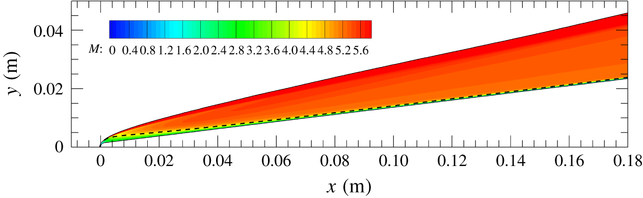
The Mach number contours of the laminar boundary-layer flow from table 1 are shown in figure 1. The streamwise domain shown in the figure includes both the nose tip and the transition location measured in the experiment ( $\unicode[STIX]{x1D709}_{T}=0.133~\text{m}$). The entropy-layer edge,
 $\unicode[STIX]{x1D6FF}_{S}$, is defined as the location where the local entropy increment is
 $0.25$ times the entropy increment at the wall (
 $\unicode[STIX]{x0394}S(\unicode[STIX]{x1D709},\unicode[STIX]{x1D702}=\unicode[STIX]{x1D6FF}_{S})=0.25\unicode[STIX]{x0394}S_{wall}$). The entropy increment,
 $\unicode[STIX]{x0394}S$, is defined with respect to the free-stream value, i.e.
 $\unicode[STIX]{x0394}S=c_{p}\text{ln}(\bar{T}/\bar{T}_{\infty })-R_{g}\text{ln}(\bar{p}/\bar{p}_{\infty })$, where
 $c_{p}=1004~\text{J}~\text{kg}^{-1}~\text{K}^{-1}$ is the specific heat for a constant pressure and
 $R_{g}=287.058~\text{J}~\text{kg}^{-1}~\text{K}^{-1}$ is the specific gas constant. The entropy-layer edge approaches the boundary-layer edge as the streamwise location increases. The local Mach number remains below approximately 4.4 under the entropy-layer edge.
Mach number ( $M$) contours of the laminar boundary-layer flow over a
 $7^{\circ }$ half-angle circular cone with
 $R_{N}=1.524~\text{mm}$ and conditions shown in table 1. The dashed, black line indicates the edge of the entropy layer,
 $\unicode[STIX]{x1D6FF}_{S}$.

3.2 Linear disturbance evolution
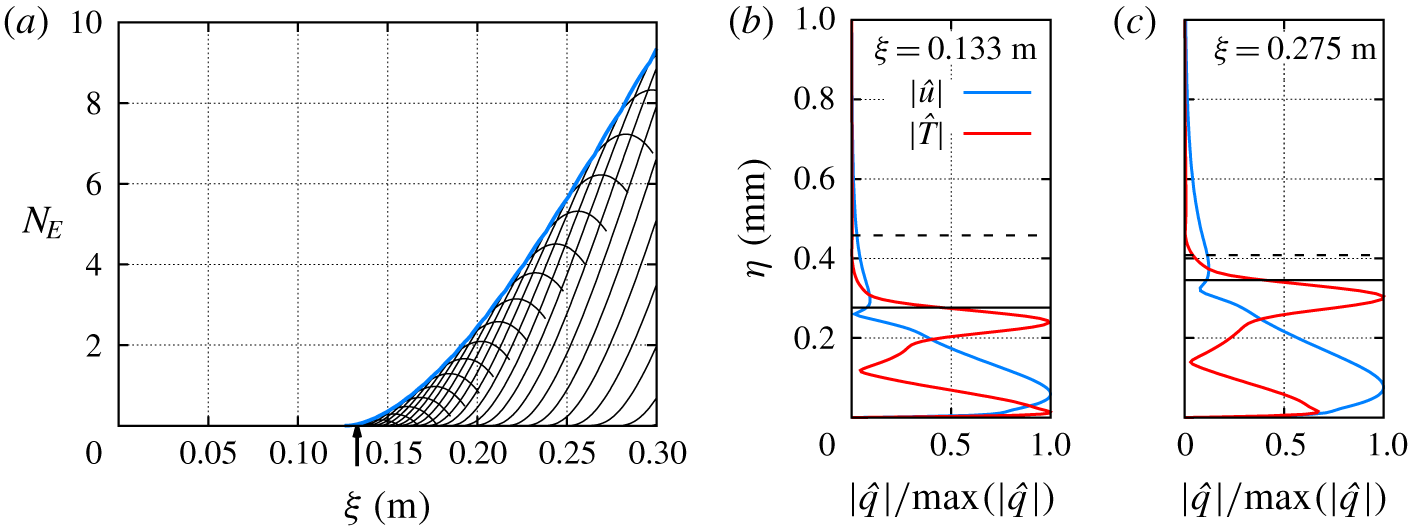
A detailed modal instability analysis of the present configuration was performed by Jewell et al. (Reference Jewell, Kennedy, Laurence and Kimmel2018) and Paredes et al. (Reference Paredes, Choudhari, Li, Jewell and Kimmel2019c) at the flow condition of interest and only Mack-mode instabilities had positive growth rates in this case. All entropy-layer modes and first-mode instabilities were found to be damped. Figure 2(a) shows the  $N$-factor curves of planar Mack-mode waves based on total energy
 $E$,
 $N_{E}=1/2\,\log (E(\unicode[STIX]{x1D709}_{1})/E(\unicode[STIX]{x1D709}_{0}))$, where we have used the energy norm derived by Chu (Reference Chu1956) and used by Mack (Reference Mack1969) for linear stability theory. This energy norm is defined as
 $$\begin{eqnarray}E(\unicode[STIX]{x1D709})=\int _{\unicode[STIX]{x1D702}}\hat{\boldsymbol{q}}(\unicode[STIX]{x1D709},\unicode[STIX]{x1D702})^{H}\boldsymbol{M}_{E}\,\hat{\boldsymbol{q}}(\unicode[STIX]{x1D709},\unicode[STIX]{x1D702})\,h_{\unicode[STIX]{x1D709}}\,h_{\unicode[STIX]{x1D701}}\,\text{d}\unicode[STIX]{x1D702},\end{eqnarray}$$
where the superscript  $H$ denotes conjugate transpose and
 $\boldsymbol{M}_{E}$ is the energy weight matrix,
 $$\begin{eqnarray}\boldsymbol{M}_{E}=\text{diag}\left[\frac{\bar{T}(\unicode[STIX]{x1D709},\unicode[STIX]{x1D702})}{\unicode[STIX]{x1D6FE}\bar{\unicode[STIX]{x1D70C}}(\unicode[STIX]{x1D709},\unicode[STIX]{x1D702})M^{2}},\bar{\unicode[STIX]{x1D70C}}(\unicode[STIX]{x1D709},\unicode[STIX]{x1D702}),\bar{\unicode[STIX]{x1D70C}}(\unicode[STIX]{x1D709},\unicode[STIX]{x1D702}),\bar{\unicode[STIX]{x1D70C}}(\unicode[STIX]{x1D709},\unicode[STIX]{x1D702}),\frac{\bar{\unicode[STIX]{x1D70C}}(\unicode[STIX]{x1D709},\unicode[STIX]{x1D702})}{\unicode[STIX]{x1D6FE}(\unicode[STIX]{x1D6FE}-1)\bar{T}(\unicode[STIX]{x1D709},\unicode[STIX]{x1D702})M^{2}}\right].\end{eqnarray}$$
For the present configuration, the Mack-mode instability becomes unstable slightly upstream of the measured transition location  $\unicode[STIX]{x1D709}_{T}=0.133~\text{m}$, resulting in a rather small peak N-factor of
 $N_{E}(\unicode[STIX]{x1D709}_{T})=0.04$ for a disturbance frequency of
 $f=1320~\text{kHz}$. For sharp cone configurations, an amplification factor of
 $N_{E}=7.5$ was found to correlate with the onset of Mack-mode dominated transition in the same facility (Jewell & Kimmel Reference Jewell and Kimmel2017; Jewell et al. Reference Jewell, Kennedy, Laurence and Kimmel2018). In the present case, the latter value of Mack-mode
 $N$-factor would be achieved at
 $\unicode[STIX]{x1D709}=0.275~\text{m}$ by a planar Mack-mode disturbance at
 $f=1020~\text{kHz}$. Therefore, the Mack-mode instability cannot be the cause of transition at
 $\unicode[STIX]{x1D709}=0.133~\text{m}$ as measured during the experiments by Jewell et al. (Reference Jewell, Kennedy, Laurence and Kimmel2018). The mode shapes for the magnitudes of streamwise velocity and temperature fluctuations associated with the Mack-mode disturbances corresponding to
 $f=1320~\text{kHz}$ at
 $\unicode[STIX]{x1D709}=0.133~\text{m}$ and to
 $f=1020~\text{kHz}$ at
 $\unicode[STIX]{x1D709}=0.275~\text{m}$ are shown in figures 2(b) and 2(c), respectively. Both disturbance profiles are mostly contained below the boundary-layer edge.
Given the absence of a significant modal growth up to the measured transition location, the transient growth mechanism was investigated as a potential cause for the onset of transition by Paredes et al. (Reference Paredes, Choudhari, Li, Jewell, Kimmel, Marineau and Grossir2018, Reference Paredes, Choudhari, Li, Jewell, Kimmel, Marineau and Grossir2019d,Reference Paredes, Choudhari, Li, Jewell and Kimmelc). Their linear optimal growth analysis showed appreciable non-modal growth over the streamwise interval of  $(\unicode[STIX]{x1D709}_{0},\unicode[STIX]{x1D709}_{1})=(0.014,0.133)~\text{m}$ that precedes the measured transition location at
 $\unicode[STIX]{x1D709}_{1}=\unicode[STIX]{x1D709}_{T}=0.133~\text{m}$. The highest logarithmic energy gain of
 $N_{E}=5.58$ occurred for an oblique stationary disturbance with
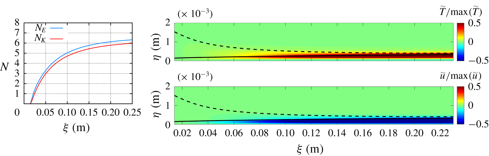
 $m=68$, and the perturbations associated with this mode are mostly confined to the boundary-layer region as seen in figure 3, where the
 $N$-factor curves based on the total and kinetic energies and the evolution of the temperature and streamwise velocity fluctuations of such oblique stationary disturbance (
 $f=0~\text{kHz}$ and
 $m=68~\text{m}$) are shown.
(a) The  $N$-factor curves for planar Mack-mode instability with disturbance frequencies in the range of
 $f=820-1340~\text{kHz}$. The vertical arrow indicates the measured transition location at
 $\unicode[STIX]{x1D709}_{T}=0.133~\text{m}$. Also, normalized profiles of streamwise velocity and temperature disturbance components for (b)
 $f=1320~\text{kHz}$ at
 $\unicode[STIX]{x1D709}=0.133~\text{m}$ and (c)
 $f=1020~\text{kHz}$ at
 $\unicode[STIX]{x1D709}=0.275~\text{m}$. The solid and dashed black lines indicate the edge of the boundary layer,
 $\unicode[STIX]{x1D6FF}_{h}$, and the edge of the entropy layer,
 $\unicode[STIX]{x1D6FF}_{S}$, respectively.

Evolution of  $N$-factor based on total energy (
 $N_{E}$) and kinetic energy (
 $N_{K}$), and contours of normalized temperature and streamwise velocity components of the optimal perturbation for an oblique stationary disturbance with
 $(F,m)=(0~\text{kHz},m=68)$. The solid and dashed black lines indicate the edge of the boundary layer,
 $\unicode[STIX]{x1D6FF}_{h}$, and the edge of the entropy layer,
 $\unicode[STIX]{x1D6FF}_{S}$, respectively.

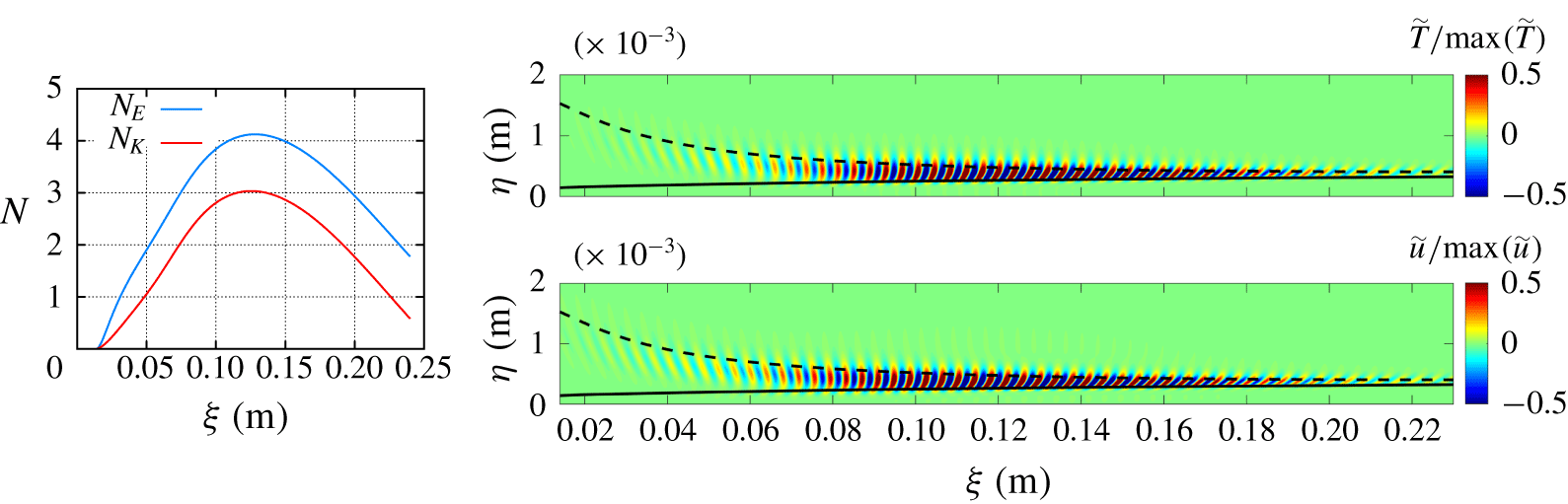
Evolution of  $N$-factor based on total energy (
 $N_{E}$) and kinetic energy (
 $N_{K}$), and contours of normalized temperature and streamwise velocity components of the optimal perturbation for an oblique travelling disturbance with
 $(F,m)=(250~\text{kHz},m=50)$. The solid and dashed black lines indicate the edge of the boundary layer,
 $\unicode[STIX]{x1D6FF}_{h}$, and the edge of the entropy layer,
 $\unicode[STIX]{x1D6FF}_{S}$, respectively.

Even though stationary disturbances of this type may be preferentially excited on a rough surface, they are not believed to be the primary cause for transition over moderately blunt cones with polished surfaces, as mentioned in the Introduction. The optimal energy gain becomes smaller as the frequency is increased above zero; however, a qualitative change is noted when the frequency parameter becomes sufficiently large. Specifically, the disturbance structure of the travelling disturbances is rather different from that of the stationary streaks underlying linear optimal growth as shown in figure 3. Figure 4 shows the  $N$-factor curves based on the total and kinetic energies and the evolution of the temperature and streamwise velocity fluctuations of a three-dimensional travelling disturbance with
 $f=250~\text{kHz}$ and
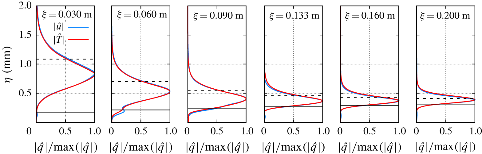
 $m=50$. Figure 5 shows the profiles at selected streamwise locations of the same disturbance plotted in figure 4. The distribution of the profiles confirms that most of the disturbance energy is contained in between the edges of the boundary layer and the entropy layer, and has a weak signature within the boundary-layer region (i.e. below the boundary-layer edge). The peak
 $N$-factor based on the energy norm from (3.1) is
 $N_{E}=4.13$, which is lower than the peak
 $N$-factor associated with stationary disturbances (
 $N_{E}=5.58$), but only by a small extent. More important, the growth in thermodynamic fluctuations plays an increasingly important role in the linear transient growth of the travelling disturbance. In particular, the
 $N$-factor based on the kinetic energy of the disturbance is lower than that based on the overall energy norm (
 $N_{E}=4.13$) by approximately
 $\unicode[STIX]{x0394}N\approx 1.1$. In contrast, the difference in
 $N$-factors for the dominant stationary disturbance with
 $m=68$ is rather small,
 $\unicode[STIX]{x0394}N\approx 0.33$. The linear, non-modal growth analysis by Paredes et al. (Reference Paredes, Choudhari, Li, Jewell and Kimmel2019c) indicated an additional, secondary peak in the energy gain contours within the
 $m=0$ axis of the frequency–azimuthal wavenumber plane. This secondary peak corresponds to
 $N_{E}=3.6$, which occurs for planar disturbances with
 $f=420~\text{kHz}$. However, the frequency bandwidth of the secondary peak is quite large, such that planar disturbances with frequencies between 300 kHz and 850 kHz experience an energy amplification factor in the narrow range of
 $N_{E}=(3.5,3.6)$. Although not shown, the planar travelling disturbances also have a weak signature within the boundary-layer region.
Normalized profiles of streamwise velocity and temperature disturbance components of the optimal perturbation for an oblique travelling disturbance with  $(F,m)=(250~\text{kHz},m=50)$ at selected streamwise locations. The solid and dashed black lines indicate the edge of the boundary layer,
 $\unicode[STIX]{x1D6FF}_{h}$, and the edge of the entropy layer,
 $\unicode[STIX]{x1D6FF}_{S}$, respectively.

3.3 Nonlinear evolution of non-modal oblique travelling disturbances
The linear optimal growth analysis for travelling disturbances has shown that oblique disturbances in the entropy layer can achieve significantly larger energy gain than the planar travelling disturbances. However, the process of boundary-layer transition to turbulence involves the generation of self-sustaining eddies near the wall. Thus, without a mechanism for the disturbances to penetrate from the entropy layer into the boundary-layer region, the role of the oblique travelling disturbances undergoing a relatively large non-modal growth remains unclear. We now investigate whether nonlinear interactions can provide that mechanism.
For the nonlinear computations, the five components  $(\tilde{\unicode[STIX]{x1D70C}},\tilde{u} ,\tilde{v},\tilde{w},\tilde{T})$ of the linear non-modal disturbance field from figure 4 are extracted at the inflow location of
 $\unicode[STIX]{x1D709}=0.03~\text{m}$. Specifically, an inflow disturbance composed of a pair of oblique travelling waves with
 $f=250$ kHz and
 $m=\pm 50$ is used to investigate the possibility of oblique-mode breakdown. The salient features of oblique-mode breakdown involving linearly unstable modes have been reported both for incompressible boundary layers (where the nonlinear interaction between a pair of oblique Tollmien–Schlichting waves (Berlin, Lundbladh & Henningson Reference Berlin, Lundbladh and Henningson1994) drives the breakdown process) and for supersonic boundary layers (that involve the interaction between a pair of oblique first-mode waves (Thumm Reference Thumm1991; Joslin, Streett & Chang Reference Joslin, Streett, Chang, Hussaini, Kumar and Streett1992; Adams & Kleiser Reference Adams, Kleiser, Kral and Zang1993; Fasel, Thumm & Bestek Reference Fasel, Thumm, Bestek, Kral and Zang1993; Chang & Malik Reference Chang and Malik1994; Laible, Mayer & Fasel Reference Laible, Mayer and Fasel2009; Mayer, Von Terzi & Fasel Reference Mayer, Von Terzi and Fasel2011; Laible & Fasel Reference Laible and Fasel2016; Panina et al. Reference Panina, Kosinov, Semionov and Yermolaev2017) and between a pair of oblique Mack-mode waves (Sivasubramanian & Fasel Reference Sivasubramanian and Fasel2013)). The present oblique-mode breakdown differs from the aforementioned cases because it is initiated by the interaction between a pair of oblique travelling waves that peak within the entropy layer beyond the boundary-layer edge. Finally, the effect of the initial amplitude and the frequency and azimuthal wavenumber of the inflow disturbances is also analysed. A peak root-mean-square initial amplitude of
 $\tilde{u} _{rms}/u_{\infty }=u_{0,b}=1.0087\times 10^{-3}$ is used as the baseline case for the following parametric study.
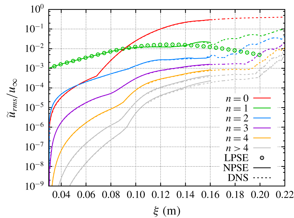
Root-mean-square evolution of streamwise velocity disturbance computed with NPSE and DNS for a fundamental disturbance composed of a pair of travelling waves with  $f=250~\text{kHz}$ and
 $m=\pm 50$ with an initial amplitude of
 $\tilde{u} _{rms}/u_{\infty }=u_{0,b}$. The linear evolution of the fundamental mode computed with LPSE is also included.

Figure 6 shows the streamwise evolution of the root-mean-square of the streamwise velocity disturbance corresponding to the fundamental frequency ( $n=1$), the stationary mode (
 $n=0$) that includes both the mean-flow-distortion (MFD) and the three-dimensional wavelengths
 $m\neq 0$, and the non-stationary harmonics (
 $n>0$) created via nonlinear effects. For clarity, higher harmonics beyond
 $n=6$ are not shown in the plot, because the amplitude of the harmonic decreases with increasing mode index. For example, the amplitude of the harmonic corresponding to
 $n=7$ is 3–4 orders of magnitude lower than the amplitude of the fundamental Fourier component (
 $n=1$). Good agreement is observed between the three methodologies, but the nonlinear predictions begin to deviate from the linear curve around
 $\unicode[STIX]{x1D709}=0.1~\text{m}$. From this location, the nonlinear effects become appreciable, but the NPSE and DNS continue to agree, with the exception of minor discrepancies for the higher harmonics. However, as the disturbance amplitude becomes sufficiently large, the NPSE marching fails to converge, starting at approximately
 $\unicode[STIX]{x1D709}=0.16~\text{m}$. The stationary mode experiences a rapid growth starting from
 $\unicode[STIX]{x1D709}\approx 0.07~\text{m}$. This abrupt change in the slope of the stationary-mode amplitude curve is caused by a switchover in the peak location of the MFD profile, from an outer peak in the entropy layer upstream of
 $\unicode[STIX]{x1D709}\approx 0.07~\text{m}$ to an inner peak within the boundary-layer region for
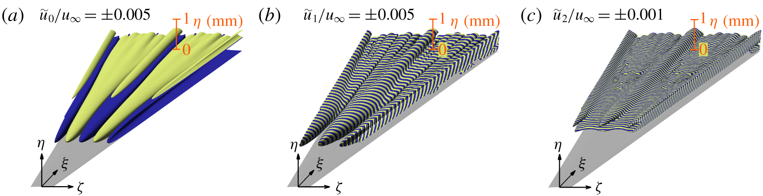
 $\unicode[STIX]{x1D709}>0.07~\text{m}$. Figures 7(a), 7(b) and 7(c) show three-dimensional views of the isosurfaces of streamwise velocity disturbance for the stationary, fundamental and first harmonic modes, respectively. The fundamental mode peaks within the entropy layer at a sufficient upstream location, i.e. significantly farther out from the boundary-layer edge, but the peak location approaches the boundary-layer edge with an increasing downstream distance. The emergence of the stationary streaks associated with the stationary mode coincides with the axial location where the peak fundamental fluctuations approach the edge of the mean boundary layer from above. The stationary streaks, also referred to as the longitudinal or streamwise vortex mode in oblique-mode transition studies (e.g. Schmid & Henningson Reference Schmid and Henningson1992; Berlin et al. Reference Berlin, Lundbladh and Henningson1994; Chang & Malik Reference Chang and Malik1994), increase in amplitude along the downstream direction, as the result of a continuously forced transient growth mechanism (Laible & Fasel Reference Laible and Fasel2016). The evolution of boundary-layer streaks in the present computation shares some similarities with the studies of Siconolfi, Camarri & Fransson (Reference Siconolfi, Camarri and Fransson2015) and Martin & Paredes (Reference Martin and Paredes2016), where a pair of stationary vortices are introduced in an incompressible flat-plate boundary-layer flow at selected distances from the boundary-layer edge to study the generation of stationary streaks and their attenuation effect on Tollmien–Schlichting waves. However, it also different from those works in that those prior studies already involved a stationary forcing, whereas the input forcing in the present case corresponds to travelling disturbances and the stationary streaks are produced via the nonlinear interaction between those travelling disturbances. The nonlinear streak generation mechanism is also different from the generation of low-frequency Klebanoff modes excited by free-stream turbulence (Andersson, Berggren & Henningson Reference Andersson, Berggren and Henningson1999; Leib, Wundrow & Goldstein Reference Leib, Wundrow and Goldstein1999; Ovchinnikov, Choudhari & Piomelli Reference Ovchinnikov, Choudhari and Piomelli2008). The continued amplification of stationary streaks leads to a strong azimuthal modulation of the boundary-layer flow. Disturbances at the first harmonic (
 $n=2$, i.e.
 $f=500~\text{kHz}$) of the fundamental disturbance are initially dominated by the axisymmetric wave created by the nonlinear interaction between the pair of oblique waves at the fundamental frequency of
 $f=250~\text{kHz}$. Farther downstream, however, the disturbance motion at all three leading frequencies (i.e. stationary, fundamental and the first harmonic) develop a more complex structure, which involves an azimuthal modulation of the initial axisymmetric disturbance at
 $f=500~\text{kHz}$ by the stationary streaks as well as the appearance of higher harmonics in the azimuthal direction.
Positive (blue) and negative (yellow) isosurfaces of streamwise velocity disturbance of (a) stationary ( $n=0$), (b) fundamental (
 $n=1$) and (c) first harmonic (
 $n=2$) modes computed with DNS for an initial disturbance composed of a pair of travelling waves with
 $F=250~\text{kHz}$ and
 $m=\pm 50$ with an initial amplitude of
 $\tilde{u} _{rms}/u_{\infty }=u_{0,b}$. The plotted spatial domain corresponds to a single azimuthal wavelength of the fundamental mode (
 $\unicode[STIX]{x1D706}=2\unicode[STIX]{x03C0}/50$) for a streamwise domain of
 $\unicode[STIX]{x1D709}\in [0.03,0.22]~\text{m}$.

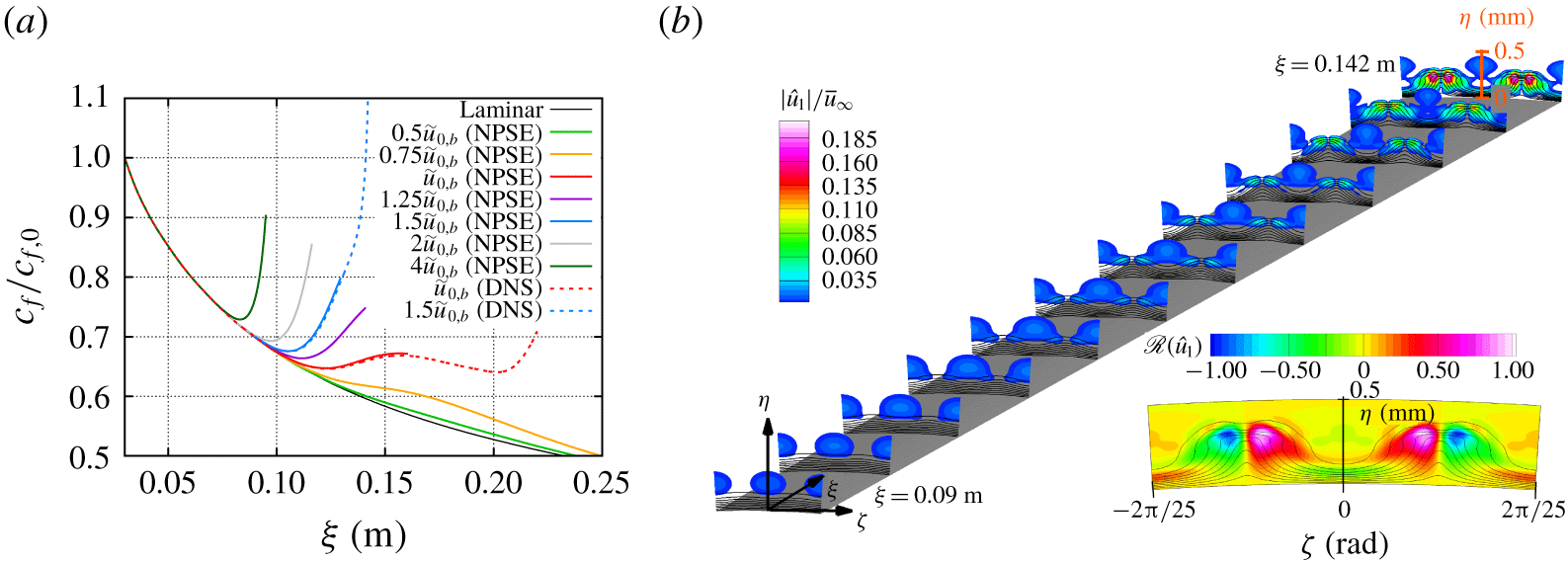
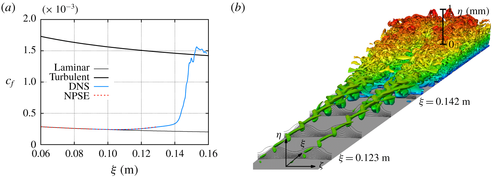
(a) Evolution of the normalized skin friction coefficient for the nonlinear evolution of an initial disturbance composed of a pair of travelling waves with  $f=250~\text{kHz}$ and
 $m=\pm 50$ with selected initial amplitudes. (b) Streamwise velocity magnitude isocontours of the fundamental mode and streamwise velocity isolines of the time averaged flow (i.e. superposition of the basic state and the stationary mode) based on the DNS for an initial amplitude of
 $\tilde{u} _{rms}/u_{\infty }=1.5u_{0,b}$. The plotted spatial domain corresponds to a single azimuthal wavelength of the fundamental mode (
 $\unicode[STIX]{x1D706}=2\unicode[STIX]{x03C0}/50$) for a streamwise domain of
 $\unicode[STIX]{x1D709}\in [0.09,0.142]~\text{m}$. Also, the normalized isocontours of the real part of streamwise velocity of the fundamental mode with the streamwise velocity isolines of the superposition of the basic flow and the stationary mode is shown at
 $\unicode[STIX]{x1D709}=0.142~\text{m}$.

Figure 8(a) shows the evolution of the skin friction coefficient for the laminar basic state and for selected initial amplitudes. The NPSE is used to determine the initial amplitude that would lead to transition onset at the measured location of  $\unicode[STIX]{x1D709}_{T}=0.133$ m (Jewell et al. Reference Jewell, Kennedy, Laurence and Kimmel2018). DNS results are shown for initial amplitudes equal to
 $u_{0,b}$ and
 $1.5u_{0,b}$. The NPSE and DNS skin friction predictions agree until the PSE marching fails to converge. Although not shown here, equivalent results are found for the heat transfer coefficient. The NPSE method is able to reach the initial rise in the skin friction and heat transfer coefficients, in close agreement with the DNS prediction. Therefore, NPSE provides an efficient technique for the parametric study of the early phase of the nonlinear development of this type of non-modal travelling disturbances, up to and somewhat beyond the initial rise in skin friction caused by the stationary streaks from the stationary mode. The DNS and NPSE results of figure 8(a) show that the skin friction for the case with an initial amplitude of
 $u_{0,b}$ reaches a local maximum at approximately
 $\unicode[STIX]{x1D709}=0.16~\text{m}$. From this location, the NPSE fails to converge, but the DNS results show a weak transient decay until
 $\unicode[STIX]{x1D709}\approx 0.205~\text{m}$, followed by a second rise in skin friction (and heat transfer) as a result of streak breakdown. The transient decay in skin friction and heat transfer observed for an initial amplitude of
 $u_{0,b}$ is due to the slow growth of the streak instabilities for this particular case that prolongs the beginning of the streak breakdown until
 $\unicode[STIX]{x1D709}\approx 0.205~\text{m}$. However, the skin friction curve for the higher initial amplitude of
 $1.5u_{0,b}$ exhibits an increased slope at
 $\unicode[STIX]{x1D709}\approx 0.14~\text{m}$. Figure 8(b) shows the isolines of the stationary streamwise velocity corresponding to the superposition of the unperturbed, laminar basic state and stationary mode, together with the isocontours of the fundamental mode for the
 $1.5u_{0,b}$ initial amplitude case. Both sets of contours clearly highlight the azimuthal modulation of the boundary layer due to the finite-amplitude streaks at twice the azimuthal wavenumber of the primary, travelling mode disturbance. Furthermore, the streaks become unstable and the disturbance at the fundamental frequency becomes a subharmonic sinuous streak instability. Here, the subharmonic nature refers to the subharmonic azimuthal wavelength of the disturbance (
 $m=50$) with respect to the streak wavelength (
 $m=100$), as shown by the contours of the real part of the streamwise velocity corresponding to the fundamental mode in the figure 8(b). This sinuous disturbance increases in amplitude and eventually leads to a breakdown of the streaks. Simultaneously, as the disturbance amplitude begins to increase close to the wall, a higher slope of the skin friction curve is observed in figure 8(a). At the further downstream locations, the disturbance amplitude begins to increase close to the wall, leading to the higher slope of the skin friction curve as observed in figure 8(a).
Recent studies have shown that under certain set of parameters, stationary streaks can stabilize oblique first-mode waves in supersonic boundary-layer flows (Paredes et al. Reference Paredes, Choudhari and Li2017; Sharma et al. Reference Sharma, Shadloo, Hadjadj and Kloker2019) and Mack-mode waves in hypersonic boundary-layer flows (Paredes, Choudhari & Li Reference Paredes, Choudhari and Li2019a). However, at large enough amplitudes, the same streaks are able to induce transition via streak instabilities (Paredes et al. Reference Paredes, Choudhari and Li2017, Reference Paredes, Choudhari and Li2019a). The eventual breakdown in the present flow configuration resembles the latter scenario as seen from the threshold initial amplitudes between  $0.75u_{0,b}$ and
 $u_{0,b}$ in figure 8(a).
Streamwise velocity isocontours of the non-stationary perturbations ( $n>0$) and streamwise velocity isolines of the superposition of the basic flow and the stationary mode computed with DNS at (a)
 $\unicode[STIX]{x1D709}=0.1365~\text{m}$, (b)
 $\unicode[STIX]{x1D709}=0.1408~\text{m}$, (c)
 $\unicode[STIX]{x1D709}=0.1444~\text{m}$, (d)
 $\unicode[STIX]{x1D709}=0.1473~\text{m}$, (e)
 $\unicode[STIX]{x1D709}=0.1498~\text{m}$ and (f)
 $\unicode[STIX]{x1D709}=0.1522~\text{m}$ for an initial amplitude of
 $\tilde{u} _{rms}/u_{\infty }=1.5u_{0,b}$. The plotted spatial domain corresponds to a single azimuthal wavelength of the fundamental mode (
 $\unicode[STIX]{x1D706}=2\unicode[STIX]{x03C0}/50$). The aspect ratio between vertical and horizontal scales is one.

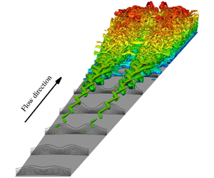
(a) Evolution of the skin friction coefficient and (b) Q-criterion isosurfaces coloured by the distance to the wall with streamwise velocity isolines at selected cross-planes of the instantaneous flow field for the nonlinear evolution of an initial disturbance composed of a pair of travelling waves with  $f=250~\text{kHz}$ and
 $m=\pm 50$ with an initial amplitude of
 $\tilde{u} _{rms}/u_{\infty }=1.5u_{0,b}$. The plotted spatial domain of subfigure (b) corresponds to a single azimuthal wavelength of the fundamental mode (
 $\unicode[STIX]{x1D706}=2\unicode[STIX]{x03C0}/50$) for a streamwise domain of
 $\unicode[STIX]{x1D709}\in [0.09,0.159]~\text{m}$. The turbulent prediction is calculated with van Driest II model for cold wall conditions.

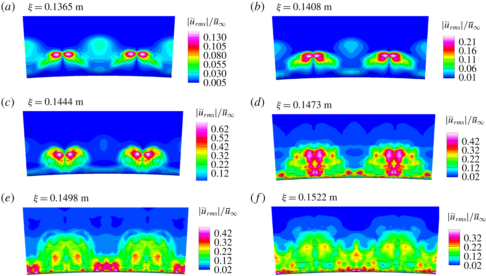
Figure 9 shows the isocontours of streamwise velocity fluctuations comprised of the dominant Fourier harmonics corresponding to  $n=1$ to
 $11$, together with the isolines of the superposition of the laminar basic state and the stationary mode at selected streamwise locations in the region of laminar flow breakdown. The disturbance amplitude increases from
 $\unicode[STIX]{x1D709}=0.1365~\text{m}$ (figure 9a) to
 $\unicode[STIX]{x1D709}=0.1444~\text{m}$ (figure 9c) as the locations of peak velocity fluctuation remain significantly above the wall and azimuthally close to the crest of the streaks (i.e. the azimuthal region with larger boundary-layer thickness). At around
 $\unicode[STIX]{x1D709}=0.1473~\text{m}$ (figure 9d), the peak magnitude of the fluctuations is reduced with respect to the preceding location, but additional peaks have developed closer to the wall, but still under the crest of the streaks. Even further downstream at
 $\unicode[STIX]{x1D709}=0.1498~\text{m}$ (figure 9e) and
 $\unicode[STIX]{x1D709}=0.1522~\text{m}$ (figure 9f), the peak fluctuations have shifted to the valley of the streaks, where the boundary layer is thinner, but the fluctuation levels as well as the boundary-layer thickness have become more homogeneous along the azimuthal direction indicating that the transition process is nearly complete. Figure 10(a) shows that the dominance of near-wall fluctuations near
 $\unicode[STIX]{x1D709}\gtrsim 0.15~\text{m}$, is accompanied by the mean skin friction approaching the prediction for a fully turbulent boundary layer based on the van Driest II model (van Driest Reference van Driest1956). The mean skin friction at the downstream locations is nearly
 $8$ times larger than the laminar friction coefficient. Figure 10(b) shows the instantaneous Q-criterion isosurfaces, together with the streamwise velocity isolines, at selected streamwise locations. The isosurface evolution in this figure further illustrates the nature of the transition process discussed so far. The breakdown process is initiated by the amplification of a subharmonic sinuous instability. Vortical structures emerge close to the wall for
 $\unicode[STIX]{x1D709}>0.14~\text{m}$ and lead to transition onset. Overall, the results discussed in this section indicate that transition onset near the measured location of
 $\unicode[STIX]{x1D709}_{T}=0.133~\text{m}$ can occur as a result of the nonlinear interactions initiated by a pair of oblique non-modal travelling waves, even in the absence of any modal growth associated with the first-mode or Mack-mode instabilities.
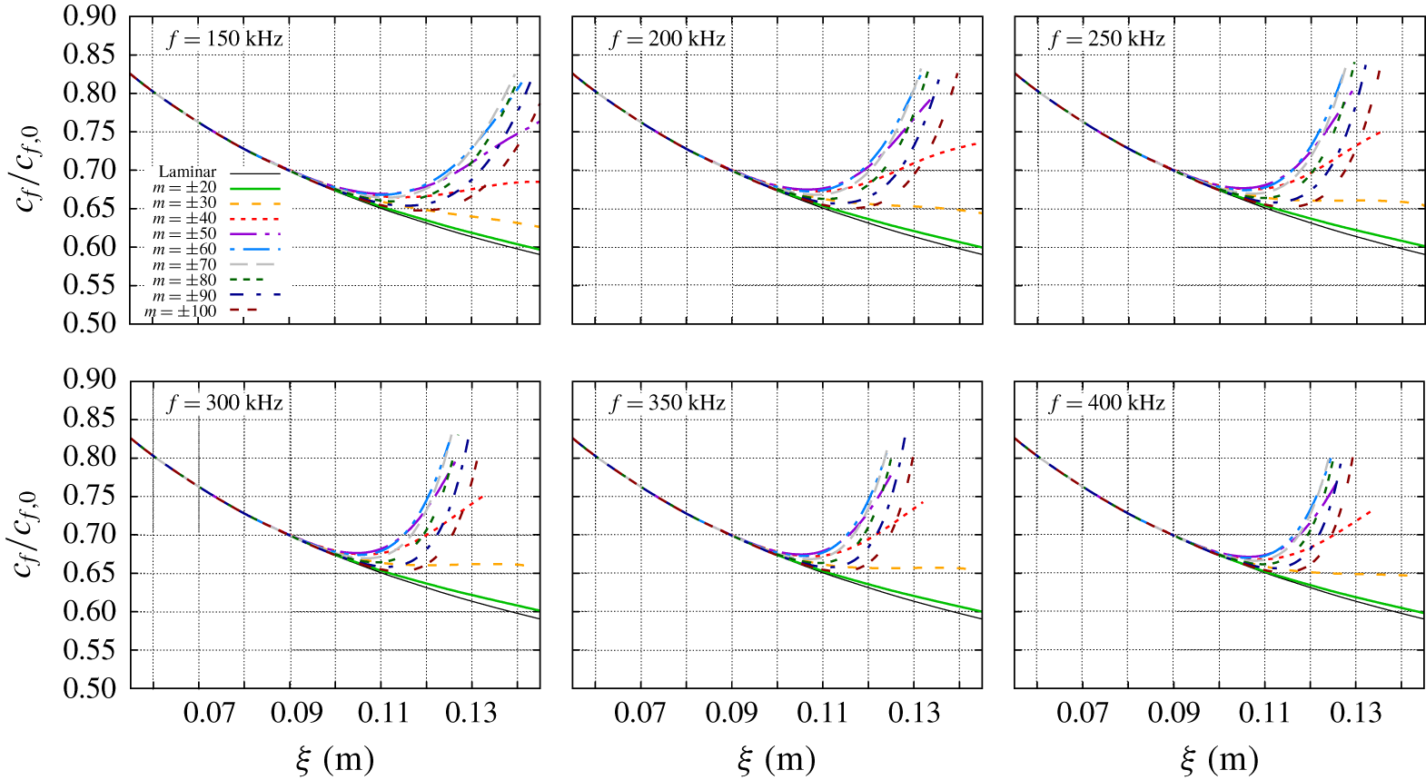
Evolution of the skin friction coefficient for the nonlinear evolution of an initial disturbance composed of a pair of travelling waves with  $f=(150:50:400)~\text{kHz}$ and
 $m=\pm (20:10:100)$ with an initial amplitude of
 $\tilde{u} _{rms}/u_{\infty }=1.5u_{0,b}$.

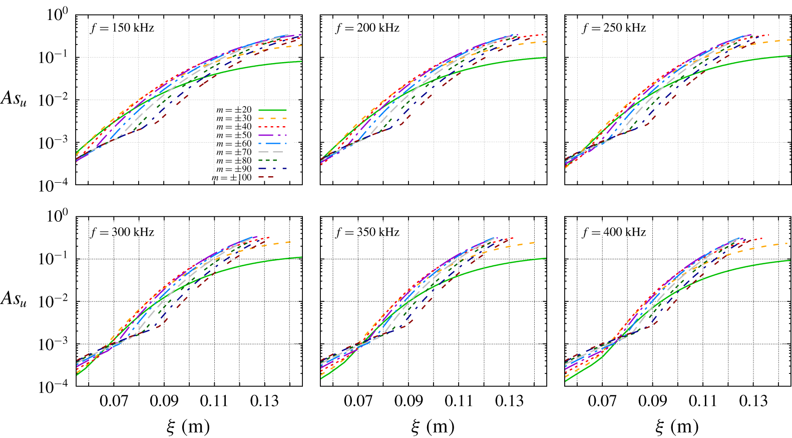
Evolution of the streak amplitude for the nonlinear evolution of an initial disturbance composed of a pair of travelling waves with  $f=(150:50:400)~\text{kHz}$ and
 $m=\pm (20:10:100)$ with an initial amplitude of
 $\tilde{u} _{rms}/u_{\infty }=1.5u_{0,b}$.

Finally, the effect of the frequency and azimuthal wavelength of the fundamental oblique pair of travelling waves is analysed. Figures 11 and 12 show the evolution of the skin friction coefficients and streak amplitudes of the stationary mode computed with NPSE with a fixed initial amplitude of  $1.5u_{0,b}$ for fundamental frequencies equal to
 $f=150$,
 $200$,
 $250$,
 $300$,
 $350$ and
 $400~\text{kHz}$ and azimuthal wavenumbers from
 $m=\pm 20$ to
 $m=\pm 100$ in increments of
 $10$. The streak amplitude is based on the streamwise velocity perturbation of the stationary mode as
 $$\begin{eqnarray}As_{u}(\unicode[STIX]{x1D709})={\textstyle \frac{1}{2}}[\text{max}_{\unicode[STIX]{x1D702},\unicode[STIX]{x1D701}}(\tilde{u} _{0}(\unicode[STIX]{x1D709},\unicode[STIX]{x1D702},\unicode[STIX]{x1D701}))-\min _{\unicode[STIX]{x1D702},\unicode[STIX]{x1D701}}(\tilde{u} _{0}(\unicode[STIX]{x1D709},\unicode[STIX]{x1D702},\unicode[STIX]{x1D701}))].\end{eqnarray}$$
The results show that the inflow disturbances composed of a pair of oblique travelling waves are the most efficient in generating the stationary streaks for frequencies in the range of  $f=250{-}350~\text{kHz}$ and azimuthal wavenumbers of
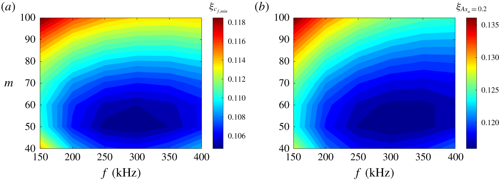
 $m=\pm (50{-}60)$, because, for a fixed initial amplitude of the inflow disturbances, the minimum in the skin friction coefficient appears earlier for these frequency–wavenumber pairs and higher streak amplitudes are reached at a given axial location. Of course, an earlier rise in skin friction does not imply the earliest completion of the laminar breakdown process. However, the results of figures 11 and 12 indicates that the frequency–wavenumber pair selected for the DNS is representative of the transition mechanism targeted in the present study.
The range of the most efficient combinations of frequency and azimuthal wavenumber is more clearly visible in figure 13(a), which shows the isocontours of the streamwise location corresponding to the minimum skin friction from the curves in figure 11. Furthermore, figure 13(b) shows the isocontours of the streamwise location corresponding to a streak amplitude of  $As_{u}=0.2$, which was found by Paredes et al. (Reference Paredes, Choudhari and Li2019a) to correspond to the critical value for the subharmonic, sinuous instability modes to become unstable for a similar circular cone configuration at a somewhat lower free-stream Mach number of
 $5.3$. Again, the same range of parameters in frequency and azimuthal wavenumber space is found to yield the streak amplitude of
 $As_{u}=0.2$ at an earlier streamwise station. Because inflow disturbances with a broad range of frequencies and azimuthal wavenumbers would contribute to a similar process of streak formation, an inflow disturbance composed of a broad spectrum of frequencies and azimuthal wavenumbers is likely to accelerate the transition process in comparison with a single pair of oblique travelling waves. Preliminary computations of oblique-mode interactions with an additional planar wave at the inflow suggest that the planar wave can accelerate the nonlinear growth of the oblique wave, and hence, contribute to the amplification of the stationary streaks; nonetheless, the qualitative nature of the streak breakdown process appears to remain the same. To facilitate a better understanding of the role of the input disturbance spectrum, detailed numerical simulations would be beneficial as a follow on to the present study.
Isocontours of streamwise location corresponding to (a) minimum skin friction and (b) streak amplitude of  $As_{u}=0.2$ for the nonlinear evolution of an initial disturbance composed of a pair of travelling waves with
 $f=(150:50:400)~\text{kHz}$ and
 $m=\pm (20:10:100)$ with an initial amplitude of
 $\tilde{u} _{rms}/u_{\infty }=1.5u_{0,b}$.

4 Summary and concluding remarks
The present paper has shown how the linear, non-modal optimal growth of oblique travelling disturbances can lead to laminar–turbulent transition in a hypersonic boundary layer over a blunt cone that transitions even in the absence of any significant modal amplification upstream of the transition location. The focus of this work has been the so-called moderately blunt regime (as against the large-bluntness regime corresponding to transition reversal), wherein the transition onset location moves downstream over the cone frustum as the bluntness parameter is increased and surface roughness is not believed to play an important role in initiating the transition process (Stetson Reference Stetson1983).
The specific blunt-cone configuration examined herein was a  $7^{\circ }$ half-angle cone with
 $R_{n}=1.524~\text{mm}$ that was tested at zero degrees angle of attack by Jewell et al. (Reference Jewell, Kennedy, Laurence and Kimmel2018) in the AFRL Mach
 $6$ High Reynolds number facility at a unit Reynolds number of
 $Re_{\infty }=91.5\times 10^{6}~\text{m}^{-1}$. In this case, the modal growth of Mack-mode waves at the measured transition location is negligible (
 $N\approx 0.04$). However, previous analysis of linear non-modal growth by Paredes et al. (Reference Paredes, Choudhari, Li, Jewell and Kimmel2019c) had established the possibility of a significant energy gain upstream of the measured transition location for both stationary streaks and planar and oblique travelling disturbances initiated near the nose tip. Transition mechanisms for stationary streaks in high-speed boundary layers have been described in previous works. However, because the peak fluctuations associated with the travelling non-modal disturbances occur outside the boundary-layer region, their role in initiating boundary-layer transition had remained unclear until now. In that regard, the present study represents the first work to propose and demonstrate a potential mechanism for blunt-cone transition via the non-modal amplification of travelling wave disturbances within the entropy layer.
NPSE and DNS were used to investigate the path to transition via a pair of oblique travelling waves with equal but opposite azimuthal wavenumbers of  $m=\pm 50$ and a disturbance frequency of
 $f=250~\text{kHz}$. The NPSE and DNS predictions were found to be in excellent agreement, demonstrating that the NPSE can provide an accurate and efficient technique for predicting the initial phase of nonlinear development of the above non-modal travelling disturbances, including the initial rise in skin friction and heat transfer. Results show that for a relatively modest initial amplitude of
 $\tilde{u} _{rms}/u_{\infty }\approx 1.5\times 10^{-3}$, the nonlinear interactions between entropy-layer disturbances lead to the generation of stationary streaks inside the boundary layer that facilitate the amplification of an azimuthally subharmonic sinuous disturbance, which, in turn, leads to a streak breakdown and a subsequent onset of transition near the location measured in the experiment. A parametric analysis was conducted with NPSE to identify the most efficient combination of disturbance frequency and azimuthal wavenumbers that would lead to an earlier transition onset for a fixed initial amplitude of the fundamental pair of oblique waves. The disturbances with frequencies in the range of
 $f=250{-}350~\text{kHz}$ and azimuthal wavenumbers of
 $m=\pm (50{-}60)$ were found to be the most efficient in generating the stationary streaks that lead to the initial rise in skin friction and heat transfer, and furthermore, can achieve a streak amplitude of 20 % that can support unstable subharmonic streak instabilities en route to the streak breakdown process (Paredes et al. Reference Paredes, Choudhari and Li2019a).
While the present results may provide a potential explanation for transition through an oblique-mode transition mechanism in blunt cones upstream of the entropy-layer swallowing location when the modal growth of Mack-mode disturbances is too weak, the origin of these non-modal travelling disturbances that peak within the entropy layer has not been addressed herein. Furthermore, we note that there may be other potential mechanisms for the onset of transition in the moderately blunt regime. In particular, Paredes et al. (Reference Paredes, Choudhari and Li2019b) have suggested an alternative potential path to transition via the secondary instability (Herbert Reference Herbert1988) of axisymmetric non-modal disturbances inside the entropy layer. However, further work is necessary to delineate such alternative possibilities as well as to establish their relevance in technological applications. It goes without saying that the dominant transition mechanisms in any given case would be a function of the upstream disturbance spectrum and, therefore, additional work is suggested to characterize that dependence. Investigations into the effects of a broadband disturbance spectrum would also shed some light on the significance of varicose streak instability in certain parts of the parameter space.
Acknowledgements
This research was sponsored by the NASA’s Hypersonic Technology Project (HTP). A portion of the computational resources supporting this work were provided by the NASA High-End Computing (HEC) Program through the NASA Advanced Supercomputing (NAS) Division at Ames Research Center. The authors would like to thank Drs Corke, Grossir, Jewell, Kennedy, Kimmel, King, Laurence, Marineau and Schneider, for technical discussions related to this topic.
Declaration of interests
The authors report no conflict of interest.