1 Introduction
Well-being, though lacking a universally agreed-upon definition, is commonly associated with factors such as good health, both physical and mental, positive social relationships, and access to basic needs. Recent research has identified climate as a significant determinant of self-reported happiness (Rehdanz and Maddison, Reference Rehdanz and Maddison2005; Maddison and Rehdanz, Reference Maddison and Rehdanz2011; Connolly, Reference Connolly2012). With anticipated climate change in the future (IPCC, Reference IPCC2021a), understanding how individuals are affected by temperature variations becomes crucial for managing induced behaviors, benefiting individuals, health professionals, and public authorities alike.
Abundant evidence underscores the impact of weather on various aspects of human life and society. Temperature levels have been shown to affect agricultural yields (Deschênes and Greenstone, Reference Deschênes and Greenstone2007), labor productivity (Somanathan et al., Reference Somanathan, Somanathan, Sudarshan and Tewari2021), time allocation (Graff Zivin and Neidell, Reference Graff Zivin and Neidell2014), and human health (Deschênes and Greenstone, Reference Deschênes and Greenstone2011). Furthermore, temperature has been linked to diverse forms of violent conflict and social instability (Burke et al., Reference Burke, González, Baylis, Heft-Neal, Baysan, Basu and Hsiang2018), interpersonal violence (Simister and Cooper, Reference Simister and Cooper2005; Sanz-Barbero et al., Reference Sanz-Barbero, Linares, Vives-Cases, González, López-Ossorio and Díaz2018; Xu et al., Reference Xu, Xiong, Abramson, Li and Guo2021), increased suicide rates (Takahashi, Reference Takahashi2017; Burke et al., Reference Burke, González, Baylis, Heft-Neal, Baysan, Basu and Hsiang2018; Gao et al., Reference Gao, Cheng, Duan, Xu, Bai, Zhang, Zhang, Wang, Zhang and Su2019) and crime rates (Ranson, Reference Ranson2014; Obradovich et al., Reference Obradovich, Tingley and Rahwan2018; Baysan et al., Reference Baysan, Burke, González, Hsiang and Miguel2019).
Recent studies have leveraged social media data to investigate an additional dimension of climate's impact on human life and well-being: its influence on individuals’ mood. Researchers have used various platforms, including blogs (Dodds and Danforth, Reference Dodds and Danforth2010), Facebook (Baylis et al., Reference Baylis, Obradovich, Kryvasheyeu, Chen, Coviello, Moro, Cebrian and Fowler2018), Snapchat (Jiang et al., Reference Jiang, Murrugara-Llerena, Bos, Liu, Shah, Neves and Barbieri2022), Chinese social media Weibo (Wang et al., Reference Wang, Obradovich and Zheng2020; Cheng et al., Reference Cheng, Yu, Xu, Manoli, Ren, Zhang, Liu, Yin, Zhao and Vejre2023), the Russian social network Odnoklassniki (Smetanin, Reference Smetanin2022), and X-Twitter data (Baylis et al., Reference Baylis, Obradovich, Kryvasheyeu, Chen, Coviello, Moro, Cebrian and Fowler2018; Stevens et al., Reference Stevens, Beggs, Graham and Chang2019; Baylis, Reference Baylis2020), among others.Footnote 1 This approach offers distinct advantages, such as public availability, high-frequency data, and the richness of non-structured data for diverse characterizations, in contrast to the more resource-intensive and time-consuming nature of collecting self-reported well-being data using surveys that has typically been employed in assessing the weather-sentiment link in previous studies.
In this paper, we use approximately 80 million geo-tagged tweets from Argentina spanning 2017–2022 to assess the impact of temperatures on expressed sentiments, our proxy for well-being. X-Twitter, with 368 million monthly active users globally as of December 2022, is a prevalent choice in social science research.Footnote 2 We employ text mining techniques to convert unstructured text data (i.e., tweets) into two quantitative estimators: sentiments and a social media aggression index, focusing on the use of profanities. We then analyze their relationship with daily temperature using non-linear fixed effects panel regressions, controlling for potential confounders.
It is important to stress that the concept of well-being varies across disciplines and even within psychology (Jarden and Roache, Reference Jarden and Roache2023). Traditionally, well-being assessment has relied on self-report questionnaires; however, recent approaches have shifted towards the automatic analysis of individuals’ social media expressions. A comprehensive literature review by Sametoğlu et al. (Reference Sametoğlu, Pelt, Eichstaedt, Ungar and Bartels2024), corroborated by similar studies (e.g., Luhmann, Reference Luhmann2017; Settanni et al., Reference Settanni, Azucar and Marengo2018), reveals that the association between these two data types yields an average correlation of  $r = 0.39$ (range:
 $r = 0.08$ to
 $0.85$, depending on the studies included in the meta-analysis). Notably, this correlation is similar to that observed between self-report survey scores and professional informants’ (e.g., psychologists’) reports. There is also evidence that the cross-sectional prediction of US county life satisfaction from X-Twitter exceeds the predictive power of per capita income (Jaidka et al., Reference Jaidka, Giorgi, Schwartz, Kern, Ungar and Eichstaedt2020). Consequently, sentiment expressions in social media are anticipated to reflect well-being with efficacy similar to that of other established information sources.
Our paper makes two primary contributions to the existing literature. Firstly, we present an estimation of how temperature influences well-being in Argentina. This case is particularly interesting, as no previous studies have linked sentiments expressed in Spanish on social media to weather in this context.Footnote 3 Existing evidence has predominantly centered on the United States, some European countries, China, and a few others, showcasing country-specific variations influenced by factors such as temperature, demographics, and adaptive capacities. For instance, sentiment responses in China resemble those in the US for heat but are attenuated for cold. In this regard, this study contributes to the external validity of a small but growing literature by providing evidence from a previously unstudied region. Secondly, we compare results derived from geo-tagged tweets to those from self-declared user localization, demonstrating the consistency of our findings, an aspect not previously explored in the literature.
The manuscript is structured as follows: Section 2 provides a review of closely related studies. Section 3 details the construction of our database and outlines the empirical methodology. Section 4 discusses the results and their robustness, while section 5 presents the conclusion and policy implications.
2 Related literature
Social media information has been used across various fields, including sentiment analysis, popularity predictions, detection of public health phenomena such as the evolution of COVID-19, predictive changes in finance or product sales, and the detection of traffic accidents, among many others (Cano-Marin et al., Reference Cano-Marin, Mora-Cantallops and Sánchez-Alonso2023). This surge of applied work using social media data stems from a primary advantage of this information, that is, its ability to capture individual perceptions in a less time-consuming, intrusive, and costly manner compared to surveys, although it is not without challenges. These challenges include biases stemming from individuals’ self-selection on social media, occasional limitations in data accessibility, and the need to interpret unstructured data.
The use of social media data is revolutionizing research on human interactions with the environment and natural disasters management (Ghermandi et al., Reference Ghermandi, Langemeyer, Van Berkel, Calcagni, Depietri, Vigl, Fox, Havinga, Jöger and Kaiser2023). The topics studied are diverse, ranging from eco-tourists’ interests and choices, preparedness and response to natural disasters, determinants of climate change perception, monitoring environmental indicators (such as odors from landfills), among many others. However, despite significant advancements, there remains a scarcity of studies employing social media data to assess the impact of the environment on people's well-being. In this section, we examine articles pertinent to our research focus, particularly those addressing the interplay between weather and expressed sentiments or social media aggressiveness.
The existing literature demonstrates considerable diversity in several key aspects: social media platforms analyzed, geographical coverage, time periods studied, sample sizes, sentiment capture methodologies, inclusion of aggression indices, empirical approaches, and whether future climate is considered.Footnote 4 Given this variability, we conduct a comprehensive literature review, systematically evaluating these diverse dimensions.Footnote 5
One of the first and widely cited articles in this line of research is Baylis et al., Reference Baylis, Obradovich, Kryvasheyeu, Chen, Coviello, Moro, Cebrian and Fowler2018. The authors use 2.4 billion posts from Facebook and 1.1 billion X-Twitter posts, both geo-located, spanning the most populous 75 metropolitan areas in the US from 2009 to 2016. Sentiments, categorized as positive and negative, are determined through the SentiStrength (Thelwall et al., Reference Thelwall, Buckley and Paltoglou2012) and Hedonometer (Dodds and Danforth, Reference Dodds and Danforth2010) algorithms. The econometric approach is that of a non-linear panel data fixed effect model with 5 $^\circ$ C temperature intervals. Their findings reveal a U-shaped relationship with maximum daily temperature for negative sentiments and an inverted U-shaped pattern for positive sentiments. Even when excluding X-Twitter posts containing terms related to weather from the sample, the effects of temperature are smaller, but the fundamental shape of the relationship persists.
Another study focusing on North America is conducted by Jiang et al. (Reference Jiang, Murrugara-Llerena, Bos, Liu, Shah, Neves and Barbieri2022), covering 30 cities in the United States and Canada.Footnote 6 Utilizing data from 8 million Snapchat posts in 2020 and 2 million geo-tagged tweets from 2015 to 2017, the researchers classified a random sample of this data (4000 snap captions and 5000 tweets) on a three-point sentiment scale: negative (0), neutral (0.5), and positive (1). The empirical strategy involves calculating correlation coefficients, revealing a positive correlation between sentiment and both current and past temperatures, as well as changes in temperature.
Furthermore, Stevens et al. (Reference Stevens, Beggs, Graham and Chang2019), also utilizing X-Twitter posts, examine the connection between expressions of anger and temperature in New South Wales, Australia.Footnote 7 The study classifies 74.2 million tweets from the 2015–2017 period as anger using the “We Feel” tool (wefeel.csiro.au). Using negative binomial regression modelling for counts of angry tweets, the results reveal a U-shaped correlation between the daily count of angry tweets and the daily maximum temperature.
In the realm of temperature and sentiments, research extends to China, primarily focusing on the social media platform Weibo. Wang et al. (Reference Wang, Obradovich and Zheng2020) analyze 400 million geo-tagged posts from 121 Chinese cities during 2014. Employing a nonlinear regression model with temperature intervals of 3 $^{\circ }$C, akin to the above-mentioned work by Baylis et al. (Reference Baylis, Obradovich, Kryvasheyeu, Chen, Coviello, Moro, Cebrian and Fowler2018), the study observes that sentiments increase from cold daily maximum temperatures to a comfortable range (20–25
 $^{\circ }$C) and then decline as temperatures rise. The only departure from the US evidence is a less negative response to cold. The study also examines the differential impacts of extreme weather across seasons and regions. Additionally, using self-reported gender, the authors find that females exhibit a higher responsiveness to non-comfortable temperatures. In addition, Cheng et al. (Reference Cheng, Yu, Xu, Manoli, Ren, Zhang, Liu, Yin, Zhao and Vejre2023) investigate around 5 million tweets from 44 Chinese cities during the summer seasons from 2014 to 2018. Employing a quadratic regression model, they identify an inverted U-shaped relationship between air temperature and a positive sentiment index based on the Baidu dictionary, which contains sentiment scores for Chinese words, with some regional variations.Footnote 8
Lastly, there are findings regarding the connection between mood and weather in Russia. Smetanin (Reference Smetanin2022) compiled 2.76 million geo-tagged Odnoklassniki social media posts from 2019–2021 across 7 Russian cities. Sentiments are assessed using five categories with the RuRoBERTA-Large-RuSentiment model,Footnote 9 an improvement upon RuSentiment, the most extensive manually annotated dataset of posts on VKontakte (another social network in Russia). Employing a non-linear model, the author's primary discovery is that temperatures above or below comfortable levels correspond to an increase or decrease in positive sentiments.
An alternative strand of research examines both sentiments and aggression conveyed through social media. For example, Baylis (Reference Baylis2020) employs approximately 1 billion geo-tagged X-Twitter posts in the US from 2013–2016 and around 1 million posts for each 1st level administrative unit in six other English-speaking countries (Australia, India, South Africa, the Philippines, Kenya, and Uganda) from 2015 to 2019. The study investigates four measures of expressed sentiment: AFINN (Nielsen, Reference Nielsen2011), Hedonometer (Dodds and Danforth, Reference Dodds and Danforth2010), UWC (Pennebaker et al., Reference Pennebaker, Boyd, Jordan and Blackburn2015), and VADER (Hutto and Gilbert, Reference Hutto and Gilbert2014) for the US, and VADER for the remaining countries. Additionally, a profanities (including aggressive profanities) index is developed for the US based on a list of 300 words.Footnote 10 Employing a non-linear panel data fixed effect model with 5 $^{\circ }$C intervals for temperature, the research confirms that weather influences human emotional states and social media expressions.
Baylis (Reference Baylis2020) shows that for the US expressed sentiments decline significantly for both low and high temperature extremes, forming an inverted U-shape. This pattern is consistent across all four sentiment indices. Conversely, the relationship between profanities and temperature follows a U-shaped trajectory, with increases in both cold and heat. The U-shape is more pronounced for more aggressive profanities. Furthermore, evidence indicates that colder regions exhibit attenuated responses to cold temperatures but are more responsive to high temperatures, suggesting a degree of adaptation. For the other countries, Australia and India also exhibit an inverted U-shaped relationship with temperature. In South Africa and the Philippines, moderate temperatures are preferred over hot temperatures, with no evidence of an impact of cold on sentiments. In Kenya and Uganda, there is no discernible effect of temperature on sentiments. The author posits that this may be due to X-Twitter users having access to coping strategies such as the use of air conditioners or heating, leading to less sensitivity to extreme weather conditions. Baylis (Reference Baylis2020) also tests variations in the sentiment-temperature relationship by season, finding preferences for cooler temperatures in summer and fall, and for warmer temperatures in winter, with relatively little sentiment response to temperatures in the spring. Moreover, estimates when disaggregating the dataset by temperature quartiles align with those found in Baylis et al. (Reference Baylis, Obradovich, Kryvasheyeu, Chen, Coviello, Moro, Cebrian and Fowler2018).
Estimates also exist for the association between social media aggression, distinct from sentiment, and temperature as reflected in tweets posted in European countries. Stechemesser et al. (Reference Stechemesser, Wenz, Kotz and Levermann2021), rather than utilizing geo-tagged posts, determine localization by leveraging language differences in six European countries (Norway, Sweden, Denmark, Germany, Italy, and Greece).Footnote 11 Accumulating 10 million X-Twitter posts from 2012 to 2018, they weight them based on the number of likes received. Social media aggression is gauged through the inclusion of racist, xenophobic, and religiously discriminating words. Employing a nonlinear model with 3 $^{\circ }$C temperature intervals, the results indicate that, except for Greece, all countries exhibit a U-shaped relationship between temperature and social aggression. However, the magnitude of responses to cold and heat varies across countries. For instance, countries with colder temperatures (Norway and Sweden) display a more pronounced response to cold, while Italy, being a hotter country, demonstrates a stronger response to heat than cold. In the case of Greece, the relationship is linear with a positive slope for the connection between daily mean temperature and changes in the number of racist tweets, suggesting a lack of adaptation to heat.
Among the reviewed studies, only three – Wang et al. (Reference Wang, Obradovich and Zheng2020), Baylis (Reference Baylis2020), and Stechemesser et al. (Reference Stechemesser, Wenz, Kotz and Levermann2021) – forecast an increase in sentiment intensity and social media aggression due to climate change. As expected, all three project heightened impacts in the future, with variations dependent on climate scenarios and models employed.
Our study analyzes geo-tagged posts from X-Twitter across various locations in Argentina. We examine multiple sentiment measures ranked by Hedonometer and, similar to Baylis (Reference Baylis2020), assess profanities as an indicator of social media aggression. To evaluate profanity frequency, we employ a bag-of-words approach. Our empirical methodology utilizes a non-linear panel fixed-effects model. However, we do not extend our analysis to projecting future changes in expressed sentiments and aggression resulting from climate change. The following section discuses the data and methodology in detail.
3 Data and methodology
3.1 Data
3.1.1 X-Twitter data
Our study uses a comprehensive dataset of social media posts extracted from the X-Twitter platform. The sample comprises 81.2 million geo-tagged tweets originating within Argentina, spanning the period from November 2017 to February 2022. Data collection was facilitated through the X-Twitter Application Programming Interface (API), which allowed for the retrieval of all posts within the specified geographical boundaries and time frame. Each data point in our dataset includes the tweet content, as well as associated metadata such as the precise date and time of posting. This rich dataset provides a robust foundation for analyzing temporal and spatial patterns in social media expression across Argentina.
X-Twitter users have various options to disclose their location. The most common method is by selecting a location in their user profile. However, such information is not optimal for this type of research, as users may be tweeting from a different location. The second option is through geo-tagging. In this case, the user consents to provide information about their actual location. This location can be specified either through precise geographical coordinates or by allowing the platform to embed the precise location into a broader geographical area that encompasses it (i.e., geo-tagging) such as a neighborhood, city, or province. For several years, due to privacy concerns, the X-Twitter platform has not allowed access to the exact geographical coordinates where a tweet originated. Instead, geo-location is provided with a certain level of geographical aggregation. In the case of Argentina, this presents a challenge as many cities, especially provincial capitals, share the same name as their respective provinces. For that reason, the level of aggregation we employ in this paper is that of the province.Footnote 12 Table A1 (first column) in the online appendix provides information on the number of tweets per province in our sample.Footnote 13
While earlier studies managed to assemble more extensive datasets, such as Baylis et al. (Reference Baylis, Obradovich, Kryvasheyeu, Chen, Coviello, Moro, Cebrian and Fowler2018) who collected 1.1 billion tweets for the US between 2013 and 2016, it is relevant to consider the significant variation in country-specific X-Twitter usage. The US holds the top position globally in terms of active users, while Argentina ranks 19th and is the third in the Latin-American and Caribbean region after Brazil and Mexico, as of January 2024.Footnote 14 In contrast, Stechemesser et al. (Reference Stechemesser, Wenz, Kotz and Levermann2021) use a smaller database, comprising 10 million tweets for Norway, Sweden, Denmark, Germany, Italy, and Greece during the 2012–2018 period.
3.1.2 Indicators of sentiment and profanity
Social media content presents a wealth of data, offering numerous options for extracting valuable information. Our analysis involves the transformation of unstructured text data, i.e. individual tweets, into quantitative information through a process known as “natural language processing” (NLP). In this regard, we employ text data processing to generate overarching well-being indicators and additional metrics that offer more nuanced characterizations of online content. The procedures outlined below integrate a sentiment metric developed using a substantial corpus and human raters with classification rules tailored to the message collection utilized in this study.
Before any further processing of the text, we remove all special characters, numbers and transform the text into lower-case. Then, for sentiment analysis, we use Hedonometer.Footnote 15 This metric was developed by the Vermont Complex Systems Center (Dodds et al., Reference Dodds, Harris, Kloumann, Bliss and Danforth2011, Reference Dodds, Clark, Desu, Frank, Reagan, Williams, Mitchell, Harris, Kloumann and Bagrow2015) and is built using a dictionary of 10,000 words.Footnote 16 These are the most common words in a large Spanish language corpus and were classified by human judges on a scale that goes from 1 to 9, where 1 means extremely negative and 9 means extremely positive. Given a document (i.e., the daily ensemble of tweets for a selected province), the metric of well-being is equal to the average score of the words in the document. The average is computed using only those words that belong to the set of classified words. In the case of our specific implementation, we follow an alternative proposed by the developers of the metric and focus on negative and positive words. That is, the vocabulary used to compute the metric in this study includes only words with a score above 7 (positive words) or a score below 3 (negative words).
In this way, the index is a function of the frequency of 1,213 positive words and 240 negative words. Following this strategy, we hope to attain a more informative indicator which discards the noisy influence of very frequent words that, according to their score, are neutral. Figure 1 displays word clouds that show a representative selection of positive and negative words. As it can be seen, the list goes beyond formal language and includes expressions such as “jajajajajajajajajajaja” to represent laughter and “feliiiz” to indicate happiness. Also, the dictionary includes words in English (“war”, “die”) and slang (“pendejo”).
Positive and negative word clouds, (a) Positive words (score greater than 7), (b) Negative words (score lower than 3). Notes: Authors’ compilation based on the Hedonometer dictionary and ranking system. Words are scored on a scale from 1 to 9. Positive words are defined as those with scores between 7 and 9 points, while negative words are those scoring between 1 and 3. Words with scores ranging from 4 to 6 are classified as neutral.

Figure 1 Long description
Two side-by-side word clouds made of many separate words in different font sizes. Left section has the label left parenthesis a right parenthesis and the heading Positive Words left parenthesis score greater than 7 right parenthesis. The largest word is enamorarse. Other prominent words include jajajajajajajajajaja, felicidad, amor, felicidades, love, vida, beso, paz, libre, sonreir, sonrisas, risa, reir, rie, vivir, amar, si, feliz and exito. Right section has the label left parenthesis b right parenthesis and the heading Negative words left parenthesis score lower than 3 right parenthesis. The largest word is hashtag accidentedomestico. Other prominent words include destruccion, pendejo, sufrir, sufri, sufre, abusos, preocupaciones, odio, culpable, delito, robo, fatal, sida, guerra, war, die, morir, murio, muere and mato.
We extend our examination of the Hedonometer by separately analyzing the frequency of positive and negative words. As indicated by Stevens et al. (Reference Stevens, Beggs, Graham and Chang2019), there is evidence suggesting that positive and negative moods are independent of each other, implying that a low positive mood does not necessarily imply the presence of negative feelings. Therefore, this decomposition is anticipated to offer a more nuanced characterization of the impact of extreme weather on well-being.
Lastly, to examine whether temperature correlates with social media aggressive behavior, we employ the frequency of profanity, a distinct aspect from expressed sentiment that may be considered an indicator of sentiment intensity. Profanity encompasses a diverse range of expressions considered offensive. For this indicator, we compiled a list of 25 words classified as profanity with the assistance of an NLP model. More specifically, first, we trained a model using the corpus of Argentine tweets to generate word vector representations, allowing for the assessment of word similarity (Pennington et al., Reference Pennington, Socher and Manning2014). Then, starting with three seed words,Footnote 17 we compute the sum of their embeddings and identify the set of 100 closest words as indicated by cosine similarity. Then, we use subjective judgment to expand our vocabulary from this set of 100 closest words. Next, we iterate this exercise with the extended set of profanity keywords. That is, in each iteration, we compute a new sum of embeddings, identify the closest 100 words and expand the profanity dictionary via subjective judgment. This process stops when no new keywords can be added in the latest iteration.Footnote 18 Given the resulting dictionary of 25 words, the profanity indicator is determined by the frequency of these words as a fraction of the total number of words in the respective document.
As can be seen in table A1 in the online appendix, the lowest average sentiment value using the Hedonometer dictionary and scores (second column) is observed for the Province of Buenos Aires (6.95) and the highest values correspond to La Rioja (7.04). The last three columns represent the frequency of positive and negative words, and profanity within the corpus, respectively.
3.1.3 Weather data
Argentina experiences a diverse range of climates: mild weather in the Pampas, cold conditions in western Patagonia, subtropical climates in the Mesopotamia region, and warm temperatures in the northeast. The coldest areas, characterized by dry and snowy weather, are found along the Andes in the west. With the global increase in the duration, frequency, and intensity of extreme heat (IPCC, 2021b), Argentina has also documented a significant rise in the occurrence and duration of heatwaves. The six highest annual average temperatures on record have all occurred in the last decade: 2012, 2015, 2017, 2020, 2021, and 2023 (Skansi et al., Reference Skansi, Poggi, Flores, Garay, Bolzi, Córdoba Fradinger, D'Amen, Goñi, Díaz, Aldeco, Domínguez, Godoy, Ruíz, Condori, Carbajal Benítez, Nollas, Lell, Stella and Stella2024). In 2023, the average temperature anomaly in Argentina was estimated at  $+0.83^\circ$C compared to the 1991–2020 reference period (figures A1 and A2 in the online appendix). This made 2023 the warmest year between 1961 and 2023, surpassing the previous record set in 2017 (
 $+0.51^\circ$C). Argentina is among the regions where the temperature anomaly exceeded the global average.
The official national weather and climatological agency (Servicio Meteorológico Nacional) provided weather records for this study. Data from 71 weather stations in the National Weather Station Network include daily maximum and minimum temperatures in degrees Celsius ( $^\circ$C). While this network may appear sparse given Argentina's size and development, it effectively covers the country's population distribution. According to the 2010 national census, Argentina is highly urbanized, with 91 per cent of its population residing in towns of over 2,000 inhabitants, and half concentrated in just 8 urban areas. Consequently, these weather stations cover approximately 85 per cent of the country's population, as monitoring stations are generally not placed in sparsely populated areas. This distribution ensures that the weather data collected is representative of the conditions experienced by the majority of Argentinians.
In this work, extreme weather conditions are represented by the maximum daily temperature. For a given province and a specific day, the maximum temperature corresponds to the average maximum temperature reported by meteorological stations in that province. This average is weighted by the population of the municipality (departamento) corresponding to each station. Figure A3 in the online appendix shows the average maximum daily temperature in our sample period. Although certain studies have examined additional indicators like precipitation, cloud cover, or humidity, the predominant emphasis in the related literature has centered on the impact of extreme temperature. Consequently, our study aligns with this focus, selecting the same meteorological variable as employed in works such as Wang et al. (Reference Wang, Obradovich and Zheng2020), Stevens et al. (Reference Stevens, Beggs, Graham and Chang2019), or Stechemesser et al. (Reference Stechemesser, Wenz, Kotz and Levermann2021).Footnote 19
3.2 Methodology
To assess the causal impact of extreme weather on well-being and online aggression metrics, we employ non-linear fixed effects panel regression models, consistent with methodologies utilized by others in this literature. Non-linearity is introduced by discretizing the temperature range into intervals or bins. In these models, the expected value of the respective metric of social media content is a function of the maximum daily temperature. Adhering to a conventional approach, the daily maximum temperature is represented in terms of uniform temperature intervals, referred to as bins. The empirical model incorporates indicator variables that assume a value of one if, on a given day and in a specific province, the maximum temperature falls within the corresponding temperature range.Footnote 20
This specification closely resembles the model presented in Baylis (Reference Baylis2020). Formally, the empirical model is expressed as follows:
 \begin{equation} I_{it}=\sum_{k=1}^K \beta_k B_{kit} + \gamma X_{it} + u_{it},\end{equation}
where  $I_{it}$ is an index of social media content (i.e., sentiments and profanities) for day
 $t$ and province
 $i$,
 $B_{kit}$ is an indicator function for maximum temperature bin
 $k$, province
 $i$ and day
 $t$, and
 $X_{it}$ is a vector of controls. Except for the extreme ranges, the width of each temperature bin is 5
 $^{\circ }$C.Footnote 21 We exclude the temperature bin [20
 $^\circ$C; 25
 $^\circ$C] as it generally encompasses the human thermal comfort range, as identified by Giuffrida et al. (Reference Giuffrida, Lokys and Klemm2020) based on sentiment expressions in X-Twitter.
In our baseline specification,  $X_{it}$ includes the following set of fixed effects: province, year, month, and day of the week. Provincial fixed effects capture time-invariant unobservable characteristics of each province. These might include factors such as differences in income per capita, idiosyncratic ways of expressing on social media, cultural norms, or local infrastructure. By including these fixed effects, we control for any persistent differences across provinces that might affect our outcome variables. In addition to using province fixed effects, taking into account potential weekly and yearly patterns, we control for day of the week and month fixed effects. Finally, considering plausible trends or structural breaks in social media content, we introduce year fixed effects. The error term, denoted as
 $u_{it}$, represents unobserved factors. The coefficients
 $\beta _k$ indicate, alternatively, the average change in the expressed sentiments or the social media aggressive behavior (i.e., profanities) when we replace a day of comfortable weather with a day in a temperature bin in province
 $i$ at moment
 $t$ (
 $B_{kit}$).
We estimate alternative specifications of our baseline model. Firstly, we include the following fixed effects (in separate regressions): year by province, month by province, month by year by province, and day of the sample. Secondly, we explore the potential influence of discussions surrounding frequent power outages during summer or debates about high temperatures on the negative discourse observed on social media during hot days. To do this, we estimate equation (1) while excluding all tweets explicitly mentioning heat or power outages (further details are provided in the subsequent section). Thirdly, we compare the findings obtained from geo-tagged tweets with those derived from self-declared user locations.
The sample size in the baseline model is 35,309 observations, each representing a unique day-province combination. While the panel is not perfectly balanced due to occasional gaps in weather records and X-Twitter data, it maintains a high level of completeness. From a potential 37,320 observations (derived from 1,555 days across 23 provinces and the federal district of Ciudad de Buenos Aires), the dataset captures nearly 95 per cent.
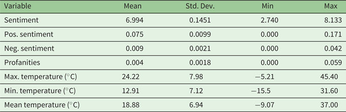
Descriptive statistics are presented in table 1. The sentiment index (Hedonometer) shows an average value of 6.99 with a standard deviation of 0.145. On average, 75 out of 1,000 words in the corpus are positive (scoring above 7), while 9.4 are negative (scoring below 3). Regarding the frequency of profanity, only 4.5 out of 1,000 words in the corpus belong to the dictionary we constructed to measure profane expressions. Summary statistics for temperature are also presented in table 1. The mean provincial daily maximum temperature in our sample is 24.2 $^{\circ }$C.
Descriptive statistics

Table 1 Long description
The table has four columns: Variable, Mean, Std. Dev., Min, Max. Row 1: Sentiment 6.994, 0.1451, 2.740, 8.133. Row 2: Pos. sentiment 0.075, 0.0099, 0.000, 0.171. Row 3: Neg. sentiment 0.009, 0.0021, 0.000, 0.042. Row 4: Profanities 0.004, 0.0018, 0.000, 0.059. Row 5: Max. temperature (degrees Celsius) 24.22, 7.98, -5.21, 45.40. Row 6: Min. temperature (degrees Celsius) 12.91, 7.12, -15.5, 31.60. Row 7: Mean temperature (degrees Celsius) 18.88, 6.94, -9.07, 37.00.
Notes: Number of observations is 35,309 corresponding to a combination of day and province (except for minimum and mean temperature which is 33,162 due to missing data). The sample spans the period from November 2017 to February 2022. Social media metrics correspond to all geo-tagged posts within Argentina during this time-frame. The maximum temperature corresponding to a province-day is equal to the average maximum temperature for every station in the corresponding province weighted by the population of the administrative district (departamento) of each station.
Finally, table A2 in the online appendix confirms that the weekly cycle of overall social media sentiment, as reported by Dodds et al. (Reference Dodds, Harris, Kloumann, Bliss and Danforth2011), is also present in our corpus. Tweets on Fridays, Saturdays, and Sundays display higher levels of happiness compared to the rest of the week. With varied intensities, weekly cycles can also be detected for positive sentiment, negative sentiment, and profanity.
4 Results
In this section we summarize our findings. Note that all the results are measured in standard deviations. In the figures, we also include the 95th per cent confidence interval for the central estimate.
4.1 Relationship between expressed sentiments and temperature
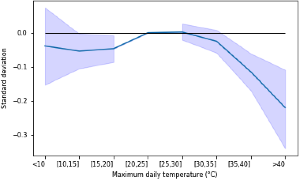
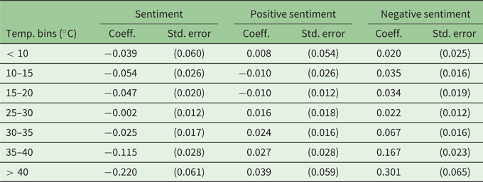
Figure 2 and the first columns in table 2 present the results for the first index of social media content, i.e., sentiments. The estimations indicate a negative association between extreme temperatures and overall sentiment. Low temperatures have a negative impact on well-being. More precisely, a statistically significant impact of approximately 0.05 standard deviations is estimated for temperature bins [10–15] and [15–20]. Conversely, a statistically significant impact is observed for temperatures exceeding 35 $^{\circ }$C, with the most substantial impact occurring for daily maximum temperatures surpassing 40
 $^{\circ }$C – resulting in an estimated impact on well-being exceeding 0.22 standard deviations. Consequently, extreme heat has a more pronounced effect on well-being than extreme cold, as reflected in social media sentiments. Notably, despite the wide confidence intervals associated with extremely high temperatures, the estimations point to statistically significant impacts.Footnote 22
Overall sentiment and maximum daily temperature, Notes: This figure plots the estimated coefficients for daily maximum temperature bins from empirical model (1) and reported in column 2 of table 1. The dependent variable is the standardized metrics of sentiment. The number of observations is 35,309, each corresponding to a unique day-province combination. Regressions include fixed effects for province, month, year, and day of the week. Coefficients represent mean differences with respect to expected values for the [20–25] $^\circ$C temperature bin. Standard errors are clustered by province. The shaded area corresponds to the 95th confidence intervals.

Figure 2 Long description
The x-axis label is “Maximum daily temperature (°C)”. The x-axis categories, from left to right, are “<10”, “[10,15]”, “[15,20]”, “[20,25]”, “[25,30]”, “[30,35]”, “[35,40]”, “>40”. The y-axis label is “Standard deviation”. The y-axis tick labels shown are 0.0, −0.1, −0.2 and −0.3. A single line is plotted across the temperature bins. The line is below 0.0 at “<10”, “[10,15]” and “[15,20]”. The line is at 0.0 at “[20,25]” and “[25,30]”. The line is below 0.0 at “[30,35]”, “[35,40]” and “>40”, with the lowest point at “>40”. A shaded band surrounds the line. The band is widest at “<10” and “>40” and narrower around the middle bins.
Sentiment and maximum daily temperature
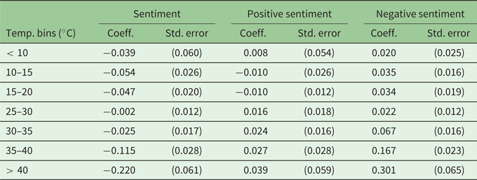
Table 2 Long description
The table has four columns: Temp. bins (degrees Celsius), Sentiment, Positive sentiment, Negative sentiment. Row 1: Temp. bins < 10, Sentiment Coeff. -0.039, Std. error 0.060; Positive sentiment Coeff. 0.008, Std. error 0.054; Negative sentiment Coeff. 0.020, Std. error 0.025. Row 2: Temp. bins 10–15, Sentiment Coeff. -0.054, Std. error 0.026; Positive sentiment Coeff. -0.010, Std. error 0.026; Negative sentiment Coeff. 0.035, Std. error 0.016. Row 3: Temp. bins 15–20, Sentiment Coeff. -0.047, Std. error 0.020; Positive sentiment Coeff. -0.010, Std. error 0.012; Negative sentiment Coeff. 0.034, Std. error 0.019. Row 4: Temp. bins 25–30, Sentiment Coeff. -0.002, Std. error 0.012; Positive sentiment Coeff. 0.016, Std. error 0.018; Negative sentiment Coeff. 0.022, Std. error 0.012. Row 5: Temp. bins 30–35, Sentiment Coeff. -0.025, Std. error 0.017; Positive sentiment Coeff. 0.024, Std. error 0.016; Negative sentiment Coeff. 0.067, Std. error 0.016. Row 6: Temp. bins 35–40, Sentiment Coeff. -0.115, Std. error 0.028; Positive sentiment Coeff. 0.027, Std. error 0.028; Negative sentiment Coeff. 0.167, Std. error 0.023. Row 7: Temp. bins > 40, Sentiment Coeff. -0.220, Std. error 0.061; Positive sentiment Coeff. 0.039, Std. error 0.059; Negative sentiment Coeff. 0.301, Std. error 0.065.
Notes: This table reports the estimated coefficients for daily maximum temperature bins from empirical model (1). The dependent variables are the standardized metrics of well-being (Hedonometer), positive sentiment, and negative sentiment, respectively. The number of observations is 35,309, each corresponding to a unique day-province combination. Regressions include fixed effects for province, month, year, and day of the week. Coefficients represent mean differences with respect to expected values for the [20–25] $^\circ$C temperature bin. Standard errors (in parentheses) are clustered by province.
Our findings regarding the impact of extreme temperatures on sentiment closely mirror those documented by Baylis (Reference Baylis2020) in the US context when temperatures are high. However, when temperatures are low, our results indicate a less substantial impact. Furthermore, it is noteworthy that the estimated impact of extreme positive temperatures bears similarity to the magnitude of the weekly cycle, as reported in column 2 of table A2 in the online appendix. These nuanced distinctions in the effects of extreme temperatures on sentiment underscore the importance of considering contextual factors and regional variations in the relationship between weather conditions and public sentiment.
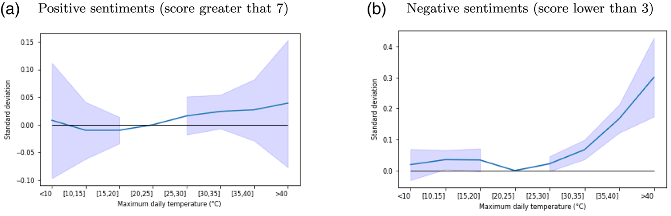
A more granular analysis of the impact of extreme temperatures on well-being is achieved by disaggregating the Hedonometer into positive and negative sentiments. This approach proves valuable as it allows for an important differentiation since, as mentioned above, having low negative feelings does not imply having high positive ones. Two distinct metrics are generated, indicating the frequency of positive or negative words as a fraction of the total number of words in the document. Figure 3 and table 2 present the estimated impact of extreme weather on these sentiment metrics. Notably, positive sentiment does not exhibit a significant response to temperature variations. The analysis of negative sentiment reveals a strong positive correlation with extreme temperatures. Specifically, temperatures above 40 $^\circ$C result in a significant increase of 0.301 standard deviations in the negative sentiment index. In contrast, extremely low temperatures (below 10
 $^\circ$C) do not elicit a statistically significant response in negative sentiment. This asymmetry between negative and positive sentiment responses highlights the unique impact of heat on negative emotions. Consequently, the overall effect of extremely high temperatures on sentiment is primarily driven by an increase in negative feelings during hot weather conditions.
Positive and negative sentiments and maximum daily temperature, (a) Positive sentiments (score greater that 7), (b) Negative sentiments (score lower than 3). Notes: This figure plots the estimated coefficients for daily maximum temperature bins from empirical model (1) and reported in columns 4 and 6 of table 2. The dependent variables are the standardized metrics positive sentiment (panel a), and negative sentiment (panel b). The number of observations is 35,309, each corresponding to a unique day-province combination. Regressions include fixed effects for province, month, year, and day of the week. Coefficients represent mean differences with respect to expected values for the [20–25] $^\circ$C temperature bin. Standard errors are clustered by province. The shaded area corresponds to the 95th confidence intervals.

Figure 3 Long description
The image A showing (a) Positive sentiments (score greater that 7). Horizontal axis label: Maximum daily temperature (degree Celsius). Temperature bins: less than 10, 10 to 15, 15 to 20, 20 to 25, 25 to 30, 30 to 35, 35 to 40, greater than 40. Vertical axis label: Standard deviation. Labeled ticks: negative 0.10, negative 0.05, 0.00, 0.05, 0.10, 0.15. A single solid line is plotted with a shaded band around parts of the line. Plotted line coordinate pairs are not shown with numeric point labels. The line is near 0.00 at less than 10, slightly below 0.00 at 10 to 15 and 15 to 20, near 0.00 at 20 to 25, above 0.00 at 25 to 30 and increases slightly from 30 to 35 through greater than 40. The image B showing (b) Negative sentiments (score lower than 3). Horizontal axis label: Maximum daily temperature (degree Celsius). Temperature bins: less than 10, 10 to 15, 15 to 20, 20 to 25, 25 to 30, 30 to 35, 35 to 40, greater than 40. Vertical axis label: Standard deviation. Labeled ticks: 0.0, 0.1, 0.2, 0.3, 0.4. A single solid line is plotted with a shaded band around parts of the line. Plotted line coordinate pairs are not shown with numeric point labels. The line is slightly above 0.0 at less than 10, around 0.03 to 0.04 at 10 to 15 and 15 to 20, near 0.0 at 20 to 25, above 0.0 at 25 to 30, rises at 30 to 35, rises further at 35 to 40 and reaches its highest level at greater than 40. Across the two graphs, the negative sentiments line rises more at higher temperature bins than the positive sentiments line.
4.2 Relationship between on-line aggression and temperature
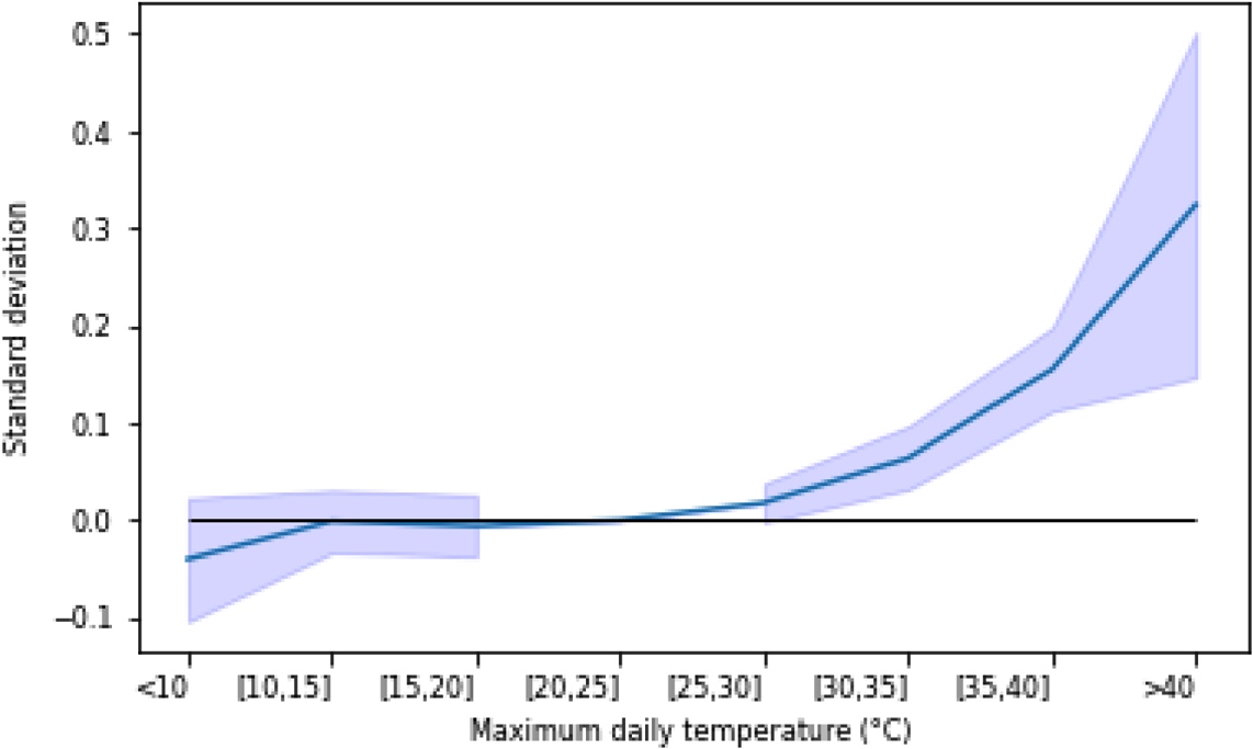
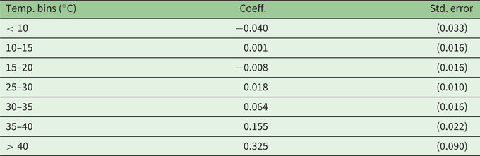
Regarding the association between extreme temperatures and aggression in social media, figure 4 and table 3 show that extreme temperatures cause a rise in expressions of profanity. There is a statistically significant association found in the case of high temperatures. A maximum temperature higher than 40 $^{\circ }$C causes an increase of 0.237 standard deviations in the frequency of expressions of profanities in social media relative to the omitted temperature bin.
Profanity frequency and maximum daily temperature. Notes: This figure plots the estimated coefficients for daily maximum temperature bins from empirical model (1) and reported in column 2 of table 3. The dependent variable is the standardized metrics of profanities. The number of observations is 35,309, each corresponding to a unique day-province combination. Regressions include fixed effects for province, month, year, and day of the week. Coefficients represent mean differences with respect to expected values for the [20–25] $^\circ$C temperature bin. Standard errors are clustered by province. The shaded area corresponds to the 95th confidence intervals.

Figure 4 Long description
The x-axis label is Maximum daily temperature (°C). The x-axis categories, from left to right, are <10, [10,15], [15,20], [20,25], [25,30], [30,35], [35,40], >40. The y-axis label is Standard deviation. The y-axis ranges from -0.1 to 0.5. A line is plotted across the temperature bins with a shaded band around it. The line values shown are: <10 at -0.040, [10,15] at 0.001, [15,20] at -0.008, [20,25] at 0.000, [25,30] at 0.018, [30,35] at 0.064, [35,40] at 0.155 and >40 at 0.325.
Profanity frequency and maximum daily temperature
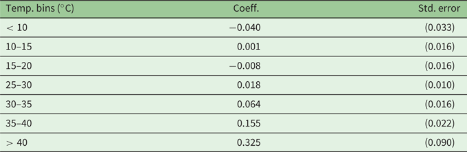
Table 3 Long description
The table has three columns: Temp. bins (°C), Coeff. and Std. error. Row 1: Temp. bins < 10, Coeff. -0.040, Std. error (0.033). Row 2: Temp. bins 10–15, Coeff. 0.001, Std. error (0.016). Row 3: Temp. bins 15–20, Coeff. -0.008, Std. error (0.016). Row 4: Temp. bins 25–30, Coeff. 0.018, Std. error (0.010). Row 5: Temp. bins 30–35, Coeff. 0.064, Std. error (0.016). Row 6: Temp. bins 35–40, Coeff. 0.155, Std. error (0.022). Row 7: Temp. bins > 40, Coeff. 0.325, Std. error (0.090).
Notes: This table reports the estimated coefficients for daily maximum temperature bins from empirical model (1). The dependent variable is standardized metrics of profanities. The number of observations is 35,309, each corresponding to a unique day-province combination. Regressions include fixed effects for province, month, year, and day of the week. Coefficients represent mean differences with respect to expected values for the [20–25] $^\circ$C temperature bin. Standard errors (in parentheses) are clustered by province.
Conversely, the impact of extremely cold temperatures (below 10 $^{\circ }$C) suggests a decrease in the frequency of profanity usage. A maximum temperature lower than 10
 $^\circ$C results in a decrement of 0.04 standard deviations in the frequency of profanity expressions in social media. It is noteworthy that the amplified incidence of negative profanities during extremely high temperatures is fourfold compared to the negative impact of very low temperatures on profanity occurrence. This divergence emphasizes the asymmetrical influence of temperature extremes on the expression of negative language in social media.
In summary, consistent with prevailing trends in the existing literature, we have documented that extreme temperatures affect people's sentiment. However, the precise shape of this relationship diverges from the conventional inverted U-shape reported by Baylis (Reference Baylis2020) for the US. Like the findings of Wang et al. (Reference Wang, Obradovich and Zheng2020) for China, the effect of extremely cold temperatures in our study is less pronounced. Notably, our results indicate that the influence of high temperatures is predominantly driven by an increase in negative sentiments rather than a decline in positive ones. Additionally, the relationship with profanities exhibits more of an upward curved shape, closely resembling the pattern observed in negative sentiments. This pattern reveals the complex relationship between temperature and various aspects of online expression. It indicates that environmental conditions affect different types of social media content in distinct ways.
4.3 Additional analysis
We conduct various complementary exercises to validate our findings and to provide a more detailed picture of the association between extreme temperatures and expressed sentiments in social media.
4.3.1 Alternative specifications of the empirical model
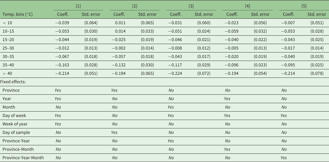
In this subsection we consider changes in the empirical model that address potential features of the data that might affect our results. First, allowing for a higher frequency measurement of seasonality, we substitute month fixed effect by week of year fixed effects. In an additional robustness test that contemplates high frequency variation in unconditional average sentiment, we substitute year, month and day of week fixed effects by day of sample fixed effects. In a complementary evaluation, we consider regional trends by introducing province-year fixed effects. Regional seasonality is addressed through a specification that incorporates province-month fixed effects. Finally, regional seasonality and regional trends are contemplated simultaneously by a model with province-year-month fixed effects.
The estimated parameters of these alternative empirical model specifications are reported in table 4. To a large extent, the previously reported results are verified in these complementary evaluations. In particular, in all cases, extreme heat is associated with a drop in the mean metric of expressed sentiment (Hedonometer). It is worth noting that, in each case, the magnitude of these effects is similar to that reported above (see column 2 of table 2).
Robustness: alternative specifications of the empirical model
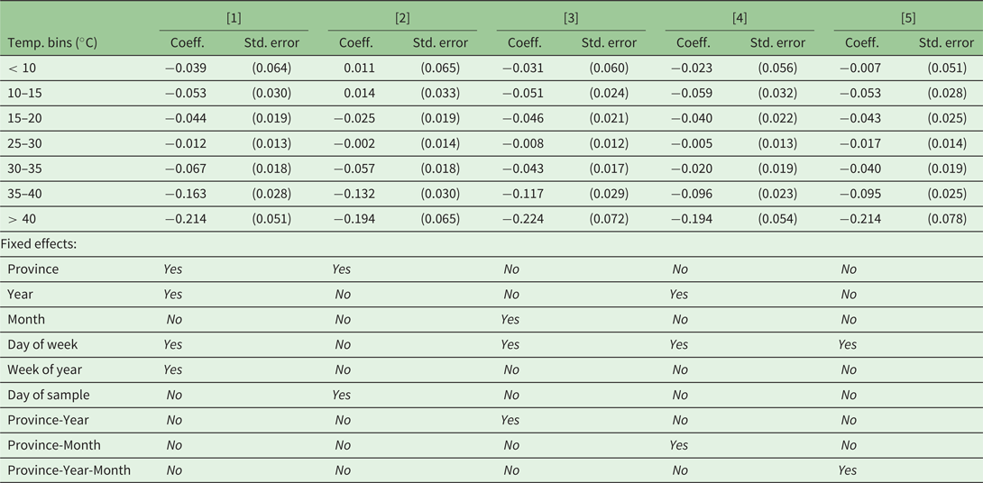
Table 4 Long description
The table has columns: Temp. bins (degrees Celsius), [1] Coeff., [1] Std. error, [2] Coeff., [2] Std. error, [3] Coeff., [3] Std. error, [4] Coeff., [4] Std. error, [5] Coeff., [5] Std. error. Row 1: < 10, -0.039, 0.064, 0.011, 0.065, -0.031, 0.060, -0.023, 0.056, -0.007, 0.051. Row 2: 10–15, -0.053, 0.030, 0.014, 0.033, -0.051, 0.024, -0.059, 0.032, -0.053, 0.028. Row 3: 15–20, -0.044, 0.019, -0.025, 0.019, -0.046, 0.021, -0.040, 0.022, -0.043, 0.025. Row 4: 25–30, -0.012, 0.013, -0.002, 0.014, -0.008, 0.012, -0.005, 0.013, -0.017, 0.014. Row 5: 30–35, -0.067, 0.018, -0.057, 0.018, -0.043, 0.017, -0.020, 0.019, -0.040, 0.016. Row 6: 35–40, -0.163, 0.028, -0.132, 0.030, -0.117, 0.029, -0.096, 0.023, -0.095, 0.025. Row 7: > 40, -0.214, 0.051, -0.194, 0.065, -0.224, 0.072, -0.194, 0.054, -0.214, 0.078. Fixed effects include Province, Year, Month, Day of week, Week of year, Day of sample, Province-Year, Province-Month, Province-Year-Month, with varying inclusion across models.
Notes: This table reports the estimated coefficients for daily maximum temperature bins with different sets of fixed effects. The dependent variable is standardized metrics sentiment (Hedonometer). The number of observations is 35,309, each corresponding to a unique day-province combination. Coefficients represent mean differences with respect to expected values for the [20–25] $^\circ$C temperature bin. Standard errors (in parentheses) are clustered by province.
4.3.2 Alternative specifications of the well-being metric
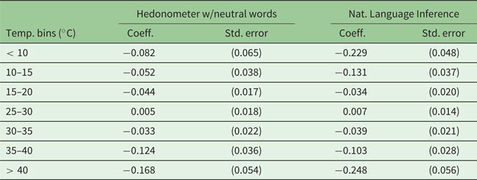
In this subsection we evaluate the association between extreme temperatures and sentiments in social media for alternative specifications of the well-being metric. First, we consider an alternative parametrization of the Hedonometer metric. More specifically, departing from the previous analysis, we evaluate the association for the case in which neutral words are part of the computation of the index. In addition, we consider a sentiment metric computed via large language model classification. Given the high computational cost of this method, the classifications were implemented for a subsample of the corpus.
The Hedonometer is a dictionary-based method in which the sentiment index equals the average tonality of selected words. The developers of the method have suggested that a more informative indicator can result if neutral words are disregarded (Dodds and Danforth, Reference Dodds and Danforth2010; Dodds et al, Reference Dodds, Harris, Kloumann, Bliss and Danforth2011). Following this suggestion, in the analysis above, words with intermediate rating (above 3 and below 7) were not part of the computation of the index. To check for the robustness of our results, we perform a complementary evaluation in which the Hedonometer is computed using the full dictionary of 10,000 words. The results are reported in the first columns of table 5. The results are very similar to the findings of our baseline model (column 2 of table 2), suggesting that our results are robust to changes in the specification of the Hedonometer.
Alternative well-being metrics

Table 5 Long description
The table has five columns: Temp. bins (°C), Hedonometer w/neutral words Coeff., Hedonometer w/neutral words Std. error, Nat. Language Inference Coeff., Nat. Language Inference Std. error. Row 1: < 10, -0.082, 0.065, -0.229, 0.048. Row 2: 10–15, -0.052, 0.038, -0.131, 0.037. Row 3: 15–20, -0.044, 0.017, -0.034, 0.020. Row 4: 25–30, 0.005, 0.018, 0.007, 0.014. Row 5: 30–35, -0.033, 0.022, -0.039, 0.021. Row 6: 35–40, -0.124, 0.036, -0.103, 0.028. Row 7: > 40, -0.168, 0.054, -0.248, 0.056.
Notes: This table reports the estimated coefficients for daily maximum temperature bins from empirical model (1). The dependent variables are the standardized metrics of well-being: Hedonometer with neutral words and NLI, respectively. The number of observations is 35,309, each corresponding to a unique day-province combination. Regressions include fixed effects for province, month, year, and day of the week. Coefficients represent mean differences with respect to expected values for the [20–25] $^\circ$C temperature bin. Standard errors (in parentheses) are clustered by province.
We also explore sentiment classification using large language models, specifically employing Natural Language Inference (NLI) techniques. Due to high computational costs, this approach was applied to a subsample of 8 million geo-tagged tweets, approximately 10 per cent of our full dataset. The NLI model was trained to determine if a given text (premise) is consistent with or contradicts a second text (hypothesis). In our application, the premise is the social media message we aim to classify, while the hypotheses are formed by combining the template “Este es un ejemplo de sentimiento...” with labels “positivo,” “negativo,” or “neutral.”Footnote 23 The model assigns probabilities indicating whether each hypothesis is implied or contradicted by the premise. We derive a classification score for each message by subtracting the probability assigned to the “negative” label from that of the “positive” label. The sentiment index for a given province and day is then calculated as the average score of messages from that location and period. This implementation utilized a fine-tuned ROBERTA model trained on a multilingual dataset of labeled sentence pairs, providing an advanced, context-aware approach to sentiment analysis.Footnote 24
The estimated coefficients for temperature bins, reported in the fourth column of table 5, reveal a negative association between extreme temperatures and expressed well-being. For extremely high temperatures, the estimated impact aligns closely with our previous findings using the Hedonometer dictionary. Interestingly, the impact of low temperatures on expressed sentiment is also negative, with a larger effect than that estimated using the Hedonometer. This difference in the low-temperature effect might be attributed to the smaller sample size used in the NLI analysis.
4.3.3 Characterizing channels
To generate a more detailed characterization of the link between temperature and expressed sentiments, we assess the importance of discussions surrounding frequent power outages during summer, or debates about high temperatures. To do this, we estimate equation (1) while excluding all tweets explicitly mentioning heat or power outages. Tweets associated with each of these topics are identified using dictionaries built following the same methodology used above to build the profanity dictionary. That is, given a set of seed words, we expand the list recursively incorporating similar words as indicated by word embeddings and subjective judgment.
In the case of the first topic, electricity provision, a more direct method would involve controlling for power outages. Regrettably, explicit control for power outages in our empirical model is not possible due to incomplete records across all locations in our sample. Ideally, we would require detailed data on the number of affected users per location on a daily basis throughout the year. However, among those few electricity companies that do publicly report this data, it is typically aggregated on a monthly rather than daily basis.
While the seasonal nature of power outages, with higher occurrences during summer, is partially captured by month-fixed effects, we supplement this with an alternative approach in which we exclude messages that are judged likely to refer to problems with electricity provision. For this task, we follow the same strategy used to generate the list of profanity words to create a list word indicative of discussions related to electricity provision. We start with 3 seed words: “electricidad”, “luz” and “corte”Footnote 25 The resulting dictionary includes 22 keywords and results in the exclusion of approximately 1 per cent of the posts.
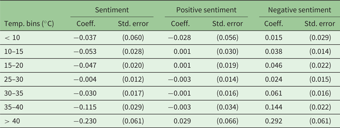
We recompute our sentiment indices excluding tweets containing any of those words. Table 6 reveals that eliminating tweets associated with electricity provision does not significantly alter the relationship between sentiment and temperature. While estimated coefficients and their statistical significance may experience slight changes, the direction and magnitude of the effects remain mostly unaltered.
Sentiment and maximum daily temperature excluding power outage mentions

Table 6 Long description
The table has seven columns: Temp. bins (degrees Celsius), Sentiment Coeff., Sentiment Std. error, Positive sentiment Coeff., Positive sentiment Std. error, Negative sentiment Coeff., Negative sentiment Std. error. Row 1: Temp. bins less than 10, Sentiment Coeff. -0.037, Sentiment Std. error 0.060, Positive sentiment Coeff. -0.028, Positive sentiment Std. error 0.056, Negative sentiment Coeff. 0.015, Negative sentiment Std. error 0.029. Row 2: Temp. bins 10–15, Sentiment Coeff. -0.053, Sentiment Std. error 0.028, Positive sentiment Coeff. 0.001, Positive sentiment Std. error 0.030, Negative sentiment Coeff. 0.038, Negative sentiment Std. error 0.014. Row 3: Temp. bins 15–20, Sentiment Coeff. -0.047, Sentiment Std. error 0.020, Positive sentiment Coeff. 0.001, Positive sentiment Std. error 0.019, Negative sentiment Coeff. 0.046, Negative sentiment Std. error 0.022. Row 4: Temp. bins 25–30, Sentiment Coeff. -0.004, Sentiment Std. error 0.012, Positive sentiment Coeff. -0.003, Positive sentiment Std. error 0.014, Negative sentiment Coeff. 0.024, Negative sentiment Std. error 0.015. Row 5: Temp. bins 30–35, Sentiment Coeff. -0.030, Sentiment Std. error 0.017, Positive sentiment Coeff. -0.001, Positive sentiment Std. error 0.016, Negative sentiment Coeff. 0.061, Negative sentiment Std. error 0.016. Row 6: Temp. bins 35–40, Sentiment Coeff. -0.115, Sentiment Std. error 0.029, Positive sentiment Coeff. -0.003, Positive sentiment Std. error 0.034, Negative sentiment Coeff. 0.144, Negative sentiment Std. error 0.022. Row 7: Temp. bins greater than 40, Sentiment Coeff. -0.230, Sentiment Std. error 0.061, Positive sentiment Coeff. 0.029, Positive sentiment Std. error 0.066, Negative sentiment Coeff. 0.292, Negative sentiment Std. error 0.061.
Notes: This table reports the estimated coefficients for temperature bins for empirical model (1) where the left-hand side variables are the standardized metric of sentiment (Hedonometer), the standardized metric of positive sentiment, and the standardized metric of negative sentiment, respectively. Regressions include fixed effects for province, month, year, and day of the week. Coefficients represent mean differences with respect to expected values for temperature bin [20–25] $^\circ$C. Standard errors (in parentheses) are clustered by province.
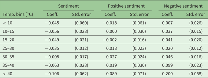
Regarding heat, as in Baylis (Reference Baylis2020), we try to exclude all tweets that capture the sentiments about heat and not changes in sentiments due to heat. We follow the same methodology as in the previous case using “calor” as a seed word. The resulting dictionary of 25 terms related to heat includes words such as: temperatura (temperature), caliente (hot), grados (degree Celsius). Excluded messages represent approximately 0.4 per cent of the original corpus messages. The results from this exercise are reported in table 7. In contrast to the case of electricity outages, the estimated coefficients are lower in magnitude. While they retain statistical significance, especially in the case of negative sentiment, these lower levels suggest that an important fraction of the negative impact of extreme heat on sentiments is channelled through messages that establish a direct link between weather conditions and expressed well-being.
Sentiment and maximum daily temperature excluding heat mentions
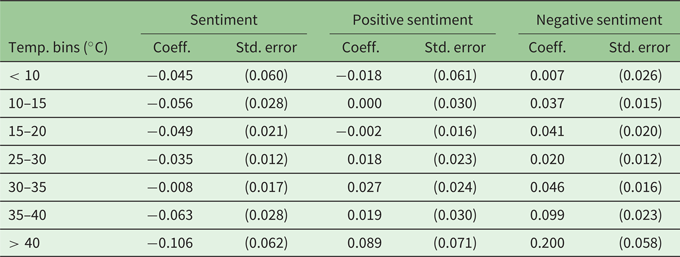
Table 7 Long description
The table has four columns: Temp. bins (degrees Celsius), Sentiment, Positive sentiment, Negative sentiment. Each sentiment category has two sub-columns: Coeff. and Std. error. Row 1: Temp. bins < 10, Sentiment Coeff. -0.045, Std. error 0.060; Positive sentiment Coeff. -0.018, Std. error 0.061; Negative sentiment Coeff. 0.007, Std. error 0.026. Row 2: Temp. bins 10–15, Sentiment Coeff. -0.056, Std. error 0.028; Positive sentiment Coeff. 0.000, Std. error 0.030; Negative sentiment Coeff. 0.037, Std. error 0.015. Row 3: Temp. bins 15–20, Sentiment Coeff. -0.049, Std. error 0.021; Positive sentiment Coeff. -0.002, Std. error 0.016; Negative sentiment Coeff. 0.041, Std. error 0.020. Row 4: Temp. bins 25–30, Sentiment Coeff. -0.035, Std. error 0.012; Positive sentiment Coeff. 0.018, Std. error 0.023; Negative sentiment Coeff. 0.020, Std. error 0.012. Row 5: Temp. bins 30–35, Sentiment Coeff. -0.008, Std. error 0.017; Positive sentiment Coeff. 0.027, Std. error 0.024; Negative sentiment Coeff. 0.046, Std. error 0.016. Row 6: Temp. bins 35–40, Sentiment Coeff. -0.063, Std. error 0.028; Positive sentiment Coeff. 0.019, Std. error 0.030; Negative sentiment Coeff. 0.099, Std. error 0.023. Row 7: Temp. bins > 40, Sentiment Coeff. -0.106, Std. error 0.062; Positive sentiment Coeff. 0.089, Std. error 0.071; Negative sentiment Coeff. 0.200, Std. error 0.058.
Notes: This table reports the estimated coefficients for temperature bins for empirical model (1) where the left-hand side variables are the standardized metric of sentiment (Hedonometer), the standardized metric of positive sentiment, and the standardized metric of negative sentiment, respectively. Regressions include fixed effects for province, month, year, and day of the week. Coefficients represent mean differences with respect to expected values for temperature bin [20–25] $^\circ$C. Standard errors (in parentheses) are clustered by province.
4.3.4 Alternative corpus
In our analysis, we primarily used geo-tagged tweets to compute local climate-specific indices. However, recognizing potential selection biases in this approach, we evaluated the robustness of our results using an alternative strategy. This second method identifies a location based on the user's self-reported information in their profile, following the procedure used in Aromí and Llada (Reference Aromí and Llada2023) for developing a macroeconomic indicator from social media content. We identified Argentine users by inspecting a large volume of tweets retrieved through the “sample” X-Twitter API endpoint, including users whose profiles contained the (lower-cased) term “argentina” From this database, we collected tweets from users reporting locations matching each province. This alternative dataset covers Argentine provinces from 2015 to 2021.
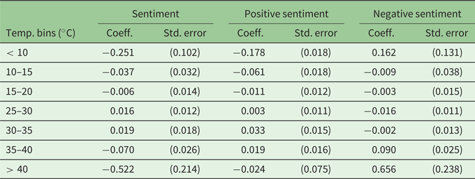
Consequently, we gather data from 3 million users. For each day and province, the corresponding tweets are combined to form a document which, in the subsequent stage, undergoes processing to generate daily provincial indicators. The comprehensive database encompasses 282 million tweets, presenting a sample 3.5 times more extensive than the geo-tagged dataset. Table 8 replicates the analysis of the correlation between temperature and sentiments. Estimations underscore the robustness of our findings regarding the impact of heat on overall sentiment, even when employing an alternative strategy to construct province-specific indices of social media content. On the other hand, we now observe a significant negative effect of colder temperatures on positive sentiments. Beyond these discrepancies, these complementary results suggest that there are multiple useful strategies that can be used to generate geo-located indicators of social media content. Both geo-tagged messages and user profile data result in consistent findings regarding the impact of extreme temperature on well-being.
Sentiment and maximum daily temperature with alternative X-Twitter corpus

Table 8 Long description
The table has four columns: Temp. bins (degrees Celsius), Sentiment, Positive sentiment, Negative sentiment. Each sentiment category has two sub-columns: Coeff. and Std. error. Row 1: Temp. bins < 10, Sentiment Coeff. -0.251, Std. error 0.102; Positive sentiment Coeff. -0.178, Std. error 0.018; Negative sentiment Coeff. 0.162, Std. error 0.131. Row 2: Temp. bins 10–15, Sentiment Coeff. -0.037, Std. error 0.032; Positive sentiment Coeff. -0.061, Std. error 0.018; Negative sentiment Coeff. -0.009, Std. error 0.038. Row 3: Temp. bins 15–20, Sentiment Coeff. -0.006, Std. error 0.014; Positive sentiment Coeff. -0.011, Std. error 0.012; Negative sentiment Coeff. -0.003, Std. error 0.015. Row 4: Temp. bins 25–30, Sentiment Coeff. 0.016, Std. error 0.012; Positive sentiment Coeff. 0.003, Std. error 0.011; Negative sentiment Coeff. 0.001, Std. error 0.011. Row 5: Temp. bins 30–35, Sentiment Coeff. 0.019, Std. error 0.018; Positive sentiment Coeff. 0.033, Std. error 0.015; Negative sentiment Coeff. -0.002, Std. error 0.013. Row 6: Temp. bins 35–40, Sentiment Coeff. -0.070, Std. error 0.026; Positive sentiment Coeff. 0.019, Std. error 0.016; Negative sentiment Coeff. 0.090, Std. error 0.025. Row 7: Temp. bins > 40, Sentiment Coeff. -0.522, Std. error 0.214; Positive sentiment Coeff. -0.024, Std. error 0.075; Negative sentiment Coeff. 0.656, Std. error 0.238.
Notes: This table reports the estimated coefficients for temperature bins for empirical model (1) where the left-hand side variables are the standardized metric of sentiment (Hedonometer), the standardized metric of positive sentiment, and the standardized metric of negative sentiment, respectively. Regressions include fixed effects for province, month, year, and day of the week. Coefficients represent mean differences with respect to expected values for temperature bin [20–25] $^\circ$C. Standard errors (in parentheses) are clustered by province.
5 Conclusions
In this paper, we analyze approximately 80 million geo-tagged tweets from Argentina spanning the period 2017–2022 to investigate the influence of temperature on various indices related to human well-being. Our study includes the application of the Hedonometer Index to study overall sentiment, dissecting positive and negative sentiments separately, and assessing social media aggressive behavior through the frequency of profanities.
Our research has revealed a strong negative causal relationship between extreme heat and overall sentiment expressed on social media. However, in the case of extreme cold temperatures, we find weaker evidence of a negative impact on sentiment. Consequently, in the Argentinean context, our data does not support the existence of a clear inverted-U shaped curve between temperature and social media sentiment. In this sense, our findings align more closely with those reported by Wang et al. (Reference Wang, Obradovich and Zheng2020) in China and Baylis (Reference Baylis2020) for the Philippines and South Africa. Additionally, our results indicate that, while heat strongly influences negative sentiments, it has no significant effect on positive ones. Consequently, the overall impact of extremely high temperatures on sentiment is predominantly driven by heightened negative feelings during hot conditions. Furthermore, the outcome for our profanity index exhibits a similar pattern to that observed for negative sentiments.
The relationship between temperature and online sentiment or aggression is of critical importance, as weather significantly affects self-reported happiness. As climate change progresses, the vast amount of data from social media platforms could become a valuable tool for researchers and policymakers to track its ongoing effects on human well-being. García-Witulski et al. (Reference García-Witulski, Rabassa, Grand and Rozenberg2019) have already demonstrated that in Argentina, higher temperatures correlate with increased mortality rates. This underscores the vital need for the health sector to prepare adequately for the challenges posed by continuing climate change.
Furthermore, social media aggression might trigger physical violence. Numerous studies have highlighted the connection between online aggression and real-world violence (Simister and Cooper, Reference Simister and Cooper2005; Peterson and Densley, Reference Peterson and Densley2017; Sanz-Barbero et al., Reference Sanz-Barbero, Linares, Vives-Cases, González, López-Ossorio and Díaz2018; Xu et al., Reference Xu, Xiong, Abramson, Li and Guo2021), with at least one study demonstrating the causal impact of online hostility on physical violence (Du, Reference Du2023). This underscores the importance of unraveling the intricate relationship between temperature, sentiments, and social media aggression for a comprehensive understanding of the societal implications of climate change. If the link between virtual and physical violence is confirmed, monitoring social media will become even more essential, especially considering that police work intensity appears to decrease with rising temperatures. For instance, research by Heilmann et al. (Reference Heilmann, Kahn and Tang2021) shows that police patrols in Los Angeles decline on extremely hot days. Additionally, Obradovich et al. (Reference Obradovich, Tingley and Rahwan2018) find that high temperatures reduce police productivity. Therefore, our findings are crucial for informing adaptation strategies, preparing funding, and allocating personnel for violence helplines and security agencies to ensure resilience during periods of extreme heat. Merely preparing the health sector and issuing heat warnings will not be sufficient.
Our study offers valuable insights, but it is important to recognize its limitations. Firstly, sentiment expressions on X-Twitter may imperfectly measure emotional states, as individuals vary in how they express feelings, and some may disguise their true emotions. In essence, tweets represent expressions of sentiments, which may not perfectly align with the actual sentiments.Footnote 26 Additionally, we must note that we perform the analysis for a limited set of sentiment measurement methodologies. Sentiment analysis remains an active field in NLP. As a result, novel techniques might result in reassessments of the findings.
Secondly, X-Twitter users constitute only a fraction of the entire population, introducing a demographic bias. Twitter statistics for Argentina indicate that as of January 2021, 61.2 per cent of users are male, and data from July 2020 reveals that only 4 per cent of urban dwellers with basic education have accounts, while 33 per cent of those with tertiary or higher education levels are users. The age distribution is notably skewed, with 27 per cent of Argentinian centennials (under 25 years old) using the platform, compared to slightly over 5 per cent for individuals above 55 years old.Footnote 27 Consequently, older individuals and those with lower education levels, who might be more vulnerable to temperature impacts, are under-represented.Footnote 28 Thus, our estimate serves as a conservative approximation of the overall impact of temperature on sentiments.
Thirdly, our study faces limitations concerning climatological and environmental conditions. Some studies suggest that air pollution is linked to increased violence (e.g., Burkhardt et al., Reference Burkhardt, Bayham, Wilson, Berman, O'Dell, Ford, Fischer and Pierce2020; Kuo and Putra, Reference Kuo and Putra2021; Heilmann et al., Reference Heilmann, Kahn and Tang2021). Unfortunately, we lack data on air pollution to incorporate this dimension into our analysis. Furthermore, potential biases in the experienced temperature might arise from how our climate variables are constructed – using a weighted average from the meteorological stations closest to the city where the tweet user is located. Also, we assume uniform temperature exposure for all individuals within each province, neglecting factors such as working conditions (e.g., shade or sun exposure) or access to amenities like air conditioning. However, these kinds of measurement errors cannot be overcome with the available data.
Finally, future work to assess insights on social media sentiments for different sociodemographic groups would be important, as their responses to temperature extremes may diverge. For example, Wang et al. (Reference Wang, Obradovich and Zheng2020) report a heterogeneous impact of extreme temperature by gender. However, tackling this task is challenging, given the constraints in accurately identifying users’ characteristics, such as gender, age, or income levels, within X-Twitter posts. Another limitation is that access to X-Twitter data has become more restricted since the change in management. This development is expected to significantly impact future research possibilities and the replicability of studies that rely on X-Twitter data.
While the precise transmission mechanisms from temperature to sentiments or social media aggression remain unknown, our data unequivocally demonstrate a connection between higher-than-comfortable temperatures and negative sentiment, as well as social media aggression. This serves as an alarming signal considering anticipated future temperature increases in the country. As highlighted by several scholars, adaptation may not offer a viable solution to mitigate psychological stress or crime associated with temperature (e.g., Burke et al., Reference Burke, González, Baylis, Heft-Neal, Baysan, Basu and Hsiang2018; Baysan et al., Reference Baysan, Burke, González, Hsiang and Miguel2019). Wang et al. (Reference Wang, Obradovich and Zheng2020) specifically assert that even if China were to achieve economic parity with the US, resulting in increased adaptation capacity (e.g., more air conditioning appliances), the likelihood of decreased heat stress, as expressed in social media sentiments, remains low. Consequently, effective mitigation strategies are imperative to address the challenges posed by climate change.
Supplementary material
The supplementary material for this article can be found at https://doi.org/10.1017/S1355770X24000342
Acknowledgements
We express our gratitude for the valuable feedback received from Holly Krambech and Sahiti Sarva, as well as from the participants in the Heatwaves Collaborative Proposal Workshop, particularly Calvin Kwon, Gabriel Stefanini Vicente, Priyank Hirani, Aparna Keshaviah, Katie McWilliams, Alex Chunet, and David Rogers. Additionally, we appreciate the comments provided by Nancy Lozano Gracía, Richard Damania, Guadalupe Rojo, and participants of the BBL Workshop at the Buenos Aires WBG country office. We also gained valuable insights at the Economics Department Seminar at Universidad de San Andrés, Argentina. Access to Twitter data was possible through the Development Data Partnership (Project 324 “Well being and temperature in Argentina”).
Competing interests
The authors declare none.