1 Introduction
Leading-edge noise is a common and important source of noise generated by aeroengines when the wakes from forward rotor rows interact with rearward stator rows (Peake & Parry Reference Peake and Parry2012). Noise generated in this way can be reduced by altering the geometry of the blades, such as increasing blade thickness (Olsen & Wagner Reference Olsen and Wagner1982), varying mean loading (Mish & Devenport Reference Mish and Devenport2006a ,Reference Mish and Devenport b ), leading-edge radius (Ayton & Chaitanya Reference Ayton and Chaitanya2017) or a combination of these (Glegg & Devenport Reference Glegg and Devenport2017) however within the confines of an aeroengine some adaptations are not always practical. Therefore it is important to develop different alterations to the blades which will reduce noise but are appropriate for use within an aeroengine.
A popular adaptation to reduce leading-edge noise is to alter the spanwise straight leading edge of a blade to be serrated, which is inspired by the leading edges of owls’ wings (Graham Reference Graham1934; Lilley Reference Lilley1998) (albeit for the owl this likely yields and aerodynamic improvement rather than an acoustic improvement). A single-frequency serration is the most common adaptation investigated numerically (Clair et al. Reference Clair, Polacsek, Le Garrec, Reboul, Gruber and Joseph2013; Lau, Haeri & Kim Reference Lau, Haeri and Kim2013; Kim, Haeri & Joseph Reference Kim, Haeri and Joseph2016), experimentally (Hansen, Kelso & Doolan Reference Hansen, Kelso and Doolan2012; Narayanan et al. Reference Narayanan, Chaitanya, Haeri, Joseph, Kim and Polacsek2015; Biedermann et al. Reference Biedermann, Chong, Kameier and Paschereit2017; Chaitanya et al. Reference Chaitanya, Joseph, Narayanan, Vanderwel, Turner, Kim and Ganapathisubramani2017) and analytically (Huang Reference Huang2017; Lyu & Azarpeyvand Reference Lyu and Azarpeyvand2017; Ayton & Kim Reference Ayton and Kim2018). Whilst analytical solutions use very simplified models of convective gusts interacting with semi-infinite flat plates with leading-edge serrations, they can highlight key noise-reduction mechanisms that can only be speculated on from experimental and numerical results.
The single-frequency sawtooth serration (Hersh, Soderman & Hayden Reference Hersh, Soderman and Hayden1974) is believed to be effective in reducing leading-edge noise due to a destructive interference of scattered acoustics in the far field (Narayanan et al. Reference Narayanan, Chaitanya, Haeri, Joseph, Kim and Polacsek2015; Chaitanya et al. Reference Chaitanya, Joseph, Narayanan, Vanderwel, Turner, Kim and Ganapathisubramani2017; Lyu & Azarpeyvand Reference Lyu and Azarpeyvand2017), but recent analytical work has indicated a redistribution of acoustic energy from cuton modes to cutoff modes with increasing serration tip-to-root heights can also be important for overall noise reduction (Ayton & Kim Reference Ayton and Kim2018). With this understood the task is now to determine if different leading-edge geometries can result in better noise reductions through either an increased destructive interference, or greater ability to redistribute energy to the cutoff modes.
Current different designs include single-frequency sinusoidal leading edges (Mathews & Peake Reference Mathews and Peake2015; Kim et al. Reference Kim, Haeri and Joseph2016), double-frequency sinusoidal edges (Chaitanya et al. Reference Chaitanya, Joseph, Narayanan and Kim2018b ) and slitted profiles (Chaitanya et al. Reference Chaitanya, Narayanan, Joseph and Kim2016; Chaitanya & Joseph Reference Chaitanya and Joseph2018) and leading-edge hook structures (Geyer et al. Reference Geyer, Wasala, Cater, Norris and Sarradj2016). Experimentally it has been seen that different designs perform optimally in different flow situations (Chaitanya et al. Reference Chaitanya, Narayanan, Joseph and Kim2016; Chaitanya, Joseph & Ayton Reference Chaitanya, Joseph and Ayton2018a ). Since each design could be optimal in a different flow regime it is hard from purely experimental studies to conclusively determine which design is best overall. An analytic solution is valuable for understanding this; once the scattered acoustic field for an arbitrary leading-edge geometry has been determined, one can find the noise reductions predicted over a continuous range of flow parameters quickly without the need for repeated experiments or numerical simulations.
This paper therefore presents an analytic solution for the noise generated by a convective gust interacting with a semi-infinite flat plate with an arbitrary single-valued piecewise linear leading edge. To do so, we generalise the method used in Ayton & Kim (Reference Ayton and Kim2018) (adapted from the method used by Envia Reference Envia1988), which considers specifically the case of a single-frequency sawtooth serration, to a more general leading-edge geometry. This previous method utilises a tailored orthogonal expansion in the spanwise coordinate (i.e. not simply a Fourier series) that permits fully analytical progress through separation of variables and the Wiener–Hopf technique. Here we too shall tailor an expansion in the spanwise coordinate to the specific leading-edge geometry that will enable us to produce a fully analytic solution. This approach for an arbitrary piecewise linear serration geometry has been successfully used by Ayton (Reference Ayton2018) to analytically predict trailing-edge noise (the scattering of boundary-layer pressure fluctuations by the trailing edge of a plate).
We shall compare the analytic results against experimental measurements for five different leading-edge serration geometries. The experimental set-up uses a finite flat plate with a tripped boundary layer interacting with a straight trailing edge, therefore acoustic measurements are contaminated by trailing-edge self-noise. To account for this in the analytical model we add to the serrated leading-edge solution a simple analytical description of trailing-edge noise as developed by Amiet (Reference Amiet1976). Backscattering (of the leading-edge field by the trailing edge, or the trailing-edge field by the leading edge), as discussed by Roger & Moreau (Reference Roger and Moreau2005), Moreau & Roger (Reference Moreau and Roger2009), is not accounted for therefore we are able to treat each edge independently in this manner. This combined analytic and experimental study will enable us to validate the mathematical approach which can then be used to understand the key mechanisms for noise reduction due to a spanwise variable leading-edge geometry.
In addition to the simplicity of the solutions, a key benefit of these analytic results for the leading-edge field is that they permit a higher range of frequencies to be considered for leading-edge noise than experimental measurements (which are compounded by self-noise at high frequencies due to the finite trailing edge). It is important to have a clear understanding of the pure leading-edge noise as trailing-edge noise-reduction designs are also being investigated; porous and/or elastic trailing edges (Jaworski & Peake Reference Jaworski and Peake2013; Geyer & Sarradj Reference Geyer and Sarradj2014; Ayton Reference Ayton2016), serrated trailing edges (Lyu, Azarpeyvand & Sinayoko Reference Lyu, Azarpeyvand and Sinayoko2016; Oerlemans Reference Oerlemans2016), finlets (Clark et al. Reference Clark, Daly, Devenport, Alexander, Peake, Jaworski and Glegg2016) and trailing-edge brushes (Herr Reference Herr2006). These trailing-edge adaptations would reduce not only trailing-edge self-noise but also any rescattering of leading-edge noise (Huang Reference Huang2017), therefore an optimally quiet aerofoil would possess both a leading-edge adaptation and a trailing-edge adaptation. Whilst it is beyond the scope of this paper to consider the possible effects of both leading- and trailing-edge adaptations, we bear in mind that for an optimal design, any noise attributed to the trailing edge would also be significantly reduced from that predicted for a straight trailing edge and thus the leading-edge noise could become important over a wider range of frequencies than those for a plate with straight leading and trailing edges.
The layout of this paper is as follows. In § 2 we present the formulation of the mathematical problem for leading-edge noise generated by a semi-infinite flat plate with varying leading-edge geometry in the spanwise direction, which is similar to the formulation in Ayton & Kim (Reference Ayton and Kim2018). In § 3 we obtain the general analytic solution for an arbitrary periodic piecewise linear leading-edge geometry. In § 4 we discuss the experimental set-up, with § 4.5 discussing the effect of trailing-edge self-noise. In § 5 we present results for the far-field noise due to different leading-edge geometries and compare to the experimental results. Section 6 contains our conclusions.
2 Formulation of the problem
We consider the interaction of a convective unsteady gust in uniform flow of Mach number
 $M$
over a semi-infinite flat plate with a spanwise periodic leading edge. The plate lies in the region
 $x>\tilde{c}F(z)$
,
 $y=0$
, with
 $x$
denoting the streamwise direction,
 $y$
the normal direction and
 $\tilde{c}F(z)$
the periodic leading edge as a function of spanwise direction,
 $z$
. We non-dimensionalise lengths by the wavelength of the serration, velocities by the far upstream steady velocity and pressures by the far upstream density and velocity. We further normalise
 $F(z)$
for each geometry such that
 $\max _{z}F(z)-\min _{z}F(z)=1/2$
. This ensures definitions are aligned with Ayton & Kim (Reference Ayton and Kim2018) where such a normalisation was chosen so that sawtooth edges have unit derivatives,
 $|F^{\prime }(z)|=1$
. The parameter
 $\tilde{c}$
therefore permits a variable ‘tip-to-root’ ratio, i.e. varies the sharpness of the serration.
Since
 $F(z)$
is periodic we simplify the problem to considering a single wavelength of the leading-edge geometry, restricting to the spanwise region
 $0\leqslant z\leqslant 1$
. We impose quasi-periodic boundary conditions across
 $z=0,1$
. We restrict the leading-edge geometry such that
 $F(z)$
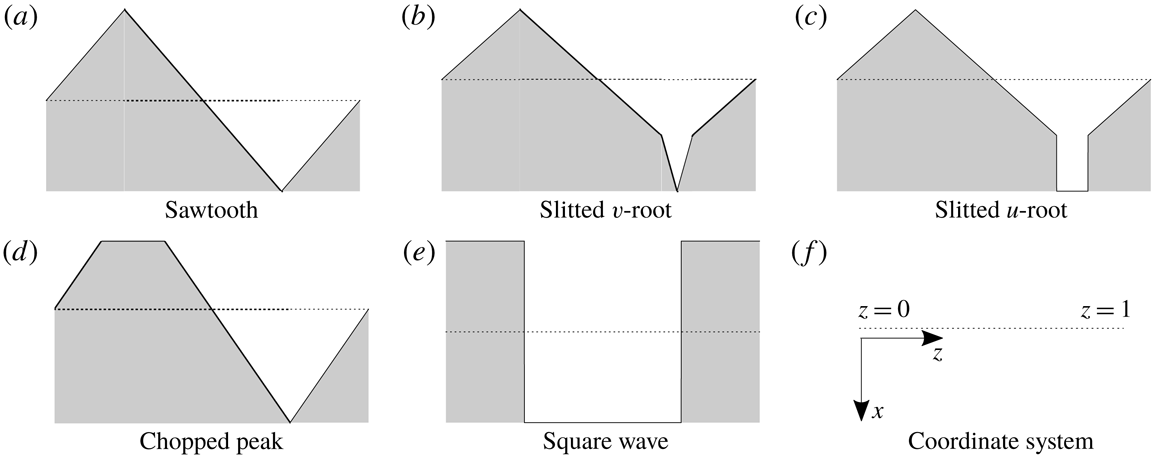
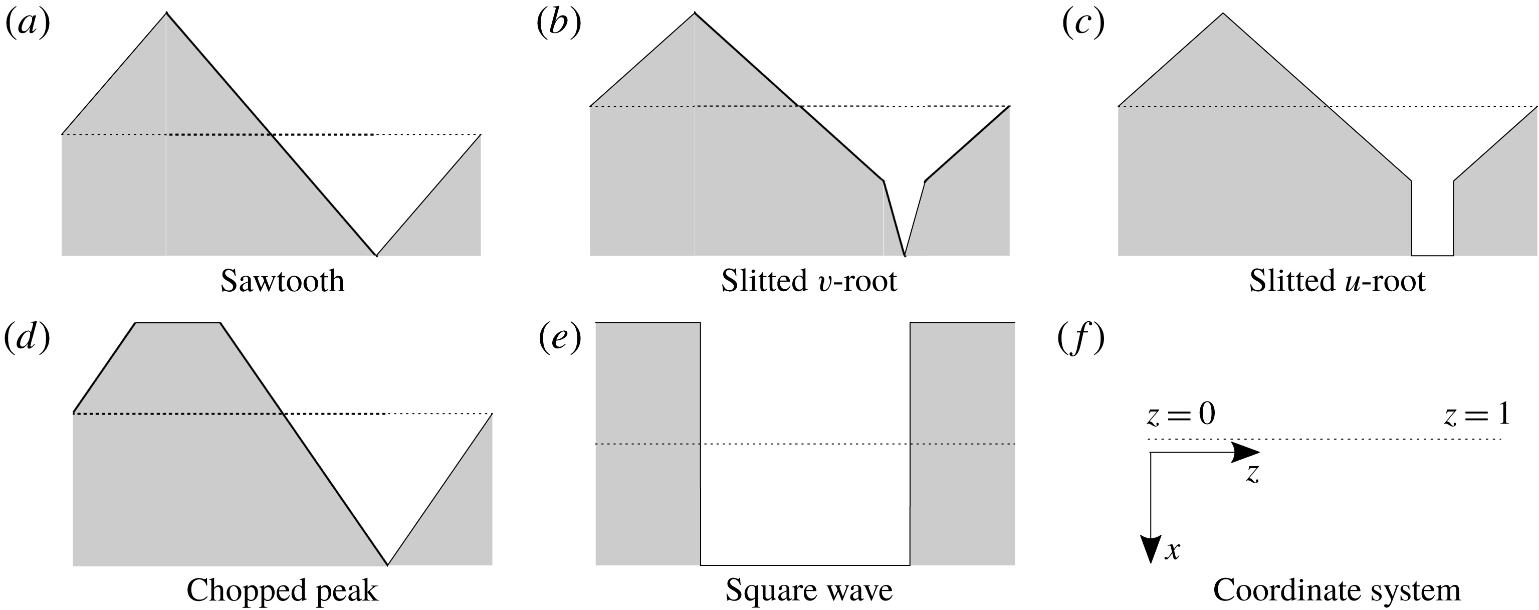
is a single-valued piecewise linear function, therefore we can investigate the most commonly used geometries such as the sawtooth serration and slitted root serration easily. Specifically in this paper we consider the five leading-edge geometries as depicted in figure 1 inspired by Chaitanya et al. (Reference Chaitanya, Narayanan, Joseph and Kim2016), although the results are applicable to any piecewise linear geometry (including piecewise linear approximations of any continuous periodic leading edge geometry such as a sinusoid), and dual-frequency serrations. Note in all geometry cases, the
 $z=0,1$
boundaries of the periodic function are chosen to be away from any region of discontinuity of the leading edge. This ensures the solution captures any influence of the discontinuities.
Leading-edge geometries,
 $x=F(z)$
. The shaded area depicts the rigid plate and the dashed line is along
 $x=0$
. Flow approaches the plate from the negative
 $x$
direction.
The unsteady gust incident from far upstream takes the form
 $$\begin{eqnarray}\boldsymbol{v}_{g}=\boldsymbol{A}\text{e}^{\text{i}k_{1}x+\text{i}k_{2}y+\text{i}k_{3}z-\text{i}\unicode[STIX]{x1D714}t},\end{eqnarray}$$
where the amplitude,
 $\boldsymbol{A}=(A_{1},A_{2},A_{3})^{\text{T}}$
, is constant. For simplicity we take
 $\boldsymbol{A}=(0,1,0)$
. As done for the specific sawtooth serration case in Ayton & Kim (Reference Ayton and Kim2018) we decompose the total unsteady flow field into a convective gust part and an acoustic response part,
 $\boldsymbol{v}=\boldsymbol{v}_{g}+\boldsymbol{v}_{a}$
, and write the response as
 $\boldsymbol{v}_{a}=\unicode[STIX]{x1D735}\unicode[STIX]{x1D719}$
. We suppose
 $\unicode[STIX]{x1D719}$
is harmonic in time
 ${\sim}\text{e}^{-\text{i}\unicode[STIX]{x1D714}t}$
therefore spatially satisfies the convective Helmholtz equation,
 $$\begin{eqnarray}\unicode[STIX]{x1D6FD}^{2}\frac{\unicode[STIX]{x2202}^{2}\unicode[STIX]{x1D719}}{\unicode[STIX]{x2202}x^{2}}+\frac{\unicode[STIX]{x2202}^{2}\unicode[STIX]{x1D719}}{\unicode[STIX]{x2202}y^{2}}+\frac{\unicode[STIX]{x2202}^{2}\unicode[STIX]{x1D719}}{\unicode[STIX]{x2202}z^{2}}+2\text{i}kM\frac{\unicode[STIX]{x2202}\unicode[STIX]{x1D719}}{\unicode[STIX]{x2202}x}+k^{2}\unicode[STIX]{x1D719}=0,\end{eqnarray}$$
where
 $\unicode[STIX]{x1D6FD}^{2}=1-M^{2}$
and
 $k=\unicode[STIX]{x1D714}/c_{0}$
with
 $c_{0}$
the speed of sound of the background steady flow. Since the gust convects with the background flow, we require
 $k=k_{1}M$
. The zero normal velocity boundary condition on the aerofoil surface requires
 $$\begin{eqnarray}\left.\frac{\unicode[STIX]{x2202}\unicode[STIX]{x1D719}}{\unicode[STIX]{x2202}y}\right|_{y=0}=-\text{e}^{\text{i}k_{1}x+\text{i}k_{3}z}\quad x>\tilde{c}F(z).\end{eqnarray}$$
We also impose continuity of the potential upstream
 $$\begin{eqnarray}\unicode[STIX]{x0394}\unicode[STIX]{x1D719}|_{y=0}=0\quad x<\tilde{c}F(z)\end{eqnarray}$$
and quasi-periodic conditions across
 $z=0,1$
,
 $$\begin{eqnarray}\unicode[STIX]{x1D719}|_{z=1}=\unicode[STIX]{x1D719}|_{z=0}\text{e}^{\text{i}k_{3}},\quad \left.\frac{\unicode[STIX]{x2202}\unicode[STIX]{x1D719}}{\unicode[STIX]{x2202}z}\right|_{z=1}=\left.\frac{\unicode[STIX]{x2202}\unicode[STIX]{x1D719}}{\unicode[STIX]{x2202}z}\right|_{z=0}\text{e}^{\text{i}k_{3}}.\end{eqnarray}$$
To simplify the governing equation, (2.2), we apply a convective transform,
 $$\begin{eqnarray}h=\unicode[STIX]{x1D719}(x,y,z)\text{e}^{\text{i}k_{1}M^{2}x/\unicode[STIX]{x1D6FD}^{2}},\end{eqnarray}$$
to eliminate the convective terms. The resulting governing equation and boundary conditions for
 $h(x,y,z)$
are
 $$\begin{eqnarray}\displaystyle & \displaystyle \unicode[STIX]{x1D6FD}^{2}\frac{\unicode[STIX]{x2202}^{2}h}{\unicode[STIX]{x2202}x^{2}}+\frac{\unicode[STIX]{x2202}^{2}h}{\unicode[STIX]{x2202}y^{2}}+\frac{\unicode[STIX]{x2202}^{2}h}{\unicode[STIX]{x2202}z^{2}}+\left(\frac{k_{1}M}{\unicode[STIX]{x1D6FD}}\right)^{2}h=0, & \displaystyle\end{eqnarray}$$
 $$\begin{eqnarray}\displaystyle & \displaystyle \left.\frac{\unicode[STIX]{x2202}h}{\unicode[STIX]{x2202}y}\right|_{y=0}=-\text{e}^{\text{i}(k_{1}/\unicode[STIX]{x1D6FD}^{2})x+\text{i}k_{3}z}\quad x>\tilde{c}F(z), & \displaystyle\end{eqnarray}$$
 $$\begin{eqnarray}\displaystyle & \unicode[STIX]{x0394}h|_{y=0}=0\quad x<\tilde{c}F(z), & \displaystyle\end{eqnarray}$$
 $$\begin{eqnarray}h|_{z=1}=h|_{z=0}\text{e}^{\text{i}k_{3}},\quad \left.\frac{\unicode[STIX]{x2202}h}{\unicode[STIX]{x2202}z}\right|_{z=1}=\left.\frac{\unicode[STIX]{x2202}h}{\unicode[STIX]{x2202}z}\right|_{z=0}\text{e}^{\text{i}k_{3}}.\end{eqnarray}$$
This system of equations, (2.5), is identical to that in Ayton & Kim (Reference Ayton and Kim2018), however, now, as we are considering a much broader range of leading-edge geometries, we must employ a different system of variable changes in order to solve it. We choose the following variables, as used by Roger, Schram & De Santana (Reference Roger, Schram and De Santana2013);
 $$\begin{eqnarray}\displaystyle & \displaystyle \unicode[STIX]{x1D709}=\frac{x}{\unicode[STIX]{x1D6FD}}-cF(z), & \displaystyle\end{eqnarray}$$
 $$\begin{eqnarray}\displaystyle & \unicode[STIX]{x1D702}=y, & \displaystyle\end{eqnarray}$$
 $$\begin{eqnarray}\displaystyle & \unicode[STIX]{x1D701}=z, & \displaystyle\end{eqnarray}$$
 $c=\tilde{c}/\unicode[STIX]{x1D6FD}$
, which converts the governing equation and boundary conditions, (2.5), to
 $$\begin{eqnarray}\displaystyle & \displaystyle (1+c^{2}F^{\prime }(\unicode[STIX]{x1D701})^{2})\frac{\unicode[STIX]{x2202}^{2}h}{\unicode[STIX]{x2202}\unicode[STIX]{x1D709}^{2}}+\frac{\unicode[STIX]{x2202}^{2}h}{\unicode[STIX]{x2202}\unicode[STIX]{x1D702}^{2}}+\frac{\unicode[STIX]{x2202}^{2}h}{\unicode[STIX]{x2202}\unicode[STIX]{x1D701}^{2}}-2cF^{\prime }(\unicode[STIX]{x1D701})\frac{\unicode[STIX]{x2202}^{2}h}{\unicode[STIX]{x2202}\unicode[STIX]{x1D709}\unicode[STIX]{x2202}\unicode[STIX]{x1D701}}-cF^{\prime \prime }(\unicode[STIX]{x1D701})\frac{\unicode[STIX]{x2202}h}{\unicode[STIX]{x2202}\unicode[STIX]{x1D709}}+(\unicode[STIX]{x1D6FF}M)^{2}h=0,\qquad & \displaystyle\end{eqnarray}$$
 $$\begin{eqnarray}\displaystyle & \displaystyle \left.\frac{\unicode[STIX]{x2202}h}{\unicode[STIX]{x2202}\unicode[STIX]{x1D702}}\right|_{\unicode[STIX]{x1D702}=0}=-\text{e}^{\text{i}\unicode[STIX]{x1D6FF}\unicode[STIX]{x1D709}+\text{i}k_{1}cF(\unicode[STIX]{x1D701})+\text{i}k_{3}\unicode[STIX]{x1D701}}\quad \unicode[STIX]{x1D709}>0,\qquad & \displaystyle\end{eqnarray}$$
 $$\begin{eqnarray}\displaystyle & \unicode[STIX]{x0394}h|_{\unicode[STIX]{x1D702}=0}=0\quad \unicode[STIX]{x1D709}<0,\qquad & \displaystyle\end{eqnarray}$$
 $$\begin{eqnarray}\displaystyle & h|_{\unicode[STIX]{x1D701}=1}=h|_{\unicode[STIX]{x1D701}=0}\text{e}^{\text{i}k_{3}},\qquad & \displaystyle\end{eqnarray}$$
 $$\begin{eqnarray}\displaystyle & \displaystyle \left.\frac{\unicode[STIX]{x2202}h}{\unicode[STIX]{x2202}\unicode[STIX]{x1D701}}\right|_{\unicode[STIX]{x1D701}=1}=\left.\frac{\unicode[STIX]{x2202}h}{\unicode[STIX]{x2202}\unicode[STIX]{x1D701}}\right|_{\unicode[STIX]{x1D701}=0}\text{e}^{\text{i}k_{3}},\qquad & \displaystyle\end{eqnarray}$$
 $\unicode[STIX]{x1D6FF}=k_{1}/\unicode[STIX]{x1D6FD}$
. Note, where the geometry
 $F(z)$
is not continuously differentiable, derivatives are formally defined as weak derivatives.
This completes the formulation of the mathematical model.
3 Analytic solution
We proceed to solve (2.7) by following a similar set of steps initially used by Envia (Reference Envia1988) and then later by Ayton & Kim (Reference Ayton and Kim2018), however we take care over the new terms in the governing equations which were not present when
 $F(z)$
was restricted to a single swept section (in the case of Envia Reference Envia1988) or sawtooth serration (in the case of Ayton & Kim Reference Ayton and Kim2018). Previously in Ayton (Reference Ayton2018), a similar separation approach was used for the trailing-edge noise generated by an arbitrary periodic trailing-edge serration. Here we shall combine the approaches of Envia (Reference Envia1988), Ayton (Reference Ayton2018) and Ayton & Kim (Reference Ayton and Kim2018) to obtain a solution suitable for leading-edge noise predictions for an arbitrary periodic leading-edge geometry. We outline the combined procedure here.
We first apply a Fourier transform in the
 $\unicode[STIX]{x1D709}$
variable,
 $$\begin{eqnarray}H(\unicode[STIX]{x1D706},\unicode[STIX]{x1D702},\unicode[STIX]{x1D701})=\int _{-\infty }^{\infty }h(\unicode[STIX]{x1D709},\unicode[STIX]{x1D702},\unicode[STIX]{x1D701})\text{e}^{\text{i}\unicode[STIX]{x1D706}\unicode[STIX]{x1D709}}\,\text{d}\unicode[STIX]{x1D709},\end{eqnarray}$$
then separate the solution into
 $\unicode[STIX]{x1D702}$
and
 $\unicode[STIX]{x1D701}$
dependencies,
 $H(\unicode[STIX]{x1D706},\unicode[STIX]{x1D702},\unicode[STIX]{x1D701})=Y(\unicode[STIX]{x1D706},\unicode[STIX]{x1D702})Z(\unicode[STIX]{x1D706},\unicode[STIX]{x1D701})$
, with separation constant
 $\unicode[STIX]{x1D712}$
. This results in governing equations
 $$\begin{eqnarray}Y^{\prime \prime }+((\unicode[STIX]{x1D6FF}M)^{2}-\unicode[STIX]{x1D706}^{2}-\unicode[STIX]{x1D712}^{2})Y=0,\end{eqnarray}$$
and
 $$\begin{eqnarray}Z^{\prime \prime }+2\text{i}\unicode[STIX]{x1D706}cF^{\prime }Z^{\prime }+(\text{i}\unicode[STIX]{x1D706}cF^{\prime \prime }-\unicode[STIX]{x1D706}^{2}c^{2}(F^{\prime })^{2}+\unicode[STIX]{x1D712}^{2})Z=0,\end{eqnarray}$$
which are the same separated equations as found in Ayton (Reference Ayton2018). The general solution is therefore identical to that found in Ayton (Reference Ayton2018) and is given below.
Equation (3.2) has solutions
 $$\begin{eqnarray}Y(\unicode[STIX]{x1D706},\unicode[STIX]{x1D702})=\text{sgn}(\unicode[STIX]{x1D702})\text{e}^{-|\unicode[STIX]{x1D702}|\sqrt{\unicode[STIX]{x1D706}^{2}-w^{2}}},\end{eqnarray}$$
where
 $$\begin{eqnarray}w^{2}=(\unicode[STIX]{x1D6FF}M)^{2}-\unicode[STIX]{x1D712}^{2}.\end{eqnarray}$$
Equation (3.3) has solutions
 $$\begin{eqnarray}Z(\unicode[STIX]{x1D706},\unicode[STIX]{x1D701})=\text{e}^{-\text{i}\unicode[STIX]{x1D706}cF(\unicode[STIX]{x1D701})}(A(\unicode[STIX]{x1D706})\cos (\unicode[STIX]{x1D712}\unicode[STIX]{x1D701})+B(\unicode[STIX]{x1D706})\sin (\unicode[STIX]{x1D712}\unicode[STIX]{x1D701})).\end{eqnarray}$$
We impose the quasi-periodic boundary conditions to
 $Z$
to solve for
 $\unicode[STIX]{x1D712}$
and eliminate one of
 $A,B$
. This yields a spanwise orthogonal basis;
 $$\begin{eqnarray}Z_{n}(\unicode[STIX]{x1D706},\unicode[STIX]{x1D701})=\text{e}^{-\text{i}\unicode[STIX]{x1D706}cF(\unicode[STIX]{x1D701})}\text{e}^{\text{i}k_{3}\unicode[STIX]{x1D701}+2n\unicode[STIX]{x03C0}\text{i}\unicode[STIX]{x1D701}},\end{eqnarray}$$
and a general solution given by
 $$\begin{eqnarray}H(\unicode[STIX]{x1D706},\unicode[STIX]{x1D702},\unicode[STIX]{x1D701})=\mathop{\sum }_{n=-\infty }^{\infty }A_{n}(\unicode[STIX]{x1D706})\text{sgn}(\unicode[STIX]{x1D702})\text{e}^{-|\unicode[STIX]{x1D702}|\sqrt{\unicode[STIX]{x1D706}^{2}-w_{n}^{2}}}Z_{n}(\unicode[STIX]{x1D706},\unicode[STIX]{x1D701}),\end{eqnarray}$$
where
 $$\begin{eqnarray}w_{n}^{2}=(\unicode[STIX]{x1D6FF}M)^{2}-\unicode[STIX]{x1D712}_{n}^{2},\quad \unicode[STIX]{x1D712}_{n}=\pm k_{3}+2n\unicode[STIX]{x03C0}.\end{eqnarray}$$
Now that we have the necessary orthogonal spanwise basis, we proceed to solve for the
 $A_{n}$
using the Wiener–Hopf technique. We do so now following a similar analysis to Ayton & Kim (Reference Ayton and Kim2018) which is summarised here (full details of the derivation can be found in appendix A). We obtain
 $$\begin{eqnarray}A_{n}(\unicode[STIX]{x1D706})=\frac{G_{n}^{+}(\unicode[STIX]{x1D706})E_{n}(\unicode[STIX]{x1D706})}{\sqrt{\unicode[STIX]{x1D706}+w_{n}}},\end{eqnarray}$$
with
 $$\begin{eqnarray}G_{n}^{+}(\unicode[STIX]{x1D706})=\frac{\text{i}}{\unicode[STIX]{x1D706}+\unicode[STIX]{x1D6FF}}\frac{1}{\sqrt{-\unicode[STIX]{x1D6FF}-w_{n}}},\end{eqnarray}$$
hence
 $$\begin{eqnarray}H(\unicode[STIX]{x1D706},\unicode[STIX]{x1D702},\unicode[STIX]{x1D701})=\text{sgn}(\unicode[STIX]{x1D702})\mathop{\sum }_{n=-\infty }^{\infty }\frac{G_{n}^{+}(\unicode[STIX]{x1D706})E_{n}(\unicode[STIX]{x1D706})\text{e}^{-|\unicode[STIX]{x1D702}|\sqrt{\unicode[STIX]{x1D706}^{2}-w_{n}^{2}}}}{\sqrt{\unicode[STIX]{x1D706}+w_{n}}}Z_{n}(\unicode[STIX]{x1D706},\unicode[STIX]{x1D701}),\end{eqnarray}$$
where the
 $E_{n}$
arise from the orthogonal expansion of the spanwise part of the normal velocity boundary condition on the plate,
 $$\begin{eqnarray}\text{e}^{\text{i}k_{1}cF(\unicode[STIX]{x1D701})+\text{i}k_{3}\unicode[STIX]{x1D701}}=\mathop{\sum }_{n=-\infty }^{\infty }E_{n}(\unicode[STIX]{x1D706})Z_{n}(\unicode[STIX]{x1D706},\unicode[STIX]{x1D701}).\end{eqnarray}$$
The functions
 $E_{n}(\unicode[STIX]{x1D706})$
are known and dependent on the specific leading-edge geometry. For the sawtooth edge, Ayton & Kim (Reference Ayton and Kim2018) showed that the
 $E_{n}$
are the key functions determining the overall magnitude of the far-field acoustic pressure and its level of modulation (i.e. how oscillatory it is in the far field). In § 3.1 we explicitly calculate these functions for our five test-case edges shown figure 1.
The modified velocity potential is given by inverting the Fourier transform,
 $$\begin{eqnarray}h(x,y,z)=\frac{1}{2\unicode[STIX]{x03C0}\text{i}}\int _{-\infty }^{\infty }\text{e}^{-\text{i}\unicode[STIX]{x1D706}(x/\unicode[STIX]{x1D6FD}-cF(z))}H(\unicode[STIX]{x1D706},y,z)\,\text{d}\unicode[STIX]{x1D706},\end{eqnarray}$$
which we can explicitly calculate in the far field by applying the method of steepest descent yielding
 $$\begin{eqnarray}\displaystyle h(r,\unicode[STIX]{x1D703},z) & {\sim} & \displaystyle \mathop{\sum }_{n=-\infty }^{\infty }\frac{\text{e}^{\unicode[STIX]{x03C0}\text{i}/4}}{\sqrt{\unicode[STIX]{x03C0}}}G_{n}^{+}(-w_{n}\cos \unicode[STIX]{x1D703})E_{n}(-w_{n}\cos \unicode[STIX]{x1D703})\nonumber\\ \displaystyle & & \displaystyle \times \cos \left(\frac{\unicode[STIX]{x1D703}}{2}\right)\frac{\text{e}^{\text{i}w_{n}r}}{\sqrt{r}}Z_{n}(-w_{n}\cos \unicode[STIX]{x1D703},z)\text{e}^{-\text{i}w_{n}\cos \unicode[STIX]{x1D703}cF(z)},\end{eqnarray}$$
where
 $(r,\unicode[STIX]{x1D703},z)$
are cylindrical polar coordinates with origin corresponding to Cartesian origin
 $x=y=z=0$
.
Acoustic pressure is determined from the modified potential via
 $$\begin{eqnarray}p=-\left(\frac{\unicode[STIX]{x2202}h}{\unicode[STIX]{x2202}x}-\frac{\text{i}k_{1}}{\unicode[STIX]{x1D6FD}^{2}}h\right)\text{e}^{-\text{i}k_{1}M^{2}x/\unicode[STIX]{x1D6FD}^{2}},\end{eqnarray}$$
which in the far field is given analytically by
 $$\begin{eqnarray}\displaystyle p(r,\unicode[STIX]{x1D703},z) & {\sim} & \displaystyle \text{i}\mathop{\sum }_{n=-\infty }^{\infty }\left(\frac{k_{1}}{\unicode[STIX]{x1D6FD}^{2}}-w_{n}\cos \unicode[STIX]{x1D703}\right)\frac{\text{e}^{\unicode[STIX]{x03C0}\text{i}/4}}{\sqrt{\unicode[STIX]{x03C0}}}G_{n}^{+}(-w_{n}\cos \unicode[STIX]{x1D703})E_{n}(-w_{n}\cos \unicode[STIX]{x1D703})\nonumber\\ \displaystyle & & \displaystyle \times \cos \left(\frac{\unicode[STIX]{x1D703}}{2}\right)\frac{\text{e}^{\text{i}w_{n}r}}{\sqrt{r}}Z_{n}(-w_{n}\cos \unicode[STIX]{x1D703},z)\text{e}^{-\text{i}w_{n}\cos \unicode[STIX]{x1D703}cF(z)}.\end{eqnarray}$$
This solution is identical to the solution presented in Ayton & Kim (Reference Ayton and Kim2018) when
 $F(z)$
is a sawtooth serration, however now is generalised for
 $F(z)$
defined by any piecewise linear function. This solution is obviously different from the solution for trailing-edge noise presented in Ayton (Reference Ayton2018) due to the different physical problem set-up, but is able to utilise the same orthogonal spanwise basis functions,
 $Z_{n}$
.
For any given far-field result we only need to sum a finite number of propagating modes to calculate the pressure (3.17), as high-order modes are cutoff (
 $\text{Im}(w_{n})>0$
). In the following subsection we explicitly state the geometries used in the five leading-edge test cases depicted in figure 1, and calculate the modal coefficients,
 $E_{n}(\unicode[STIX]{x1D706})$
, required.
3.1 Explicit calculation of the modal coefficients
 $E_{n}(\unicode[STIX]{x1D706})$

Here we determine the expansion coefficients
 $E_{n}$
as defined in (3.13) which are required for the far-field solution (3.17), for the five leading-edge geometries given in figure 1.
The
 $E_{n}$
are calculated for the expansion (3.13) by using the orthogonality relations of the
 $Z_{n}$
;
 $$\begin{eqnarray}E_{n}(\unicode[STIX]{x1D706})=\int _{0}^{1}\text{e}^{\text{i}k_{1}cF(\unicode[STIX]{x1D701})+\text{i}k_{3}\unicode[STIX]{x1D701}}\overline{Z_{n}(\bar{\unicode[STIX]{x1D706}},\unicode[STIX]{x1D701})}\,\text{d}\unicode[STIX]{x1D701}.\end{eqnarray}$$
We specifically use leading-edge functions
 $F(z)$
given by
 $$\begin{eqnarray}\displaystyle & \displaystyle \text{sawtooth}\quad F_{a}(z)=\left\{\begin{array}{@{}ll@{}}-z,\quad & z\in \left[0,{\textstyle \frac{1}{4}}\right)\\ z-{\textstyle \frac{1}{2}},\quad & z\in \left({\textstyle \frac{1}{4}},{\textstyle \frac{3}{4}}\right)\\ 1-z,\quad & z\in \left({\textstyle \frac{3}{4}},1\right],\end{array}\right. & \displaystyle\end{eqnarray}$$
 $$\begin{eqnarray}\displaystyle & \displaystyle \text{slitted}~v\text{-}\text{root}\quad F_{b}(z)=\frac{10}{13}\left\{\begin{array}{@{}ll@{}}-z,\quad & z\in \left[0,{\textstyle \frac{1}{4}}\right)\\ z-{\textstyle \frac{1}{2}},\quad & z\in \left({\textstyle \frac{1}{4}},{\textstyle \frac{7}{10}}\right)\\ 4z-{\textstyle \frac{13}{5}}\quad & z\in \left({\textstyle \frac{7}{10}},{\textstyle \frac{3}{4}}\right)\\ {\textstyle \frac{17}{5}}-4z\quad & z\in \left({\textstyle \frac{3}{4}},{\textstyle \frac{4}{5}}\right)\\ 1-z,\quad & z\in \left({\textstyle \frac{4}{5}},1\right],\end{array}\right. & \displaystyle\end{eqnarray}$$
 $$\begin{eqnarray}\displaystyle & \displaystyle \text{slitted}~u\text{-}\text{root}\quad F_{c}(z)=\frac{10}{13}\left\{\begin{array}{@{}ll@{}}-z,\quad & z\in \left[0,{\textstyle \frac{1}{4}}\right)\\ z-{\textstyle \frac{1}{2}},\quad & z\in \left({\textstyle \frac{1}{4}},{\textstyle \frac{7}{10}}\right)\\ {\textstyle \frac{2}{5}}\quad & z\in \left({\textstyle \frac{7}{10}},{\textstyle \frac{4}{5}}\right)\\ 1-z,\quad & z\in \left(\frac{4}{5},1\right],\end{array}\right. & \displaystyle\end{eqnarray}$$
 $$\begin{eqnarray}\displaystyle & \displaystyle \text{chopped peak}\quad F_{d}(z)=\frac{5}{4}\left\{\begin{array}{@{}ll@{}}-z,\quad & z\in \left[0,{\textstyle \frac{3}{20}}\right)\\ -{\textstyle \frac{3}{20}}\quad & z\in \left({\textstyle \frac{3}{20}},{\textstyle \frac{7}{20}}\right)\\ z-{\textstyle \frac{1}{2}}\quad & z\in \left({\textstyle \frac{7}{20}},{\textstyle \frac{3}{4}}\right)\\ 1-z,\quad & z\in \left({\textstyle \frac{3}{4}},1\right],\end{array}\right. & \displaystyle\end{eqnarray}$$
 $$\begin{eqnarray}\displaystyle & \displaystyle \text{square wave}\quad F_{e}(z)=\frac{1}{4}\left\{\begin{array}{@{}ll@{}}-1,\quad & z\in \left[0,{\textstyle \frac{1}{4}}\right)\\ +1,\quad & z\in \left({\textstyle \frac{1}{4}},{\textstyle \frac{3}{4}}\right)\\ -1,\quad & z\in \left({\textstyle \frac{3}{4}},1\right],\end{array}\right. & \displaystyle\end{eqnarray}$$
 $a,b,c,d,e$
correspond to the geometries shown in figure 1.
 $F_{a}(z)$
is equivalent to the sawtooth serration function used in Ayton & Kim (Reference Ayton and Kim2018). Recall, these functions are all normalised such that
 $\max _{z}F(z)-\min _{z}F(z)=1/2$
, and the parameter
 $c$
is used to vary the tip-to-root ratio (i.e. the sharpness) of the leading edge.
We use (3.18) for each leading-edge geometry to obtain the following expressions for the modal coefficients,
 $E_{n}(\unicode[STIX]{x1D706})$
;
 $$\begin{eqnarray}E_{n}^{(a)}(\unicode[STIX]{x1D706})=\frac{4(-1)^{n}s}{s^{2}-4n^{2}\unicode[STIX]{x03C0}^{2}}\sin \left(\frac{1}{4}(s-2n\unicode[STIX]{x03C0})\right),\end{eqnarray}$$
 $$\begin{eqnarray}\displaystyle E_{n}^{(b)}(\unicode[STIX]{x1D706}) & = & \displaystyle \frac{65\text{i}^{3n+1}\text{e}^{-5\text{i}s/26}s}{(5s-13\unicode[STIX]{x03C0}n)(13\unicode[STIX]{x03C0}n+5s)}-\frac{195\text{i}s\text{e}^{(3\text{i}\unicode[STIX]{x03C0}n/5)+(2\text{i}s/13)}}{2(5s-13\unicode[STIX]{x03C0}n)(20s-13\unicode[STIX]{x03C0}n)}\nonumber\\ \displaystyle & & \displaystyle -\,\frac{195\text{i}s\text{e}^{(2\text{i}\unicode[STIX]{x03C0}n/5)+(2\text{i}s/13)}}{2(13\unicode[STIX]{x03C0}n+5s)(13\unicode[STIX]{x03C0}n+20s)}-\frac{260\text{i}s\text{e}^{(\text{i}\unicode[STIX]{x03C0}n/2)+(4\text{i}s/13)}}{(20s-13\unicode[STIX]{x03C0}n)(13\unicode[STIX]{x03C0}n+20s)},\qquad\end{eqnarray}$$
 $$\begin{eqnarray}\displaystyle E_{n}^{(c)}(\unicode[STIX]{x1D706}) & = & \displaystyle -\frac{\text{i}(-1+\text{e}^{\text{i}\unicode[STIX]{x03C0}n/10})(1+\text{e}^{\text{i}\unicode[STIX]{x03C0}n/10})\text{e}^{(4\text{i}s/13)-(8\text{i}\unicode[STIX]{x03C0}n/5)}}{2\unicode[STIX]{x03C0}n}-\frac{65\text{i}s\text{e}^{-(1/2)\text{i}\unicode[STIX]{x03C0}n-(5\text{i}s/26)}}{(13\unicode[STIX]{x03C0}n-5s)(13\unicode[STIX]{x03C0}n+5s)}\nonumber\\ \displaystyle & & \displaystyle +\,\frac{13\text{i}\text{e}^{(2\text{i}s/13)-(8\text{i}\unicode[STIX]{x03C0}n/5)}(5\text{e}^{\text{i}\unicode[STIX]{x03C0}n/5}s+13\unicode[STIX]{x03C0}\text{e}^{\text{i}\unicode[STIX]{x03C0}n/5}n-13\unicode[STIX]{x03C0}n+5s)}{2(13\unicode[STIX]{x03C0}n-5s)(13\unicode[STIX]{x03C0}n+5s)}\qquad\end{eqnarray}$$
 $$\begin{eqnarray}\displaystyle \displaystyle E_{n}^{(d)}(\unicode[STIX]{x1D706}) & = & \displaystyle \frac{40\text{i}s\text{e}^{(\text{i}\unicode[STIX]{x03C0}n/2)+(5\text{i}s/16)}}{(8\unicode[STIX]{x03C0}n-5s)(8\unicode[STIX]{x03C0}n+5s)}\nonumber\\ \displaystyle & & \displaystyle -\,\frac{5\text{i}s\text{e}^{(\text{i}\unicode[STIX]{x03C0}n/2)-(3\text{i}s/16)}\left(-5\text{i}(-1)^{n}s\sin \left({\displaystyle \frac{\unicode[STIX]{x03C0}n}{5}}\right)+4\unicode[STIX]{x03C0}\text{e}^{4\text{i}\unicode[STIX]{x03C0}n/5}n+4\unicode[STIX]{x03C0}\text{e}^{6\text{i}\unicode[STIX]{x03C0}n/5}n\right)}{\unicode[STIX]{x03C0}n(8\unicode[STIX]{x03C0}n-5s)(8\unicode[STIX]{x03C0}n+5s)}\nonumber\\ \displaystyle & & \displaystyle\end{eqnarray}$$
 $$\begin{eqnarray}E_{n}^{(e)}(\unicode[STIX]{x1D706})=\frac{-2\text{i}^{n}|\text{sin}(n\unicode[STIX]{x03C0})|\sin (s/4)}{\unicode[STIX]{x03C0}n},\end{eqnarray}$$
 $s=c(k_{1}+\unicode[STIX]{x1D706})$
.
4 Experimental set-up and instrumentation
In this section we detail the experimental set-up and measurement procedure for the noise generated by flat plates with our five test-case serrated leading edges in uniform flow with grid generated turbulence.
4.1 Flat-plate leading-edge serrations
For economy and ease of manufacture, a comparative study on noise reductions of different leading-edge profiles was performed on flat plates situated within a turbulent flow. The flat plate with a mean chord (
 $b$
) of 150 mm and span of 450 mm was constructed by joining together two 1 mm thick metallic sheets to allow serrated flat-plate inserts 2 mm thick to be inserted between them. All corners were rounded and the trailing edge sharpened to eliminate vortex shedding noise. Further details of this flat-plate construction can be found in Narayanan et al. (Reference Narayanan, Chaitanya, Haeri, Joseph, Kim and Polacsek2015).
A total of 15 flat-plate serrations, which includes the five different edges, (3.19), with tip-to-root ratios
 $c$
of 1, 2 and 4 were investigated to explore the sensitivity on noise reductions. For each case the serration wavelength,
 $\unicode[STIX]{x1D706}$
, was kept constant at 25 mm.
4.2 Open-jet test facility and instrumentation
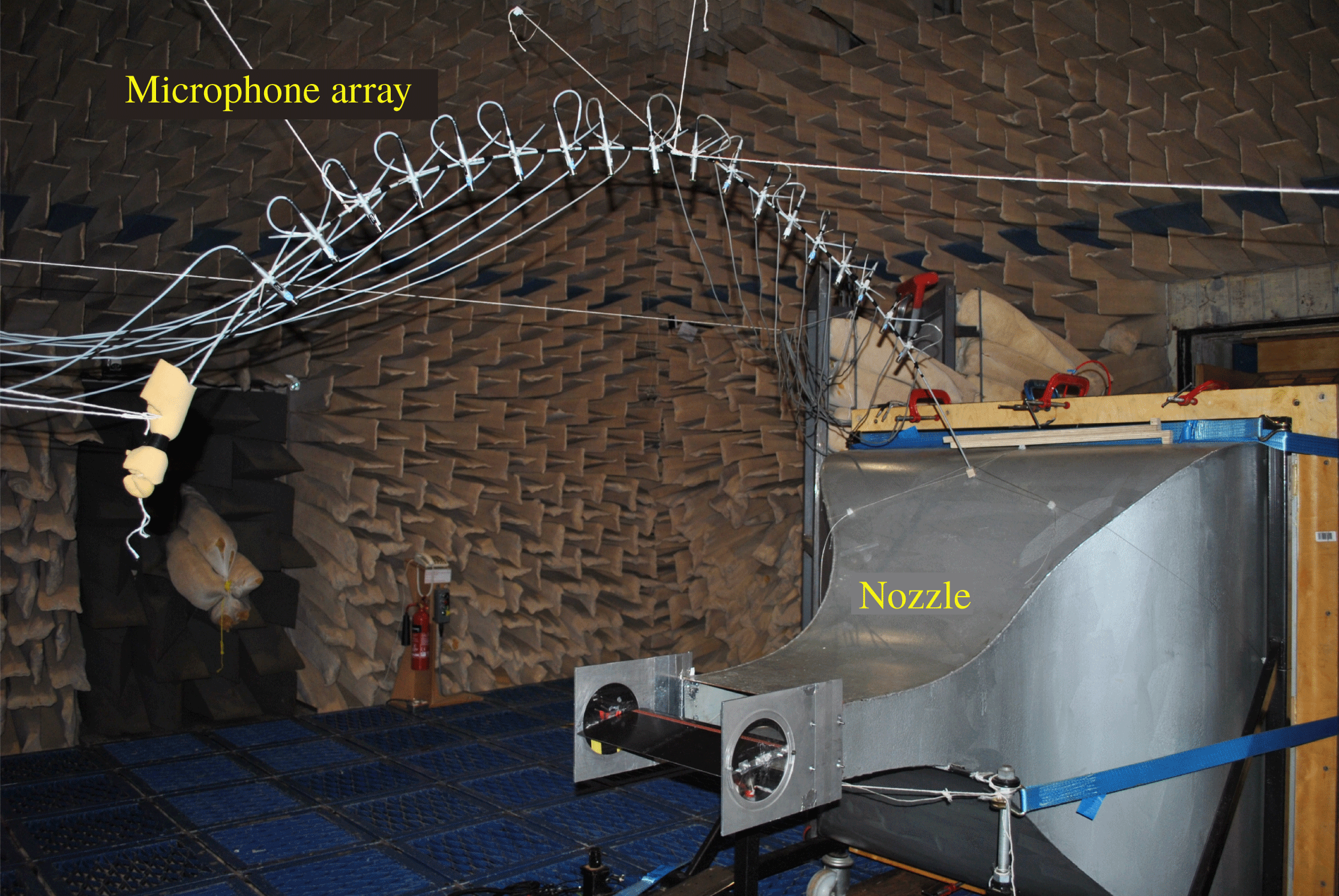
Far-field noise measurements were carried out at the Institute of Sound and Vibration Research’s open-jet wind tunnel facility. The wind tunnel is located within the anechoic chamber, of dimension
 $8~\text{m}\times 8~\text{m}\times 8~\text{m}$
as shown in figure 2. The walls are acoustically treated with glass wool wedges and the cutoff frequency is 80 Hz. The nozzle has dimensions of 150 and 450 mm and provides a maximum flow speed of
 $100~\text{m}~\text{s}^{-1}$
. A detailed description of the wind tunnel, including its characteristics, is presented by Chong, Joseph & Davis (Reference Chong, Joseph and Davis2008). To maintain two-dimensional flow around the flat plate, side plates are mounted to the nozzle exits that will also support the plate in the flow. The mean leading edge of the flat plate is located 150 mm downstream from the nozzle exit.
Photograph of jet nozzle and test set-up inside the ISVR anechoic chamber.
In order to prevent tonal noise generation due to Tollmien–Schlichting waves convecting in the laminar boundary layer, and to ensure complete consistency between the different cases, the flow near the leading edge of the aerofoil was tripped to force transition to turbulence using a rough band of tape of width 1.25 cm located 16.6 % of the chord from the leading edge, on both suction and pressure sides. The tape has roughness of SS 100, corresponding to a surface roughness of
 $140~\unicode[STIX]{x03BC}\text{m}$
. Transition is forced by the use of the trip tape, which is many orders of magnitude rougher than the aerofoil surface, and is therefore highly unlikely to affect transition. Previous noise measurements in our facility have indicated that self-noise is insensitive to the method of tripping.
4.3 Far-field noise measurements
Far-field noise measurements from the flat plate were made using 11, half-inch condenser microphones (B&K type 4189) located at a constant radial distance of 1.2 m from the mid-span of the flat-plate leading edge. These microphones are placed at emission angles between
 $40^{\circ }$
and
 $140^{\circ }$
measured relative to the downstream jet axis. Measurements were carried out for a 10 s duration at a sampling frequency of 50 kHz, and the noise spectra were calculated with a window size of 1024 data points corresponding to a frequency resolution of 48.83 Hz and a bandwidth–time (BT) product of approximately 500, which is sufficient to ensure negligible variance in the spectral estimate at this frequency resolution.
The acoustic pressure at the microphones was recorded at a mean flow velocity (
 $U$
) of
 $60~\text{m}~\text{s}^{-1}$
. Noise measurements are presented in terms of the sound pressure level spectra
 $\text{SPL}(f)$
using the procedure described in Narayanan et al. (Reference Narayanan, Chaitanya, Haeri, Joseph, Kim and Polacsek2015). Sound pressure level reductions,
 $\unicode[STIX]{x0394}\text{SPL}$
, are determined by subtracting the sound pressure level spectra due to the serrated flat plate from that due to the baseline straight edge profile.
4.4 Turbulence characterisation
A bi-planar rectangular grid with overall dimensions of
 $630\times 690~\text{mm}^{2}$
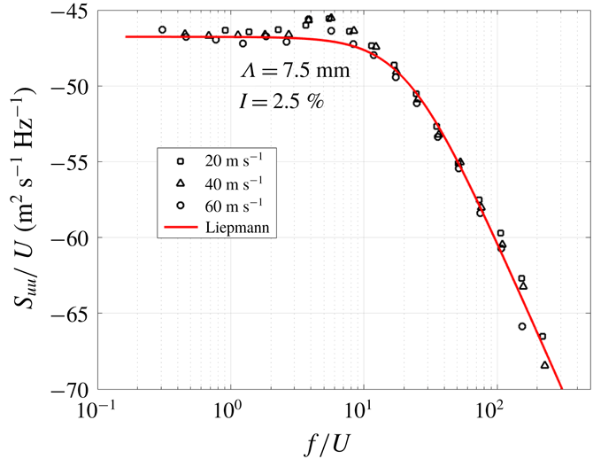
located in the contraction section 75 cm upstream of the nozzle exit was used to generate turbulent flow that provides a velocity spectrum that is a close approximation to homogeneous and isotropic turbulence at the aerofoil leading edge. However, we emphasise that the condition of isotropy is not a key requirement for predicting the noise radiation but only that the velocity spectrum at the aerofoil leading edge is needed for model fitting. A comparison of the streamwise velocity spectra measured at 145 mm from the nozzle exit (
 $S_{uu}/U$
) plotted against
 $f/U$
is compared in figure 3 to the theoretical Liepmann velocity spectrum, where the mean square velocity and integral length scale are chosen to give best fit to the measured data. Close agreement is observed for 2.5 % turbulence intensity and a 7.5 mm streamwise integral length scale.
Comparison between the measured axial velocity spectra and theoretical Liepmann spectra.

4.5 Effect of trailing-edge self-noise
The experimental set-up cannot avoid the generation of trailing-edge self-noise. Figure 4(a) shows the comparison of the sound power levels for baseline and sawtooth serrated aerofoils (
 $c=4$
) with
 $M=0.17$
. Self-noise measurements for the baseline aerofoil are also plotted in the figure demonstrating the influence of self-noise on total noise. We see self-noise becomes increasingly dominant at high frequencies
 $f\gtrsim 6000$
, and thus it appears as if the serration becomes less effective at high frequencies due to the dominance of this self-noise in the total noise measurements. This superficial drop in leading-edge serration performance due to the unavoidable contamination of self-noise was also previously shown by Narayanan et al. (Reference Narayanan, Chaitanya, Haeri, Joseph, Kim and Polacsek2015). As these frequencies are within the range we wish to consider for our experimental and analytical comparison, we must include a simple trailing-edge noise model to the analytical prediction.
Trailing-edge self-noise. (a) Far-field power spectra as a function of frequency for baseline and serrated aerofoils. Self-noise measurements for baseline are obtained when the grid is not placed over the flow nozzle. (b) Comparison of experimetally measured PWL (dashed) and analytic prediction of pressure at
 $\unicode[STIX]{x1D703}=90^{\circ }$
(solid) for trailing-edge self noise.

We use Amiet’s trailing-edge noise model (Amiet Reference Amiet1976) with Howe’s approximation (Howe Reference Howe1998) to Chase’s wall-normal turbulent spectrum (Chase Reference Chase1987), as detailed in Glegg & Devenport (Reference Glegg and Devenport2017, §§ 9–10). This provides us with a far-field spectrum directly above the trailing edge, in the mid-span, of
 $$\begin{eqnarray}\text{SPL}_{TE}=10\log _{10}(S_{pp}(0,r_{t},0,\unicode[STIX]{x1D714}_{t})),\end{eqnarray}$$
where
 $$\begin{eqnarray}S_{pp}(x_{t},y_{t},0,\unicode[STIX]{x1D714}_{t})\approx \unicode[STIX]{x03C0}b\left(\frac{\unicode[STIX]{x1D714}_{t}c_{h}y_{t}}{4\unicode[STIX]{x03C0}c_{0}r_{t}^{2}}\right)^{2}\unicode[STIX]{x1D719}_{pp}(\unicode[STIX]{x1D714}_{t})|{\mathcal{L}}|^{2}.\end{eqnarray}$$
Here
 $(x_{t},y_{t},z_{t})$
are standard Cartesian coordinates centred on the trailing edge,
 $r_{t}$
is the radial distance from the trailing edge,
 $b$
is the chord span and
 $c_{h}$
is the chord length. The frequency,
 $\unicode[STIX]{x1D714}_{t}$
, is assumed to satisfy
 $k_{1}=\unicode[STIX]{x1D714}_{t}/U_{c}$
where
 $U_{c}$
is the convection velocity within the boundary layer,
 $U_{c}\approx 0.7U$
.
 ${\mathcal{L}}$
is Amiet’s generalised lift function (Glegg & Devenport Reference Glegg and Devenport2017, equation (15.2.11)), and
 $\unicode[STIX]{x1D719}_{pp}$
is the expected wall pressure spectrum (Glegg & Devenport Reference Glegg and Devenport2017, equation (9.2.37) denoted as
 $G_{pp}$
). We compare the experimental self-noise measurements to the analytical expression in figure 4(b) seeing good agreement over the range of frequencies of interest, noting oscillations are more dominant in the analytic predictions as these are solely at
 $\unicode[STIX]{x1D703}=90^{\circ }$
.
We make two final notes; first figure 4(a) also illustrates the influence of jet noise from the nozzle is dominant in the experimental measurements at low frequencies,
 $f\lesssim 200$
Hz. The noise for frequencies below 200 Hz is due to typical jet shear layer noise which is also observed in the self-noise spectra. Whereas in the frequency region of 200–400 Hz, the peak in the total noise spectra is due to the interaction of a shedding vortex from the turbulence grid with the aerofoil leading edge. This is absent in the case of self-noise as the measurements are performed without the turbulence grid. However, as these noise sources are unconnected to aerofoil broadband noise, we do not attempt to account for them in the analytic model. Second, as the analytic model assumes an infinite chord, no Kutta condition is imposed at the trailing edge; the effect of the Kutta condition is thought to be important for
 $k^{\ast }c_{h}^{\ast }/(2\unicode[STIX]{x1D6FD}^{2})\leqslant 0.75$
; this also corresponds to low frequencies,
 $f\lesssim 500$
Hz, and is not accounted for in the present analytical model.
5 Results
5.1 Comparison of analytical and experimental results
Here we validate our analytic results by comparing to the experimental measurements for the five leading-edge test geometries, at three different tip-to-root ratios 1, 2 and 4.
We define the total analytic SPL as
 $$\begin{eqnarray}\text{SPL}=10\log _{10}\left(\int _{-\infty }^{\infty }|p^{\ast }|^{2}\unicode[STIX]{x1D6F7}^{(\infty )}(k_{1},k_{3})\,\text{d}k_{3}\right)+\text{SPL}_{TE},\end{eqnarray}$$
where
 $\unicode[STIX]{x1D6F7}^{(\infty )}(k_{1},k_{3})$
is the upstream Liepmann spectrum given by
 $$\begin{eqnarray}\frac{3\overline{u^{\ast \,2}}L^{\ast \,2}}{4\unicode[STIX]{x03C0}}\frac{L^{2}(k_{1}^{2}+k_{3}^{2})}{(1+L^{2}(k_{1}^{2}+k_{3}^{3}))^{5/2}},\end{eqnarray}$$
with
 $L=0.3$
the non-dimensional integral length scale of turbulence (defined as the integral length scale, 7.5 mm, divided by the serration wavelength, 25 mm),
 $L^{\ast }=0.0075$
m the dimensional integral length scale and
 $\overline{u^{\ast }}=0.025U^{\ast }$
is the turbulence intensity (2.5 % of the free-stream velocity,
 $U^{\ast }$
). In (5.1),
 $p^{\ast }$
denotes the dimensional pressure,
 $\unicode[STIX]{x1D70C}_{0}^{\ast }\,U^{\ast \,2}p(r,\unicode[STIX]{x1D703},z)$
, where
 $p$
is the far-field pressure given analytically in (3.17), and
 $\unicode[STIX]{x1D70C}_{0}^{\ast }=1.225~\text{kg}~\text{m}^{-3}$
. The trailing-edge self-noise contribution to the SPL is denoted
 $\text{SPL}_{TE}$
, and is calculated from (4.1).
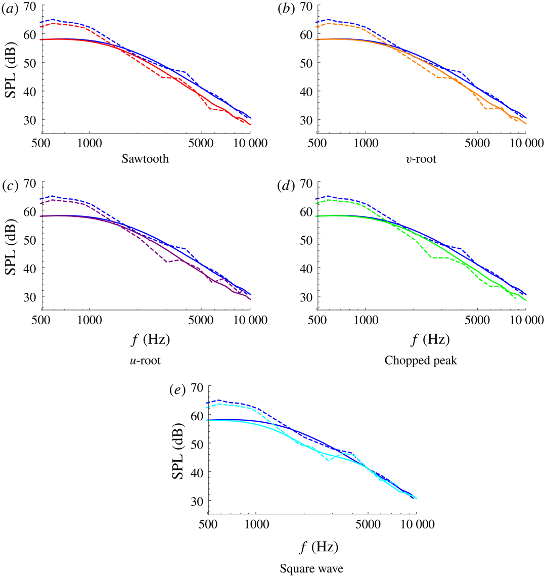
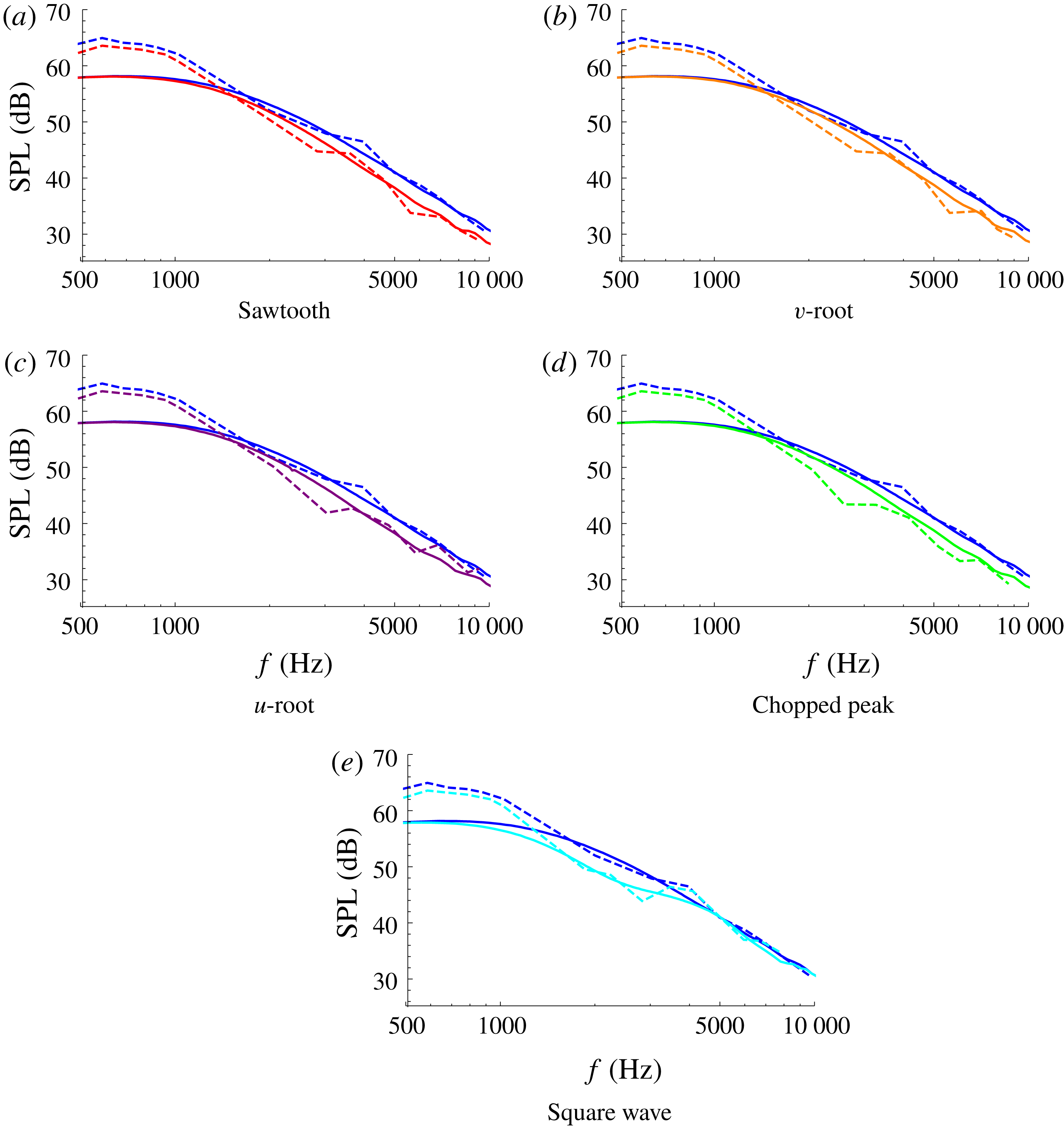
The SPL from analytic results (solid) and experimental measurements (dashed) for each of the five test-case geometries: red (a), orange (b), purple (c), green (d), cyan (e). The straight-edge results are blue throughout. In each case
 $M=0.17$
,
 $c=1$
.
We evaluate (5.1) using the inbuilt NIntegrate feature of Mathematica. For a given
 $k_{1}$
we restrict
 $k_{3}$
values such that
 $|k_{3}|<k_{1}$
, as is expected in the experimentally generated grid turbulence. We sum only the propagating modes of (3.17), the number of which can be easily calculated once given
 $k_{1}$
,
 $k_{3}$
, and
 $M$
.
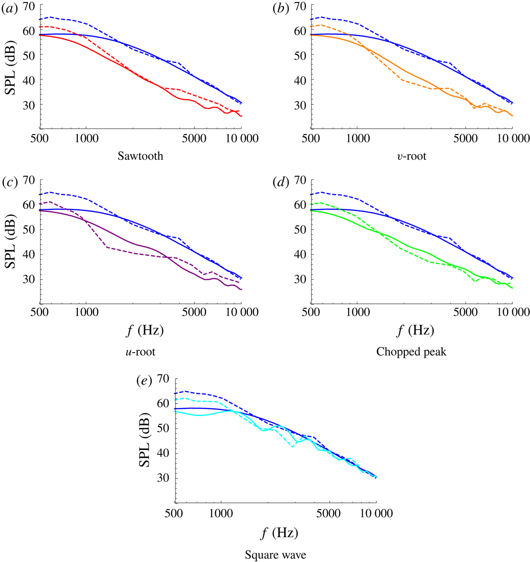
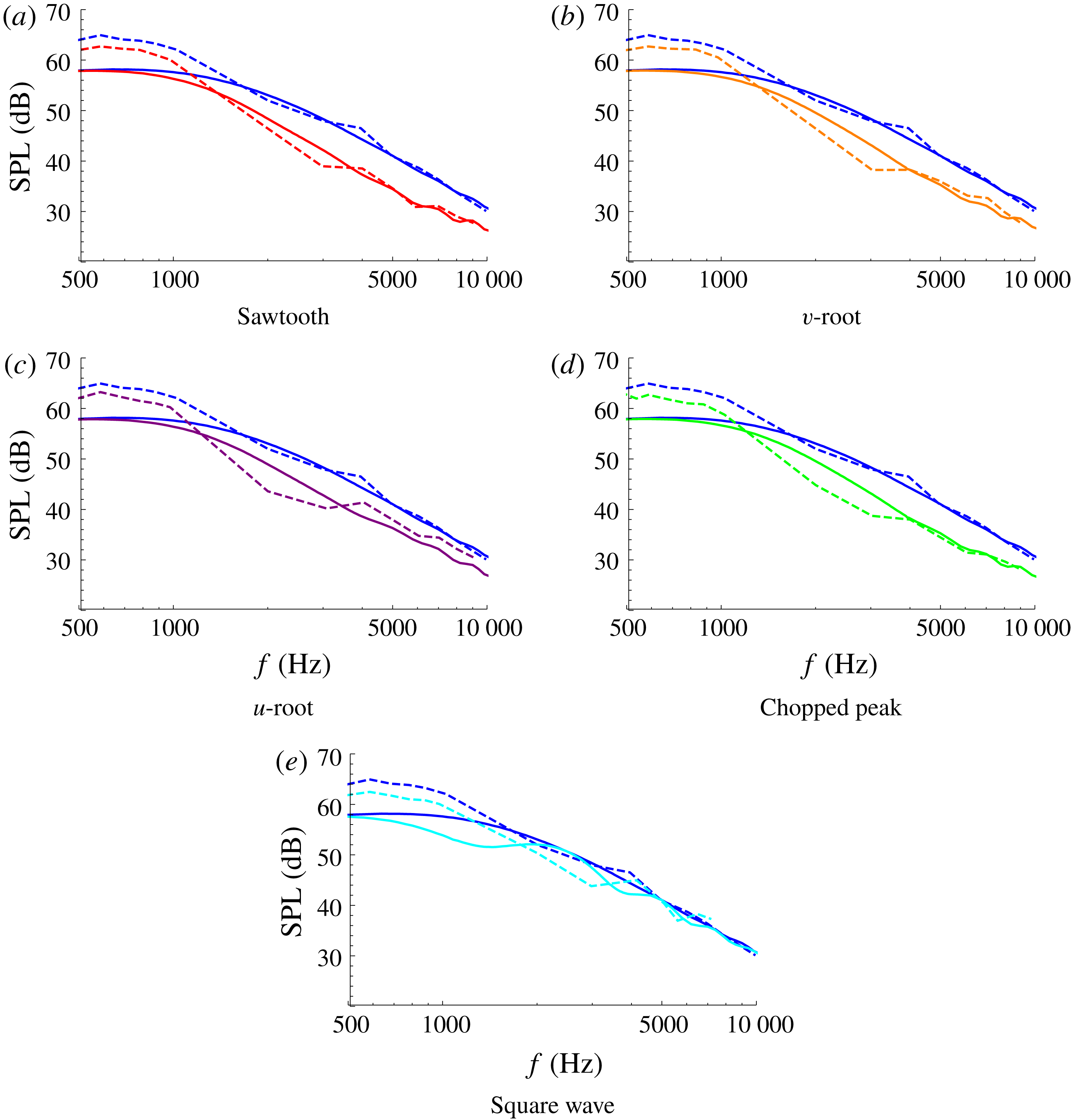
In figures 5–7 we plot the SPL evaluated from the analytic expression (5.1) at
 $r=10$
,
 $\unicode[STIX]{x1D703}=90^{\circ }$
,
 $z=0.5$
, against the experimental measurements from the microphone at
 $\unicode[STIX]{x1D703}=90^{\circ }$
in the plate mid-span. We do so for each of the five leading-edge geometries, at three different tip-to-root ratios,
 $c=1,2,4$
, with
 $M=0.17$
. In each subfigure the straight-edge results are plotted alongside the results for one specific leading-edge geometry. The analytic straight-edged results are calculated by setting
 $c=0.001$
for the relevant geometry. Overall we see good agreement between the analytic solutions and the experimental measurements across a range of tip to root ratios, and for mid- and high-range frequencies
 $f\gtrsim 1000$
Hz. The sawtooth and square wave results have a greatest error of 3 dB, whilst the other geometries have greatest error of 5 dB. We are primarily concerned with the frequency range
 $f\in [1,10]$
kHz as this is the range in which human hearing is most sensitive (frequencies outside of this range are perceived as quieter by the human ear), and it is clear from figures 5–7 serrations can provide good noise reduction in this frequency range.
The SPL from analytic results (solid) and experimental measurements (dashed) for each of the five test-case geometries: red (a), orange (b), purple (c), green (d), cyan (e). The straight-edge results are blue throughout. In each case
 $M=0.17$
,
 $c=2$
.
The SPL from analytic results (solid) and experimental measurements (dashed) for each of the five test-case geometries: red (a), orange (b), purple (c), green (d), cyan (e). The straight-edge results are blue throughout. In each case
 $M=0.17$
,
 $c=4$
.
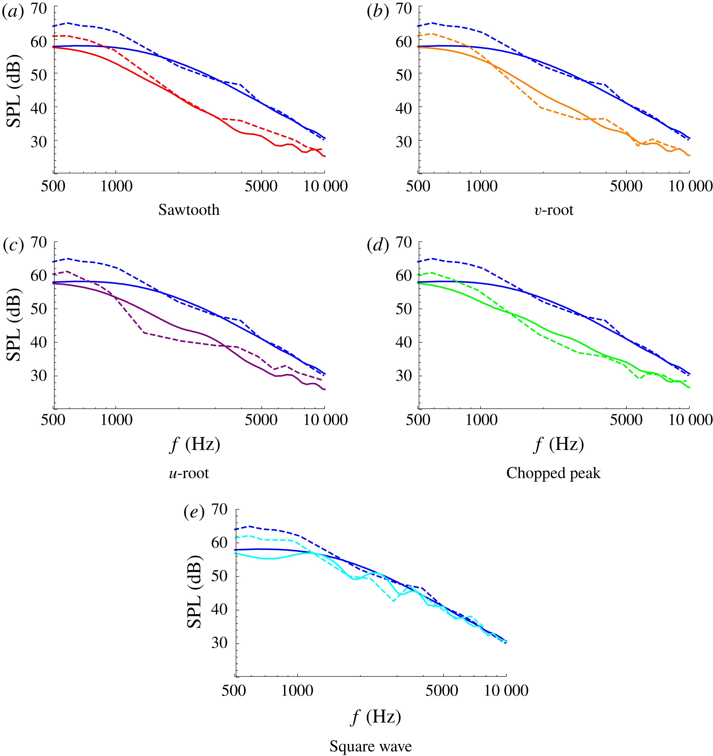
The analytic solutions capture correctly the overall level of noise reduction found experimentally over a wide range of frequencies and correctly capture the trends for varying tip-to-root ratio. With the increase of tip-to-root ratio
 $c$
, the noise reductions for all the designs except for the square wave move towards lower frequencies and the absolute noise reductions compared to the baseline (straight-edged) case is increased. These results are consistent with the previous experimental work of Chaitanya et al. (Reference Chaitanya, Joseph, Narayanan, Vanderwel, Turner, Kim and Ganapathisubramani2017), who demonstrated that the noise reductions are a function of
 $fc/U$
(this will be shown explicitly later in § 5.3). The square wave profile does not show a clear
 $fc/U$
dependence as observed from figures 5(e), 6(e) and 7(e). The analytic solution proposed in this paper is also able to capture these noise reduction trends accurately. However the oscillations in the experimental SPL are not fully captured by the theoretical predictions. These oscillations arise in both the serrated and straight edged cases of the experimental measurements therefore at least in part can be attributed to backscattering effects which are neglected in the theoretical analysis.
A key mechanism permitting good noise reduction from a serrated leading edge is the interference of coherent acoustic fields scattered by the tip and root of the serration (Chaitanya et al.
Reference Chaitanya, Joseph and Ayton2018a
). We see this feature alluded to in the analytical solution through the modal coefficients,
 $E_{n}(\unicode[STIX]{x1D706})$
, given in (3.20), which contain oscillatory functions. A second feature discussed in Ayton & Kim (Reference Ayton and Kim2018) is that of a redistribution of acoustic energy from low cuton modes to higher cutoff modes at large
 $k_{1}c$
values, and is also represented by the modal coefficients
 $E_{n}(\unicode[STIX]{x1D706})$
; at large
 $k_{1}c$
values, corresponding to a large
 $s$
limit in (3.20), we see all
 $E_{n}^{a}$
and
 $E_{n}^{b}$
behave as
 $O(1/s)$
except for very high modes
 $n=O(s)$
which are cutoff. Therefore for these geometries, the sawtooth and slitted
 $v$
-root, as frequency or tip-to-root ratio is increased, energy is transferred from lower cuton modes to higher cutoff modes. The slitted
 $u$
-root and chopped peak geometries, (c) and (d), exhibit only part of their modal coefficients decaying with large
 $s$
, therefore do not redistribute energy as efficiently as the sawtooth and the
 $u$
-root. The square wave, (e), has no modal coefficient parts which decay with large
 $s$
therefore does not redistribute energy at all.
The noise-reduction mechanism for slitted profiles (which includes the square wave geometry considered in this paper) is proposed by Chaitanya & Joseph (Reference Chaitanya and Joseph2018) where optimum slitted profiles are discussed. The reason for this optimum slitted geometry is attributed to the difference in the source strength at the two opposite locations of the slit. A preliminary computational study of the noise reduction mechanism of the leading-edge slits has been performed by Cannard et al. (Reference Cannard, Joseph, Chaitanya and Kim2018) wherein it is shown that narrow slits along an otherwise straight leading edge are able to generate comparatively high source levels at the root through the formation of a secondary streamwise vortex generated along the edge of the slit and then interacting with the root. This secondary feature which is important for slitted profiles is not accounted for in the analytic model, but will be discussed further in § 5.4.
To consider the primary noise-reduction mechanisms of interference and redistribution more closely, we look at the analytically predicted scattered surface pressure along the leading edge of the serration.
5.2 Surface pressure
For simplicity here we restrict to considering single-frequency gusts, i.e. fixed
 $k_{3}$
wavenumbers rather than integrating over a wavenumber spectrum. This will give us a simple idea of how the interference and redistribution mechanisms manifest as a pressure variation on the surface, and how this is affected by oblique gusts.
We calculate the surface pressure from (3.16) where
 $h$
is given by (3.14). By interchanging the integration and differentiation we may express the surface pressure (on the upper surface of the plate) as
 $$\begin{eqnarray}p_{s}(x,0_{+},z)=\mathop{\sum }_{n=-\infty }^{\infty }\frac{1}{2\unicode[STIX]{x03C0}\unicode[STIX]{x1D6FD}\sqrt{-\unicode[STIX]{x1D6FF}-w_{n}}}\int _{-\infty }^{\infty }\frac{\text{e}^{-\text{i}\unicode[STIX]{x1D706}x/\unicode[STIX]{x1D6FD}}E_{n}(\unicode[STIX]{x1D706})}{\sqrt{\unicode[STIX]{x1D706}+w_{n}}}\,\text{d}\unicode[STIX]{x1D706}\text{e}^{\text{i}k_{3}z+2n\unicode[STIX]{x03C0}\text{i}z}\text{e}^{-\text{i}k_{1}M^{2}x/\unicode[STIX]{x1D6FD}^{2}}.\end{eqnarray}$$
As we are interested only in the surface pressure which relates to the dominant contributions to the far-field noise, we restrict the infinite sum to a sum only over a finite number of modes (including all with
 $\text{Im}(w_{n})=0$
). To obtain the solution along the leading-edge of the plate, we evaluate (5.3) at
 $x=\unicode[STIX]{x1D6FD}cF(z)$
, which corresponds to the surface pressure distribution at the leading edge of the flat plate.
5.2.1 Sawtooth profile
We start by considering the surface pressure distribution for the sawtooth profile. Figure 8(a) shows the absolute value of surface pressure distribution along the leading edge of the sawtooth profile for three different values of
 $c=1,2$
and 4 at a fixed
 $M=0.17$
,
 $k_{1}=5$
,
 $k_{3}=0$
. We see that the source strength decreases with the increase of tip-to-root ratio,
 $c$
. This illustrates the redistribution of acoustic energy away from the low propagating modes with the increase of tip-to-root ratio.
Absolute value of surface pressure contributing to outgoing acoustic waves along the leading edge of the sawtooth serrated blade. In each case
 $M=0.17$
,
 $k_{1}=5$
,
 $k_{3}=0$
. Solid:
 $c=1$
, dashed:
 $c=2$
, dotted:
 $c=4$
.
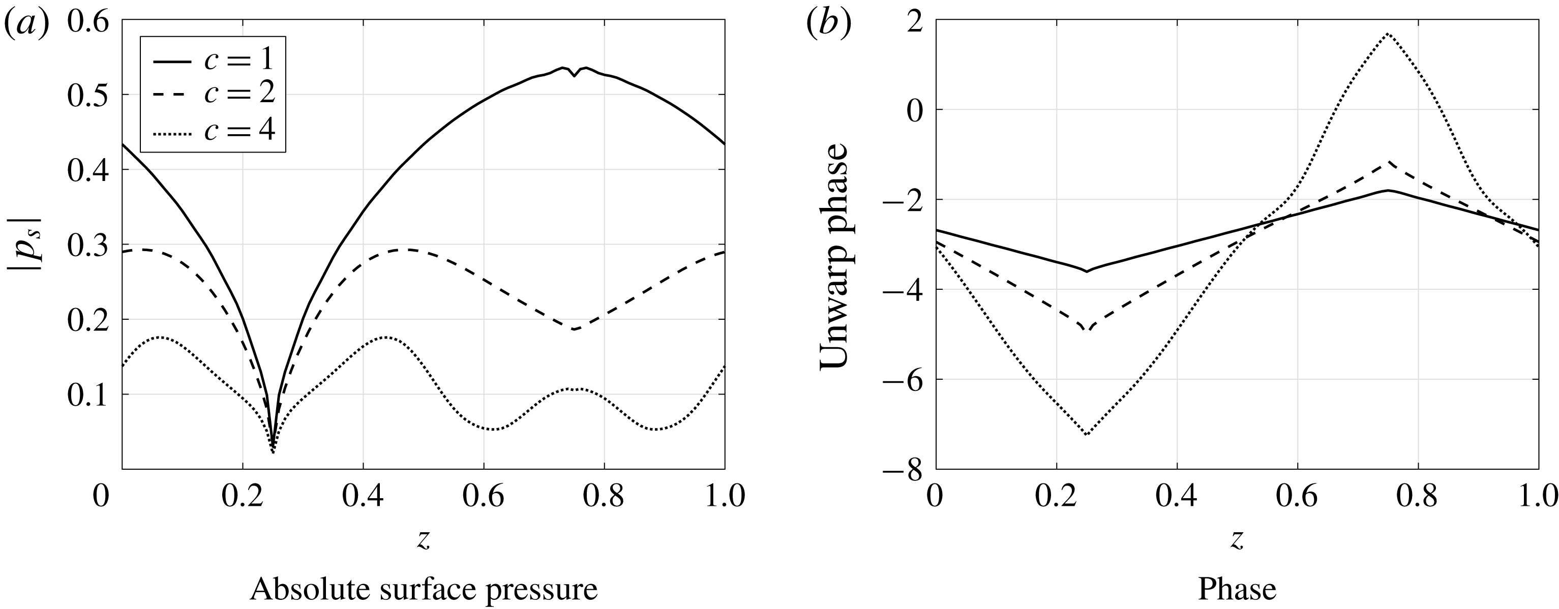
The source strength distribution does not appear to have a clear dominant source region as seen previously by Chaitanya et al. (Reference Chaitanya, Joseph, Narayanan, Vanderwel, Turner, Kim and Ganapathisubramani2017), Turner & Kim (Reference Turner and Kim2017). Turner & Kim (Reference Turner and Kim2017) showed that the root of the serrated leading edge is the dominant noise source due to the presence of a secondary horseshoe-like vortex system generated by the serrated leading edge, which alters the upstream velocity field, thereby enhancing the surface pressure at the serration root. However, the current (linear) mathematical model does not capture these secondary flow features, which are a purely nonlinear feature. This nonlinear feature is not the primary noise-reduction mechanism of sawtooth serrated leading-edge profiles; the primary noise-reduction mechanism, as demonstrated by many authors previously (Kim et al.
Reference Kim, Haeri and Joseph2016; Chaitanya et al.
Reference Chaitanya, Joseph, Narayanan, Vanderwel, Turner, Kim and Ganapathisubramani2017; Ayton & Kim Reference Ayton and Kim2018), is the destructive interference along the serrated profile. This is further demonstrated by the analytic solution by the phase distribution along the leading edge of the sawtooth profile for three different values of
 $c=1,2$
and 4 at a fixed
 $M=0.17$
,
 $k_{1}=5$
,
 $k_{3}=0$
in figure 8(b). The phase variation along the sawtooth profile behaves similarly to the geometry of the profile itself, for all the three tip-to-root ratios. This demonstrates the phase variation due to incoming parallel gust along with the variable surface pressure distribution results in destructive interference phenomena. This is consistent with the simple phase model hypothesis proposed by Chaitanya et al. (Reference Chaitanya, Joseph, Narayanan, Vanderwel, Turner, Kim and Ganapathisubramani2017) where
 $\text{e}^{-k_{1}x}$
is the key term responsible for noise reductions by serrated leading-edge profiles.
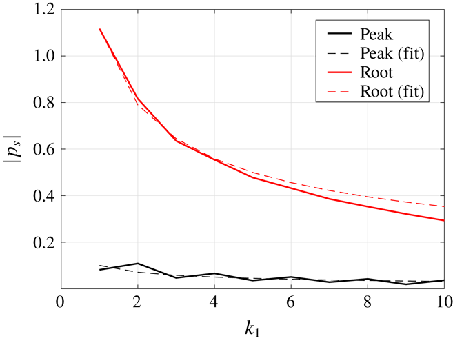
Figure 9 shows the variation of absolute surface pressure at two locations, the tip and the root on the leading edge of the sawtooth profile, with
 $k_{1}$
at
 $M=0.17$
,
 $k_{3}=0$
,
 $c=1$
. Also plotted is the
 $1/\sqrt{k_{1}}$
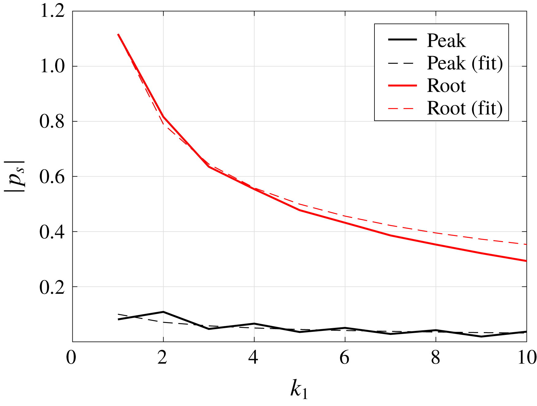
curve for the two locations. The absolute surface pressure shows a
 $1/\sqrt{k_{1}}$
dependence which is consistent with the high-frequency approximation of the Sommerfeld half-plate problem. The two locations considered here have similar characteristics to those of the flat plate and demonstrate the local gradient of the serrated edge is a key factor governing the surface pressure distribution.
Variation of absolute value of surface pressure contributing to outgoing acoustic waves at the root (black) and peak (red) locations with respect to
 $k_{1}$
for
 $M=0.17$
,
 $k_{3}=0$
,
 $c=1$
. Dashed:
 $1/\sqrt{k}_{1}$
fit.
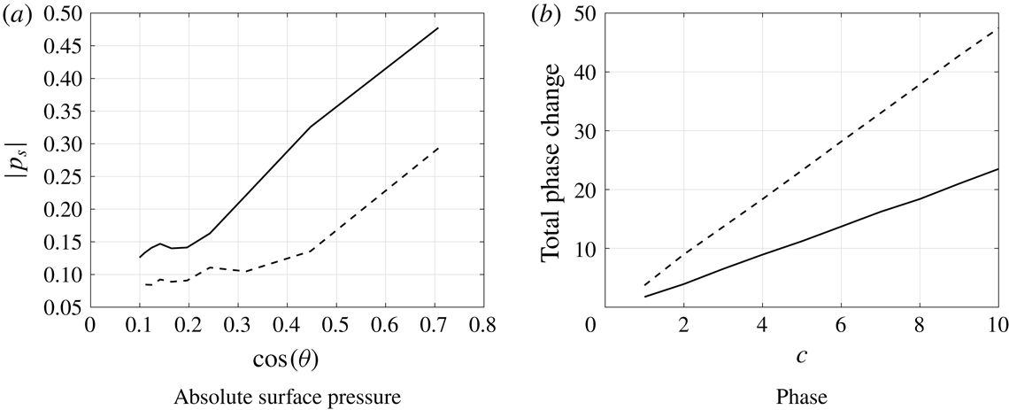
To demonstrate this explicitly, variation of absolute surface pressure at the mid-location of the oblique edge for the sawtooth profile is predicted for varying tip to root ratio
 $c=1$
to 10. Figure 10(a) shows the variation of absolute surface pressure plotted against the cosine of the inclination angle
 $\unicode[STIX]{x1D703}$
for
 $k_{1}=5,10$
respectively. The surface pressure along the oblique edge seems to be proportional to
 $\cos \unicode[STIX]{x1D703}$
which is consistent with Roger & Carazo (Reference Roger and Carazo2010). They suggested an analytical expression to predict the aerofoil noise due to sinusoidal gust when the aerofoil/blade is swept relative to the free-stream direction. According to their analysis, the surface pressure is proportional to
 $\cos \unicode[STIX]{x1D703}$
, where
 $\unicode[STIX]{x1D703}$
is the sweep angle. The larger the inclination angle of the serration, i.e. the larger the tip-to-root ratio
 $c$
, the more the surface pressure is reduced (proportional to
 $\cos \unicode[STIX]{x1D703}$
).
Variation of absolute value of surface pressure contributing to outgoing acoustic waves at the mid location of sawtooth serrated profile with respect to
 $c$
. In each case
 $M=0.17$
,
 $c=1$
,
 $k_{3}=0$
. Solid:
 $k_{1}=5$
, dashed:
 $k_{1}=10$
.
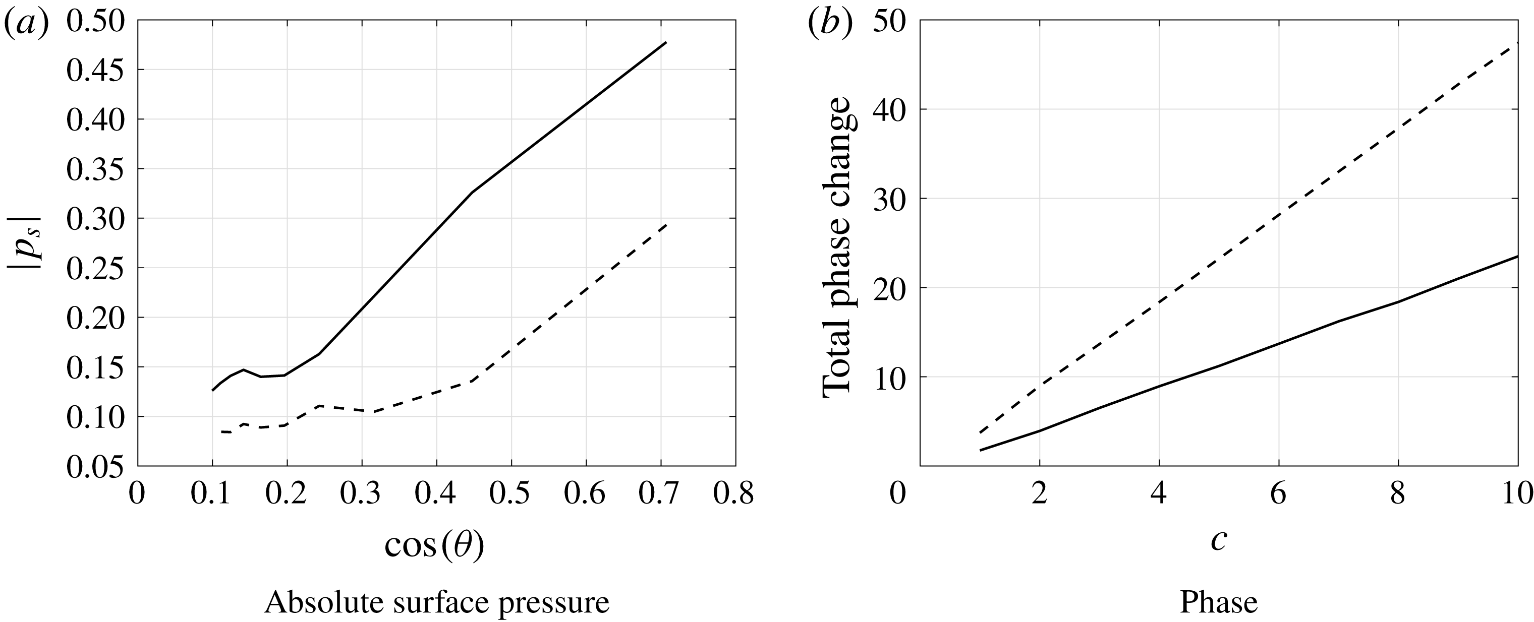
The total phase change along the sawtooth profile is also calculated for varying tip to root ratio of
 $c=1$
to 10 and plotted in figure 10(b) for
 $k_{1}=5,10$
. The total phase change is seen to be proportional to
 $k_{1}$
and the tip to root ratio
 $c$
, where the rapid phase change along the oblique surface is a key noise reduction mechanism for serrated leading-edge profiles. These observations are consistent with the Kim et al. (Reference Kim, Haeri and Joseph2016) who proposed the two dominant noise-reduction mechanisms. One is due to a source cutoff effect arising from the obliqueness of the inclined leading edge and the second is due to interference between the sources along the serrated leading edge.
These observations demonstrate the current generalised model proposed in this paper captures the primary noise-reduction mechanism of sawtooth leading-edge profiles.
5.2.2 Other profiles
In figure 11 we see the leading-edge surface pressures for
 $k_{3}=0$
at a fixed frequency
 $k_{1}=5$
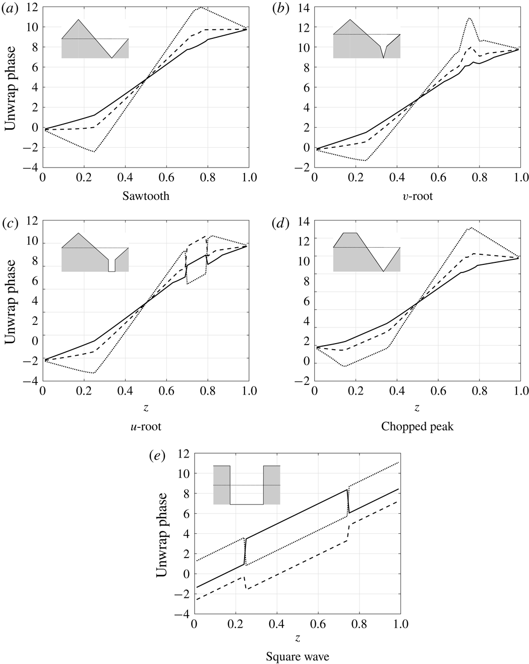
for the remaining four test-case profiles. We see in the cases of the triangular-based geometries (a–c) as the tip to root ratio is increased the overall magnitude of the absolute surface pressure is reduced which is consistent with the sawtooth profile as seen in figure 8. This illustrates the redistribution of acoustic energy away from the low propagating modes towards higher cutoff modes. Similarly the second mechanism of interference is illustrated by figure 12 through the phase distribution along the leading-edge profiles. All the phase variations are consistent with the geometry of the serrated profile.
Absolute value of surface pressure contributing to outgoing acoustic waves along the leading edge of the serrated blade. In each case
 $M=0.17$
,
 $k_{1}=5$
,
 $k_{3}=0$
. Solid;
 $c=1$
, dashed;
 $c=2$
, dotted;
 $c=4$
. The shaded shape in each panel denotes the leading-edge geometry.
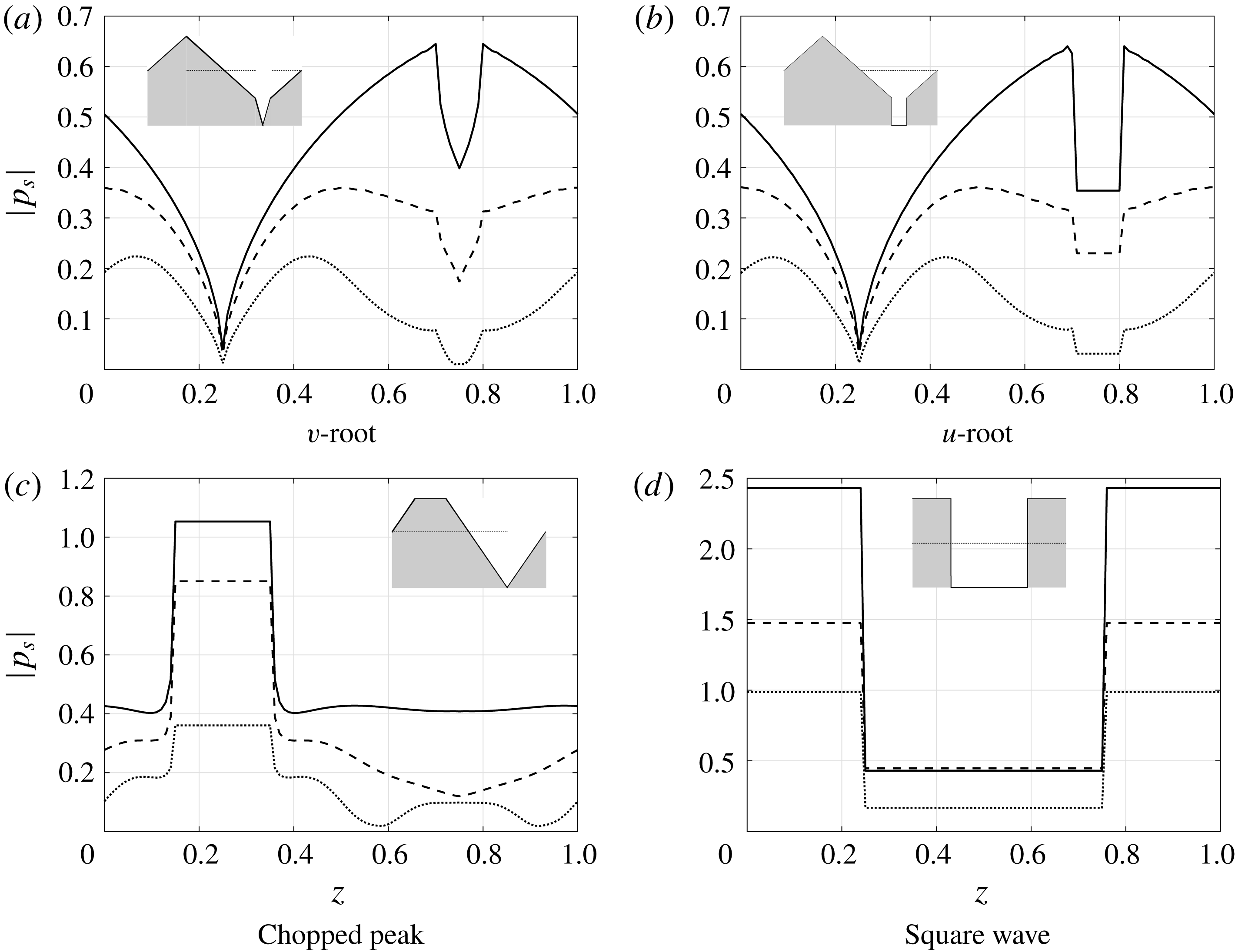
The characteristics of the square wave profile are different compared to the other triangular-based geometries. For the square wave, there are principally only two deviations of surface pressure along the leading edge for a serrated case compared to the straight case. These deviations can efficiently destructively interfere with each other in the far field, much more effectively than the multiple variable pressures associated with the triangular-based geometries, but this will only happen when the two source strengths are specifically tuned in such a way that they both interfere destructively. This has been demonstrated by Chaitanya et al. (Reference Chaitanya, Joseph and Ayton2018a ). The square wave illustrates how it is not necessary to have a rapidly varying pressure along the leading edge, but important to have variable pressure at the tip and root regions to enable a good destructive interference in the far field. We discuss the unique features of the square wave geometry further in § 5.4.
Argument of surface pressure contributing to outgoing acoustic waves along the leading edge of the serrated blade. In each case
 $M=0.17$
,
 $k_{1}=5$
,
 $k_{3}=0$
. Solid;
 $c=1$
, dashed;
 $c=2$
, dotted;
 $c=4$
. The shaded shape in each panel denotes the leading-edge geometry.

5.2.3 Influence of oblique gusts
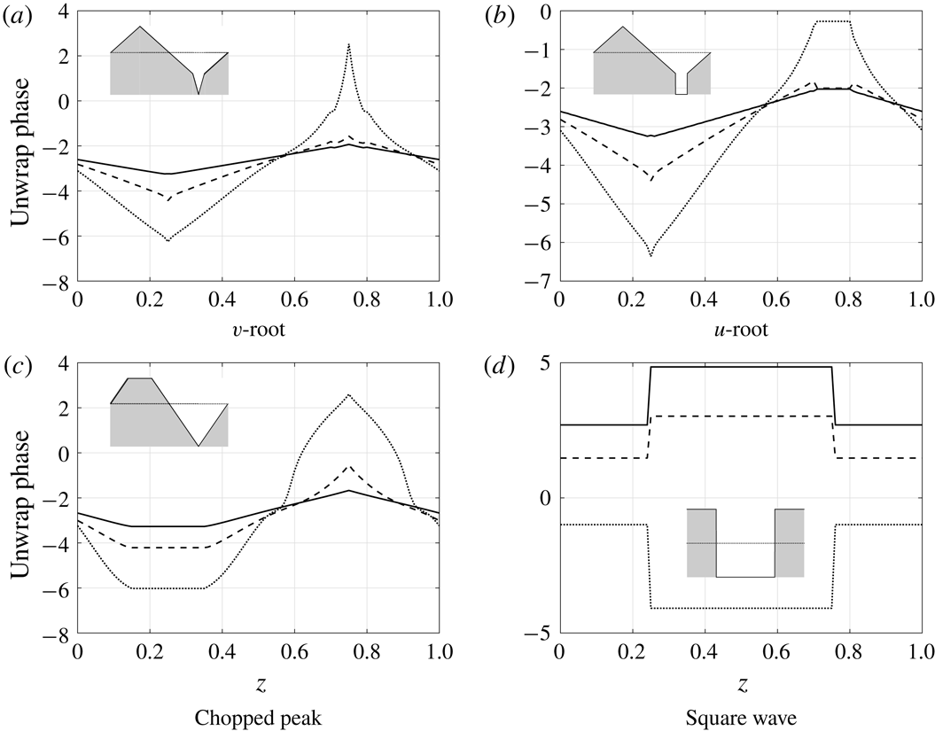
We now consider an oblique gust impinging onto the serrated profiles. The absolute value of the surface pressures and the phase variations along the leading edge are plotted in figures 13 and 14 for three different tip-to-root ratios
 $c=1,2,4$
at
 $M=0.17$
,
 $k_{1}=5$
,
 $k_{3}=10$
. The absolute surface pressures are consistently lower than those for a parallel gust of
 $k_{3}=0$
but continue the trend with increasing tip-to-root ratio as seen previously for the parallel gust in figure 8(a). This indicates that whilst the redistribution mechanism is similar for both oblique and non-oblique gusts, the influence on non-oblique gusts is more significant to the overall noise levels.
Absolute value of surface pressure contributing to outgoing acoustic waves along the leading edge of the serrated blade. In each case
 $M=0.17$
,
 $k_{1}=5$
,
 $k_{3}=10$
. Solid;
 $c=1$
, dashed;
 $c=2$
, dotted;
 $c=4$
.

Argument of surface pressure contributing to outgoing acoustic waves along the leading edge of the serrated blade. In each case
 $M=0.17$
,
 $k_{1}=5$
,
 $k_{3}=10$
. Solid;
 $c=1$
, dashed;
 $c=2$
, dotted;
 $c=4$
. The shaded shape in each panel denotes the leading-edge geometry.
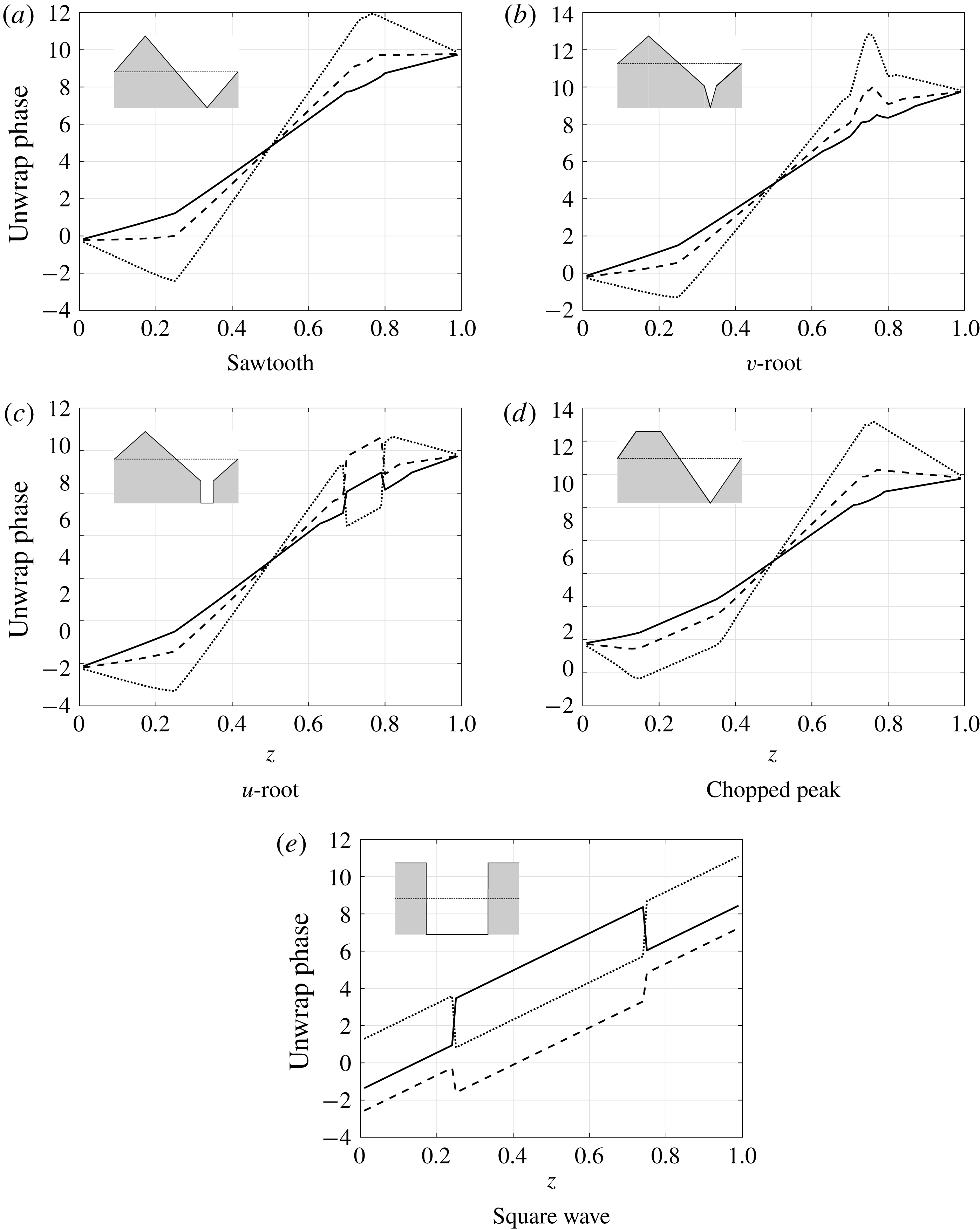
The phase distribution for oblique gusts is significantly different compared to non-oblique gusts. The edge parallel to the oblique gust will be excited in phase as seen in figure 14(a) in the ranges
 $z\in [0,0.25]$
and
 $z\in [0.75,1]$
in the case of
 $c=2$
; here the inclination angle (
 $\tan ^{-1}c$
) of the oblique edge is equal to the oblique angle of the gust (
 $\tan ^{-1}k_{3}/k_{1}$
). This reduces the effectiveness of the phase interference along the leading edge, however, only half the leading-edge profile is excited in phase, so the other half will interfere destructively therefore some noise reduction will occur. The overall far-field radiated pressure is the sum of pressures due to all oblique wavenumber gusts impinging of the leading-edge profiles, therefore this particular case of an oblique gust parallel to a section of the serration with a slightly reduced interference ability is an anomaly.
5.3 Noise-reduction variation with observer angle
In this section we consider the effect of varying Mach number and observer angle on the leading-edge far-field noise reduction for our different leading-edge geometries by using the analytic solution. Here the noise reductions for various leading-edge geometries are calculated with respect to baseline (straight leading edge). Note this does not include the contamination of trailing-edge noise, thus is governed by (3.17). We initially focus on
 $k_{3}=0$
to illustrate the key features of the scattering of a single gust by the leading edge. We then integrate over all spanwise wavenumbers using the Liepmann spectrum to obtain predictions for realistic noise reductions in a turbulent stream.
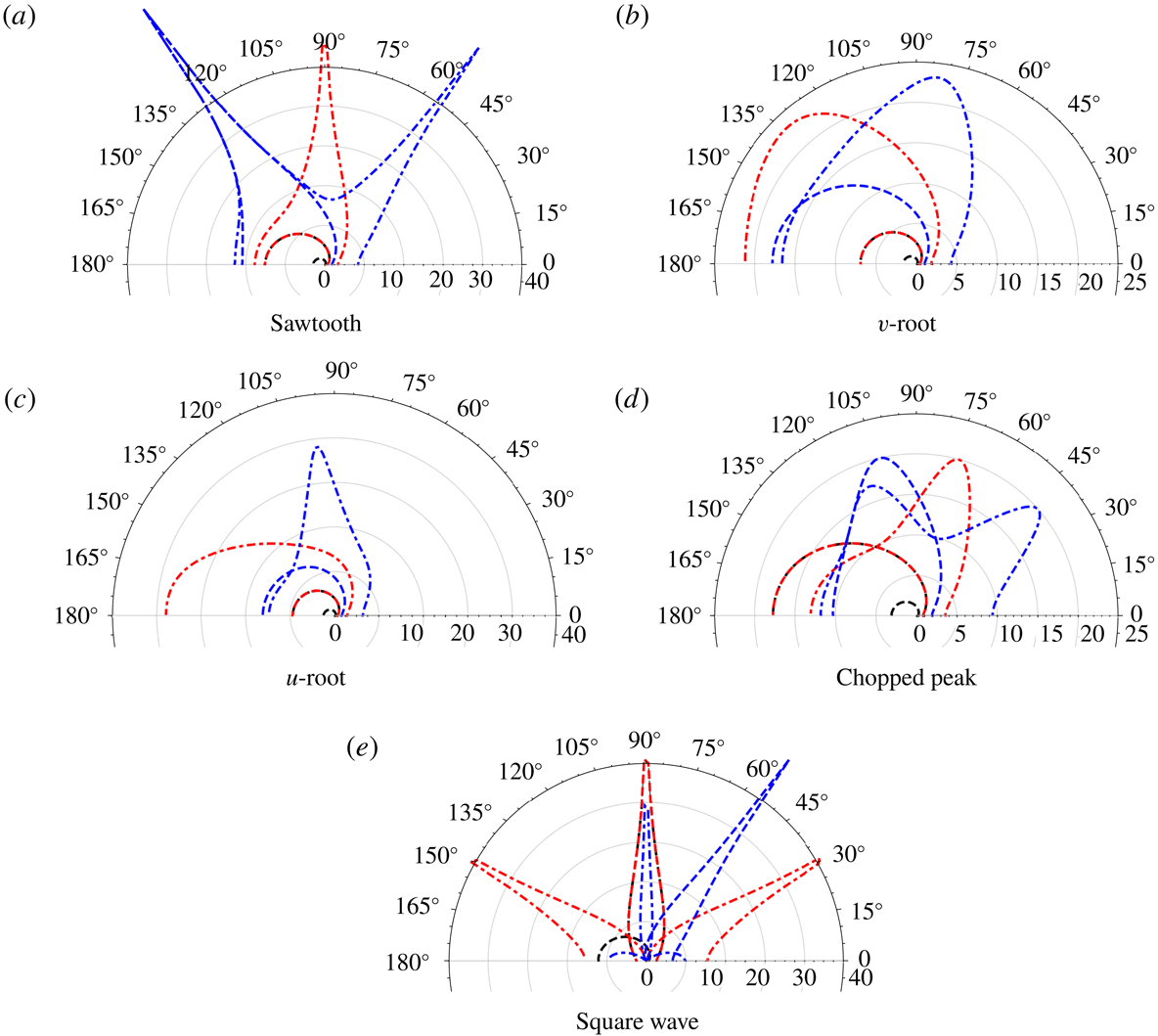
Figure 15(a–e) shows the directivity of noise reduction in dB for various leading-edge configurations at two different tip to root ratio
 $c$
of 1, 2 and three different non-dimensional frequencies
 $k_{1}$
of
 $\unicode[STIX]{x03C0}$
,
 $2\unicode[STIX]{x03C0}$
and
 $3\unicode[STIX]{x03C0}$
, at a fixed Mach number
 $M=0.17$
, and fixed
 $k_{3}=0$
. Similarly, Figure 16(a–e) shows the directivity of noise reduction in dB at a fixed Mach number
 $M=0.5$
and fixed
 $k_{3}=0$
. The rationale behind considering these frequencies is based on the previous work of Chaitanya et al. (Reference Chaitanya, Joseph, Narayanan, Vanderwel, Turner, Kim and Ganapathisubramani2017), where the authors demonstrated the noise reductions are functions of tip-to-root distance
 $c$
and hydrodynamic wavelength
 $U/f$
, i.e. functions of
 $k_{1}c$
. This is illustrated in the analytical solutions as we see a good overlap of the directivity curves in figures 15 and 16 for a fixed
 $k_{1}c=2\unicode[STIX]{x03C0}$
.
Noise reduction (dB) with respect to baseline (straight edge) in the blade mid-span,
 $r=10$
,
 $M=0.17$
,
 $k_{3}=0$
. Dashed:
 $c=1$
, dot-dashed:
 $c=2$
. Black:
 $k_{1}=\unicode[STIX]{x03C0}$
, red:
 $k_{1}=2\unicode[STIX]{x03C0}$
, blue:
 $k_{1}=3\unicode[STIX]{x03C0}$
.

Noise reduction (dB) with respect to baseline (straight edge) in the blade mid-span,
 $r=10$
,
 $M=0.5$
,
 $k_{3}=0$
. Dashed:
 $c=1$
, dot-dashed:
 $c=2$
. Black:
 $k_{1}=\unicode[STIX]{x03C0}$
, red:
 $k_{1}=2\unicode[STIX]{x03C0}$
, blue:
 $k_{1}=3\unicode[STIX]{x03C0}$
.
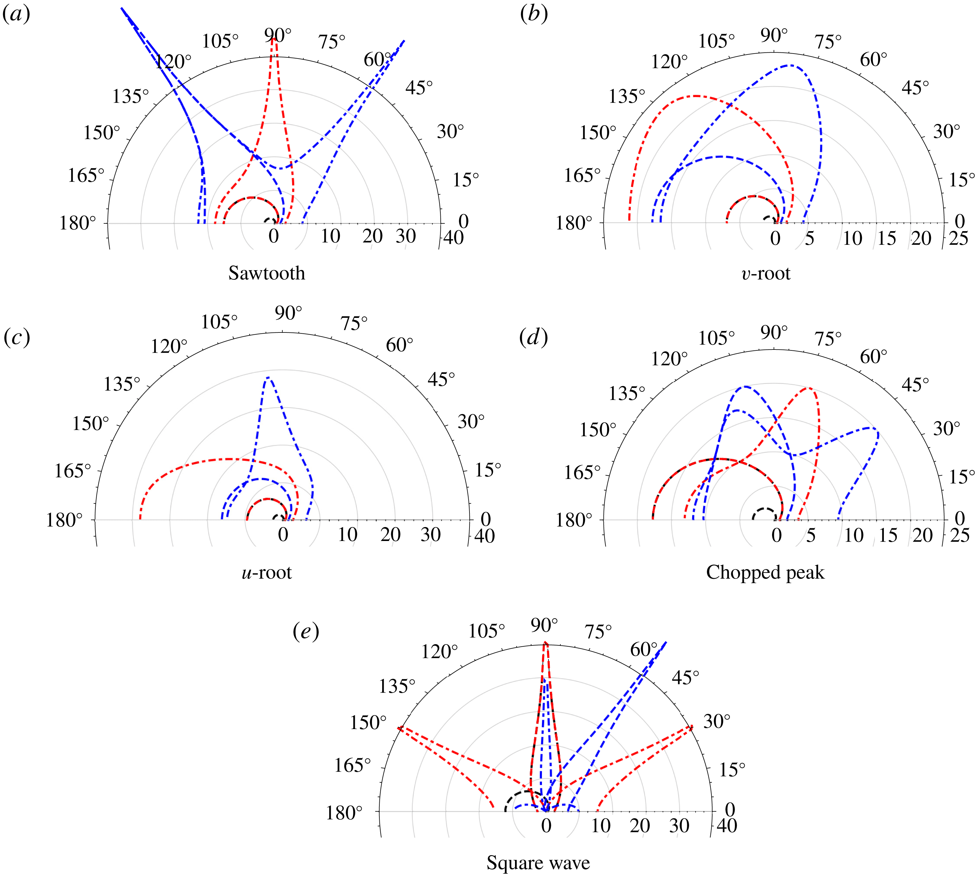
Figures 15 and 16 demonstrate the directivity patterns are strong functions of non-dimensional frequency
 $k_{1}c$
and Mach number
 $M$
. Optimum noise reductions of up to 40 dB are observed at specific observer angles, conversely at other specific observer angles no noise reductions are observed. These oscillations are a result of the strong interference of the scattered acoustic fields from different sources located along the leading edge of the aerofoil. These interference patterns are functions of the path difference between these leading-edge sources and the far-field observer location, convective sound speed, flow Mach number
 $M$
. For higher Mach numbers and greater values of
 $k_{1}c$
the oscillations for a given geometry increase due to rapid phase changes resulting in more directivity lobes. This is particularly evident in the case of square wave where we have two dominant sources on either end of the slit.
Since figures 15 and 16 account only for
 $k_{3}=0$
, the constructive (no noise reduction) or destructive (large noise reduction) interference is over-exaggerated, as these specific angles will differ with different values of
 $k_{3}$
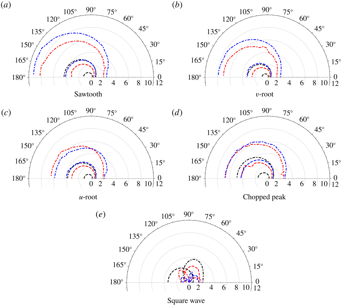
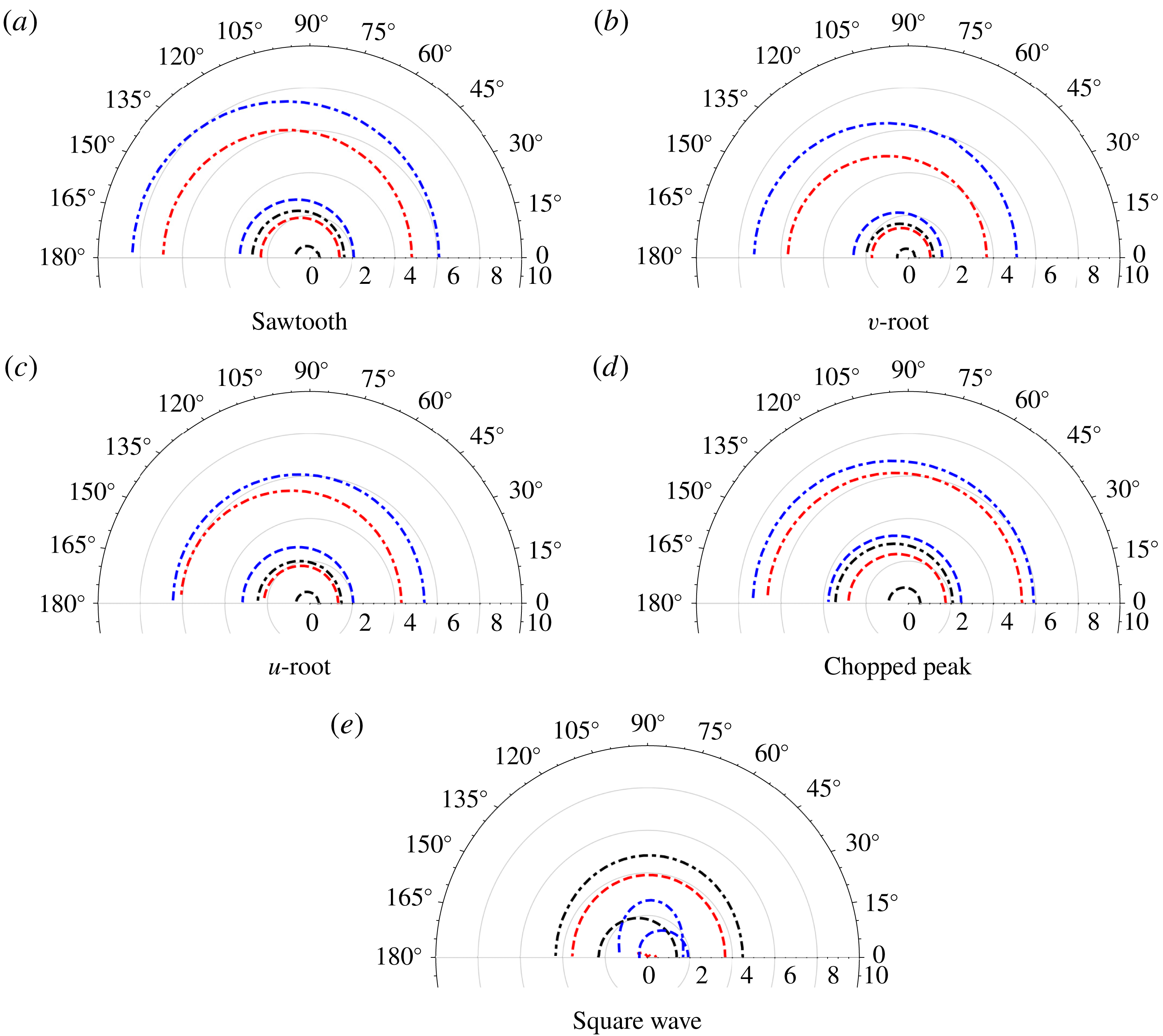
. To consider the noise reduction in a fully turbulent stream, we integrate the individual
 $k_{3}$
components over the Liepmann spectrum to obtain figures 17 and 18. We see clearly the noise-reduction directivities are now much more uniform with far fewer oscillations. The noise reductions still adhere to being functions of
 $k_{1}c$
, although due to the additional length scale of the incident turbulence,
 $L$
, there is now not perfect overlap at fixed
 $k_{1}c=2\unicode[STIX]{x03C0}$
.
Noise reduction (dB) with respect to baseline (straight edge) in the blade mid-span,
 $r=10$
,
 $M=0.17$
, integrated over a Liepmann spectrum of
 $k_{3}$
wavenumbers with
 $L=0.28$
. Dashed:
 $c=1$
, dot-dashed:
 $c=2$
. Black:
 $k_{1}=\unicode[STIX]{x03C0}$
, red:
 $k_{1}=2\unicode[STIX]{x03C0}$
, blue:
 $k_{1}=3\unicode[STIX]{x03C0}$
.
Noise reduction (dB) with respect to baseline (straight edge) in the blade mid-span,
 $r=10$
,
 $M=0.5$
, integrated over a Liepmann spectrum of
 $k_{3}$
wavenumbers with
 $L=0.28$
. Dashed:
 $c=1$
, dot-dashed:
 $c=2$
. Black:
 $k_{1}=\unicode[STIX]{x03C0}$
, red:
 $k_{1}=2\unicode[STIX]{x03C0}$
, blue:
 $k_{1}=3\unicode[STIX]{x03C0}$
.
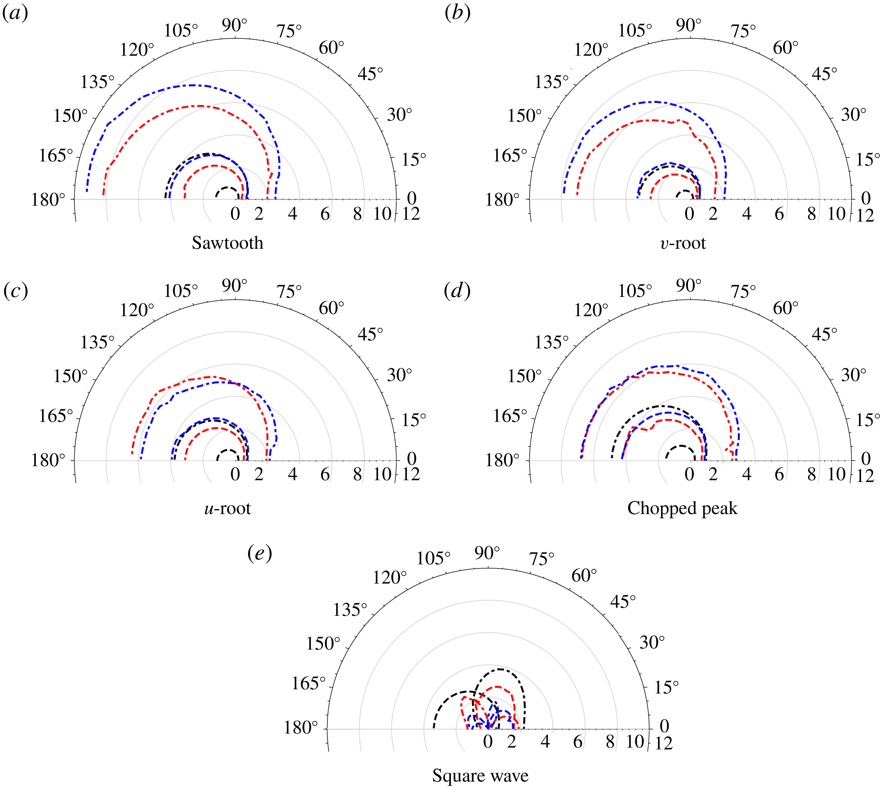
What we also observe from figures 17 and 18 is that leading-edge geometries with straight sections, the
 $u$
-root (c), chopped peak (d) and square wave (e), tend to a limited noise-reduction value (increasing
 $k_{1}c$
does not continue to decrease noise), whereas the sawtooth (a) and
 $v$
-root (b) continue to reduce leading-edge noise with increasing
 $k_{1}c$
. This is consistent with Chaitanya et al. (Reference Chaitanya, Joseph, Narayanan, Vanderwel, Turner, Kim and Ganapathisubramani2017), where the noise reductions for a sawtooth edge are shown to be proportional to the Strouhal number relative to the serration amplitude i.e.
 $k_{1}c$
. Similarly as shown by Chaitanya et al. (Reference Chaitanya, Joseph and Ayton2018a
), for the cases of the
 $u$
-root (c), chopped peak (d) and square wave (e), additional noise-reduction mechanisms i.e. destructive interference occurs between the dominant sources as their strengths becomes comparatively equal due to their straight sections. The square wave once again behaves most distinctly in comparison with the other four triangular-based geometries. Peak noise reductions for the square wave occur when the two sources are
 $180^{\circ }$
out of phase which occurs when the non-dimensional frequency
 $k_{1}c$
becomes
 $2(2n-1)\unicode[STIX]{x03C0}$
, where
 $n$
is any given integer. Hence, the cases
 $c=1$
,
 $k_{1}=2\unicode[STIX]{x03C0}$
and
 $c=2$
,
 $k_{1}=\unicode[STIX]{x03C0}$
demonstrate the greatest noise reductions for the square wave profile. We shall discuss the square wave, and more general slitted geometries further in the following section.
Finally, an important idea to be taken away from the comparison of the single-frequency noise reductions of figures 15 and 16, and the full homogeneous turbulence reductions of figures 17 and 18, is that the noise reductions could depend strongly on the structure of the incident turbulence. For example, if the
 $k_{3}=0$
mode strongly dominated (i.e. the incident turbulence was not homogeneous and isotropic), we would expect the total noise reductions to be more oscillatory and have observer angles where constructive and destructive interference mirrors that from figures 15 and 16. Therefore in a practical setting, knowledge of the upstream turbulence could be key to assessing the total noise reduction due to a serrated leading edge and its variation with observer angle.
5.4 Slitted profiles and the applicability of the analytical model
We have consistently seen the square wave profile behave differently to the triangular based profiles. This section discusses some of the features specific to the square wave as illustrated by figure 1(e).
For a general slitted profile, the leading-edge function
 $F(z)$
is given by
 $$\begin{eqnarray}\text{slitted}\quad F_{s}(z)=\frac{1}{4}\left\{\begin{array}{@{}ll@{}}-1,\quad & z\in [0,a)\\ +1,\quad & z\in (a,b)\\ -1,\quad & z\in (b,1],\end{array}\right.\end{eqnarray}$$
where
 $b-a$
is the width of the slit relative to total wavelength of the serration.
Optimum slitted serration profiles have previously been discussed by Chaitanya et al. (Reference Chaitanya, Narayanan, Joseph and Kim2016), and the additional nonlinear noise-reduction mechanism is discussed by Chaitanya et al. (Reference Chaitanya, Joseph, Narayanan and Kim2018b
), Chaitanya & Joseph (Reference Chaitanya and Joseph2018). This mechanism is due to secondary flow structures which, as mentioned earlier, are not captured by current analytic formulation. Also shown by Cannard et al. (Reference Cannard, Joseph, Chaitanya and Kim2018), narrow slits (small values of
 $b-a$
) are able to generate comparatively high source levels at the root through the formation of a secondary streamwise vortex generated along the edge of the slit and then interacting with the root. These secondary flow structures, which are significant for the noise-reduction capabilities of slitted profiles, are only captured by the nonlinear equations whereas the current analytic formulation is linear. Having said this, the current formulation is capable of capturing the primary noise reduction mechanism i.e. redistribution of energy and phase cancellation along the leading edge of the profile where there are no secondary flow structures present which changes the surface pressure distribution.
In this section, by comparing the experimental data for slitted profiles to the linear analytic model, we are able to quantify the effect of this secondary flow feature. Specifically, we consider three slitted profiles given by
 $(a,b)=(0.28,0.72)$
, (0.435, 0.565), (0.45, 0.55) which correspond to slits whose ratios of lengths between the back edge and front edge of the profile,
 $(b-a)/2a$
equals to 0.78, 0.15 and 0.11 respectively.
Sound pressure level reduction (
 $\unicode[STIX]{x0394}\text{SPL}$
) comparisons for a slitted profile for three width ratios of 0.78, 0.15 and 0.11, at jet velocity of
 $60~\text{m}~\text{s}^{-1}$
. Black: = 0.78, Red: = 0.15, Blue = 0.11.
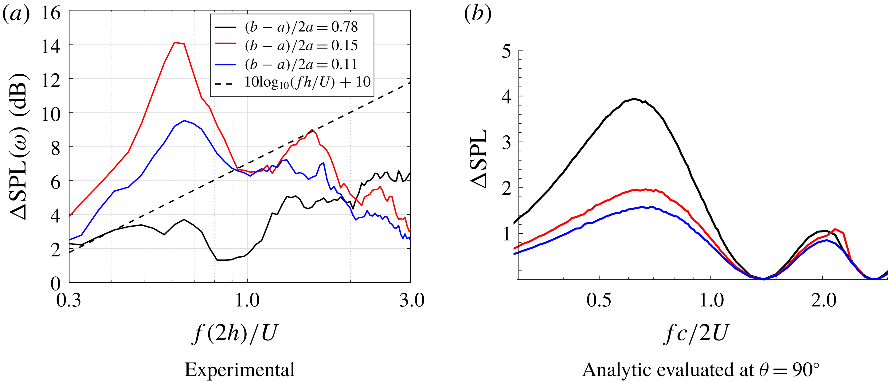
Figure 19 shows the comparison of the sound power reduction spectra for three different width ratios of 0.78, 0.15 and 0.11 at a jet velocity of
 $60~\text{m}~\text{s}^{-1}$
. Analytical predictions are also presented for the same cases. It is clear from the experimental results that the noise-reduction trend does not vary linearly with altering the slit width, since width ratio 0.15 out-performs both others in terms of greatest noise reduction. Conversely, the analytical results show a linear trend; decreasing slit width decreases noise reduction. Whilst the quantitative agreement between analytic and experimental noise reduction is good for the widest slits, 0.78, the narrow slits do not agree at all well. This indicates that as the slit becomes narrower, the nonlinear noise-reduction mechanisms become stronger, and in fact become the most influential mechanism for overall noise reduction. Since the analytic model does not account for nonlinear features, we should not expect agreement.
By comparing the analytical results with the experimental measurements we quantify the effect of the nonlinear mechanism; for the widest slit, 0.78, the effect is minimal
 ${\sim}0.5$
dB difference between the results at the peak noise-reduction frequency of
 $fc/2U=0.6$
. For the mid-range slit, 0.15, the effect is largest at
 ${\sim}12$
dB additional noise reduction due to the nonlinear interactions, and for the narrowest slit, 0.11, the effect is
 ${\sim}8$
dB. Thus, the increased root source strength (the key nonlinear feature) does not vary linearly with slit width. Instead, an optimum slit width due to an optimally increased root source strength must occur. Experimentally, it has been demonstrated that at this optimum ratio of 0.15, the source strengths on the either end of the slit are equal resulting in enhanced destructive interference. Whereas in case of the analytical predictions the precise ratio of source strengths are not captured due to its limitation in capturing the secondary flow features. Further work is required to understand this relationship between slit width and increase of root source strength, and to include this feature in a theoretical model.
6 Conclusion
This paper presents a theoretical model for gust–aerofoil interaction for semi-infinite flat plates with serrated leading edges. The serration must be periodic but otherwise any single-valued piecewise geometry is permitted and yields closed-form solutions for the far-field radiated noise from a single-frequency gust. These results are integrated over a Liepmann spectrum of spanwise wavenumbers for comparison to experimental results in homogeneous isotropic turbulence. The comparison is very good over a range of frequencies, geometries, and tip-to-root ratios.
The analytic solution has been used to investigate the surface pressure due to the dominant modes contributing to the far-field noise, something which cannot be extracted from experimental measurements. We see, similarly to the serrated solution of Lyu & Azarpeyvand (Reference Lyu and Azarpeyvand2017), an increase of tip-to-root ratio increases the variation of surface pressure along the leading edge resulting in an enhanced level of interference. For spanwise invariant incident gusts (
 $k_{3}=0$
), the triangular-based geometries show continuous oscillation in the pressure along the whole length of the leading edge, however the square wave exhibits only two (different) values of pressure, one each along the two sections of the geometry. This indicates the square wave could be tuned to be most effective for reducing noise due to the tip-and-root interference mechanism, by tuning the two surface pressure sources, as alluded to in the experimental investigation of Chaitanya et al. (Reference Chaitanya, Joseph and Ayton2018a
). However, tip-to-root interference is most effective only at specific low- or mid-range frequencies, and if one wishes for noise reduction over a wider range of frequencies, a triangular-based geometry which promotes redistribution of energy from lower cuton modes to higher cutoff modes at large serration heights is more beneficial.
The simple analytic solution neglects viscous, nonlinear, and backscattering effects. A known feature which is therefore neglected in the analytical model due to this is that of increased source strength at the root of the serration. This is observed by Turner & Kim (Reference Turner and Kim2017) as a nonlinear effect, and as seen in Ayton & Kim (Reference Ayton and Kim2018), neglecting all nonlinear effects analytically can lead to far-field acoustic directivity patterns which differ from fully nonlinear numerical results. The increased source strength at the root of the serration is believed to alter the tip-and-root interference (Cannard et al. Reference Cannard, Joseph, Chaitanya and Kim2018) which benefits predominantly low- and mid-frequency noise reductions (Ayton & Kim Reference Ayton and Kim2018). In the case of leading-edge slits, the increase of source strength at the root is seen to be significant, resulting in up to 12 dB additional noise reduction at specific frequencies. Further work will be needed to develop an analytic model capable of dealing with this root strength flow feature, with the first task being understanding how the root strength varies as a function of slit width.
Acknowledgements
The work in this paper is supported by EPSRC Early Career Fellowship EP/P015980/1 (L.J.A.). P.C. is grateful to Professor P. Joseph for supporting the experimental test campaign at ISVR, Southampton.
Appendix A. Solution for
$A_{n}$

The general solution for
 $H(\unicode[STIX]{x1D706},\unicode[STIX]{x1D702},\unicode[STIX]{x1D701})$
found by separation of variables is given by (3.8) where the
 $A_{n}$
are to be determined functions of
 $\unicode[STIX]{x1D706}$
. The upstream continuity condition, (2.7c
) requires
 $A_{n}(\unicode[STIX]{x1D706})$
to be a positive half-Fourier transform only, therefore
 $A_{n}(\unicode[STIX]{x1D706})$
is analytic in the upper half
 $\unicode[STIX]{x1D706}$
-plane which we denote by a superscript
 $+$
(analyticity in the lower half-plane is similarly denoted by a superscript
 $-$
).
The zero normal velocity condition, (2.7b ), upon applying the Fourier transform becomes
 $$\begin{eqnarray}\frac{\unicode[STIX]{x2202}H}{\unicode[STIX]{x2202}\unicode[STIX]{x1D702}}(\unicode[STIX]{x1D706},0,\unicode[STIX]{x1D701})=K^{+}(\unicode[STIX]{x1D706},\unicode[STIX]{x1D701})+U^{-}(\unicode[STIX]{x1D706},\unicode[STIX]{x1D701}),\end{eqnarray}$$
where
 $$\begin{eqnarray}K^{+}(\unicode[STIX]{x1D706},\unicode[STIX]{x1D701})=-\frac{\text{i}}{\unicode[STIX]{x1D706}+k_{1}}\text{e}^{\text{i}k_{1}cF(\unicode[STIX]{x1D701})+\text{i}k_{3}\unicode[STIX]{x1D701}}\end{eqnarray}$$
and
 $U^{-}(\unicode[STIX]{x1D706},\unicode[STIX]{x1D701})$
is an unknown function which is analytic in the lower half
 $\unicode[STIX]{x1D706}$
-plane. Using (3.8) we find
 $$\begin{eqnarray}-\mathop{\sum }_{n=-\infty }^{\infty }\sqrt{\unicode[STIX]{x1D706}^{2}-w_{n}^{2}}A_{n}^{+}(\unicode[STIX]{x1D706})Z_{n}(\unicode[STIX]{x1D706},\unicode[STIX]{x1D701})=-\frac{\text{i}}{\unicode[STIX]{x1D706}+k_{1}}\text{e}^{\text{i}k_{1}cF(\unicode[STIX]{x1D701})+\text{i}k_{3}\unicode[STIX]{x1D701}}+U^{-}(\unicode[STIX]{x1D706},\unicode[STIX]{x1D701}).\end{eqnarray}$$
We expand all
 $\unicode[STIX]{x1D701}$
-dependent functions in the
 $Z_{n}$
basis given by (3.7). In particular
 $U^{-}(\unicode[STIX]{x1D706},\unicode[STIX]{x1D701})$
can be expressed as
 $$\begin{eqnarray}U^{-}(\unicode[STIX]{x1D706},\unicode[STIX]{x1D701})=\mathop{\sum }_{n=-\infty }^{\infty }D_{n}(\unicode[STIX]{x1D706})Z_{n}(\unicode[STIX]{x1D706},\unicode[STIX]{x1D701})\end{eqnarray}$$
and we write
 $\text{e}^{\text{i}k_{1}cF(\unicode[STIX]{x1D701})+\text{i}k_{3}\unicode[STIX]{x1D701}}$
as
 $$\begin{eqnarray}\text{e}^{\text{i}k_{1}cF(\unicode[STIX]{x1D701})+\text{i}k_{3}\unicode[STIX]{x1D701}}=\mathop{\sum }_{n=-\infty }^{\infty }E_{n}(\unicode[STIX]{x1D706})Z_{n}(\unicode[STIX]{x1D706},\unicode[STIX]{x1D701})\end{eqnarray}$$
as done in (3.13).
To solve (A 3) we suppose (as in Envia (Reference Envia1988) and Ayton & Kim (Reference Ayton and Kim2018)) that the normal velocity just upstream of the plate must have the same spanwise
 $\unicode[STIX]{x1D701}$
-dependence as the normal velocity just downstream of the leading edge, hence each
 $A_{n}^{+}$
and each
 $D_{n}^{-}$
must contain a factor of
 $E_{n}(\unicode[STIX]{x1D706})$
. We factor out
 $E_{n}$
in our Wiener–Hopf equation to obtain
 $$\begin{eqnarray}\sqrt{\unicode[STIX]{x1D706}^{2}-w_{n}^{2}}\tilde{A}_{n}^{+}(\unicode[STIX]{x1D706})=\frac{\text{i}}{\unicode[STIX]{x1D706}+k_{1}}+\tilde{D}_{n}(\unicode[STIX]{x1D706}),\end{eqnarray}$$
where
 $$\begin{eqnarray}\tilde{A}_{n}^{+}E_{n}=A_{n}^{+},\quad \tilde{D}_{n}^{-}E_{n}=D_{n}^{-}\end{eqnarray}$$
The
 $E_{n}(\unicode[STIX]{x1D706})$
are entire, therefore we can factor them out of the terms
 $A_{n}^{+}$
and
 $D_{n}^{-}$
without affecting the domain of analyticity.
We rearrange (A 6) to give
 $$\begin{eqnarray}\sqrt{\unicode[STIX]{x1D706}+w_{n}}\tilde{A}_{n}^{+}(\unicode[STIX]{x1D706})=\frac{\text{i}}{\unicode[STIX]{x1D706}+k_{1}}\frac{1}{\sqrt{\unicode[STIX]{x1D706}-w_{n}}}-\frac{D_{n}^{-}(\unicode[STIX]{x1D706})}{\sqrt{\unicode[STIX]{x1D706}-w_{n}}},\end{eqnarray}$$
which is a standard scalar Wiener–Hopf equation that can be solved for
 $A_{n}^{+}$
, which is given by (3.10).