NOMENCLATURE
 $A$
rotor disc area,
$A= \pi R^{2},\ {\rm m}^{2}$
-
$AR$
Aspect Ratio
-
$c$
blade mean chord, m
-
$C_{d0}$
profile drag coefficient
-
$C_{Di,p}$
induced drag coefficient
-
$C_{l}$
two-dimensional lift coefficient
-
$C_{L}$
three-dimensional lift coefficient
-
$C_{L,p}$
potential lift coefficient
-
$C_{L,v}$
vortex lift coefficient
-
$C_{l,\alpha}$
two-dimensional lift curve slope
-
$C_{L,\alpha}$
three-dimensional lift curve slope
-
$\delta D$
elemental drag force, N
-
$E$
edge correction factor
-
$g$
gravitational acceleration, m/s2
-
$i$
Index of blade element
-
$k$
correction factor
-
$K_{p}$
potential lift coefficient constant
-
$K_{v}$
vortex lift coefficient constant
-
$\delta L$
elemental lift force, N
-
$M$
blade mass, Kg
-
$n$
number of blade elements
-
$Q$
aerodynamic torque acting on the blade, Nm
-
$\delta Q$
elemental torque, Nm
-
$r$
elemental radial location, m
-
$\delta r$
radial elemental width, m
-
$R$
blade radius, m
-
$T$
thrust force acting on the blade, N
-
$T_{m}$
thrust predicted from the momentum analysis, N
-
$\delta T$
elemental thrust force, N
-
$U$
elemental resultant flow velocity, m/s
-
$U_{p}$
elemental perpendicular component of the flow velocity, m/s
-
$U_{T}$
elemental tangential component of the flow velocity, m/s
-
${\rm V}_{\rm d}$
vertical descent speed of the seed, m/s
-
$v_{i}$
elemental induced velocity, m/s


Greek Symbols
-
$\alpha$
local angle of attack, rad
-
$\beta$
blade flapping angle, rad
-
$\dot{\beta}$
blade flapping rate, rad/s
-
$\eta_{tip}$
tip loss influence factor
-
$\theta$
elemental pitch angle, rad
-
$\theta_{0}$
datum blade pitch angle relative to the plane of rotation, rad
-
$\theta_{t}$
local twist relative to the datum pitch angle, rad
-
$\Lambda$
wing sweep angle, rad
-
$\rho$
air density, kg/m3
-
$\phi$
elemental inflow angle, rad
-
$\Omega$
rotational speed, rad/s


Abbreviations
- BEM
Blade Element Model
- LEV
Leading Edge Vortex
- VLM
Vortex Lattice Method
1.0 INTRODUCTION
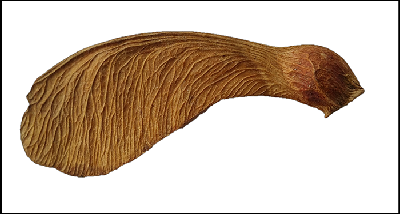
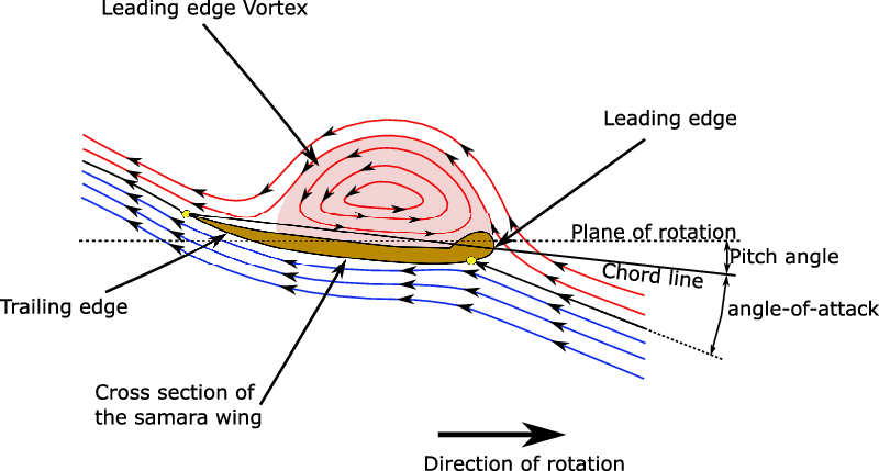
The samara seed is a generic type of winged tree-seed, like elm, maple, and ash (Fig. 1). The fibrous wing of the seed allows it to autorotate (self-spin) when separated from the tree branches, which in-turn will help to reduce its falling speed. This can enable the seed to be pushed further away from the parent tree for germination in the presence of wind(Reference Nathan, Katul, Horn, Thomas, Oren, Avissar, Pacala and Levin1). These seeds have been known to have very high sectional lift coefficients due to the development of what is known as a leading edge vortex (LEV) over the wing (Fig. 2). The LEV is a phenomenon whereby a vortex is developed along the wing from its leading edge. This LEV is an example of intricate flow mechanisms found to occur on natural wings such as with birds, insects, bats and samara seeds(Reference Lentink, Dickson, van Leeuwen and Dickinson2,Reference Salcedo, TreviÑo, Vargas and MartÍnez-SuÁstegui3) as well as on artificial delta wings(Reference Gursul, Wang and Vardaki4).
Some flying animals use flapping in order to generate and sustain LEVs leading to lower pressure (suction) and greater lift(Reference Shyy, Lian, Tang, Viieru and Liu5,Reference Shyy, Aono, Kang and Liu6) . It has also been suggested that a spanwise flow along the vortex core may be responsible for maintaining the stability of the LEVs(Reference Shyy, Lian, Tang, Viieru and Liu5). Furthermore, some insects, such as dragonflies, are able to configure their wing flapping motion in such a way that the LEV forms naturally and remains attached over the wing for the duration of the stroke(Reference Thomas, Taylor, Srygley, Nudds and Bomphrey7). Here the formation and shedding of the LEV is controlled by changing the wing angle-of-attack though, unlike samara seeds. Certain control of the creation of LEVs has also been seen in bats depending on their flight regime. For manoeuvring and slow flight, the increase in lift is useful, while the simultaneous increase in drag caused by the LEV is unlikely to be an issue due to the low flying speeds. However, the latter is not the case in cruising conditions, and therefore the bats, for example, are able to negate the creation of LEVs(Reference Muijres, Johansson, Winter and HedenstrÖm8).
Interestingly, such LEVs have also been observed in low aspect ratio (AR) delta wings. It has been found that the sweep angle is directly related to the relative contribution of vortex lift. Nonetheless, increased sweep angle also diminishes the angle-of-attack at which the vortices detach(Reference Gursul, Wang and Vardaki4).
Several experimental studies of samara LEVs have been performed successfully, obtaining good results and advancing the understanding in the topic. In 2009, Lentink et al. explained how different species of samara seeds use LEVs to improve their lift-generating characteristics during autorotation (self-spinning)(Reference Lentink, Dickson, van Leeuwen and Dickinson2). They also noted how more compact LEVs (due to decreasing angles of attack) and strong spanwise flows on the top of the aerofoil contributed to the attachment of the vortices and to better aerodynamic performance. Salcedo et al. later confirmed the importance of strong spanwise flow and strain produced by centrifugal forces in order to stabilise and attach the LEVs(Reference Salcedo, TreviÑo, Vargas and MartÍnez-SuÁstegui3). The attached LEVs create a straight cone pattern that augments lift generation and the spanwise flow stretches and adds intensity to the LEV, preventing its detachment.
Yasuda and Azuma(Reference Yasuda and Azuma9) on the other hand, concluded that the negative camber near the root, the pattern (surface roughness) of the fibrous wing and the leading-edge extra thickness close to the root, lead to the enhanced aerodynamic characteristics observed in samara seeds. Their work also suggested that the wing features of samara seeds may play a key role in the stability of their LEVs.
Example samara seed (Acer Pseudoplatanus – Sycamore) used in the experiments of this research.

Schematics of the samara LEV sectional streamlines.

Despite the above studies, it is remarkable that an adequate theoretical model, capable of describing and predicting the aerodynamic performance of samara seeds, even conceptually, is still lacking. Recently, Lee and Choi(Reference Lee and Choi10) suggested a scaling law to describe the relation between the lift force produced by a falling samara seed, its geometry, rotational speed and vertical descent speed. Their vortex-based theory predicted sectional lift coefficients, which agreed well with the presented numerical simulation as well as with data of 11 species of autorotating falling samara seeds. Furthermore, in Ansari et al.’s review on aerodynamic modelling of insect-like flapping flight(Reference Ansari, Żbikowski and Knowles11), several steady, quasi-steady and unsteady methods used to create different models were discussed, including techniques capable of modelling LEVs for insect flight and delta wings. It is expected that these theories can be extended to samara wings. In particular, a promising method was implemented inside Traub’s semi-empirical model (quasi-steady model with empirical corrections) in order to compute the effect of LEVs(Reference Traub12). This was Polhamus’ leading-edge suction analogy(Reference Polhamus13) originally developed for delta wings, but also used successfully in models for insect flight(Reference Traub12,Reference Nabawy and Crowther14) and lift generation of avian tails(Reference Maybury, Rayner and Couldrick15), among others. Polhamus’ model has been discussed along with LEVs by Nabawy(Reference Nabawy16), who suggested that LEVs increase the suction and thus the effective lift coefficient as well as increase the stall angle, thereby enlarging the flight envelope. Recently, Nabawy and Crowther(Reference Nabawy and Crowther17) studied the role of LEV in lift augmentation of steadily revolving wings, through investigating two hypotheses referred to as ‘additional lift’ and ‘absence of stall’. In this study, three different representations of the LEV lift were presented and analysed, building on previous work on quasi-steady lifting line model for insect-like hovering wings(Reference Nabawy and Crowther18). In this study, the normal force model achieved a better correlation with data in the literature than the Polhamus leading edge suction model or the trapped vortex model. These models can also be adapted to predict the performance of autorotating samara seeds.
In this paper, the authors present an adaptation of Polhamus’ method into an analytical expression capable of describing the sectional lift coefficient function for autorotating samara seeds. The developed lift coefficient expression is used within a numerical blade element model (BEM), which allows the performance of a falling autorotating seed to be predicted. Inherent assumptions are justified and the model is assessed against experimental wind tunnel data, corroborating its accuracy and applicability.
2.0 METHODOLOGY
This paper aims to develop a lift coefficient polar in function of angle-of-attack, which includes the effect of the LEV. This polar can subsequently be used in a blade element model to estimate the two-dimensional (2-D) lift force for the blade elements of the autorotating samara wing. Conventional blade element modelling approaches are widely used in the rotorcraft sector for estimating the performance of spinning rotor blades. These approaches are based on splitting the spinning blade into a finite number of 2-D wing elements and evaluating, for each element, the local flow characteristics, such as flow velocity components, Mach number, Reynolds number and angle-of-attack. The two-dimensional force and moment coefficient profiles for the relevant 2-D aerofoil sections can then be used to compute the local aerodynamic forces and moments acting on each blade element. Hence, the required aerodynamic forces and moments acting on the blade and eventually on the whole rotor can be computed by integrating these quantities across all the blade elements. Features such as unsteady aerodynamics, tip losses, etc. can also be included appropriately to increase the fidelity of the modelling. However, BEM calculations currently do not account for LEVs and as such require further adaptation to predict the aerodynamic performance of samara seeds.
Polhamus’ formulation will be used to produce the lift coefficient function with angle-of-attack for a finite idealised samara wing, which is assumed to create a LEV. This expression is subsequently used in a blade element model to estimate the local 2-D lift forces acting on each of the blade elements. This analysis assumes that the obtained lift coefficient polar from the Polhamus method, which is based on the finite 3-D wing, can be directly used to estimate the sectional 2-D lift coefficient for the blade element. This latter assumption was found to give good results, as will be shown later in the analysis. The validation of the Polhamus lift coefficient expression, within the BEM, was achieved through comparisons with other expressions of lift coefficient suggested by Azuma and Yasuda(Reference Azuma and Yasuda19) or based on the normal force model suggested by Nabawy and Crowther(Reference Nabawy and Crowther17). Furthermore, The BEM results were compared with experimental measurements obtained from testing natural samara seeds in a specifically designed vertical wind tunnel. In the following sections, the development of the LEV lift coefficient expression will be presented, followed by the description of the blade element code.
2.1 Development of analytical model for sectional LEV lift
Polhamus’ model(Reference Polhamus13) is based on an analysis of a finite wing using lifting surface methods to extract constants capable of describing the effect of the LEV on the total lift. It assumes that if the LEV remains attached over the upper surface of the wing, the total lift will be obtained as the sum of the potential lift and a vortex lift. This vortex lift is related to the suction force on the leading edge, translated as a normal force on the upper surface of the aerofoil by imposing a Kutta flow condition at the leading edge.
The justification for the use of Polhamus’ method for the samara wing comes from the extensions of Polhamus’ method found in literature. In Lamar’s application of the method for rectangular wings(Reference Lamar20), a side-edge suction force was shown to exist for this kind of wings, analogous to the leading-edge suction force. It was explained how vortex lift coming from the side-edge suction will tend to 0 as the aspect ratio AR (defined as the ratio between the span and chord of the wing) tends to infinity. Furthermore, in the data from Lamar published by Bradley et al. (Reference Bradley, Smith and Bhateley21), it can be seen how the side vortex lift reduces very steeply from AR = 0.5 to AR = 2, justifying the exclusion of side-edge vortex lift for the samara seeds considered hereafter, which have a typical AR of 4.38. Moreover, using an aerofoil with a non-sharp leading edge can be acceptable, as Lamar and Bradley et al. stated how a thicker leading edge would simply delay the creation of LEVs(Reference Lamar20,Reference Bradley, Smith and Bhateley21) .
The magnitude of the normal force at any wing section will be the same as the suction force created by the centrifugal force of the vortex lift. This can be expressed by potential flow and vortex lift components, in the following formulae (derived from Polhamus’ paper(Reference Polhamus13)).
2.1.1 Potential flow lift component
The potential lift coefficient  ${C_{L,p}}$
is given as
 \begin{align}{C_{L,p}} = {K_p}\sin \left( \alpha \right){\cos ^2}{\left( \alpha \right)}\nonumber\\[-20pt]\end{align}
where  $\alpha $
represents the local angle-of-attack and
 ${K_p}$
is a constant.
This potential flow lift coefficient  ${C_{l,p}}$
for small angles of attack will be reduced to
 \begin{align}{C_{L,p}} \approx {K_p}\alpha = {{\partial {C_{L,p}}} \over {\partial \alpha }}\alpha.\nonumber\\[-20pt]\end{align}
Therefore,  ${K_p}$
is obtained from the
 ${C_{L,p}}$
versus
 $\alpha $
curve adopting small angle theory and can be derived from any adequate lifting-surface theory. In this case, the vortex lattice method (VLM) code Tornado was used(Reference Melin22)Footnote 1. Once
 ${K_p}$
is found, it can be used in Equation (1) to calculate the potential lift
 ${C_{L,p}}$
for large angles. Given that Polhamus’ theory assumes a finite wing, the samara wing analysed in the lifting surface methods was simplified as a rectangular wing, with no sweep. Furthermore, the implementation of the VLM assumed that the wing will be subjected to a uniform flow velocity and did not consider the influence of rotation of the samara wing. In general, both the wing planform and flow velocity profile can affect the value of the lift curve slope
 ${K_p}$
as they are directly related to the aerodynamic lift. It would therefore be more accurate to account for them in the estimation of
 ${K_p}$
. Nevertheless, for a more complete analysis, the variation of the induced velocity and local angles of attack along the span of the wing also need to be considered, as well as the flow velocity profile and wing planform. These considerations greatly increase the model’s complexity, whereas the current authors envisage simplicity; this study tries to directly estimate and assess the 2-D lift coefficient function in which potential and vortex lift components are retrieved from the 3-D Polhamus lift theory based on a baseline rectangular wing subjected to a uniform flow velocity. The reader should be aware that methods that take into account these shortcomings in the estimation of the lift curve slope are available in the literature. A relevant example is the quasi-steady lifting line model suggested by Nabawy and Crowther(Reference Nabawy and Crowther18), who presented a novel approach capable of accurately estimating the aerodynamic forces from geometry and kinematics information alone.
The cross-sectional aerofoil shape of the samara wing is quite complex featuring low thickness overall, small camber, thickened leading edge and irregular surface texture, all of which were shown by Azuma and Yasuda(Reference Yasuda and Azuma9) to be important factors to reduce the descent speed of the autorotating seed. However, including the effects of all these features would required a more advanced analysis, which goes outside the scope of the current study. Instead, the NACA0005 aerofoil was selected for simplicity as it has low thickness to chord ratio (5%) and a leading edge with low radius of curvature, resembling the cross-section of the samara seed. In fact, the mean thickness to chord ratio of natural Acer Diabolicum Blume samaras was measured by Jung and Rezgui to be about 5%(Reference Jung and Rezgui23). Furthermore, it was found by Lentink et al. (Reference Lentink, Dickson, van Leeuwen and Dickinson2)Footnote 2 that the thickness to chord ratio of experimental artificial plate wings had to be equal to or below 4% to achieve a LEV similar to those seen by real samaras. The thickness of the leading edge was also shown by Yasuda and Azuma(Reference Yasuda and Azuma9) to be important in reducing the descent speed of artificial samaras, i.e. creation of a stronger LEV. Therefore, to account for the thickness of the seed as well as the thickness of the wing leading edge, the NACA0005 aerofoil was chosen in this study instead of a flat plate or other aerofoil alternative. This simplification was deemed acceptable in the present study, though a more comparative analysis of the effects of aerofoil shape on the performance of samaras is envisaged for future research.
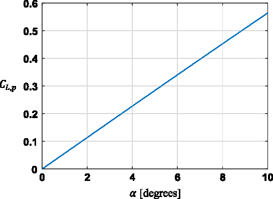
A range of wing aspect ratios (AR) was investigated but the chosen aspect ratio used in the rest of the analysis was 4.38, in accordance with typical values of samara seeds. The data were then used to obtain the required constants for Polhamus’ LEV lift, as discussed above. Therefore, the variation of  ${C_{L,p}}$
over angle-of-attack was obtained using a second-order accurate finite difference scheme (see Fig. 3).
CL,p over Angle of Attack curve obtained from VLM Tornado for the NACA0005 with AR = 4.38.

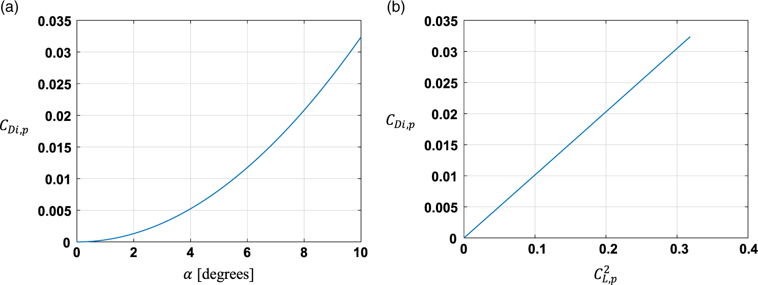
Variation of  $\textit{C}_{\textit{Di},\textit{p}}$
for NACA0005 from the VLM Tornado data. (a) Variation of
 $\textit{C}_{\textit{Di},\textit{p}}$
with angle-of-attack. (b) Variation of
 $\textit{C}_{\textit{Di},\textit{p}}$
with
 $\textit{C}_{\textit{L},\textit{p}}^2$
.

2.1.2 Vortex lift component
In the presence of a LEV, the suction force will be rotated into the direction normal to the wing chord plane. Once leading-edge thrust coefficient is determined, the vortex lift coefficient  ${C_{L,v}}$
can be evaluated as:
 \begin{align}{C_{L,v}} = {K_v}{{\cos\!\left( \alpha \right)} \over {\cos\!\left( {\rm{\Lambda }} \right)}}{\sin ^2}{\left( \alpha \right)}\end{align}
where  ${\rm{\Lambda }}$
is the sweep angle, assumed to be zero in the current application.
 ${K_v}$
is given by:
 \begin{align}{K_v} = ({K_p} - {K_p}^2{K_i})\end{align}
and  ${K_i}$
will be equal to:
 \begin{align}{K_i} = {{\partial {C_{Di,p}}} \over {\partial {C_{L,p}}^2}}\end{align}
where  ${C_{Di,p}}$
represents the induced drag coefficient and
 ${C_{L,p}}$
is the total lift coefficient. Both can be obtained from any reliable lifting-surface theory, such as VLM Tornado, similar to the analysis mentioned above for the potential lift component. In this analysis,
 ${K_i}$
was extracted using a second-order gradient scheme on the data set shown in Fig. 4. Finally, the total lift is given as the combination of the lift assuming potential flow and the lift induced by the vortex:
 \begin{align*}{C_L} = {C_{L,p}} + {C_{L,v}}\end{align*}
Hence:
 \begin{align}{C_L}\!\left( \alpha \right) = {K_p}\!\sin \left( \alpha \right){\cos ^2}{\left( \alpha \right)} + ({K_p} - {K_p}^2{K_i}){{\cos \left( \alpha \right)} \over {\cos \left( {\rm{\Lambda }} \right)}}{\sin ^2}{\left( \alpha \right)}\end{align}
Equation (6) can be used to evaluate the 2-D sectional lift coefficient. However, the exact estimation of the sectional lift for the samara seed is not necessarily straightforward because of the low Reynolds numbers and the changing complex aerofoil geometry along the span of the wing(Reference Azuma and Yasuda19). It will, therefore, be assumed that the 2-D lift coefficient expression will be applicable at any spanwise position of the wing. Furthermore, given the assumptions in the wing planform and velocity profile used in the VLM analysis, as discussed above, the 3-D lift coefficient expression in Equation (6) is first assumed in this study to be directly applicable to obtain the 2-D lift coefficients  ${C_l}\left( \alpha \right)$
, i.e.:
 \begin{align}{C_l}\!\left( \alpha \right) = {C_L}\!\left( \alpha \right) = {K_p}\sin\!\left( \alpha \right){\cos ^2}{\left( \alpha \right)} + ({K_p} - {K_p}^2{K_i}){{\cos \left( \alpha \right)} \over {\cos \left( {\rm{\Lambda }} \right)}}{\sin ^2}\left( \alpha \right)\end{align}
Methods to account for the three-dimensional (3-D) effects in correcting for the 2-D lift exist in literature. For example, Azuma and Okuno(Reference Azuma and Okuno24) used the local circulation method(Reference Azuma, Nasu and Hayashi25) to obtain sectional lift values from gliding flight test data of a pair of seeds of the Acer Diabolicum Blume. Seter and Rosen(Reference Seter and Rosen26) simply subtracted the induced angle-of-attack from the geometric angle-of-attack to obtain the 2-D lift. Here, the induced angle-of-attack  ${\alpha _i}$
is the consequence of the vortex field behind the finite wing and is given as
 ${\alpha _i} = \frac{{{C_L}}}{{\pi ARe}}$
, where
 ${C_L}$
is the lift coefficient of the finite wing with aspect ratio
 $AR$
, and
 $e$
is a geometric correction factor. Another method is to use the lift expression stemming from the Prandtl lifting-line theory(Reference Brandt, Stiles, Bertin and Whitford27), which can give good results for
 $AR$
above 3(Reference Schlichting and Truckenbrodt28). This method results in an explicit equation, which is usually used to evaluate 3-D lift for a wing given 2-D aerofoil characteristics, as it was used in(Reference Nabawy and Crowther29). However, this equation can be rearranged to obtain the sectional lift curve slope from the 3-D lift curve slope:
 \begin{align}{C_{l,\alpha }} = {{E{C_{L,\alpha }}} \over {1 - k{C_{L,\alpha }}/\left( {\pi AR} \right)}}\end{align}
 $E$
is the edge correction factor for the lifting line theory proposed by Jones(Reference Jones30) and
 $k$
is a correction factor to account for non-ideal non-uniform induced downwash. Both factors were assumed equal to 1 for simplicity. In order to get the value of
 ${C_l}\!\left( \alpha \right)$
from Equation (8), the fact that
 ${C_L}\!\left( \alpha \right)$
is proportional to
 $\sin \left( \alpha \right)\cos \left( \alpha \right)$
(see Equation (6)) can be used to obtain the value of
 ${C_{L,\alpha }}$
:
 \begin{align}{C_{L,\alpha}}\!\left( \alpha \right) = {{{C_L}\!\left( \alpha \right)} \over {\sin\!\left( \alpha \right)\cos\!{{\left( \alpha \right)}}}}\end{align}
Note that  ${C_{L,\alpha }}$
in Equation (9) contains the contribution of the Polhamus factor
 ${K_{Pol}}\left( \alpha \right)$
discussed by Nabawy and Crowther in(Reference Nabawy and Crowther17). Finally, the sectional 2-D lift coefficient can be obtained from Equation (8) using the same assumption in Equation (9), i.e.
 ${C_l}\left( \alpha \right)$
is also proportional to
 $\sin \left( \alpha \right)\cos \left( \alpha \right)$
, resulting in:
 \begin{align}{C_l}\!\left( \alpha \right) = {C_{l,\alpha }}\!\left( \alpha \right)\sin\!\left( \alpha \right)\cos\!{\left( \alpha \right)}\end{align}
Note that Equation (10) resembles the normal force model proposed by Nabawy and Crowther in(Reference Nabawy and Crowther17) but here the value of  ${C_{l,\alpha }}\left( \alpha \right)$
is a function of angle-of-attack.
2.2 Development of the blade element model
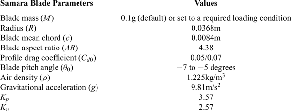
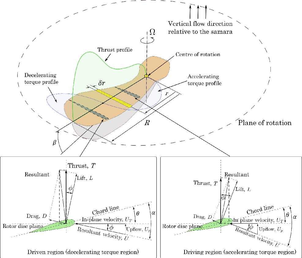
The previous section described the development of an analytical expression for the lift, capturing the effect of the LEV as a function of angle-of-attack. This expression was embedded in a simple numerical rotor model to analyse the aerodynamic performance of a falling samara seed in vertical autorotation. Figure 5 shows a representative schematic illustration of the modelled spinning samara seed and indicates the main flow and force components acting on it, as defined in the blade element code. The driving and driven torque regions present in the autorotation flight condition are also illustrated, together with their relevant flow and force vector structures. The rotor model is based on a blade element method (strip theory) using steady aerodynamics formulations combined with momentum theory. The blade element model (BEM) was coded in MATLAB as a set of algebraic equations describing the samara seed equilibrium condition in vertical autorotation descent, i.e. at terminal descent velocity. By numerically solving these equations the values of the rotational speed of the samara wing ( ${\rm{\Omega }}$
), its rate of descent (
 ${V_d}$
) and induced velocity (
 ${v_i}$
) could be extracted, for varying samara blade properties (see Table 1), such as rotor disk loading and blade pitch angle.
Blade properties used in the blade element model

The bold face was used to emphasise the numbers in percentages.
Schematic diagram illustrating the flow and force components acting on a samara wing, as defined in the blade element model. Angles are exaggerated for clarity.

In this analysis, the term “blade” is used to refer to the rotating samara wing, which is producing lift. The lift and drag forces acting on each blade element can be computed by first evaluating the local flow velocity components and angle-of-attack, as shown in Fig. 5. The tangential ( ${U_T}$
) and perpendicular (
 ${U_P}$
) components of the resultant velocity (
 $U$
) at a blade element located at a radial location (
 $r$
) can be expressed as:
 \begin{align}\left\{ \begin{array}{ll} {{U_T} = {\rm{\Omega }}r}\\[4pt] {{U_P} = ({{\rm{V}}_{\rm{d}}} - {v_i}){\rm{cos}}\,\,\left( \beta \right) - \dot \beta r}\end{array}\right. \end{align}
where  ${\rm{\Omega }}$
,
 ${v_i}$
,
 ${{\rm{V}}_{\rm{d}}}$
,
 $\beta $
and
 $\dot \beta $
are the rotational speed of the blade, the induced velocity at the blade element, the seed vertical descent speed, the blade flapping angle (coning) relative to the plane of rotation and the blade flapping rate respectively. The local angle-of-attack (
 $\alpha $
) is given by:
 \begin{align}\alpha = \theta + \phi \end{align}
where  $\theta $
is the elemental pitch angle and
 $\phi $
is the elemental inflow angle, which can be calculated as:
 \begin{align}\phi = {\rm{a\, tan}}\left( {{{{U_P}} \over {{U_T}}}} \right)\end{align}
The local elemental pitch angle  $\theta $
is a combination of the datum blade pitch angle (
 ${\theta _0}$
) relative to the plane of rotation (measured at 75% of the blade radius from the centre of rotation) and the local twist relative to the datum (
 ${\theta _t}$
), i.e.:
 \begin{align}\theta = {\theta _0} + {\theta _t}\end{align}
For simplicity, the local twist was ignored and hence  ${\theta _t}$
was considered equal to zero.
The elemental lift ( $\delta L$
) and drag (
 $\delta D$
) forces are calculated assuming two-dimensional steady flow as follows:
 \begin{align}\delta L = {1 \over 2}\rho {U^2}c\delta r{C_l}{\eta _{tip}}\end{align}
 \begin{align}\delta D = {1 \over 2}\rho {U^2}c\delta r{C_d}\end{align}
where  $\rho $
,
 $c$
and
 $\delta r$
are the air density, blade local chord and blade radial elemental width respectively. Note that because the local angle-of-attack varies along the spanwise direction, the local lift coefficient,
 ${C_l}$
, will also vary radially. This change is captured by Equations (7) or (10). The parameter
 ${\eta _{tip}}$
is a tip loss influence factor adapted from Leishman(Reference Leishman31):
 \begin{align*}{\eta _{tip}} = {2 \over \pi }{\rm{a\, cos}}\,{e^{ - f}},\,{\rm{where }}\ f = {1 \over 2}\left( {{{1 - {r \over R}} \over {{r \over R}\phi }}} \right)\end{align*}
and  $R$
is the blade radius.
The local drag coefficient is symbolised by  ${C_d}$
, which can also be a function of angle-of-attack but was taken as a constant at first in this analysis, i.e.
 ${C_d} = {C_{d0}}$
. Typical values for
 ${C_{d0}}$
were quoted by Azuma and Yasuda for the Acer Diabolicum Blume samara to be between 0.05 and 0.07(Reference Azuma and Yasuda19). The assumption of constant
 ${C_d}$
is often used in basic helicopter performance models since the angles of attack are relatively small for most of the blade span. For the autorotating samara however, the angles of attack are substantially larger and hence an appropriate sectional drag polar is needed. Since the blade drag strongly influences the torque balance in autorotation, the accurate estimation of the samara rotational speed is, therefore, dependent on how representable the drag equation is in the numerical model. In this analysis, three expressions for the sectional drag coefficient were considered:
 \begin{align}{C_d} = {C_{d0}}\end{align}
 \begin{align}{C_d} = {C_{d0}} + {C_l}\tan \left( \alpha \right)\end{align}
 \begin{align}{C_d} = {C_{d0}} - 0.008\alpha + 4.27{\alpha ^2} - 2.50{\alpha ^3}\end{align}
While the first drag expression (Equation (17)) only considers the profile drag coefficient, which is assumed constant, the other two equations take into account the induced drag contribution as well. Equation (18) was discussed by Nabawy and Crowther(Reference Nabawy and Crowther17) to give a satisfactory drag coefficient representation for revolving wings, operating at moderate to high angles of attack. On the other hand, Equation (19) was proposed by Azuma and Yasuda(Reference Azuma and Yasuda19).
The elemental thrust force  $\delta T$
and torque
 $\delta Q$
can be evaluated by respectively projecting the lift and drag force vectors vertically and horizontally (Fig. 5), yielding
 \begin{align}\delta T = \delta L\cos \left( \phi \right) + \delta D\sin \left( \phi \right)\end{align}
 \begin{align}\delta Q = \left( {\delta L\sin \left( \phi \right) - \delta D\cos \left( \phi \right)} \right)r\end{align}
The total thrust force and aerodynamic torque acting on the blade are finally calculated by summing all elemental contributions from the root to the tip of the blade, i.e.
 \begin{align}T = \mathop \sum \nolimits_{i = 1}^n \delta T\cos (\beta )\end{align}
 \begin{align}Q = \sum\nolimits_{i = 1}^n {\delta Q} \end{align}
where  $n$
and
 $i$
are the number and the index of the blade elements respectively.
Following(Reference Leishman31) the thrust predicted from the momentum analysis ( ${T_m}$
) can be extracted as
 \begin{align}{T_m} = 2\rho A\left( {{V_d} - {v_i}} \right){v_i}\end{align}
where  $A = \pi {R^2}$
is the rotor disc area and
 $R$
is the rotor radius. This momentum equation gives reasonable estimation of the thrust and/or the induced velocity. Here, the induced velocity
 ${v_i}$
is assumed constant across the rotor disc, or in the case of the samara seed, across the samara wing.
Finally, in a steady state descent of the autorotating seed the following algebraic expression can be used to describe the equilibrium condition:
 \begin{align}\left\{ \begin{array}{ll}{T\cos \beta - {T_m} = 0}\\[4pt] {T\cos \beta - Mg = 0} \\[4pt] {Q = 0}\end{array} \right.\end{align}
M, g are the blade mass and gravitational acceleration respectively. Solving the above algebraic equations numerically results in predicting values for  ${v_i}$
,
 ${V_d}$
and
 ${\rm{\Omega }}$
for a given set of blade parameters. The equations were coded in MATLAB and the numerical function “
 $\textsf{fsolve.m}$
” was used to solve the algebraic expressions in Equation (25).
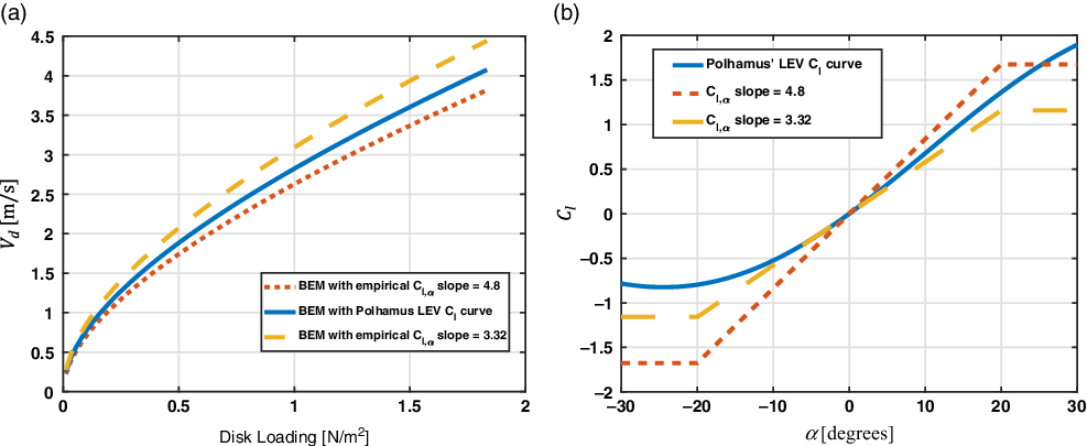
Initially, three different lift coefficient functions were adopted in the BEM: the analytical function introduced in this work (developed using Polhamus’ analogy as shown in Equation (7)) and two other empirical lift curves suggested by Azuma and Yasuda(Reference Azuma and Yasuda19). Figure 6(b) corroborates the lift curve obtained from the analytical LEV model to be sensible, falling between the range of the minimal and maximal experimental values obtained by Azuma and Yasuda(Reference Azuma and Yasuda19), for  ${\rm{\alpha }}$
between 0 and 25 degrees. The predicted descent speed of the autorotating seed is shown in Fig. 6(a) for the three different lift curve functions. The curves follow the expected theoretical trend as discussed in(Reference Azuma and Yasuda19) where in this case, the descent speed curve predicted using the Polhamus’ method is bounded by the other two curves.
Variation of the samara seed vertical descent speed ( $\textit{V}_{\textit{d}}$
) with disk loading calculated as
 $\textit{Mg}/(\textit{pi}*\textit{R}^{\text{2}})$
(a) for different lift coefficient functions (b). The
 $\textit{C}_{\textit{l}}$
curves were obtained from Polhamus’ method using AR = 4.38 and from experimental tests from Azuma and Yasuda(Reference Azuma and Yasuda19) with a “stall” (plateau) at
 $\alpha $
= ±20 degrees.

Three other models of the lift coefficient were also adopted in the BEM: the developed Polhamus model but with the 2-D corrections as expressed in Equations (8)–(10) and two models based on the normal force analogy given as:
 \begin{align}{C_l}\left( \alpha \right) = {C_{l,\alpha }}\sin \left( \alpha \right)\cos {\left( \alpha \right)}.\end{align}
Unless already known, values of  ${C_{l,\alpha }}$
can be obtained in a similar fashion as implemented in Equations (8)–(10) if the value of the 3-D lift curve slope is known. However, for simplicity
 ${C_{l,\alpha }}$
is given the same values used in the Azuma and Yasuda lift model, i.e.
 ${C_{l,\alpha }} = $
3.32 or 4.8.
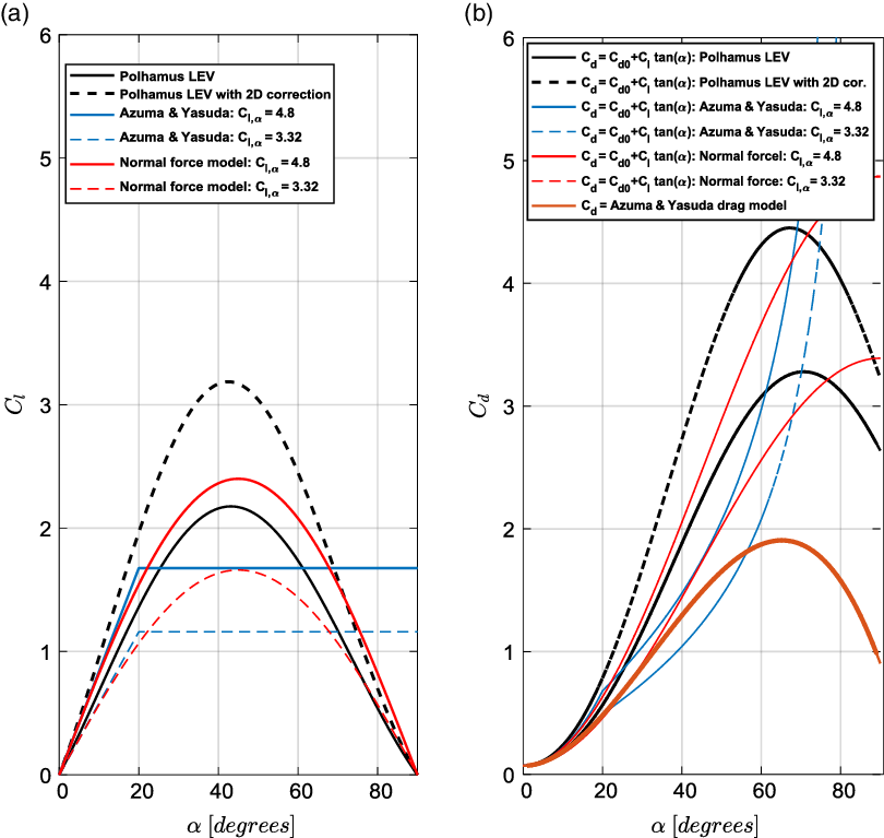
A comparison of all the lift coefficient profiles used in this study is shown in Fig. 7(a), for a range of angles of attack from 0 to 90 degrees. The corresponding drag plots based on Equation (18) are also shown in Fig. 7(b). For comparison, the drag equation suggested by Azuma and Yasuda, described by Equation (19) is also plotted. The drag coefficients expressed by Equation (18) can be noted to attain substantially large to unrealistic values for high angles of attack. The use of such drag plots will have a detrimental effect on the estimation of the correct rotor speed using the BEM. Therefore, it was decided to only consider the drag plot suggested by Azuma and Yasuda, i.e. by Equation (19) given that the resulting profile looks more reasonable.
Comparison of different lift models used with the corresponding drag plots. (a) Lift coefficient, (b) drag coefficient.

Figure 7(a) also shows that the 2-D correction applied to the lift coefficient expressed by the Polhamus analogy increases its values. For example,  ${C_l}$
increased by about 47% at
 $\alpha \approx 45$
, leading to the highest
 ${C_{l,max}}$
compared with other models.
2.3 Wind tunnel experiments
To validate the results of the developed BEM with the sectional lift model, experiments of autorotating natural samara seeds were carried out in a vertical, low-speed wind tunnel. The wind-tunnel testing allowed the validation of the model at a range of vertical wind speeds and not only at the natural terminal velocity of the seeds. On the other hand, basic validation of the BEM without Polhamus-based lift model was previously performed by Jung and Rezgui(Reference Jung and Rezgui23) using drop tests (free fall) data of natural seeds.
A number of experimental studies on the flight dynamics and aerodynamics of samara seeds have been reported in literature (e.g.(Reference Lentink, Dickson, van Leeuwen and Dickinson2,Reference Salcedo, TreviÑo, Vargas and MartÍnez-SuÁstegui3,Reference Lee, Lee and Sohn32,Reference Limacher and Rival33) ). These studies were carefully analysed to obtain a good insight into the construction of the proper experimental setup for the purpose of achieving the objectives of this validation study. This phase of research was concluded by designing and building a specific vertical low speed tunnel.
2.3.1 Description of the vertical wind tunnel
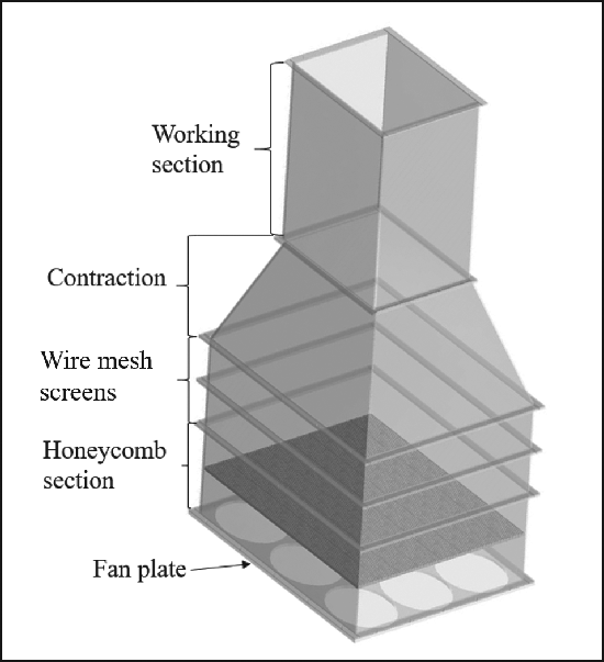
The main design requirement for the tunnel was to provide an adequately uniform flow of approximately 0.5m/s to 2m/s at the working section with tunnel height constrained to 2.5m. The wind tunnel was designed to be modular such that future modifications and improvements could be easily accommodated. The tunnel wall panels were made from acrylic glass, with reinforcements in the corners to ensure the rigidly of the structure. The transparent acrylic glass facilitated the observation of the experiments and would allow future Particle Image Velocimetry (PIV) measurements to be performed. From basic wind tunnel design guidelines(Reference Bradshaw and Pankhurst34,Reference Brusca, Lanzafame and Messina35) , several sections for the wind tunnel were identified (Fig. 8): working section, contraction, two wire mesh turbulence-reduction screens, honeycomb screen, and fan section (or in this case, a fan plate). A provision for a diffuser was also considered.
Schematic of the designed low-speed vertical wind tunnel with its different modules.

The working section was designed with internal dimensions of 340mm × 340mm, and a total length of 600mm. The contraction section, with a contraction ratio of 3.06, connected the top wire-mesh-panel sections with the working section. Furthermore, a 20mm thick honeycomb mesh, positioned 100mm away from the fans, was used to reduce flow swirl. To further reduce turbulence eddies and decrease the spatial flow non-uniformity after the honeycomb screen, the mesh pitch and wire diameter for the two wire-mesh screens were chosen to be 1.27mm and 0.25mm respectively. The two screens were positioned 150mm apart (> 500×wire diameter), as suggested by Bradshaw and Pankhurst(Reference Bradshaw and Pankhurst34).
The fan plate was attached to support a total of nine fans delivering the air flow into the working section. To this extent, nine BitFenix Spectre PRO fans (230mm in diameter each)(36) were used to generate the required flow speeds in the wind tunnel. The fans were connected on a parallel circuit to a power source capable of regulating the voltage delivered to the circuit, allowing the wind speed to be controlled. Further details about the wind tunnel design are described by the authors in(Reference Arroyo, Rezgui and Theunissen37).
2.3.2 Wind tunnel characterisation
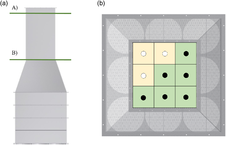
To carry out a basic flow characterisation process, two anemometers and a mini-CTA (Constant Temperature Anemometer) probe(38) were used to perform wind speed measurements at the end of the contraction section (the point of connection between the contraction and the working section) and at the end of the working section (see Fig. 9). It is worth noting that the anemometers had a precision of 0.1m/s, while the mini-CTA probe could measure variations of 0.001m/s. After checking the correct calibration of the probe, its measured wind speed was compared with the values from the anemometers, to ensure that the latter were also correctly calibrated.
Front (a) and top (b) view of the characterisation measurements. (a) Horizontal planes of measurement for the wind tunnel characterisation: A) Plane at the end of the working section, B) plane at the connection between the contraction and the working section. (b) Points of wind speed measurement on the horizontal measurement planes. Green cells show the wind speeds directly obtained by measurements; yellow cells show the ones calculated by symmetry.

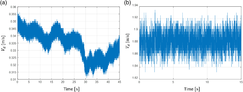
Given that the mini-CTA allowed to record measurements during lapses of time, it was used to observe the steadiness of the flow at different voltage-current inputs of the wind tunnel. In Fig. 10(b), it can be seen that the flow was relatively steady for the 12V setting, with small fluctuations in the flow vertical velocity ( ${V_d}$
) in the order of 0.08m/s (4.3%). For the 3.9V setting, the flow was much more unsteady, with changes in velocity of at most 0.045m/s (~12%), see Fig. 10(a). This was observed to take place because the electrical current was not enough to power all fans, causing some fans to work intermittently. The highly unsteady and fluctuating flow (~12%) was only observed for the 3.9V setting. All tests were however performed at higher voltage inputs (4V or higher) for which the flow was found to be as steady as in the case shown in Fig. 10(b).
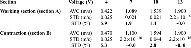
Characterisation of tunnel vertical velocity ( ${\textit{\textbf{V}}}_{\textit{\textbf{d}}}$
) measured at the different points at each of sections A and B: average (AVG) and standard deviation (STD) from nine measurement points

Having selected and calibrated the anemometer, measurements in the wind tunnel were performed to check for flow uniformity across the working section. As observed in Fig. 9, these were performed at two streamwise locations of the wind tunnel: just before the exit of the working section (plane A in Fig. 9) and the intersection between the contraction and the working section (plane B in Fig. 9). The measurements at plane B were taken without the working section present. The speed measurements were obtained at six points of each plane, which, after considering the symmetry of the structure, were translated into nine measurements (in Fig. 9(b), the points directly measured are marked by black solid circles, whereas the measurements calculated by symmetry are shown as hollow circles). Since the purpose of the tests was to measure and characterise the flow at the middle (central area) of the working section, a course test grid was deemed adequate. A full survey of the flow quality of the tunnel will be considered in the future.
The measurements were taken at settings in which the flow was quasi-steady, to observe its uniformity. Accordingly, fan input voltages above 3.9V were considered: 4V, 7V, 10V and 13V. The average and standard deviation of the values are documented in Table 2. From these measurements it was concluded that for a voltage range between 4V and 13V, the wind tunnel produced a near-steady and uniform flow across the two planes A and B (Table 2). In particular, the standard deviation (STD) was below 2% in the working section for voltages above 7V. Furthermore, there was almost no variation in speed (STD approx. 0%) across the nine locations in some voltage settings. These cases were attributed to the low resolution of 0.1m/s of the anemometers used combined with the low fluctuation in the average flow speeds.
2.3.3 Samara seed preparation
Several samples of sycamore seeds (Acer Pseudoplatanus)(39,40) were collected in autumn and kept in a sealed container. Humidity levels were checked daily to ensure preservation of the specimens. The criteria for selecting the seeds was the health of the seed, the span of the wing and the aspect ratio (as suggested by Yasuda and Azuma(Reference Yasuda and Azuma9)). The best two specimens fitting the criteria were selected and prepared for the experiments. This involved calculating their centre of gravity position (CG) in order to find their natural centre of rotation and hence minimise potential imbalance induced vibrations that could disturb the experiments. Both seeds had an aspect ratio of approximately 4.38, which defined the variables in the simulations pertaining to Polhamus’ analogy reported in Section 2.1.
At the approximate CG, a hole was drilled in the seed with a 0.5mm straight needle. The seed was positioned in the centre of the working section of the wind tunnel using 0.23mm thin fishing wire, which was inserted at the CG position of the seed through the hole. Two knots in the fishing wire with 2mm beads were added above and below the seed to restrict it from moving vertically. The beads were used to minimise friction and possible jamming of the knots in the holes of the seeds. The fishing wire was attached to the tunnel through two other sets of fishing wires, which were tightly connected diagonally and horizontally between the corners of the working section at the top and bottom of the working section.
Mini-CTA probe vertical flow speed measurements at the centre of the top end of the wind tunnel working section. (a) measurements at fans’ voltage of 3.9V (current = 0.8A) and (b) measurements at fans’ voltage 12V (current = 2.8A).

3.0 EXPERIMENTAL MEASUREMENTS
The experimental tests were performed for the analytical model validation by measuring the rotational speed ( ${\rm{\Omega }}$
) at different vertical flow velocities (
 ${V_d}$
). Videos recorded by a Photron Fastcam SA1.1 high-speed camera were used to obtain the rotational speed of the samara wing. The video recordings were made at 15,000 frames per second, which gave an error of less than 1.4rpm for the slowest rotational speed recorded (~550rpm) and less than 21.5rpm for the highest (~2600rpm). The error in determining the rotor speed was due to the achieved precision of approximately three frames in matching the seed azimuth angle after one rotation, which was done manually on a frame by frame basis. The vertical flow velocity (
 ${V_d}$
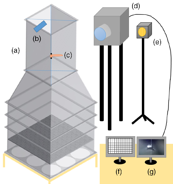
) was given by the wind tunnel speed, measured by an anemometer positioned at the end of the working section, in one of the outer points of section A in Fig. 9 (see Fig. 11). The presence of the spinning samara seed in the working section did not have a noticeable effect on the flow speed with respect to the vertical position where the measurements were taken. Therefore, any errors in flow speed because of the positioning the anemometer downstream of the spinning seed were deemed acceptable, given the resolution of the anemometer. To reduce human error and to check for any hysteresis behaviour, the seed rotational speed measurements were performed twice. First, by changing the voltage from lowest to highest setting and then from highest to lowest. These measurements were repeated twice.
Schematic of the final experimental set up, including: A) Wind tunnel, B) anemometer for wind speed measurements, C) sample samara seed, D) high speed camera for rotation observation, E) LED spotlight, F) computer for measurements input, G) computer receiving high speed camera video.

The voltage settings used to regulate the wind tunnel speed ranged from 4V (~0.42m/s) to 13V (~1.9m/s) with steps of 0.5V. Each wind speed measurement was averaged over 15 seconds to take into account any short-term variations in the initial value.
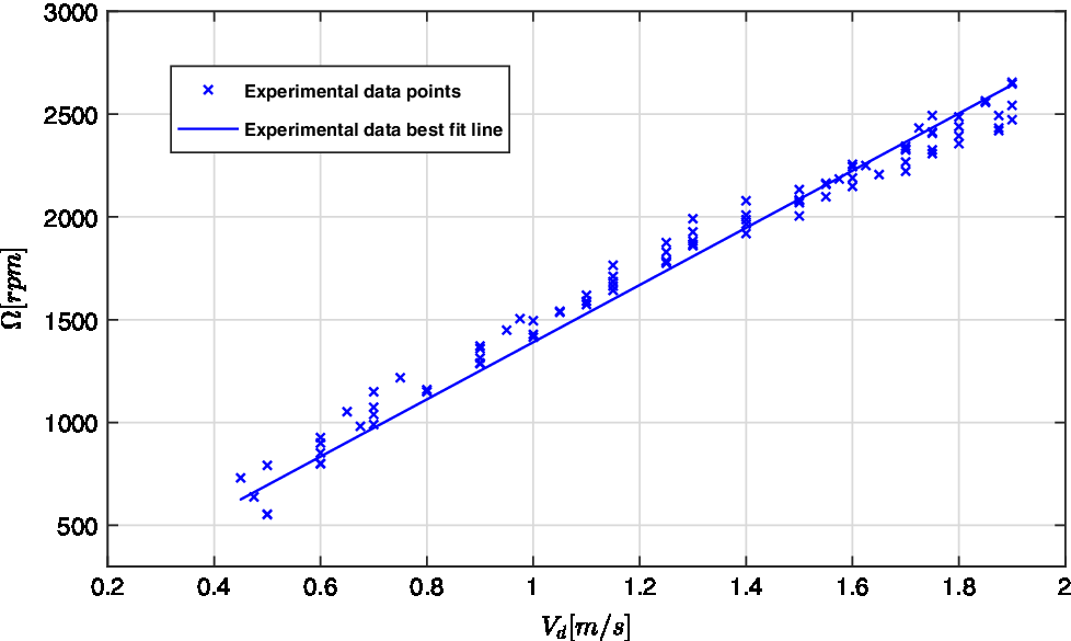
Figure 12 shows a plot of the measured rotational speed values against vertical flow speed ( ${V_d}$
) values. The line of best fit passing through the origin (0, 0) is also illustrated. Furthermore, the high-speed camera was used to measure the coning and pitch angles. It is worth noting that due to the nature of the experiments and the preparation of the samples (with the axis of rotation drilled through the CG, and the fishing wire parallel to the air flow) the coning and pitch angles were quite restricted.
Experimental measurements (solid dots) for samara seed rotational versus wind speed, with best fit line (blue solid line).

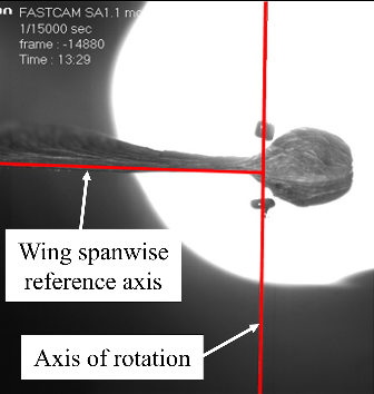
From the coning angle measurements (see example in Fig. 13), it was observed that the coning angle was close to 0 degrees for the whole speed range. The coning angle in the free fall condition is generally higher than 0 degrees though. It was thus clear that the vertical wire restricted the coning angle in the wind tunnel setup, though this would not hinder the results of this analysis. By visual inspection of the video footages of the seed at selected azimuth angles, no evident cyclic blade flapping behaviour was observed and hence the flapping rate of the seed was taken to be zero. The pitch angle measurement presented more difficulty due to the natural twist of the blade and the imprecise definition of the chord line. Nevertheless, by inspection from the still images of the high-speed camera recordings in a similar fashion as was done for the estimating the blade coning, the blade pitch angle was estimated to be between −5 and −7 degrees relative to the plane of rotation. These measurements were used accordingly in the BEM analyses. Note that the fact the seed was tethered to the fishing wire meant it was not allowed to autorotate at its natural blade pitch angle or coning angle.
Coning angle measurements using the high-speed camera at  $\textit{V}_{\textit{d}} \approx $
1.9m/s (13V).

4.0 NUMERICAL ANALYSIS
The blade element model presented in Section 2.2, fitted with the analytical LEV expression for  ${C_l}$
, was updated with the parameter values obtained from the experiment. The wing coning angle and the flapping rate were set to 0deg and 0rad/s respectively, whereas the pitch angle was varied between −5 and −7 degrees.
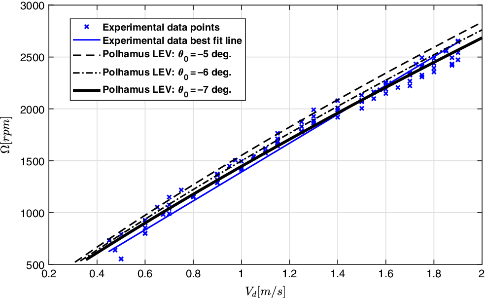
The numerically-predicted variation of rotational speed versus vertical flow speed for blade pitch angles of −5, −6 and −7 degrees are compared in Fig. 14 with the data measured for the natural samara seed in the vertical wind tunnel. In this case, the lift coefficient function in Equation (7) was used and the drag coefficient  ${C_d} = {C_{d0}} = 0.07$
was used. The prediction from the blade element model shows a good agreement with the experimental measurements; the best fit curve of the experimental data almost overlaps the curve from the analytical LEV model for a pitch angle of −7 degrees (Fig. 14). These results illustrate a good agreement in both trend and values of rotational speed over wind speed and hence confirms that the analytical model for leading edge vortex lift developed from Polhamus formulations is valid for estimating the performance of autorotating samara seeds in vertical descent. The results also show that the blade element modelling approach is adequate in predicting the rotor speed of autorotating samara seeds despite the basic drag representation.
Variation of samara seed rotational speed ( $\mathrm{\Omega} $
) with vertical flow speed (
 $\textit{V}_{\textit{d}}$
) from the experimental wind tunnel results and the tuned BEM (for three blade pitch angles),
 $\textit{C}_{\textit{d}} = \textit{C}_{\textit{d}0} \text{0}\, \textit{=}\, \text{0.07}$
.

Next, multiple runs by the BEM were performed for the pitch angle  ${\theta _0} = - 7$
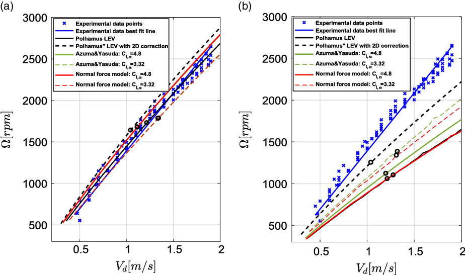
degrees but in this case, all the different expressions of the sectional lift coefficient were tested. The comparison is shown in Fig. 15(a). Surprisingly, all lift cases seem to give adequate predictions of the variation of rotor speed versus flow speed when compared with the experimental data, with a slight over prediction of the rotational speed by the Polamus lift model with the 2-D corection. The normal force and Azuma and Yasuda lift models seem to produce almost identical curves. Furthermore, although the results illustrated yet another argument in favour of using the developed Polhamus’s model to capture the LEV lift effect, the analysis assumed a constant drag coefficient value of
 $0.07$
. These favorable results diminish when the drag plot suggested by Azuma and Yasuda (Equation (19)) is used instead, see Fig. 15(b). Both the Polhamus LEV model and normal force model with
 ${C_{l,\alpha }} = 4.8$
have the biggest discrepancy relative to the experimental data, with the Polhamus model with the 2-D corrections achieving the lowest difference.
Variation of samara seed rotational speed ( $\Omega $
) with vertical flow speed (
 $\textit{Vd}$
) from the experimental wind tunnel tests and the BEM, for
 $\theta_{0}\, \text{=}\, - \text{7}\textit{deg}$
. (a)
 $\textit{C}_{\textit{d}}\, \text{=}\, \textit{C}_{\textit{d}\text{0}}\, \text{=}\, \text{0.07}$
and (b)
 $\textit{C}_{\textit{d}}\, \text{=}\, \text{0.07} - \text{0.008}\alpha \text{+}\, \text{4.27}\alpha \text{2} - \text{2.50}\alpha \text{3}$
. Black hollow circles indicate points at which the thrust generated by the autorotating samara is equal to the weight of the natural seed.

The results in Fig. 15(b) indicate the drag effects on the prediction of the seed performance. These results were expected since drag plays a big role in the torque balance in autorotation, which greatly affects the rotational speed in steady state. Moreover, because of the large angles of attack, or more precisely, the inflow angles, the drag can also moderately contribute to the overall thrust produced by the spinning seed. This will eventually have an effect on the descent speed of the seed. The torque and the thrust-weight balance of the falling autorotating seed is quite complex and is shown in Fig. 15 to be very sensitive to sectional lift and drag characteristics. To further appreciate this argument, Fig. 15 indicates the points — shown by black hollow circles — at which the thrust generated by the autorotating seed is equal to the weight of the natural samara seed. It can be seen that while the vertical descent speed reduces with the lifting capability of the seed (high  ${C_l}$
profiles, see Fig. 7), for the case of constant drag coeffcient (Fig. 15(a)), the points seem to scatter in a random way when the drag plot suggested by Azuma and Yasuda (Equation (19)) is used (Fig. 15(b)).
To further scrutinise the effects of the drag, the profile and induced drag components were separately assessed. In both cases, Equation 19 was used for the drag representation. In the first case, a value of 0.05 instead of 0.07 was used for  ${C_{d0}}$
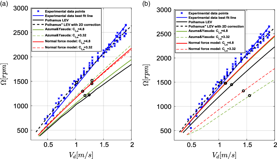
. The new value was also suggested by Azuma and Yasuda(Reference Azuma and Yasuda19) for Acer Diabolicum Blume seed. In the second case, the induced drag contribution as per Equation (19) was reduced by 50% for simplicity. The BEM results are shown in Fig. 16. It can be seen that the Polhamus LEV model with the 2-D corrections achieved a very good match with the experimental data, for both drag cases. However, the results of the other models seem to vary rather arbitrarily depending on the interplay of the aerodynamics forces acting on the autorotating seed to achieve the torque and weight equilibrium. For example, for the normal force and Azuma and Yasuda models with
 ${C_{l,\alpha }} = 3.32$
, the descent speed is generally higher in Fig. 16(b) relative to Fig. 15(b). This case indcates that the induced drag was greatly contributing to the overall thrust generated by the rotating seed. In general, the results obtained in this study are promising and shows the importance of having good sectional lift and drag models for the accurate prediction of the performace of autorotating samara seeds.
Variation of samara seed rotational speed ( $\Omega $
) with vertical flow speed (
 $Vd$
) from the experimental wind tunnel tests and the BEM, for
 $\theta_{\text{0}} = - 7deg$
. (a)
 $\textit{C}_{\textit{d}} = 0.05 - 0.008\alpha + 4.27\alpha 2 - 2.50\alpha 3$
and (b)
 $\textit{C}_{\textit{d}} = 0.07 + 0.5\left( { - 0.008\alpha + 4.27\alpha 2 - 2.50\alpha 3} \right)$
. Black hollow circles indicate points at which the thrust generated by the autorotating samara is equal to the weight of the natural seed.

5.0 CONCLUSIONS
An analytical model capable of modelling the sectional lift on a samara seed experiencing a leading edge vortex (LEV) was developed and validated. The formulation used Polhamus’ leading-edge suction analogy for LEV lift for 3-D finite wings for a given wing aspect ratio and was adapted to produce two analytical 2-D lift coefficient expressions for rotating wings as a function of angle-of-attack. These lift coefficient expressions were incorporated into a blade element model (BEM) in estimating the sectional lift force to simulate the performance of a falling and autorotating samara seed. Furthermore, wind tunnel tests were conducted using a specifically designed and constructed vertical wind tunnel facility. The experiment allowed the rotational speed of autorotating samara seeds to be measured for different flow speeds.
The BEM was updated with the coning angle and pitch angles measured during the wind tunnel tests. The results from the experiments were compared against those predicted by the numerical model, showing good agreement of the Polhamus LEV model for cases when the drag coefficient was taken as constant along the seed wing span. The results were also compared with numerical predictions using the BEM but using different lift coefficient expressions available in the literature. For cases, where induced drag contributions were acounted for, the Polhamus LEV with 2-D corrections achieved the best match with the experimental test data. In summary, it was shown that an analytical model capable of predicting the sectional lift on a rotating samara wing with an active LEV was developed, using an adaptation of Polhamus’ analogy.
Despite the successful analysis, additional validation studies are desirable to further assess the validity of the analytical lift model and the BEM at different flight conditions, particularly at different settings of blade pitch and coning angles. With the creation and validation of a numerical model, which can predict the rotational speed and vertical rate of descent of falling samara seeds, another step was taken towards the understanding of LEVs over samara seeds and towards their use in the design of more efficient rotors and micro rotary vehicles. Future work will also focus on enhancing the experimental setup to allow for thrust measurements and to further validate the numerical model at different parameters.
6.0 DATA ACCESS STATEMENT
All underlying data are provided in full within this paper.