INTRODUCTION
Numerous authors have suggested that local population densities should be highest in the core (centre) of their geographic range, and decline in density toward the periphery (edge) of the range. Hengeveld & Haeck (Reference HENGEVELD and HAECK1982) suggested that the trend was sufficiently robust across a broad range of organisms to be labelled a general biogeographical rule. Subsequent studies continued to find support for the trend (Brown et al. Reference BROWN, MEHLMAN and STEVENS1995).
The centre–edge gradient in local density (hereafter referred to as the ‘centre–edge gradient’) has been attributed to habitat becoming less favourable from the centre to the edge of the range of a species. A number of theoretical models have been developed to explain the possible mechanisms for this gradient (Brown Reference BROWN1984, Guo et al. Reference GUO, TAPER, SCHOENBERGER and BRANDLE2005, Maurer & Brown Reference MAURER and BROWN1989, Williams Reference WILLIAMS1988). Nevertheless, not only have a substantial number of studies reported data inconsistent with the centre–edge gradient, but only a minority of studies reporting the gradient sampled the whole of the geographic range of the species (Sagarin & Gaines Reference SAGARIN and GAINES2002).
The existence of the gradient and related explanations have broad theoretical and practical implications. These explanations underlie hypotheses arguing why dynamics of edge populations might be more variable than those of centre populations, why edge populations might be more prone to extinction, why edge populations may be more resistant to climate change, and why reintroduced species might do better at the historical centres of their range (Sagarin & Gaines Reference SAGARIN and GAINES2002).
The centre–edge gradient has typically been studied in plants, insects and birds, with very few studies on mammals. For instance, only one of the 22 empirical studies reviewed by Sagarin & Gaines (Reference SAGARIN and GAINES2002) addressed mammal species. There is also a distinct lack in the literature on the centre–edge gradient of studies of tropical taxa: all of the 22 studies reviewed by Sagarin & Gaines (Reference SAGARIN and GAINES2002) were of temperate taxa, and 20 of these reported on Western European and North American taxa. This temperate bias is true of macro-ecology in general, despite the greater biodiversity of the tropics (Gaston & Blackburn Reference GASTON and BLACKBURN1999, Harcourt Reference HARCOURT2006, Janzen Reference JANZEN1986). If tropical taxa behave differently from temperate taxa (Cardillo Reference CARDILLO2002, Ghalambor & Martin Reference GHALAMBOR and MARTIN2001, Turner & Hawkins Reference TURNER, HAWKINS, Lomolino and Heaney2004), observations from well-studied temperate biotas cannot be extrapolated to the less well-studied tropics.
The relative lack of knowledge of the tropics is particularly dire for tropical forest mammals, with the exception of the primates. We know an extraordinary amount about a relatively large proportion of primate species (Campbell et al. Reference CAMPBELL, FUENTES, MACKINNON, PANGER and BEARDER2007, Fleagle et al. Reference FLEAGLE, JANSON and REED1999). Therefore, in this study, we use primates as exemplars of tropical forest mammals. Macro-ecological analysis across only part of the geographic range of a species can produce different results from analysis across the whole range (Gaston et al. Reference GASTON, BLACKBURN and LAWTON1997). We obviate this potential problem by identifying centre and edge in relation to each species' entire geographic range. We do not predict a decline from centre to edge, because of the inconclusiveness of previous studies of the gradient.
Unlike most studies of centre–edge gradients, we account for environmental quality in our study by taking account of the level of disturbance reported at the study sites. Although some primate species do well in disturbed secondary forests, most do not (Fimbel Reference FIMBEL1994, Harcourt Reference HARCOURT and Caro1998, Johns & Skorupa Reference JOHNS and SKORUPA1987, Plumptre & Reynolds Reference PLUMPTRE and REYNOLDS1994, Skorupa Reference SKORUPA and Benirschke1986). We therefore predict that population densities will usually be lower in more disturbed habitat, irrespective of position in the geographic range.
METHODS
Data sources
All data for density and level of disturbance were extracted from the primary literature. For all statistical analyses, we used data from only those sites where densities had been recorded for ≥ 3 mo. Sources for geographic ranges of species and genera are presented in Harcourt (Reference HARCOURT2000). The geographic range for a genus was determined as the outline of the superimposed ranges of all species within that genus.
We recorded density as individuals km−2, converting to this measure from whatever measure the original authors reported, for example multiplying group size by number of groups km−2 if those were the measures reported. When a minimum–maximum range of densities for a species in a single site was available, we used the arithmetic mean; when multiple discrete measurements were available for a species in a single site we took the median. Well-studied species or those with particularly large geographic ranges sometimes had density estimates at multiple sites across their geographic ranges.
In addition to measures of density, we determined a rough measure of disturbance level at the site using site characteristics reported by the study authors. Disturbance included such activities as hunting, timber harvest, cultivation, and mining. We originally recorded three categories of disturbance (undisturbed, low disturbance and high disturbance). However, to ensure a sufficiently large sample of sites with varying levels of disturbance, it was necessary to combine the low and high disturbance levels into one category, comparing them to sites with no disturbance. This categorization yielded approximately equal sample sizes for both categories of disturbance (n = 112, 110 undisturbed and disturbed respectively).
We also tested whether specialist or generalist species or genera behaved differently with regard to how their densities changed across their geographic range. The contrast between the two sorts of taxa was based on number of dietary items or habitat types recorded as used by the taxa (see Harcourt et al. (Reference HARCOURT, COPPETO and PARKS2002) for details of classification of diets and habitats).
Data are not available for all species and genera, especially rarer ones. In our analyses we used data for only the species and genera that had at least one edge point and at least one centre point. The sample provided a maximum of 30 species and 27 genera for test of the centre–edge gradient (Appendix 1, 2), and 24 genera for testing the effect of disturbance (Appendix 4). This sample represents only about 10% of primate species, although 45% of genera.
Peres estimated densities of primates in Brazil at multiple sites using line-transect census methods (Peres Reference PERES1993, Reference PERES1997). While the data do not fit our 3-mo rule, his consistent methods over such a large geographic area lend themselves well to an analysis of centre–edge gradients. We therefore used his results in a separate analysis. Of the 10 species censused by Peres, only seven yielded data both for centre and edge portions of the respective species ranges (Appendix 3).
Taxonomy
Recent taxonomic changes have greatly increased the number of recognized primate species, largely as a consequence of the elevation of subspecies (Groves Reference GROVES2001, Isaac & Purvis Reference ISAAC and PURVIS2004). As little is currently known about many of these potential new species, for practical purposes we mostly adopted the taxonomy and nomenclature of Groves (Reference GROVES, Wilson and Reeder1993).
We analyse data for both species and genera, and we argue that both taxonomic levels provide insights to biological patterns, for at least four reasons (Harcourt Reference HARCOURT2000, Reference HARCOURT2006, Harcourt et al. Reference HARCOURT, COPPETO and PARKS2005). First, for primates, the genus is a more stable taxonomic unit and thus studies that use this level of analysis should be more comparable over longer periods of time.
Second, use of deeper taxonomic levels helps to mitigate phylogenetic pseudoreplication, the inflation of sample size by using taxa that are similar by common descent and yet treated as independent data points (Harvey & Pagel Reference HARVEY and PAGEL1991, Martins Reference MARTINS1996, Purvis & Webster Reference PURVIS, WEBSTER and Lee1999). Of course, even so, there is still potential pseudoreplication. Thus, to control for phylogeny in our mixed-effects linear model we treated genus as a random effect, so controlling for similarities between congeneric species.
Third, if there is a general biogeographical trend for taxa to occur at higher densities at the centre of their range as compared to the edges, we might expect this trend to also be revealed at deeper taxonomic levels. If so, testing at the deeper levels provides a further test of the robustness of the relationship.
Finally, the use of higher taxonomic levels allows testing of deeper-time historical and evolutionary influences, compared to the relatively short-scale ecological influence when only species are used.
Defining densities as centre or edge
We used two methods to delineate the centre of the range from its edge: area-based and distance-based. The area-based method defines centre as the inner 50% of the range and the edge as the outer 50% of the range. For the distance-based method, centre and edge were separated at the midpoint of the distance between the centroid and the perimeter. Generally, edges of the distance-based method are of larger area than the edges of the area-based method, a disparity that increases as the perimeter: area ratio increases.
These methods were implemented using an Avenue script in Arcview GIS 3.3 (ESRI, Redlands, California, USA). The geographic range of each species/genus was converted to a raster format and the ‘slice’ command was used to split each range into centre or edge.
For species and genera with disjunct ranges we split the entire range into centre and edge, rather than splitting each disjunct sub-range into centre and edge separately. The majority of disjunct geographic ranges consisted of a single large sub-range with several smaller peripheral sub-ranges. The result of dealing with disjunct ranges in this manner was that smaller sub-ranges of the total geographic range were defined as edge for most species and genera, especially in the distance analysis. Thus, smaller sub-ranges were all edge for 60% of disjunct species and genera in the distance analysis.
Once the centre and edge were delineated, each site with density values was viewed in ArcView 3.3 (ESRI, Redlands, California, USA) using the latitude and longitude coordinates of the study site, and the point classified appropriately as centre or edge. This process was applied for both divisions of centre and edge to both species and genera.
Analysis
We applied two tests to these data. In the simpler analysis, we used a single value per taxon (species, genera) for the centre density and the edge density. Where more than one site in either centre or edge provided density, we took the median value. The median values for centre and edge could vary within species depending on whether the centre and edge were defined by area or distance. We then tested for a general change in median density from centre to edge with Wilcoxon matched-pairs signed rank tests (Siegel Reference SIEGEL1956).
In a second analysis, we used the data from the area-based definition of centre and edge for genera, which yielded the most datapoints, to incorporate within-taxon variation in density. We applied a mixed-effects linear model that incorporated all of the data for those genera for which we had at least one centre and one edge point, excluding Madagascar. The very high densities of Madagascar's primates (Appendix 1–4) confounded the global analysis, because they essentially became a highly influential group of outliers. Therefore the Malagasy density observations (n = 20) were not used in the model. Densities were log10-transformed to normalize the variance.
We started with a maximal model that included all variables: disturbance, continent and location (centre versus edge) as fixed effects, and genus as a random effect. We then simplified the model by removing non-significant variables in a stepwise manner: at each step, we removed the variable with the largest P-value greater than 0.05, then re-fitted the model with the remaining variables. We stopped removing variables when all variables in the model met the conventional significance threshold of P < 0.05. All tests and modelling were performed with JMP 6.0 (SAS Institute Inc., Cary, North Carolina, USA). Reported probability values are two-tailed.
RESULTS
Centre versus edge densities
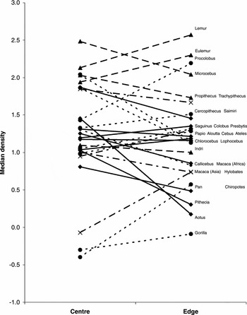
There were no significant differences in densities of primate species between the centre and the edges of their geographic ranges. This result held regardless of whether the analysis was by species or genera, or whether we used the area or distance definitions of centre and edge (N = 17–27; T > 15.5; P > 0.3 for all analyses; Figure 1 shows an example of the results for genera using the area analysis).
Comparison of log10-tranformed densities of genera at the centre and edge of their range, using the area-based definition of centre and edge. Each line represents a different genus. Dashed lines with triangle endpoints, Malagasy genera; dotted line with circular endpoints, African genera; solid lines with diamond endpoints, South American genera; dash dot line with × endpoints, Asian genera.

The mixed-effects linear model for the generic analysis by area confirmed the result of the Wilcoxon test, namely that there was no difference between densities at the centre versus the edge. The P-value for the centre/edge variable was consistently greater than 0.1 in all model versions. Similarly, census data from the studies by Peres (Reference PERES1993, Reference PERES1997) showed no overall difference in densities between centre and edge sites, although the sample was too small to analyse statistically (Appendix 3).
We also tested whether species or genera that decreased in density from centre to edge were different from those that did not in either number of dietary items or habitat types recorded. We did this by comparing the taxa that decreased in density to the extreme opposites, namely those that increased in density. We found no significant differences (N = 10 species per category, 5 genera per category, P > 0.3, Mann–Whitney U-test).
Effects of disturbance on density by genus
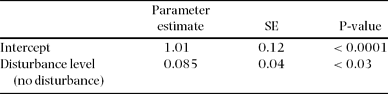
Although we found no geographic gradient in densities, there was a significant effect of disturbance on the densities of primate species. A mixed-effects linear model that included a random effect for genus, and fixed effects for disturbance and the residuals showed a significant effect of disturbance: densities were lower in the more disturbed sites (Table 1; r2 = 0.43, N = 216, P < 0.03). To assess model goodness of fit, we examined a scatterplot of residuals versus predicted values, and found no extreme residuals and no pattern of residuals with respect to the predicted values.
Output of the mixed-effects linear model. Model variables included a random effect for genus, a fixed effect for level of disturbance, and the residuals. Data were densities from the genera, by area analysis; N = 216 total data points in 21 genera.

To determine whether the effect of disturbance was masking a centre–edge gradient we assessed whether disturbed sites were unevenly distributed between the centre and edge of the generic ranges. They were not (N = 49 disturbed, 49 undisturbed in centre; 64 disturbed, 71 undisturbed in edge).
DISCUSSION
There was no evidence of a significant difference between densities in the centre versus the edge of geographic ranges of primates. This finding for a tropical taxon matches the result of many temperate studies, and adds to the conclusion that the gradient is not a general rule of biogeography. However, the sample of taxa was small, even if we found over 100 studies that provided data on densities.
In addition to testing the centre–edge gradient, we added a test of the influence of habitat heterogeneity, in our case in the form of anthropogenic disturbance. Disturbance correlated with a drop in density, irrespective of site in the geographic range, as was found in a study of neotropical sunbirds (Filloy & Bellocq Reference FILLOY and BELLOCQ2006).
Anthropogenic disturbance is merely one of a wide range of adverse conditions that can influence densities, none of which necessarily varies in intensity from centre to edge of geographic ranges (Sagarin Reference SAGARIN2006, Sagarin & Somero Reference SAGARIN and SOMERO2006). When the conditions do vary across the range, their effect can sometimes produce an increase in density toward the edge of a range, as when a decline in the intensity of interspecific competition toward the edge of the range allows an increase in density there (Stevens et al. Reference STEVENS, WILLIG and GAMARRA DE FOX2004).
However, given the likelihood of heterogeneity of the environment across the geographic range of most species, it might be useful for future searches for the equivalent of centre–edge gradients to be conducted over only occupied areas (i.e. a subset of the geographic range) rather than the entire geographic range, or over only the more environmentally homogeneous parts of the range. Even then, a heterogeneous distribution might exist (Vandermeer et al. Reference VANDERMEER, PREFECTO and PHILPOTT2008), in which case there could be a danger of wasted time spent on searching for non-existent environmental correlates or, worse, finding spurious correlates.
While the order Primates is well studied for a primarily tropical mammal, data are still woefully inadequate. The order contains hundreds of species and scores of genera (Groves Reference GROVES, Wilson and Reeder1993, Reference GROVES2001), and yet our sample contained 30 species and 27 genera with data on density in both centre and edge of ranges. Density is a measure of population size, which can affect probability of extinction. Knowledge of where in its range a species is likely to go extinct is surely vital for conservation. If so, primatology specifically and tropical biology in general need far more data (Coppeto & Harcourt Reference COPPETO and HARCOURT2005).
ACKNOWLEDGEMENTS
We would like to thank Mark Grote for statistical advice, especially in the development of the mixed-effects linear model. We would also like to thank Douglas A. Kelt, Andrew J. Marshall and the referees for detailed commentary that greatly improved the quality of the manuscript.
APPENDICES
Appendices are available as supplementary material on-line at http://journals.cambridgse.org/tro