2.1 Experimental set-up

The study focuses on isothermal subsonic jets issued from a round nozzle of exit diameter $D=50$  mm. The experiments were performed at the Bruit & Vent jet-noise facility of the Institut PPRIME, Poitiers, France. Boundary-layer transition inside the nozzle is forced using an azimuthally homogeneous carborundum strip of width $0.28D$ , whose downstream edge is located approximately $2.5D$ from the nozzle exit. The operating conditions are defined in terms of the nozzle-pressure ratio $NPR=P_{t}/P_{\infty }=1.7$ and nozzle temperature ratio $NTR=T_{t}/T_{\infty }=1.15$ . Here, the subscripts $t$ and $\infty$ refer to the stagnation (total) and free-stream (ambient) conditions respectively. The jet is isothermal ( $T_{j}/T_{\infty }=1.0$ ), and the jet Mach number is $M_{j}=U_{j}/c_{j}=0.9$ , where $U$ is the mean (time-averaged) jet exit streamwise velocity, $c$ is the speed of sound and the subscript $j$ refers to jet properties. With these conditions, the Reynolds number is $Re=\unicode[STIX]{x1D70C}_{j}U_{j}D/\unicode[STIX]{x1D707}_{j}\approx 1\times 10^{6}$ , where $\unicode[STIX]{x1D70C}$ is the density and $\unicode[STIX]{x1D707}$ is the dynamic velocity.

Details about the nozzle geometry, experimental configuration and noise postprocessing procedure are reported in appendices A and B. Some of these details are also available in the supplementary material (https://doi.org/10.1017/jfm.2018.476), along with measurements and LES data.

2.2 Numerical set-up

The present simulations use the LES framework developed at Cascade Technologies and leverage recent research efforts focused on modelling of the nozzle-interior turbulence (Brès et al. Reference Brès, Ham, Nichols and Lele2013, Reference Brès, Bose, Ham and Lele2014). The framework is composed of the preprocessing mesh-adaptation tool ‘Adapt’, the compressible flow solver ‘Charles’ and postprocessing tools for far-field noise prediction based on an efficient massively parallel implementation of the frequency-domain permeable formulation (Lockard Reference Lockard2000) of the Ffowcs Williams & Hawkings (Reference Ffowcs Williams and Hawkings1969) (FW–H) equation. Charles solves the spatially filtered compressible Navier–Stokes equations on general unstructured grids using a density-based finite-volume method. Time integration is explicit and uses the third-order total-variation diminishing Runge–Kutta (TVD RK) scheme of Gottlieb & Shu (Reference Gottlieb and Shu1998). The compressible fluxes are computed using a blend of central and upwind flux, resulting in a nominally second-order scheme in space. The computational set-up is briefly summarized below, with additional details about the solvers, the numerical schemes and the basic methodology available in Brès et al. (Reference Brès, Ham, Nichols and Lele2017). It should be noted that this reference does not cover the issues related to nozzle-interior turbulence modelling, which are the focus of the present work and are discussed in detail in what follows.

Figure 1.

Schematics of the flow configuration and simulation set-up: (a) overview of the computational domain; (b) spatial extent of the LES database; (c) modelling inside the nozzle.

Schematics of the numerical set-up are presented in figure 1, along with visualization of the instantaneous temperature and pressure field. The round nozzle geometry (with exit centred at $(x,r)=(0,0)$ ) is explicitly included in the axisymmetric computational domain, which extends from approximately $-10D$ to $50D$ in the streamwise ( $x$ ) direction and flares in the radial direction from $20D$ to $40D$ . A very slow coflow at Mach number $M_{\infty }=0.009$ is imposed outside the nozzle in the simulation ( $M_{\infty }=0$ in the experiment) to prevent spurious recirculation and facilitate flow entrainment. All other simulation settings match the experimental operating conditions, including the Reynolds number. The Vreman (Reference Vreman2004) subgrid model is used to account for the physical effects of unresolved turbulence on the resolved flow, with constant coefficient set to the recommended value of $c=0.07$ . A constant turbulent Prandtl number of $Pr_{t}=0.9$ is used to close the energy equation. To avoid spurious reflections at the downstream boundary of the computational domain, a damping function (Freund Reference Freund1997; Mani Reference Mani2012) is applied in the outflow buffer zone as a source term in the governing equations. In addition, the numerical operators are switched to lower-order dissipative discretization in the sponge zone for $x/D>31$ and $r/D>7$ to further damp turbulent structures and sound waves. Unless specified otherwise, all solid surfaces are treated as no-slip adiabatic walls.

In the preliminary parametric study, the far-field noise at $50D$ from the nozzle exit was calculated for three different FW–H surfaces consisting of a cylindrical surface of radius $0.65D$ up to $x/D=0$ followed by a conical surface extending to $x/D=30$ with different spreading rates of 0.11, 0.14 and 0.17. Here, the slopes are chosen based on estimates of the jet spreading rate (Zaman Reference Zaman1998, Reference Zaman1999). Similarly to previous studies (Brès et al. Reference Brès, Ham, Nichols and Lele2017), the results showed nearly identical spectra over the main frequency range for the three surfaces. The robustness of the prediction being thus confirmed, only the results from the intermediate surface outlined in black in figure 1(a) are reported. For treatment of the FW–H outflow disk, the method of ‘end-caps’ of Shur et al. (Reference Shur, Spalart and Strelets2005a ) is applied for $x\geqslant 25D$ , where the complex far-field pressures predicted from 11 FW–H surfaces with the same shape but outflow disks at different streamwise locations are phase-averaged. For all cases, the sampling period of the data recording on the FW–H surface is $\unicode[STIX]{x0394}t_{FWH}c_{\infty }/D=0.05$ .

Table 1 lists the settings and parameters for each LES run considered, including the time step $\text{d}t$ , the total simulation time $t_{sim}$ (after the initial transient is removed) and the data sampling period $\unicode[STIX]{x0394}t$ for the cases where the LES database of the full 3D flow field in primitive variables $(\unicode[STIX]{x1D70C},P,u,v,w)$ was collected, all expressed in acoustic time units (i.e. non-dimensionalized by $c_{\infty }/D$ ). The total computational cost is also reported in thousands of core hours. All of the calculations were carried out on the Cray XE6 system ‘Garnet’ (Opteron 16C 2.5 GHz processors, Cray Gemini interconnect, theoretical peak of 1.5 TFlop  $\text{s}^{-1}$ ) on 1024 and 5152 cores for the standard and refined grids respectively. The simulations with nozzle-interior turbulence modelling focused on adaptive isotropic mesh refinement of the internal boundary layer (prefix BL), synthetic turbulence (suffix Turb) and wall modelling inside the nozzle (suffix WM).

Table 1.

Simulation parameters: synthetic-turbulence amplitude $A=u_{trip}^{\prime }/u_{\unicode[STIX]{x1D70F}}$ , time step $\text{d}t$ , total simulation time $t_{sim}$ and database sampling period $\unicode[STIX]{x0394}t$ .

2.3 Mesh adaptation and near-wall refinement

The current meshing strategy has been used in previous jet studies (Brès et al. Reference Brès, Ham, Nichols and Lele2013, Reference Brès, Bose, Ham and Lele2014, Reference Brès, Jaunet, Le Rallic, Jordan, Colonius and Lele2015, Reference Brès, Jaunet, Le Rallic, Jordan, Towne, Schmidt, Colonius, Cavalieri and Lele2016) and promotes grid isotropy in the acoustic source-containing region through the use of adaptive refinement. The starting point is a coarse structured cylindrical grid with a paved core and clustering of points in the radial direction at the nozzle walls and lip. The grid contains approximately 0.4 million purely hexahedral control volumes. Several embedded zones of refinement with specific target length scale $\unicode[STIX]{x1D6E5}$ are then defined by the user and enforced iteratively by the adaptation tool, such that any cell with edge length (in any direction) greater than $\unicode[STIX]{x1D6E5}$ will be refined in that direction until the target length scale criterion is satisfied. The main refinement zone corresponds to the bulk of the mesh containing the jet plume, from $(x/D,r/D)=(0,1.5)$ to $(30,5)$ , with $\unicode[STIX]{x1D6E5}/D=0.14$ . Then, within that zone, three additional conical refinement regions focusing on the jet potential core and surrounding the FW–H surface are defined, from the nozzle lip to $(x/D,r/D)=(10,2.5)$ , $(7.5,2)$ and $(5.5,1.5)$ , with $\unicode[STIX]{x1D6E5}/D=0.1$ , $0.07$ and $0.04$ respectively. Finally, near the nozzle exit, three more refinement windows are centred on the lipline, extending to $x/D=2$ , $0.7$ and $0.5$ , with $\unicode[STIX]{x1D6E5}/D=0.02$ , $0.01$ and $0.0058$ respectively.

For the baseline cases, two grids were generated: a standard mesh containing approximately 10 million unstructured control volumes (cvs) and a refined mesh with 64 million cvs, by reducing the target length scale to a half in each refinement zone in the jet plume. It should be noted that for these cases, there is no specific near-wall or nozzle-interior refinement, and both grids have exactly the same coarse resolution inside the nozzle.

Table 2.

Representative mesh spacing at $r/D=0.5$ and corresponding number of grid points in the azimuthal direction $n_{\unicode[STIX]{x1D703}}$ .

In contrast, for the simulations involving nozzle-interior turbulence modelling, it can be anticipated that further mesh refinement is needed inside the nozzle to resolve the large-scale three-dimensional turbulent structures associated with the internal boundary layers. Therefore, isotropic refinement is added to the previous adaptation strategy and applied from the start of the boundary-layer trip at $x/D=-2.8$ to the nozzle exit at $x/D=0$ for a constant distance $0.085D$ from the nozzle wall and with target length scale $\unicode[STIX]{x1D6E5}/D=0.0075$ . The distance was chosen based on an initial estimate of the experimental nozzle-exit boundary-layer thickness, $\unicode[STIX]{x1D6FF}^{99}/D\approx 0.08$ , and the length scale was chosen to yield approximately 10–20 LES cells in the boundary layer. These choices lead to a finest wall-normal resolution of approximately 0.004D, after adaption. As part of a preliminary study focusing solely on the flow inside the nozzle, additional simulations were performed on two grids where the target length scale for the near-wall refinement was reduced to 0.0058 and 0.0029. These simulations yielded only limited improvements in the internal boundary-layer predictions for a significant increase in computational cost. Therefore, we chose the more practical approach of keeping the resolution inside the nozzle on the modest side for wall-bounded flows. Mesh details at the nozzle wall and lip are reported in table 2. The adapted grids with boundary-layer refinement now contain approximately 16 million and 69 million cvs for the standard and jet-plume refined cases respectively.

Figure 2.

Dimensionless mesh spacing (a) inside the nozzle at $x/D=-1$ , (b) at the nozzle exit $x/D=0$ and (c) at $x/D=2$ , in the axial ( $\unicode[STIX]{x0394}x/D$  — ⋅ —), radial ( $\unicode[STIX]{x0394}r/D$  – – –) and azimuthal ( $r\unicode[STIX]{x0394}\unicode[STIX]{x1D703}/D$  ——) directions, and equivalent cell length ( $vol^{1/3}/D$  — ○ —) for the grid 10M (top) and BL69M (bottom). The grids with the same mesh spacing are also reported in the figures (see table 1).

Figure 3.

Dimensionless mesh spacing along the lipline at $r/D=0.5$ in the axial ( $\unicode[STIX]{x0394}x/D$  — ⋅ —), radial ( $\unicode[STIX]{x0394}r/D$  – – –) and azimuthal ( $r\unicode[STIX]{x0394}\unicode[STIX]{x1D703}/D$  ——) directions, and equivalent cell length ( $vol^{1/3}/D$  — ○ —) for the grid (a) 10M and (b) BL69M. The grids with the same mesh spacing are also reported in the figures (see table 1).

Figure 4.

Dimensionless mesh spacing along the conical FW–H outline in the axial ( $\unicode[STIX]{x0394}x/D$  — ⋅ —), radial ( $\unicode[STIX]{x0394}r/D$  – – –) and azimuthal ( $r\unicode[STIX]{x0394}\unicode[STIX]{x1D703}/D$  ——) directions, and equivalent cell length ( $vol^{1/3}/D$  — ○ —) for the grid (a) 10M and (b) BL69M. The grids with the same mesh spacing are also reported in the figures (see table 1).

Figures 2–4 show, in logarithmic scale, the dimensionless mesh spacings for the four grids at different streamwise locations, along the lipline and along the outline of the conical section of the FW–H surface respectively. In contrast to fully structured grids, the mesh length scales for the present unstructured grids with adaptation and hanging nodes are not globally predefined with smooth analytical form and vary in space depending on the refinement target length scales. The locations of the user-defined grid transitions are clearly visible in the figures, in particular for the azimuthal length scale (red solid curve) in figure 3 at $x/D=0.5$ , 2, 5.5, etc. Nevertheless, the present isotropic refinement strategy leads to similar mesh spacings in all three axial, radial and azimuthal directions for most of the relevant regions of the computational domain. In terms of mesh isotropy, the only noticeable exception is near the lipline, where the small radial resolution, present in the initial structured cylindrical grid to resolve the nozzle lip, remains in the adapted grids and leads to more anisotropy in the downstream region of the jet plume (see figure 3). The effect is, however, localized and, overall, the cell aspect ratio (i.e. largest over smaller mesh length scale) is less than 2 for 85 % (97 %) of the cvs within the FW–H surface for the grid without (with) jet-plume refinement. The equivalent cell length, $vol^{1/3}/D$ , which is the cubic root of the cell volume, is therefore a representative metric of the resolution for the present isotropic hexahedral-dominant grids and is also presented in the figures. Following the analysis of Mendez et al. (Reference Mendez, Shoeybi, Sharma, Ham, Lele and Moin2012) and Brès et al. (Reference Brès, Ham, Nichols and Lele2017), this quantity is also used to estimate the limit Strouhal number $St_{lim}$ of acceptable resolution, corresponding to a wave resolved with eight grid points per wavelength: $St_{lim}=D/(8vol^{1/3}M_{a})$ , where $M_{a}=U_{j}/c_{\infty }$ is the acoustic Mach number. Because the high-frequency noise sources are typically expected in the jet plume between the nozzle exit and the end of the potential (i.e., $0<x\lesssim 10$ ), the present grids are designed to approximately resolve the radiated noise spectra up to $St_{lim}\approx 2$ for the standard mesh and to $St_{lim}\approx 4$ for the refined mesh, based on the resolution on the FW–H surface in that region.

2.4 Synthetic turbulence

An extension to the digital filtering technique of Klein, Sadiki & Janicka (Reference Klein, Sadiki and Janicka2003) was implemented for the generation of synthetic turbulence on unstructured grids for both inflow boundary and wall boundary conditions. Because the turbulence levels inside the exhaust system upstream of the nozzle are typically unknown, the main objective of the synthetic turbulence is to seed the flow with fluctuations of reasonable amplitude, length and time scales, such that realistic turbulence is fully developed by the nozzle exit.

In the present work, synthetic-turbulence boundary conditions are used to model the boundary-layer trip present in the experiment at $-2.8<x/D<-2.5$ on the internal nozzle surface (see figure 1 c). Based on the initial estimate of the experimental nozzle-exit boundary-layer thickness, the trip is therefore located more than $30\unicode[STIX]{x1D6FF}^{99}/D$ from the nozzle exit, which is sufficient for the spatial development of a turbulent boundary layer.

The wall friction velocity $u_{\unicode[STIX]{x1D70F}}$ is often used as a scaling parameter for the fluctuating component of velocity in wall-bounded turbulent flows. An initial value for $u_{\unicode[STIX]{x1D70F}}$ was estimated based on the average wall shear stress downstream of the trip location for preliminary simulation on the 16M mesh. Fluctuations were then introduced in each component of the zero-mean velocity field at the wall boundary faces of the trip, with a prescribed amplitude $u_{trip}^{\prime }=Au_{\unicode[STIX]{x1D70F}}/\sqrt{3}$ . As part of the initial parametric studies, two different amplitudes, $A=0.8$ and 2, were used, with the former value applied for most of the computations. For all cases, $\unicode[STIX]{x1D6E5}_{max}$ and $2\unicode[STIX]{x1D6E5}_{max}/u_{trip}^{\prime }$ were used as initial estimates of the length and time scales of the input fluctuations, where $\unicode[STIX]{x1D6E5}_{max}=\max (\unicode[STIX]{x0394}x,\unicode[STIX]{x0394}r,r\unicode[STIX]{x0394}\unicode[STIX]{x1D703})$ is the largest mesh spacing at the location of the trip (see table 2). Physically, this can be interpreted as the introduction of isotropic eddies of turbulent kinetic energy $1/2(Au_{\unicode[STIX]{x1D70F}})^{2}$ and dimensions comparable to the local mesh size. Here, the chosen length scale is also similar to the thickness of the experimental trip.

While the present work focuses on the $M_{j}=0.9$ case, different Mach number conditions ranging from 0.4 to 0.9 were considered as part of a broader LES study, and nearly identical initial estimates, $u_{\unicode[STIX]{x1D70F}}/U_{j}\approx 0.042$ , were obtained in all cases. Similar values can be obtained using simple flat-plate zero-pressure-gradient turbulent boundary-layer approximations. Assuming the classical form of the skin-friction coefficient in turbulent flows, $c_{f}=0.0576Re_{x}^{-1/5}$ , with $x$ as the distance between the start of the straight section of the nozzle and the boundary-layer trip, the empirical value of the wall friction velocity at the trip would be between $u_{\unicode[STIX]{x1D70F}}/U_{j}\approx 0.041$ and 0.044 for $M_{j}=0.9$ –0.4. These estimates further confirmed the choice of order of magnitude for the coefficient $A=O(1)$ .

2.5 Wall modelling

When active, the equilibrium wall model, based on the work of Bodart & Larsson (Reference Bodart and Larsson2011) and Kawai & Larsson (Reference Kawai and Larsson2012), is applied inside the nozzle in the straight-pipe section between the boundary-layer trip and the nozzle exit (see figure 1 c). The present method falls in the category of the wall-stress modelling approach (see reviews by Piomelli & Balaras Reference Piomelli and Balaras2002; Larsson et al. Reference Larsson, Kawai, Bodart and Bermejo-Moreno2016): unlike hybrid RANS/LES and detached-eddy simulations (Spalart Reference Spalart2009) that solve the unsteady Navier–Stokes equations on a single grid, with a RANS model near the wall and a LES model in the rest of the domain, the unstructured LES grid is formally defined as extending all the way to the wall (i.e. identical to a simulation without wall model), and a separate (structured) grid is embedded near the wall to solve the 1D RANS equations. The RANS solver takes information from the computed LES flow field a few cells away from the wall, and returns back the shear stress $\unicode[STIX]{x1D70F}_{w}$ and the heat transfer $q_{w}$ at the wall, to be used as boundary conditions for the LES wall-flux computation.

For most convex surfaces, the RANS grid is a simple extrusion of the wall surface mesh along the normal vector of each wall face. Following the recommendations of Kawai & Larsson (Reference Kawai and Larsson2012), the wall-model-layer thickness (i.e. the distance from the wall where the RANS solver takes the LES information) is set to at least three LES cells away from the wall. In previous work (Brès et al. Reference Brès, Ham, Nichols and Lele2013), various sizes and stretching coefficients were considered for the inner-layer RANS grid, and the default values of 40 cells and 10 % stretching are used in the present study for a wall-normal grid spacing in wall units of $y_{RANS}^{+}=O(1)$ . As shown in table 1, for the present cases with no specific attempt to optimize the performance, the extra computational cost of the wall model is approximately 27 % of the stand-alone LES cost, similar to the value of 30 % reported by Bodart & Larsson (Reference Bodart and Larsson2011). Load balancing of the wall-model procedure has been suggested as an approach to potentially reduce this additional cost.

3.1 Effects of nozzle-interior turbulence modelling on flow-field results

3.1.2 Nozzle-exit velocity statistics

Nozzle-exit profiles of velocity statistics are plotted in figure 6. Both experimental hot-wire measurements and LES results are reported at the same location just downstream of the nozzle exit, at $x/D=0.04$ . The slight mismatch in mean velocity for $r/D>0.5$ is caused by the small coflow $M_{\infty }=0.009$ imposed in the simulation.

Figure 6.

Nozzle-exit boundary-layer profiles at $x/D=0.04$ of (a) the mean streamwise velocity and (b–d) the RMS values of the fluctuating velocity components: experiment (▫ hot wire), baseline LES 10M (– – –) and 64M (——, green), and LES with nozzle-interior turbulence modelling BL16M (— ⋅ —), BL16M_Turb2 (

, magenta), BL16M_Turb (——, cyan), BL16M_WM (— ⋅ —, blue), BL16M_WM_Turb2 (

, orange) and BL16M_WM_Turb (——, red).

For both baseline cases, the mean (time-averaged) streamwise velocity profiles are identical and correspond to the typical laminar profile. The turbulence intensities in figure 6(b–d) all show similar characteristics, with a single wider peak and lower root mean square (RMS) values. In contrast, the nozzle-exit boundary layer in the experiment is turbulent, thanks to the azimuthally homogeneous carborundum strip upstream in the pipe. The RMS peaks are therefore largely underpredicted and the boundary layer is too thin for both LES 10M and 64M.

With isotropic near-wall grid refinement, all of the nozzle-exit boundary layers now exhibit turbulent mean and RMS velocity profiles, with larger fluctuation levels near the wall. Much like the nozzle-exit boundary-layer measurements of Fontaine et al. (Reference Fontaine, Elliot, Austin and Freund2015), the present turbulence intensity profiles feature two distinct regions. The first region, which Fontaine et al. (Reference Fontaine, Elliot, Austin and Freund2015) refer to as the ‘boundary-layer remnant’, is characterized by a relatively shallow rise, up to $r/D\approx 0.47$ in our study. This region is here present in both experiment and simulations, and, for the simulation, is sensitive to the amplitudes of synthetic turbulence and/or presence of wall modelling. The second region, which they associate with the inflectional instability of the free shear profile, is characterized by a sharp peak in RMS levels near $r/D\approx 0.5$ . In that region, the LES results collapse onto two distinct curves, depending on whether or not wall modelling is used. While the nozzle-exit RMS levels are overpredicted compared with experiment for cases BL16M, BL16M_Turb and BL16M_Turb2 (see figure 6 b), the cases with wall modelling show less overshoot and better agreement. Here, the effect of the wall model is significant and beneficial: the most important region in terms of the initial growth rate of wavepackets is this ‘shear-layer’ region, where the correct RMS underpins the correct velocity gradient. Overprediction of near-wall fluctuations is a characteristic feature of under-resolved LES. Even the present choice of 20 points across the nozzle-exit boundary-layer thickness is coarse in terms of viscous units at the wall. Based on the resolution in the first LES cell from the nozzle internal surface, the wall-normal grid spacing in wall units $y_{LES}^{+}$ is in the 130–175 range, and approximately 200–240 for the streamwise and azimuthal grid spacing, depending on the case and streamwise location. In a corresponding DNS, the typical values would be approximately 1 in the normal direction, 10–20 in the streamwise direction and 5–10 in the azimuthal direction. Therefore, the turbulent boundary layer needs to be in the wall-modelled LES regime. The physics in the viscous sublayer is now modelled with the 1D RANS, leading to an average $y_{RANS}^{+}\approx 0.7$ for the first RANS cell.

Finally, the addition of synthetic turbulence has less impact than mesh refinement and wall modelling. Two different levels of amplitudes for the synthetic turbulence were tested (see table 1), and the change in fluctuation amplitude can clearly be seen in figure 5 at the location of the trip, for instance in the cases BL16M_Turb and BL16M_Turb2. However, as more realistic turbulence develops, the differences in flow structures at the wall only persist for approximately $0.5D$ downstream of the trip, and visually similar turbulent boundary layers are then observed beyond that point. As shown in figure 6, the nozzle-exit boundary-layer profiles in the ‘shear-layer’ region are essentially independent of the initial choice (or absence) of synthetic fluctuations. The main discernible differences are observed in the ‘boundary-layer remnant’, where the turbulence levels in the nozzle core flow away from the walls are slightly larger with the high-amplitude synthetic turbulence.

Figure 7.

Profiles along the centreline and lipline of (a,b) mean and (c,d) RMS streamwise velocity: experiment (▫ hot wire, ○ PIV), baseline LES 10M (– – –) and 64M (——, green), and LES with nozzle-interior turbulence modelling BL16M (— ⋅ —), BL16M_Turb2 (

, magenta), BL16M_Turb (——, cyan), BL16M_WM (— ⋅ —, blue), BL16M_WM_Turb2 (

, orange) and BL16M_WM_Turb (——, red).

3.1.3 Centreline and lipline profiles

The streamwise velocity statistics along the centreline and lipline (i.e. $r/D=0.5$ ) in figure 7 also show improved results for the LES cases with nozzle-interior turbulence modelling. The most drastic change can be observed in the fluctuation amplitude along the lipline in figure 7(d), where the fluctuation overshoot around $x=0.5D$ (related to the shear-layer laminar-to-turbulent transition) is present in both baseline LES, independent of the resolution in the jet plume, but is nearly removed with improved treatment of the internal nozzle dynamics.

For the centreline profiles, the main feature is the underprediction of the length of the potential core $x_{c}$ (defined as the distance up to which the streamwise velocity is greater than 95 % of the jet exit velocity) for the baseline case 10M. The early termination of the potential core results in a shift of the peak RMS levels further upstream. As expected, the grid refinement in the jet plume for the case 64M slightly improves the prediction of turbulent mixing, and of $x_{c}$ , but the RMS level remains well underpredicted. Better improvements are actually obtained on the standard mesh for all of the cases with nozzle-interior turbulence modelling. Inside the nozzle, all of the simulations show very low nozzle core-turbulence levels (see the inset in figure 7 c). As discussed in the previous section, slightly larger values are observed for the two cases with high initial amplitude of the synthetic turbulence (i.e. suffix Turb2).

Overall, the wall-modelled LES cases provide arguably the best match with the particle-image velocimetry (PIV) measurements, in particular in the very-near-nozzle region $x/D<0.5$ . Due to the relatively short simulation time used for these preliminary comparisons, the statistics show some variations between the different cases, in particular for $x/D>8$ , in the fully developed mixing jet region downstream of the potential core, where the statistics are more significantly underpinned by low frequencies, difficult to converge with the short simulation time. Higher-order moments such as RMS and skewness are, of course, more sensitive to statistical convergence and spatial resolution. Specifically, some of the sharp changes in slope in the RMS profiles are related to transitions in mesh resolution, as corroborated by the mesh spacing curves in figure 3. These features are discussed in greater detail in § 4.1 for the LES with extended simulation time and additional refinement in the jet plume.

Figure 8.

Spectra of pressure and velocity fluctuations along the lipline at (a) $(x/D,r/D)=(-0.05,0.48)$ , (b) $(0.5,0.5)$ and (c) $(5,0.5)$ : baseline LES 10M (– – –) and 64M (——, green), and LES with nozzle-interior turbulence modelling BL16M (— ⋅ —), BL16M_Turb2 (

, magenta), BL16M_Turb (——, cyan), BL16M_WM (— ⋅ —, blue), BL16M_WM_Turb2 (

, orange) and BL16M_WM_Turb (——, red). The arrows indicate the frequencies of the trapped acoustic waves (see appendix D).

3.1.4 Pressure and velocity fluctuation spectra

Figure 8 shows the power spectral density (PSD) of the pressure fluctuations (in $\text{dB}/St$ ) and of the three components of the velocity fluctuations in cylindrical coordinates (non-dimensionalized by $U_{j}^{2}/St$ ) as a function of frequency in Strouhal number $St=fD/U_{j}$ . The spectra are directly computed from the flow-field time histories recorded along the lipline at $(x/D,r/D)=(-0.05,0.48)$ , $(0.5,0.5)$ and $(5,0.5)$ for 36 equally spaced locations in the azimuthal direction. Because of the azimuthal symmetry of the geometry, these locations are statistically equivalent and the resulting spectra are azimuthally averaged.

The first position, $(x/D,r/D)=(-0.05,0.48)$ , is representative of the near-wall flow inside the nozzle. As expected, for the baseline cases 10M and 64M with initially laminar boundary layers, the velocity fluctuations have much lower levels and no discernible high-frequency content. In contrast, all of the simulations with nozzle-interior flow modelling display turbulent spectra with broadband frequency content. For these cases, the velocity spectra collapse onto two curves of similar shape but different amplitude, depending on whether wall modelling is applied or not. As mentioned in the previous section, overprediction of near-wall fluctuations is a characteristic feature of under-resolved LES, and all of the simulations without wall modelling exhibit higher levels of velocity fluctuation. At this location, the velocity spectra are independent of the initial choice (or absence) of synthetic fluctuations, much like the nozzle-exit velocity profiles in the ‘shear-layer’ region discussed in § 3.1.2. In contrast, the pressure spectra show some sensitivity to the synthetic-turbulence parameters; namely, higher initial amplitude of the synthetic turbulence inside the nozzle leads to higher levels of pressure fluctuation in the mid- to high-frequency range. Here, another interesting feature is the presence of tones in the pressure spectra at specific frequencies for all of the simulations. Some of the tones are also visible in the velocity spectra of the baseline cases 10M and 64M because of the low fluctuation levels. These discrete tones are characteristics of a novel class of resonant acoustic waves which are trapped within the potential core of the jets and transmit some of the energy into the nozzle (see appendix D).

The second position, $(x/D,r/D)=(0.5,0.5)$ , corresponds to the location of peak RMS overshoot along the lipline related to the shear-layer laminar-to-turbulent transition in the baseline LES. Therefore, higher fluctuation levels are observed for both cases 10M and 64M with an initially laminar jet compared with all of the other cases with an initially turbulent jet, in particular in the pressure spectra. For the simulations with nozzle-interior flow modelling, all of the spectra now collapse on a single broadband curve, independently of the use of a wall model or the presence/initial amplitude of the synthetic turbulence inside the nozzle. Here, some of the tones associated with the trapped acoustic waves are still visible, while others have been overwhelmed by the increased turbulence levels.

The third position, $(x/D,r/D)=(5,0.5)$ , is located along the lipline towards the end of the potential. As the turbulence continues to develop, the fluctuation levels increase and the spectra shift to lower frequencies, with similar shape and frequency content for all of the simulations and variables. In the inertial subrange, all of the spectra follow the expected slope of energy cascade in isotropic turbulence, i.e. $-7/3$ for pressure and $-5/3$ for velocity, up to the grid cutoff frequency $St\approx 3.5$ . The only noticeable exception is the case 64M with refinement in the jet plume, in which the added grid resolution leads to a higher cutoff frequency of around $St\approx 6.8$ .

Figure 9.

(a–c) Power spectral density of pressure on the polar microphone array at $50D$ from the nozzle exit at various angles $\unicode[STIX]{x1D719}$ , and (d) OASPL: experiment (○), baseline LES 10M (– – –) and 64M (——, green), and LES with nozzle-interior turbulence modelling BL16M (— ⋅ —), BL16M_Turb2 (

, magenta), BL16M_Turb (——, cyan), BL16M_WM (— ⋅ —, blue), BL16M_WM_Turb2 (

, orange) and BL16M_WM_Turb (——, red).

3.2 Effects of nozzle-interior turbulence modelling on far-field acoustic results

Figure 9 compares the PSD of pressure fluctuations and the overall sound pressure level (OASPL) between experiment and LES cases with and without nozzle-interior turbulence modelling. The PSD is computed with the Welch method (block size of 2048, 75 % overlap), bin-averaged (bin size $\unicode[STIX]{x0394}St=0.05$ ) and reported in $\text{dB}/St$ , following the same non-dimensionalization as the experiment (see appendix B). Similarly to the direct computation of spectra discussed in § 3.1.4, the FW–H predictions are performed for 36 equally spaced microphones distributed along the azimuthal angle, and the resulting spectra are azimuthally averaged. The same procedure is applied for calculation of the OASPL in dB, where the frequency range considered for the integration is $0.05\leqslant St\leqslant 3$ . To evaluate uncertainty in the experimental noise data, basic techniques were used to estimate the errors due to the microphone sensitivity, statistical errors and errors associated with measurement repeatability. The latter was found to be the main source of uncertainty, in general less than 0.5 dB.

For the baseline cases 10M and 64M, the noise spectra are reasonably well captured up to $St\approx 1$ . For higher frequencies, however, the noise levels from these simulations are overpredicted by the same amount for both grids, indicating that refinement in the jet plume will not reduce the discrepancy. This is observed for sideline angles in the range $90^{\circ }\leqslant \unicode[STIX]{x1D719}\leqslant 120^{\circ }$ , where the large-scale mixing noise is less dominant. For shallow angles to the jet axis, e.g. $\unicode[STIX]{x1D719}=150^{\circ }$ , this high-frequency overprediction is less severe, but the peak radiation around $St=0.2$ is now underpredicted. These trends translate into discrepancies of approximately 1.5–2 dB in the OASPL, with overprediction at sideline angles and underprediction aft.

With nozzle-interior turbulence modelling, the overprediction observed at high frequencies is eliminated, with the notable exception of the case with high-amplitude synthetic turbulence (i.e. suffix Turb2). For these cases, there is an evident change of slope and excess high-frequency noise for $St>2$ particularly visible at sideline angles, which is probably related to the increase in pressure fluctuations and core-turbulence levels inside the nozzle, as previously discussed. The same trends have been reported in the experimental study by Zaman (Reference Zaman2012), where larger spectral amplitudes were observed with the application of turbulence-generating grids. In the experiment, the increase was also generally more pronounced at $90^{\circ }$ and higher frequencies.

Aside from these two cases, good agreement with experimental measurements is obtained for the present mesh, which is of modest size, at all angles and frequencies up to $St\approx 2{-}3$ , consistent with the estimate from the grid design. The resulting OASPL directivity curve in figure 9(d) now generally lies within experimental uncertainty, with less than 1 dB difference for most angles. The discrepancies appear to be mostly due to the variations in low frequencies related to the relatively short simulation time (see the statistical convergence and grid resolution study in § 4.1). Like the flow-field results discussed in the previous section, it was found that the grid adaptation has the most significant impact on far-field noise predictions, while the low-amplitude synthetic turbulence and wall model have more subtle effects. With the exception of the two LES cases with high input turbulence, the spectra do not contain discernible tones or visible numerical artefacts that could be directly related to the added modelling inside the nozzle.

4.1 Database validation: statistical convergence and grid resolution study

Based on the results presented above, the turbulent case BL16M_WM_Turb and laminar case 10M were selected for further analysis and comparisons. The total simulation time in both cases was increased to $t_{sim}c_{\infty }/D=2000$ . Finally, to investigate grid convergence, an additional simulation for the same configuration and numerical set-up as BL16M_WM_Turb was performed on the refined mesh, i.e. the 69 million cv grid with double the resolution in the jet plume (see table 1).

Figure 10.

Contours of (a) mean and (b) RMS streamwise velocity in the midsection plane ( $z=0$ ): experimental PIV (top row), extended baseline LES 10M and extended LES with nozzle-interior turbulence modelling BL16M_WM_Turb and BL69M_WM_Turb.

Figure 11.

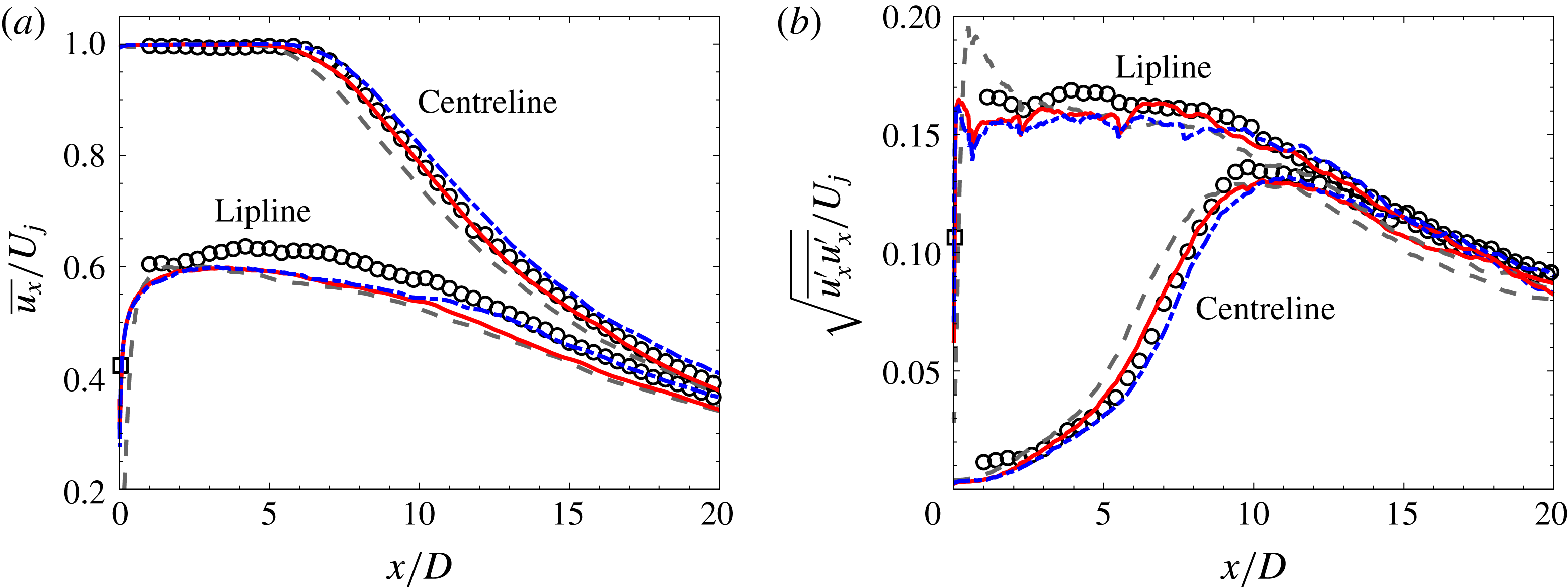
Centreline and lipline profiles of (a) mean and (b) RMS streamwise velocity: experiment (▫ hot wire, ○ PIV), extended baseline LES 10M (– – –) and extended LES with nozzle-interior turbulence modelling BL16M_WM_Turb (——) and BL69M_WM_Turb (— ⋅ —).

4.1.1 Jet-plume statistics

Figure 10 shows comparisons of the streamwise velocity statistics in the jet plume between PIV and LES for the extended simulations. The corresponding centreline and lipline profiles are presented in figure 11. It should be noted that reliable PIV measurements are not available for $x/D<1$ because of edge effects and lack of seeding homogeneity near the nozzle (see appendix A).

Despite the significant differences in grid resolution in the jet plume, both simulations BL16M_WM_Turb and BL69M_WM_Turb with nozzle-interior turbulence modelling give similar flow-field results, both in good agreement with the experimental measurements. Compared with the profiles in figure 7 with statistics computed over 600 acoustic time units (i.e. the duration from the preliminary study), the predictions for the extended simulations show improvements in the statistical convergence. The mesh refinement in the jet plume for case BL69M_WM_Turb also provides some improvements of the artefacts associated with transitions in mesh resolution. As mentioned in § 3.1, the discontinuities in RMS levels observed at $x/D\approx 0.5$ , 2.1 and 5 in figures 10(b) and 11(b) correspond to unstructured grid transitions. With smaller changes in grid spacing on the refined mesh, the grid imprint on RMS levels is reduced in the refined case. For both extended simulations with nozzle-interior turbulence modelling, the length of the potential core $x_{c}$ is well predicted (see table 3). As expected, grid refinement in the jet plume tends to increase the value of $x_{c}$ and shift the centreline peak RMS fluctuations further downstream. Likewise, after the end of the potential core, the refined case tends to display slightly higher mean and RMS values than the standard case, as the increase in resolution in that region leads to prediction improvements of the turbulent mixing.

Figure 12.

Profiles of the shear-layer momentum thickness $\unicode[STIX]{x1D6FF}_{\unicode[STIX]{x1D703}}$ : experiment (▫ hot wire, ○ PIV, —— linear interpolation), extended baseline LES 10M (– – –) and extended LES with nozzle-interior turbulence modelling BL16M_WM_Turb (——, red) and BL69M_WM_Turb (— ⋅ —).

4.1.2 Nozzle-exit conditions and shear-layer development

The shear-layer momentum thickness $\unicode[STIX]{x1D6FF}_{\unicode[STIX]{x1D703}}$ is presented in figure 12. Similarly to Bogey & Bailly (Reference Bogey and Bailly2010), $\unicode[STIX]{x1D6FF}_{\unicode[STIX]{x1D703}}$ is estimated as

(4.1) $$\begin{eqnarray}\displaystyle \unicode[STIX]{x1D6FF}_{\unicode[STIX]{x1D703}}(x)=\int _{0}^{r_{0.05}}\frac{\overline{u_{x}}(x,r)}{\overline{u_{x}}(x,0)}\left(1-\frac{\overline{u_{x}}(x,r)}{\overline{u_{x}}(x,0)}\right)\text{d}r, & & \displaystyle\end{eqnarray}$$

where $\overline{u_{x}}$ is the time- and azimuthal-averaged streamwise velocity. The integral radial bound $r_{0.05}$ accounts for the slow coflow and corresponds to the distance where $\overline{u_{x}}(x,r_{0.05})-U_{\infty }=0.05\overline{u_{x}}(x,0)$ . The same approach is used to estimate the displacement thickness $\unicode[STIX]{x1D6FF}^{\ast }$ . Table 3 summarizes all of the nozzle-exit boundary-layer properties predicted from simulations and estimated from the experimental PIV using linear extrapolation to $x/D=0$ . As the shape factor $H=\unicode[STIX]{x1D6FF}^{\ast }/\unicode[STIX]{x1D6FF}_{\unicode[STIX]{x1D703}}$ varies from 2.59 for fully laminar flow to approximately 1.4 for fully turbulent flow (Schlichting & Gertsen Reference Schlichting and Gertsen2000), the results confirm the initially laminar and turbulent state of the jets for the different LES. Here, the estimated momentum thickness is also comparable to the values $\unicode[STIX]{x1D6FF}_{\unicode[STIX]{x1D703}}/D\approx 0.0055$ –0.0213 reported in the recent experiments by Fontaine et al. (Reference Fontaine, Elliot, Austin and Freund2015) with similar convergent-straight nozzles and operating conditions.

Figure 13.

Profiles of the mean streamwise velocity (a) in the near-nozzle region and (b) in the jet plume: experiment (▫ hot wire, ○ PIV), extended baseline LES 10M (– – –) and extended LES with nozzle-interior turbulence modelling BL16M_WM_Turb (——) and BL69M_WM_Turb (— ⋅ —).

Table 3.

Estimates of the jet potential core length $x_{c}$ , nozzle-exit boundary-layer momentum thickness $\unicode[STIX]{x1D6FF}_{\unicode[STIX]{x1D703}}$ , displacement thickness $\unicode[STIX]{x1D6FF}^{\ast }$ , thickness $\unicode[STIX]{x1D6FF}^{99}$ and shape factor $H$ .

Figure 14.

Profiles of the RMS streamwise velocity (a) in the near-nozzle region and (b) in the jet plume: experiment (▫ hot wire, ○ PIV), extended baseline LES 10M (– – –) and extended LES with nozzle-interior turbulence modelling BL16M_WM_Turb (——) and BL69M_WM_Turb (— ⋅ —).

Figures 13 and 14 show the evolution of the mean streamwise velocity and streamwise turbulence intensity at different axial locations upstream and downstream of the nozzle exit. As previously discussed, both LES cases BL16M_WM_Turb and BL69M_WM_Turb have the same adapted mesh inside the nozzle and the same synthetic turbulence and wall modelling applied to the nozzle internal walls. This leads to identical profiles for $x/D<0$ and similar integral quantities for the nozzle-exit boundary layer. The only noticeable difference is at $x/D=0.04$ in figure 14(a) for the maximum RMS levels around $r/D=0.5$ , where the additional resolution in the jet plume for the refined case is better suited to resolving the strong velocity gradients and sharp peak of the RMS levels at the lipline. That peak is missed in the measurement because of limited spatial resolution. For both simulations, the linear growth of the shear layer starts almost immediately at the nozzle exit and closely matches the experimental value in figure 12.

In contrast, for the initially laminar jet in simulation 10M, the jet flow development is characterized by different features in three distinct regions. Inside the nozzle, the boundary layer is laminar and the jet remains laminar with limited spreading close to the nozzle exit, up to $x/D\approx 0.2$ (see the inset in figure 12). This is followed by a rapid growth related to the shear-layer laminar-to-turbulent transition, as indicated by the overshoot of the velocity RMS around $x/D=0.5$ in figure 11 and figure 14(a). This process then leads to enhanced mixing further downstream, resulting in the larger spreading rate observed in figure 12 and earlier termination of the potential core. Overall, the trends for the potential core length and shear-layer growth are consistent with the results reported by Bogey & Bailly (Reference Bogey and Bailly2010) for simulations of initially laminar jets at Mach 0.9.

4.1.3 Far-field acoustics

In addition to the single microphone in the far field, pressure measurements were also made using an 18-microphone azimuthal ring array whose axial position was varied in order to map the sound field on a cylindrical surface of radius $r/D=14.3$ centred on the jet axis. This microphone ring was also used to perform the azimuthal decomposition of the radiated noise discussed in § 4.2. The complete comparison with the LES predictions is presented in figure 15 for all microphones, with the corresponding OASPL directivity shown in figure 16.

Figure 15.

Power spectra density of pressure (a) on the cylindrical microphone array of radius $r=14.3D$ and (b) on the polar microphone array at $50D$ from the nozzle exit for the different angles $\unicode[STIX]{x1D719}$ : experiment (○), extended baseline LES 10M (– – –) and extended LES with nozzle-interior turbulence modelling BL16M_WM_Turb (——) and BL69M_WM_Turb (— ⋅ —).

First, for the initially laminar jet, the results of the extended simulation 10M confirm the conclusion of the preliminary study: the noise spectra are reasonably well predicted for most angles up to frequency $St\approx 1$ , with overprediction at higher frequencies and slight underprediction of the peak radiation around $St=0.2$ . The discrepancies are more pronounced on the cylindrical microphone array (see the zoomed-in view of the spectra in figure 18) and lead to the mismatch in shape for the noise directivity observed in the OASPLs in figure 16. Experimental studies by Brown & Bridges (Reference Brown and Bridges2006), Zaman (Reference Zaman2012) and Karon & Ahuja (Reference Karon and Ahuja2013) all reported similar increased levels at high frequencies for subsonic jets with (nominally) laminar initial shear layers compared with jets with (nominally) turbulent ones. In particular, Brown & Bridges (Reference Brown and Bridges2006) applied a thin wrap of reticulated foam metal (RFM) inside their nozzle to trip the boundary layer, similar to the carborundum strip used in the present experiments. The RFM inserts changed the characteristics of the nozzle-exit boundary layer from laminar to turbulent and eliminated the high-frequency noise.

For the initially turbulent jets, there is little variation between the results from the standard and refined simulations for most angles and relevant frequencies. With the extended simulation time, the low-frequency part of the spectrum shows better convergence compared with the preliminary results in figure 9 and the predictions are further improved, now typically within 0.5 dB of the measurements. The main discernible differences between the spectra from the two LES are observed in the grid cutoff frequency for high angles $\unicode[STIX]{x1D719}\geqslant 150^{\circ }$ : at these angles, the limit frequency is approximately $St\approx 2$ for the standard case BL16M_WM_Turb and $St\approx 4$ for the refined case BL69M_WM_Turb with double the resolution in the jet plume. Here, it is important to note that these discrepancies are outside the main frequency range of interest and have levels 25–30 dB lower than the peak radiated noise, such that they do not significantly impact the predictive capabilities or use of the database for sound-source modelling. Overall, the statistical convergence and grid resolution studies provide thorough validation and confidence in the LES database of the case BL16M_WM_Turb for flow and noise data up to $St\approx 2{-}3$ . All of the remaining analysis is therefore conducted using that longer database.

Figure 16.

Overall sound pressure level directivity (a) on the cylindrical microphone array of radius $r=14.3D$ and (b) on the polar microphone array at $50D$ from the nozzle exit: experiment (○), extended baseline LES 10M (– – –) and extended LES with nozzle-interior turbulence modelling BL16M_WM_Turb (——) and BL69M_WM_Turb (— ⋅ —).

4.1.4 Near-field acoustics

For the eduction of wavepacket signatures and further investigation of the tones observed in the LES spectra inside the nozzle, the experiment was also instrumented with a 48-microphone cage array consisting of six azimuthally equispaced microphones at seven different locations in the near field on the jet. Figure 17 shows the comparison with the LES predictions at three representative locations, namely (a) $(x/D,r/D)=(0.12,0.72)$ , (b) $(2.00,0.91)$ and (c) $(4.47,1.33)$ .

For the microphone ring closest to the nozzle exit, corresponding to a jet inlet angle of $\unicode[STIX]{x1D719}\approx 99.5^{\circ }$ , the discrete tones associated with the resonant acoustic waves are again observed in the spectra, consistent with the results inside the nozzle discussed in § 3.1.4. For both simulations with an initially turbulent jet, the shape of the spectra and the frequency and amplitude of the tones closely match the experimental measurements. For the simulation with an initially laminar jet, the tones are still present at the same frequencies but the overall levels are higher because of the enhanced noise radiation related to the shear-layer laminar-to-turbulent transition. Additional analysis of the discrete tones is presented in appendix D.

For the near-field microphones further downstream, the same conclusions hold in terms of agreement with experiment for the simulations with an initially turbulent jet and overprediction for the simulation with an initially laminar jet. At these locations corresponding to the peak radiation angles (i.e. $\unicode[STIX]{x1D719}\approx 153.9^{\circ }$ and $163.4^{\circ }$ ), the spectral levels are much higher and there is no visible tonal component. As discussed in detail in the work of Schmidt et al. (Reference Schmidt, Towne, Colonius, Cavalieri, Jordan and Brès2017) and Towne et al. (Reference Towne, Cavalieri, Jordan, Colonius, Schmidt, Jaunet and Brès2017), the resonant acoustic waves are trapped within the potential core of the jet and decay rapidly away from the jet. Therefore, there are no discernible tones in figure 17(b,c), or in figure 15 for the far-field noise predictions.

Figure 17.

Power spectra density of pressure on the near-field cage microphone array at (a) $(x/D,r/D)=(0.12,0.72)$ , (b) $(2.00,0.91)$ and (c) $(4.47,1.33)$ : experiment (○), extended baseline LES 10M (– – –) and extended LES with nozzle-interior turbulence modelling BL16M_WM_Turb (——) and BL69M_WM_Turb (— ⋅ —). The arrows indicate the frequencies of the trapped acoustic waves (see appendix D).

Figure 18.

Azimuthal mode decomposition of the radiated noise at specific angles $\unicode[STIX]{x1D719}$ for the experimental data (symbols), initially laminar jet 10M (dashed lines) and turbulent jet BL16M_WM_Turb (solid lines): (○,

, – – –) total (i.e. all modes); (▵, ——, blue) $m=0$ ; (▫, ——, magenta) $m=1$ ; (♢, ——, green) $m=2$ ; (▿, ——, cyan) $m=3$ ; ( $\times$ , ——, orange) $m=4$ .

4.2 Azimuthal mode decomposition of the radiated noise

Dating back to Michalke & Fuchs (Reference Michalke and Fuchs1975), who first argued that low-order azimuthal modes would be the dominant sources of sound in subsonic circular jets, many experimental jet studies have suggested that low-frequency noise (i.e. Strouhal number $St<1$ ) may be decomposed into just three Fourier azimuthal modes, $m=0$ , 1 and 2 (Juvé, Sunyach & Comte-Bellot Reference Juvé, Sunyach and Comte-Bellot1979; Kopiev et al. Reference Kopiev, Chernyshev, Faranosov, Zaitsev and Belayev2010; Cavalieri et al. Reference Cavalieri, Daviller, Comte, Jordan, Tadmor and Gervais2011, Reference Cavalieri, Jordan, Colonius and Gervais2012, among others). The azimuthal mode analysis is applied to the present experimental and LES databases and extended to higher frequencies, to further investigate the differences observed in radiated noise between jets with laminar and turbulent nozzle-exit boundary-layer states. For both experiment and simulation, the azimuthal decomposition is performed using the data from 18 microphones evenly spaced in the azimuthal direction on the cylindrical array of radius $14.3D$ (see appendix C). The output is the complex acoustic pressure as a function of frequency and azimuthal mode $m$ at each jet inlet angle on the array. The procedure was reproduced using the LES data from 128 evenly spaced microphones instead of 18, and provided similar results and conclusions for the azimuthal modes and frequency range considered.

Figure 18 shows the experimental and numerical spectra of the total signal and the first five azimuthal modes for a few representative jet inlet angles $\unicode[STIX]{x1D719}$ . In addition, PSD levels from the different modes at selected frequencies are plotted as a function of $\unicode[STIX]{x1D719}$ in figure 19. In these figures, the total noise spectra from experiment (black circle), LES cases 10M (dashed grey line) and BL16M_WM_Turb (solid red line) are the same data as reported in figure 15(a).

Figure 19.

Azimuthal mode decomposition for the radiated noise at specific frequencies $St$ for the experimental data (symbols), initially laminar jet 10M (dashed lines) and turbulent jet BL16M_WM_Turb (solid lines): (○,

, – – –) total (i.e. all modes); (▵, ——, blue) $m=0$ ; (▫, ——, magenta) $m=1$ ; (♢, ——, green) $m=2$ ; (▿, ——, cyan) $m=3$ ; ( $\times$ , ——, orange) $m=4$ .

For the initially turbulent jet, the agreement between measurement and LES is again excellent, particularly for the first four modes. Figure 19 shows the PSD values from figure 18 extracted at specific frequencies $St=0.1$ , 0.2, 0.3, 0.7, 1 and 2. In the low-frequency range $0.05\leqslant St\leqslant 0.4$ , the axisymmetric azimuthal mode $m=0$ is dominant at the peak radiation angles $\unicode[STIX]{x1D719}=140^{\circ }{-}160^{\circ }$ , followed by mode $m=1$ and then $m=2$ (see figure 19 a–c). At the lower inlet angles $\unicode[STIX]{x1D719}\leqslant 135^{\circ }$ , the mode order (in terms of importance) tends to be reversed, with modes $m=1$ and 2 more energetic than $m=0$ , and the differences are less pronounced. Furthermore, the higher-order modes $m\geqslant 3$ have much lower contributions. In the higher-frequency range, more modes have comparable contributions to the radiated sound but the PSD levels are overall lower (see figure 19 d–f). These results are confirmed by the OASPL curves computed over the full frequency range $0.05\leqslant St\leqslant 3$ in figures 20(a) and 20(b). In these figures, the total OASPL is compared with $\text{OASPL}_{\unicode[STIX]{x1D6F4}}^{m}$ calculated with the sum of selected azimuthal modes up to $m$ retained for the pressure, namely mode $m=0$ only, modes 0 up to $m=1$ , $\ldots$ modes 0 up to $m=4$ . At $\unicode[STIX]{x1D719}=160^{\circ }$ , mode $m=0$ contributes to $\text{OASPL}_{\unicode[STIX]{x1D6F4}}^{m}/\text{OASPL}_{total}=86\,\%$ of the total acoustic energy, and this value goes to more than 99.2 % when the first three modes are considered. Over all angles, the first three Fourier azimuthal modes of the LES data recover more than 65 % of the total acoustic energy, which means that a prediction based on these three dominant modes would be within 1.9 dB of the total OASPL value. These results are all consistent with the experimental trend previously reported in the literature.

For the initially laminar jet, the same conclusions hold, despite the significant differences in noise levels previously discussed. In the low-frequency range $St<1$ where the radiation from the laminar and turbulent jets is similar, the azimuthal mode decomposition for the LES case 10M provides results similar to those of the turbulent jet. In the higher-frequency range, the low azimuthal modes have elevated levels compared with the turbulent case (see figure 19 e,f). However, these discrepancies appear to be directly related to the increase in total noise, while the relative strength and contribution of the different modes are not altered (see additional analysis in appendix C).

In summary, the azimuthal mode analysis provides two key results. First, it confirms that the first few azimuthal modes are the main sources of sound for both initially laminar and turbulent jets. Second, it suggests that the significant differences in radiated noise observed at high frequencies between the two jets are not due to a specific change in a particular azimuthal mode, but rather to changes across all of the acoustically important azimuthal modes. This is explored in the following section via a stability analysis of the main azimuthal modes.

Figure 20.

Azimuthal mode analysis of (a) the OASPL directivity and (b) the relative OASPL contributions of the modes, computed for the experimental data (symbols) and the turbulent jet BL16M_WM_Turb (solid lines): (○,

) total (i.e. all modes); (

) sum of the modes from $0$ up to $m=4$ .

4.3 Linear stability analysis

Large-scale turbulent structures in jets are often modelled using linear stability analysis, using the jet mean profiles as base flows upon which linearization of the governing equations is performed. The inflectional velocity profile of the shear layer leads to the Kelvin–Helmholtz instability, and disturbances have exponential spatial growth near the nozzle. Further downstream, the Kelvin–Helmholtz mode becomes stable; the resulting overall solution is a wavepacket (Crighton & Gaster Reference Crighton and Gaster1976). Earlier modelling work was based on comparisons with artificially excited jets (Cohen & Wygnanski Reference Cohen and Wygnanski1987; Petersen & Samet Reference Petersen and Samet1988), but with modern experimental methods, it is now feasible to compare wavepackets from linear stability theory with experimental data of turbulent jets without artificial periodic forcing. Suzuki & Colonius (Reference Suzuki and Colonius2006) and Gudmundsson & Colonius (Reference Gudmundsson and Colonius2011) presented linear stability results in good agreement with the near pressure field of subsonic jets, and Cavalieri et al. (Reference Cavalieri, Rodríguez, Jordan, Colonius and Gervais2013) have extended the comparison to the velocity field, with similar agreement. A review of methods and main results can be found in Jordan & Colonius (Reference Jordan and Colonius2013).

In what follows, linear stability theory is used to evaluate the differences between jets with initially laminar and initially turbulent shear layers, and, in particular, to further probe the reasons for the overprediction of high-frequency noise from laminar jets. Focus is given to the spatial growth rate of the Kelvin–Helmholtz mode. Disturbances are assumed to have an implicit $\exp [\text{i}(\unicode[STIX]{x1D6FC}x-\unicode[STIX]{x1D714}t)]$ dependence, with $\unicode[STIX]{x1D6FC}=\unicode[STIX]{x1D6FC}_{r}+\text{i}\unicode[STIX]{x1D6FC}_{i}$ a complex-valued wavenumber. In the local spatial stability problem, the frequency $\unicode[STIX]{x1D714}$ is given, and the wavenumber $\unicode[STIX]{x1D6FC}$ becomes an eigenvalue of the problem. Spatial growth rates, related to exponential amplification in $x$ , are given by $-\unicode[STIX]{x1D6FC}_{i}$ . The different mean flows of initially laminar and initially turbulent jets are expected to lead to differences in growth rates, which are explored next.

4.3.1 Methodology

Linear stability analysis is conducted for the mean flows extracted from both of the simulations 10M and BL16M_WM_Turb, whose initial shear layers are laminar and turbulent respectively. Near-nozzle mean-velocity profiles were taken as locally parallel base flows and the analysis focuses on the main azimuthal modes, $m=0$ –4. Solutions of the compressible Rayleigh equation (Michalke Reference Michalke1984) were obtained using a pseudospectral method (Trefethen Reference Trefethen2000). To ensure that a sufficiently high number of Chebyshev nodes was used in the discretization of the velocity profile, the mapping function of (Lesshafft & Huerre Reference Lesshafft and Huerre2007) was used, with the same parameters as used in the article.

The use of differentiation matrices based on Chebyshev polynomials requires an accurate representation of the base flow on the numerical nodes, which is of particular concern near the nozzle, where mean-flow gradients are high. A usual solution is to use a functional fit to the mean profiles. To maintain consistency with stability analyses focusing on the near-nozzle region (Fontaine et al. Reference Fontaine, Elliot, Austin and Freund2015; Sasaki et al. Reference Sasaki, Cavalieri, Jordan, Schmidt, Colonius and Brès2017), we have chosen to fit the mean-velocity profiles from the LES, using an expression similar to the one used by Fontaine et al. (Reference Fontaine, Elliot, Austin and Freund2015), given as

(4.2) $$\begin{eqnarray}\displaystyle U(r)=\frac{M}{4}\left[1-\tanh \left(\frac{r_{o}}{4\unicode[STIX]{x1D703}_{1}}\left[\frac{r}{r_{o}}-\frac{r_{o}}{r}\right]\right)\right]\left[1-\tanh \left(\frac{r_{o}}{4\unicode[STIX]{x1D703}_{2}}\left[\frac{r-r_{s}}{r_{o}}-\frac{r_{o}}{r}\right]\right)\right], & & \displaystyle\end{eqnarray}$$

with parameters $r_{o}$ , $r_{s}$ , $\unicode[STIX]{x1D703}_{1}$ and $\unicode[STIX]{x1D703}_{2}$ determined from a least-squares fit.

The thin shear layers in the near-nozzle velocity profile make it difficult to obtain numerical convergence of the stability results, and require a high number of Chebyshev polynomials in the discretization. It was verified that results obtained using 550 and 600 Chebyshev polynomials led to nearly identical results for the range of frequencies and azimuthal wavenumbers studied here. Thus, the $N=600$ discretization was used for the analysis of the near-nozzle region (up to $x/D=0.25$ ). Further downstream, a discretization with $N=400$ was sufficient for convergence.

4.3.2 Comparison of the stability of initially laminar and turbulent jets

Figure 21 shows the growth rates of the Kelvin–Helmholtz mode for various near-nozzle axial stations of the initially laminar jet (case 10M) and the turbulent jet (case BL16M_WM_Turb). The jet with initially turbulent shear layer has a broader $St$ range of Kelvin–Helmholtz instability for the station closest to the nozzle, at $x/D=0.08$ . However, the downstream evolution of the shear-layer thickness is faster for the turbulent jet, and when the analysis is carried out at downstream positions, the range of unstable $St$ and the maximum growth rates are quickly reduced for the turbulent jet (see figure 21 b). The initially laminar jet has a slower shear-layer development, and thus the growth rates have only modest changes with $x/D$ . As a result, from $x/D=0.2$ , the situation is reversed, and the initially laminar jet has a broader range of unstable Strouhal numbers, and higher maximum growth rates.

Figure 21.

Growth rates of the Kelvin–Helmholtz instability for azimuthal modes $m=0$ (——), $m=1$ (— ○ —), $m=2$ (— ▫ —), $m=3$ (– – –) and $m=4$ (— ⋅ —) for near-nozzle axial stations at $x/D=0.08$ to 0.2: (a) initially laminar jet 10M; (b) turbulent jet BL16M_WM_Turb.

For the stations close to the nozzle exit, the results for the first five dominant modes identified by the azimuthal decomposition analysis in § 4.2 are nearly identical, as shown in figure 21. For the thin shear layers in the near-nozzle region, the azimuthal wavelength for these modes is still much larger than the shear-layer thickness, and there is no significant $m$ dependence for azimuthal modes between 0 and 4.

Figure 22.

Growth rates of the Kelvin–Helmholtz instability for azimuthal modes $m=0$ –4 at axial stations $x/D=0.25$ –0.75: (– – –) initially laminar jet 10M; (——) turbulent jet BL16M_WM_Turb. The red and grey shaded areas show the frequencies of higher amplification for each jet.

Figure 22 shows a comparison of the growth rates of the Kelvin–Helmholtz mode at axial stations further downstream of the nozzle. Here, the shear layer is thicker and the differences between modes become more apparent, but the same trend is observed for all of the modes considered. At $x/D=0.25$ , the growth rates of the two jets are close for Strouhal numbers up to 1. Above that value, the initially laminar jet has higher amplification rates due to its thinner shear layer at that station. Thus, the persistence of a thin transitional shear layer in the near-nozzle region in the 10M case leads to a persistence of the spatial amplification of the Kelvin–Helmholtz mode for $St>1$ compared with the turbulent jet for the case BL16M_WM_Turb. Such sustained growth rates in the 10M simulation are probably the cause of the overestimation of sound radiation for $St>1$ in figures 9 and 15, and of the higher RMS levels in the near-nozzle region in figure 11 compared with the turbulent jet simulations and experiments.

Once the shear-layer transitions to turbulence in the 10M simulation, the faster increase of momentum thickness shown in figure 12 progressively reverses these trends, limiting the growth of the Kelvin–Helmholtz mode. At $x/D=0.5$ , growth rates are similar for the two simulations, and at $x/D=0.75$ , the initially turbulent jet starts to present slightly larger growth rates than the initially laminar one; this can be related to the reversal in momentum thickness shown in figure 12, with the initially turbulent jet now having a thinner shear layer.