Wage inflation surged in the 1930s though unemployment remained high and output below trend—an anomaly in terms of the usual “Phillips curve” relationship. Proposed explanations include New Deal labor policies, hysteresis in unemployment, downward nominal wage rigidity, and a new Keynesian expectational mechanism through which Roosevelt’s monetary policies would have boosted real activity and created anomalous inflation by raising the expected future price level. I find that labor policies fully explain 1930s wage inflation anomalies. Thus the 1930s United States should not be cited as evidence for the new Keynesian expectations mechanism, hysteresis in unemployment, or downward nominal wage rigidity.
Wage inflation surged in the 1930s recovery from the Great Depression, although unemployment remained high and output low relative to the pre-Depression trend. This is an anomaly in terms of the “Phillips curve” relationship that appears in other historical eras. In the first study that applied the Phillips curve (Phillips Reference Phillips1958) to American data, Samuelson and Solow (1960, p. 188) observed: “the years from 1933 to 1941 appear to be sui generis: money wages rose or failed to fall in the face of massive unemployment.” Price inflation shows the same anomaly. There is an obvious explanation. Starting in 1933, the Roosevelt administration adopted “New Deal” labor policies embodied in the National Industrial Recovery Act (NIRA), which established the National Recovery Administration (NRA) codes, and the 1935 National Labor Relations Act (NLRA or Wagner Act). NRA codes boosted nominal wage rates, and imposed “labor standards” such as overtime premium pay, by regulatory fiat. Both the NIRA and the NLRA promoted the formation of labor unions and strengthened workers’ bargaining power with employers. These policies could raise price inflation, not just wage inflation, as hikes in labor costs would raise marginal costs of production. Thus Samuelson and Solow noted that 1930s wage inflation might be due to “the workings of the New Deal (the 20 percent wage increase in 1934 must represent the NRA codes).” Friedman and Schwartz (1963, p. 498) judged that a cause of extraordinarily high price inflation over 1933–37 “was almost surely the explicit measures to raise prices and wages undertaken with government encouragement and assistance, notably, NIRA,.and National Labor Relations Act.”
Nevertheless economists have considered other explanations. Samuelson and Solow themselves went on to speculate: “alternatively one could argue that by 1933 much of the unemployment had become structural, insulated from the functioning of the labor market”(p. 188). Expanding on this idea, Blanchard and Summers (Reference Blanchard and Summers1986) argued that 1930s wage inflation was just one instance of a general “hysteresis” phenomenon in which persistent high unemployment raises the natural rate of unemployment. Thus, after 1933 “unemployment fluctuated around a very high mean but there was essentially no deceleration in inflation” (p. 67) because the natural rate of unemployment had become elevated over 1929–33. According to Akerlof, Dickens, and Perry (Reference Akerlof, Dickens and Perry1996, p. 5), the 1930s, “a period that notoriously defies explanation with conventional natural rate models,” gives evidence of a different phenomenon: a social norm that prevents absolute cuts in nominal wage rates—“downward nominal wage rigidity”—except when employers are losing money. Thus wage inflation picked up in the recovery as soon as profits reappeared, even though unemployment remained high.
“New Keynesian” macroeconomic models offer yet another explanation. In those models, current inflation is affected by current expected values for inflation rates that will prevail in future periods. An upward revision to expected values for distant-future wage and price levels can immediately boost the current inflation rate associated with a given level of real activity. As the increase in current and expected future inflation tends to reduce real interest rates, such a revision in expectations can boost real activity as well. I refer to this as the “new Keynesian policy expectations mechanism.” Roosevelt adopted a package of monetary policies, alongside his labor policies, that could have triggered this mechanism. In 1933 he announced that he intended to “reflate” prices back to the pre-Depression level and raised the dollar price of gold to depreciate the dollar against foreign currencies. Over 1934–36 American monetary authorities allowed international gold inflows to create rapid money-supply growth. Eggertsson (Reference Eggertsson2008) argues that much of the post-1933 recovery in inflation and real activity was due to the effect of Roosevelt’s policies on the expected future price level through the new Keynesian policy expectations mechanism. This possibility should interest policymakers of our own day. Many economists (e.g., Bernanke Reference Bernanke2017) are now urging the adoption of new monetary policy strategies, such as price-level or nominal GDP targeting, that rely on the new Keynesian expectations mechanism to stimulate real activity at times when short-term nominal interest rates are at a lower bound. So far, policymakers have rejected such advice. They recognize that these new strategies would depend “crucially on affecting private-sector expectations and therefore on both the credibility and the public’s clear understanding of the policy” (Mertens and Williams Reference Mertens and Williams2019, p. 2). In rejecting price-level targeting, Bank of Canada policymakers noted that arguments for it are based on models that “assume that agents are forward-looking, fully conversant with the implications [of the policy change] and trust policy-makers to live up to their commitments.” They expressed doubt those conditions “would be sufficiently satisfied in the real world” (Bank of Canada 2011, p. 14).
The 1930s United States seems to provide a historical test of this point. Krugman (Reference Krugman1998, p. 161), Bernanke, Reinhart, and Sack (2004, pp. 18–19), and Svensson (2004, p. 90) all observe that Roosevelt’s monetary policies resembled the strategies urged on policymakers today. Roosevelt’s devaluation of the dollar, in particular, matches a key component of Svensson’s “foolproof way” out of a liquidity trap, (Reference Svensson2003, p. 155), a policy package in which exchange-rate devaluation “serves as a conspicuous commitment to a higher price level in the future.” Williams (Reference Williams2009, p. 2) observes: “One interpretation of the outbreak of positive inflation between 1934 and 1937 was that people expected that prices would eventually rise again from abnormally low levels, and this expectation helped push the inflation rate into positive territory, despite the very high unemployment rate.” Thus, evidence that Roosevelt’s policies created immediate inflation through the new Keynesian expectations mechanism would confirm that the mechanism can work in the real world. The fact that real activity recovered in 1933 is not enough by itself. There are other plausible explanations for the recovery, including extremely low nominal interest rates, resuscitation of the banking and payments system after a massive financial crisis (Hanes 2019b), and the effect of dollar devaluation in raising farmers’ nominal incomes relative to their debts (Hausman, Rhode, and Wieland Reference Hausman, Rhode and Wieland2019).
Can the anomalous wage inflation of the 1930s be fully explained by New Deal labor policies? Or does it give evidence of hysteresis in the natural rate of unemployment, downward nominal wage rigidity (DNWR), or the new Keynesian policy expectations mechanism? Existing literature does not answer these questions. Although it has often been argued that New Deal labor policies affected wage inflation in the 1930s, no study has clearly shown how much of the anomalous inflation can be accounted for in this way. Studies testing alternative explanations of the inflation have not tested them against the obvious explanation, New Deal labor policies.
In this paper, I answer those questions. I begin by identifying the magnitude and exact timing of 1930s wage inflation anomalies by comparing monthly inflation in average hourly earnings (AHE) over 1929–1939 with the path one would expect to observe from empirical Phillips curves estimated on post-WWII data. The difference between the path of inflation “predicted” by estimated postwar coefficients applied to the path of real activity over 1929–39, and the path of actual inflation is the anomaly to be explained. For this exercise, I employ a variety of empirical Phillips curve specifications, including one directly derived from new Keynesian models of wagesetting. All specifications give about the same results with respect to the timing of anomalies and their relative magnitudes from month to month. I determine the degree to which these anomalies represented the behavior of wage rates versus other factors affecting AHE using a unique series from the 1930s that indicates movements in wage rates per se. Then I compare the path of anomalous wage and AHE inflation with the timing of events in the 1930s.
I find that practically all anomalous inflation coincided with the imposition of NRA codes that boosted wage rates and introduced overtime premium pay by regulatory fiat, or with waves of strikes associated with unionization. Thus New Deal labor policies offer a plausible and complete explanation of 1930s wage inflation anomalies. The alternatives do not. The timing and nature of the anomalies appear inconsistent in obvious ways with the hysteresis hypothesis of Blanchard and Summers (Reference Blanchard and Summers1986) and the DNWR model of Akerlof, Dickens, and Perry (Reference Akerlof, Dickens and Perry1996). The new Keynesian expectations mechanism can account for some spells of anomalously high inflation, in the sense that these spells coincided with news about monetary and exchange rate policies that could have raised the expected future price level. But other, apparently similar news was not associated with inflation anomalies. One long spell of anomalously high inflation was coincident with policy news that should have lowered the expected future price level, if anything. I conclude that it is most likely 1930s wage inflation anomalies were entirely due to New Deal labor policies. The 1930s United States should not be cited as evidence that the new Keynesian expectations mechanism, as depicted in standard models, can work in the real world.
ANOMALOUS WAGE INFLATION IN THE 1930S
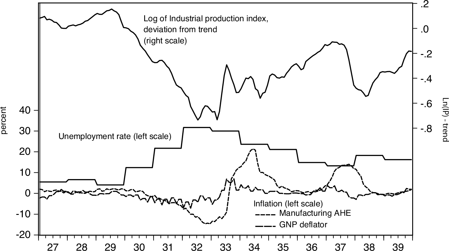
Figure 1 plots series that indicate the course of real activity and inflation from the late 1920s through 1939. These particular series for real activity and wage inflation have comparable counterparts in other historical eras: they are constructed in the same way, with no obvious differences in cyclical properties. The unemployment rate is Weir’s (Reference Weir1992) “private nonfarm” unemployment rate, which runs from 1890 through 1990.Footnote 1 Like other comprehensive unemployment estimates for the 1930s, it is only available annually. To indicate real activity at a monthly frequency, I plot the Federal Reserve Board’s seasonally-adjusted index of industrial production (IP), expressed as the deviation of the log from a linear trend between benchmark years following Romer (1989) and Balke and Gordon (1989).Footnote 2 The resulting “IP gap” is consistent with Weir’s unemployment series (over 1929–39, the correlation between the annual average IP gap and Weir’s unemployment series is –0.95) and with the conventional view that real activity remained somewhat depressed throughout the 1930s.
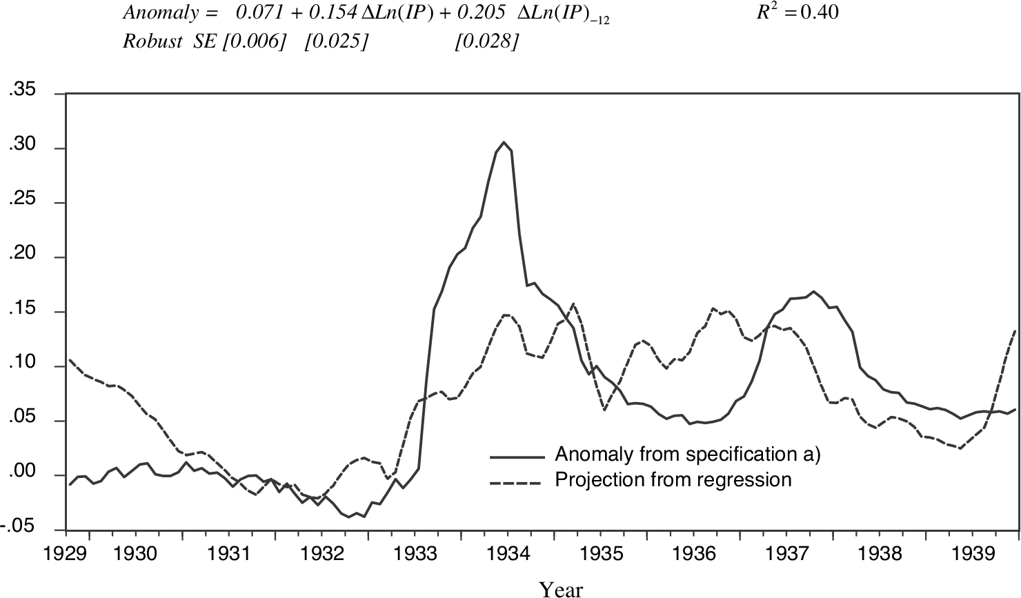
UNEMPLOYMENT RATE (ANNUAL), IP (SA, MONTHLY), 12-MONTH INFLATION IN MANUFACTURING AHE (MONTHLY), AND GNP DEFLATOR (QUARTERLY) 1927–1939
Sources: Unemployment rate, private nonfarm is from Weir (1992). IP index is the Federal Reserve Board Index of IP taken from Federal Reserve Bank of St. Louis FRED (https://fred.stlouisfed.org/series/INDPRO). Manufacturing AHE is from Hanes (1996). GNP deflator is from Balke and Gordon (1986, appendix table 2).

The only time series from the 1920s–1930s that indicate wage inflation and have comparable counterparts in other eras are AHE by industry, for manufacturing only, originally collected by the National Industrial Conference Board (NICB) and the U.S. Bureau of Labor Statistics (BLS). They are available monthly, starting in July 1922. Figure 1 plots the 12-month percent change in an average with fixed industry weights constructed by Hanes (Reference Hanes1996), which continues into the post-WWII era.Footnote 3 Of course, the AHE series are an imperfect indicator of movements in wage rates. I will return to this issue later. The figure shows manufacturing AHE inflation was close to zero in the late 1920s. It started to fall (which meant deflation) almost immediately after the 1929 cyclical peak, generally dated in October 1929. It began to rise again in late 1932, shortly after the cyclical trough dated by Romer (1994) in July 1932 (the NBER dated it in March 1933). From late 1933 through early 1934, AHE inflation rose to extremely high rates, then fell, then rose again in late 1936. It remained high through 1937 while the economy entered a short but sharp recession from a cyclical peak dated in August 1937 (Romer 1994) or May 1937 (NBER). For price inflation, the figure plots the four-quarter percent change in Balke and Gordon’s (1986) quarterly GNP deflator. This follows a path similar to AHE inflation, falling over 1929–33, turning up in late 1932, high in late 1933-early 1934 and 1936–37. A complete account of the path of price inflation in the 1930s is beyond the scope of this paper. My focus is on wage inflation. But it should be clear from the figure that causes of anomalous movements in wage inflation, if they can be identified, may also account for much of the high price inflation of the 1930s. I will return to this point later.
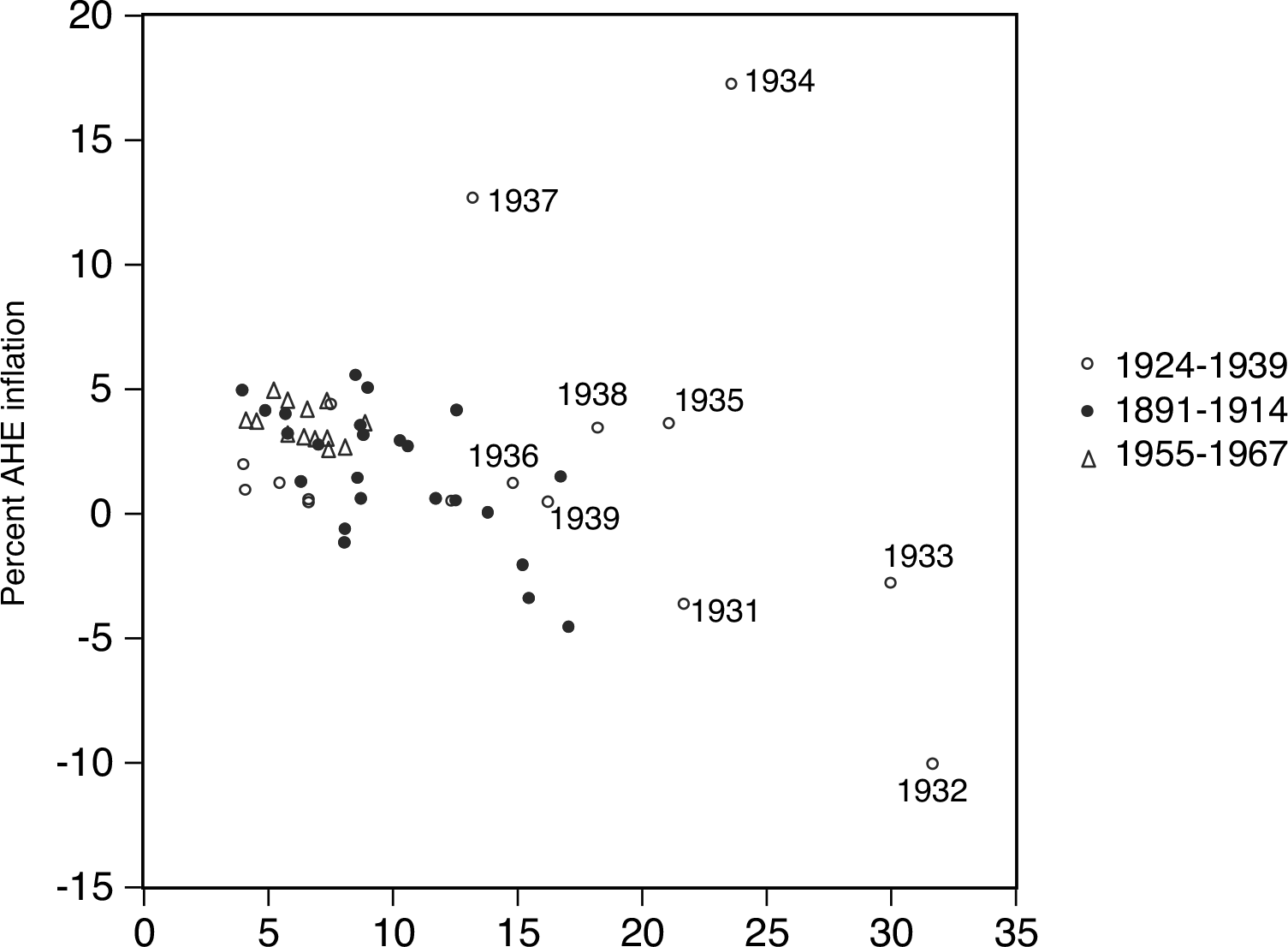
Samuelson and Solow (1960) observed 1930s wage inflation anomalies in a simple scatterplot of wage inflation against unemployment, with observations from the 1920s–30s placed alongside data from other eras of American history. I start the same way, but I must keep in mind a change in the nature of the Phillips curve in the late 1960s. American data from the pre-1914 era, the 1920s, and the early post-WWII era show a positive relationship between real activity and inflation (a negative relationship with unemployment rates) like the original pattern found by A.W. Phillips (Reference Phillips1958). Later a different pattern appears: the “accelerationist Phillips curve,” a positive relationship between real activity and the change in inflation from the prior year. The shift is generally observed to have occurred between 1966 and 1970 (e.g., Gordon Reference Gordon1972; King and Watson 1994). Recently many economists have observed a shift away from the accelerationist Phillips curve back to a relationship of the original form (Gali Reference Gali2011; Kiley Reference Kiley2015; Blanchard Reference Blanchard2016; Ball and Mazumder Reference Ball and Mazumder2019), but the timing of this later shift is less clear; it is variously dated from “around the mid-1980s” (Gali Reference Gali2011, p. 451) to “around 2000” (Ball and Mazumder Reference Ball and Mazumder2019).
Figure 2 scatters the percent change in the annual average value of manufacturing AHE series against annual unemployment rates over 1924–39 and two other spans that are generally agreed to have followed the original Phillips curve relationship: 1891–1914 and 1955–1967. All of these spans are covered by Weir’s (Reference Weir1992) unemployment rate series. The years 1955–1967 are covered by a continuation of the manufacturing AHE series for the 1920s–30s. The years 1891–1914 are covered by a manufacturing AHE series that is at least roughly comparable.Footnote 4 Beginning the postwar sample in 1955 avoids years directly affected by the Korean War wage and price controls (lifted in February 1953 (Rockoff Reference Rockoff1984)). Note that wage inflation over 1929–1932 is in line with the Phillips curve prevailing in the other eras. The outliers—the anomalies—are 1933–35 and 1937–38.
ANNUAL UNEMPLOYMENT RATE AND INFLATION IN MANUFACTURING AHE, 1891–1914, 1924–1939, 1955–1967
Sources: Unemployment rate, private nonfarm, is from Weir (1992). AHE 1924–1939 and 1955–1967 is from Hanes (1996). AHE 1891-1914 is from Rees (1961, table 21) “Nine industries combined.”

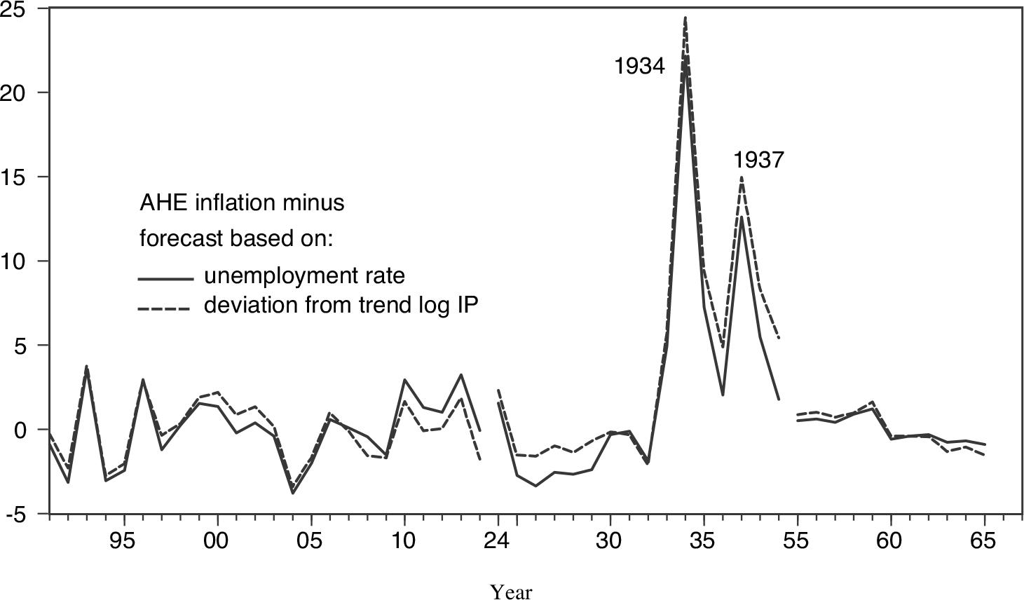
Figure 3 shows the anomalies in a different way. For this figure, I regressed AHE inflation 1891–1914 and 1955-67 on the current and previous years’ unemployment rate and a dummy variable for pre-WWII years. I also ran the regression with the unemployment rate replaced by deviation from trend in IP defined as for Figure 1.5 Results were
(** denotes significantly different from zero at 1 percent level):
AHE inflation = 6.74** – 0.47 Prewar – 0.43** Unemployment – 0.03 Unemployment(–1)
Robust SE [0.93] [0.73] [0.14] [0.15] R 2: 0.49
AHE inflation = 3.74** –2.42** Prewar + 10.79** IP gap – 6.74 IP gap(–1)
Robust SE [0.52] [0.64] [4.15] [4.17] R 2: 0.54
Applying estimated coefficients to real activity series 1929–39 gives “projected” AHE inflation rates. In Figure 3, I plot actual AHE inflation minus projections. Unemployment and IP give the same result: over 1933–35 and 1937–38, actual inflation greatly exceeds projections, far more than in any year, outside that era.
DEVIATION FROM PROJECTED AHE INFLATION, 1891–1914, 1924–1939, 1955–1967
Source: Author's calculations.

PROPOSED EXPLANATIONS FOR ANOMALOUS WAGE INFLATION IN THE 1930S
New Deal Labor Policies
Many economists, in addition to Samuelson and Solow (1960) and Friedman and Schwartz (1963), have ascribed 1930s inflation anomalies to effects of New Deal labor policies. According to Wachter (1976, p.155), “The spurt [in wage inflation] in the early 1930s is generally attributed to the NIRA, and the Wagner Act and the subsequent growth of unions may have been responsible for that of the late 1930s.” Mitchell (Reference Mitchell and Beckerman1986) observes that NRA codes “included labor provisions which boosted wage rates…also provided encouragement to unions and collective bargaining…despite the depth of the depression, a spate of wage increases developed as the codes came into force” (p. 68). Romer (1999) argues that minimum wages and other provisions of NRA codes tended to boost price inflation partly because they stymied the usual effect of high unemployment rates on wage inflation. Weinstein (Reference Weinstein1980) regresses monthly wage inflation in the 1920s–30s sample on a measure of real activity, lagged inflation, and dummy variables to allow for effects of NRA codes; results indicate that the advent of the NRA boosted wage inflation. Gordon (1983, p. 95) runs similar regressions on long samples, including the 1930s, adding dummy variables to allow for effects of “the 1935 Wagner Act.unionization in 1936-37” as well as dummies for NRA years.
Hysteresis, Downward Nominal Wage Rigidity
Both the hysteresis model of Blanchard and Summers (Reference Blanchard and Summers1986) and the DNWR model of Akerlof, Dickens, and Perry (Reference Akerlof, Dickens and Perry1996) were framed in terms of the “expectations-augmented” Phillips curve hypothesized by Phelps (Reference Phelps1967) and Friedman (Reference Friedman1968). This is a relationship between real activity and the spread between current inflation and expectations of current inflation formed in the past, such that current inflation equals expected inflation when real activity is at its “natural rate.” It appears in models where wages and prices are determined by the behavior of agents who lack (or ignore) information about current macroeconomic conditions (e.g., Phelps et al. Reference Phelps, Alchian and Holt1970; Lucas Reference Lucas1972; Mankiw and Reis 2002). It generates an empirical Phillips curve of the original form if the natural rate of unemployment is stable enough, and expected inflation is uncorrelated with recently experienced inflation. It generates an accelerationist Phillips curve if expected inflation is strongly correlated with recent inflation. Many economists have argued that the late-1960s shift in the empirical Phillips curve to the accelerationist form can be accounted for in this way (e.g., Alogoskoufis and Smith 1991; Ball Reference Ball2000). Indeed, there is evidence that the correlation between expected inflation and recent inflation increased across the late 1960s and fell again after the 1980s, consistent with the reappearance of the original-form Phillips curve (e.g., Barsky Reference Barsky1987; Kiley Reference Kiley2015).
In Blanchard and Summers’ (Reference Blanchard and Summers1986) hysteresis model, the natural rate of unemployment is not stable: it is affected by recent employment levels, mainly because workers having bargaining power care little about the welfare of the unemployed. Thus wage inflation can rise as soon as employment begins to recover from a large, persistent recession. In terms of the empirical Phillips curve, wage inflation may be related to recent growth, rather than the current level, of real activity. Blanchard and Summers draw some of their evidence for this proposition from regressions of annual AHE inflation 1920–1941 on a proxy for expected inflation and estimates of the current and previous years’ annual unemployment rates or aggregate employment. The results indicate that across these years, annual AHE inflation was indeed strongly related to growth in real activity. Blanchard and Summers do not discuss New Deal labor policies.
In the DNWR model of Akerlof, Dickens, and Perry (Reference Akerlof, Dickens and Perry1996), wage inflation usually follows a Friedman-Phelps expectations-augmented Philips curve. But wage deflation, which would otherwise result from high unemployment and low expected inflation, can be constrained by a social norm which prevents nominal wage cuts unless the employer is in “financial distress” evidenced by extreme decline in profit. They construct a model of annual inflation in a GDP deflator, having assumed a stable relationship between wage and price inflation. They “show that a dynamic simulation of the model fit to postwar data closely tracks price changes during the Great Depression” (p. 5). In the simulation, the constraint on wage cuts does not bind over 1929–1932, but it binds strongly after that as profits recover, especially in 1933, 1936, and 1939 (pp. 44–47). Like Blanchard and Summers (Reference Blanchard and Summers1986), they do not discuss New Deal labor policies.
The New Keynesian Policy Expectations Mechanism
The new Keynesian Phillips curve (Roberts Reference Roberts1995) appears in models where there is a cost of adjusting nominal wages, prices, or both (as in Rotemberg (Reference Rotemberg1982) and Gertler and Leahy (Reference Gertler and Leahy2008)) or a constraint that prevents adjustment except at certain points in time with “staggering” (as in Taylor (Reference Taylor1979) and Calvo (Reference Calvo1983)). It is a “forward-looking” structural relationship in which current inflation is ultimately determined by two factors. One is the public’s expected value for the long-run future inflation rate, that is, the rate of inflation that will prevail once all predictable deviations of real activity from the natural rate have dissipated (the long-run steady-state inflation rate). The other is the entire expected path of real activity, relative to the natural rate, from the current period to that long-run future point in time. A new Keynesian Phillips curve can generate an empirical Phillips curve of the original form if expected long-run inflation is fixed. It can generate an accelerationist Phillis curve if expected long-run inflation varies and is correlated with recently experienced inflation.Footnote 6 Historical shifts in the empirical Phillips curve can be accounted for in this way. Expected long-run future inflation (like the short-run expectations that matter for the Friedman-Phelps formulation) appears to have been correlated with recent inflation in the late 1960s–1990s, but “anchored” in the pre-1914 era, the early postwar era, and the late 1990s–2000s (Barsky and DeLong 1991; Bordo and Dewald Reference Bordo and Dewald2001; Kozicki and Tinsley Reference Kozicki and Tinsley2001; Mishkin Reference Mishkin2007; Ball and Mazumder Reference Ball and Mazumder2019).
New Keynesian Phillips curve models of wagesetting imply that an empirical Phillips curve relationship can be disturbed by sudden changes in workers’ bargaining power, which create “wage mark-up shocks” (Gali, Smets, and Wouters 2011; Gali Reference Gali2011). Changes in union power are an obvious possible source of such shocks (as noted by Christiano (Reference Christiano2011)). An empirical Phillips curve relationship can also be disturbed by the policy expectations mechanism. Because current inflation is affected by expected long-run future conditions, news that raises the expected long-run future price level can give an immediate boost to current inflation. Thus, the models imply that anomalous wage inflation could have been due to actions of the Roosevelt administration that boosted the expected long-run future price level. Eggertsson (Reference Eggertsson2008) shows that, in a calibrated new Keynesian model, such a change in expectations can cause a surge in inflation and real activity like that in 1933–36. From Eggertsson’s results, it is obvious that the model’s path for inflation relative to real activity would appear anomalous in an empirical Phillips curve.Footnote 7 But Eggertsson does not focus on this point, or on wage inflation specifically.
In Online Appendix 1, I present a general model consistent with many specific new Keynesian settings, in which wage-inflation anomalies of the kind seen in the 1930s result from increases in the expected long-run future price level or wage mark-up shocks. Wage adjustment is subject to a Calvo (Reference Calvo1983) constraint with “indexing” to expected long-run future wage inflation (following Yun Reference Yun1996; Cogley and Sbordone Reference Cogley and Sbordone2008; Coibion, Gorodnichenko, and Wieland 2012). A key assumption, following Gali (Reference Gali2011), is that the public’s forecasts for real-activity variables such as unemployment or output are ordinarily close to simple autoregressive forecasts. This is quite realistic (Chauvet and Potter Reference Chauvet, Potter, Elliot, Granger and Timmermann2013). I derive an expression that corresponds to empirical Phillips curves:
 $$\[\Delta {w_t} = \phi {(\tilde x - \mathop x\limits^{\~n} )_t} + {E_t}\left[ {\Delta {w_{t + T}}} \right] + {\varepsilon _{1t}} + {\varepsilon _{2t}}\]$$
Δwt is the change in the log of the average wage level. is a time series such as an unemployment rate or deviation of IP from a long-run trend that is usually well-correlated with the difference between real activity and the natural rate, but which would fail to account for sudden changes in the natural rate. E t[Δw t+T] is the public’s expected value for long-run future wage inflation. The original empirical Phillips curve appears when E t[Δw t+T] is stable. The accelerationist form appears when E t[Δw t+T] is correlated with recent inflation. For the 1920s–1930s, I assume E t[Δw t+T] was always close to zero. AHE inflation was close to zero prior to the 1929 downturn and, as detailed later, Roosevelt promised to “reflate” prices, that is to restore the pre-Depression price level, not to create permanently higher inflation. ε 1 and ε 2 are possible disturbances creating wage inflation anomalies. ε 1 is positive when there is an extraordinary increase in the public’s forecast for the long-run future price level. ε 2 is positive when there is a sudden increase in the average markup of wages over workers’ opportunity cost of labor.
MONTHLY TIMING AND NATURE OF 1930S WAGE INFLATION ANOMALIES
Which explanation is most consistent with the facts? I begin to answer that question by identifying the timing of the anomalies at a monthly frequency. To do that, I estimate empirical Phillips curves of various forms on monthly postwar series for which there are directly comparable 1930s counterparts: that means the IP gap for real activity, and the manufacturing AHE series described earlier which can be continued up to March 2003.Footnote 8 My goal is not to choose among the specifications but merely to get estimates for the relationship between AHE inflation and IP gaps that are consistent with a wide variety of models, including but not limited to, new Keynesian models. I apply each estimated specification to IP gaps from 1929 through 1939. I compare the resulting projected “normal” paths for AHE inflation with actual inflation. All specifications give similar results.Footnote 9 From 1929 through July 1933, actual AHE inflation is in line with or below projected paths. Anomalously high inflation first appeared in August 1933. From August 1933 through June 1934, AHE inflation soars above projected paths. Then it drops back down toward the projections. Starting in November 1936, AHE inflation again soars above projections.
Next, I compare the path of manufacturing AHE with a unique series from the 1930s that indicates changes in manufacturing wage rates as distinct from AHE. This series shows that the first spell of anomalous AHE inflation, from August 1933 through 1934, mainly reflects an enormous hike in wage rates over August–September 1933, followed by increases in AHE relative to wage rates from September 1933 through May 1934. The second spell of anomalous AHE inflation, from November 1936 to late 1937, reflects another round of hikes in AHE that began in November 1936 and ended around August 1937.
Estimated Phillips Curve Specifications
For all specifications, the dependent variable is the change in log manufacturing AHE from the same month of the previous year, so that I do not have to quantify seasonals in AHE. It would be easy to confuse changes in seasonals with Phillips curve anomalies, and there are a priori reasons to believe seasonals were unstable across the 1930s.Footnote 10 I specify residuals as MA(12) to account for the overlap of disturbance terms between monthly values of 12-month inflation. All specifications include on the right-hand side a weighted average of the last 12 months’ IP deviations from trend defined as for Figure 1.Footnote 11 (Coefficients on additional lags of IP gaps were generally not significantly different from zero.) Weights were estimated by a second-degree polynomial distributed lag. I allowed weights, as well as the coefficient on the weighted average, to differ across specifications. All samples exclude months for which 12-month inflation could be directly affected by wage and price controls.Footnote 12
Specification (a) corresponds most closely to the new Keynesian Phillips curve. Starting from Expression (1) previously, taking a period to be a month, summing across 12 months, and adding a term to the RHS (ε 3) to account for unmodeled factors such as unobservable determinants of the difference between inflation in AHE versus wage rates, gives:
 $$\[{w_t} - {w_{t - 12}} = \phi \sum\limits_{\tau = 0}^{11} {{{(\tilde x - \mathop x\limits^{\~n} )}_{t - \tau }} + \sum\limits_{\tau = 0}^{11} {{E_{t - \tau }}[\Delta {w_{t + T}}] + {e_t}\,where\,{e_t} = \sum\limits_{\tau = 0}^{11} {{{({\varepsilon _1} + {\varepsilon _2} + {\varepsilon _3})}_{t - \tau }}} } } \]$$
To proxy for E[Δw t+T] (the public’s expected value for the long-run future wage inflation rate), I use a quarterly series created for the Federal Reserve Board’s (FRB)/U.S. macroeconomic model, which represents the public’s forecast for the long-run future rate of consumer price inflation.Footnote 13 Several studies (including Fuhrer (Reference Fuhrer2012), Blanchard, Cerutti, and Summers (2015), and Ball and Mazumder (Reference Ball and Mazumder2019)) have used this series to control for expected long-term price inflation in estimated Phillips curves. Here, to control for changes in expected wage inflation, I put the series on the RHS along with a quadratic time trend to allow for trend changes in the spread between expected wage inflation and expected price inflation (real wage growth). Thus, what I estimate is:
 $$\[{w_t} - {w_{t - 12}} = Const. + {\beta _1}\sum\limits_{\tau = 0}^{11} {{a_\tau }{{(IP - \bar I\bar P)}_{t - \tau }} + {\beta _2}\pi _t^e + {\beta _3}T + {\beta _4}{T^2} + {e_t},} \]$$
where πe is the four-quarter average of the inflation forecast series. The sample is the entire 1948–2003 span (excluding wage- and price-control periods).
Specification (b) is a simple Phillips curve of the original form:
 $$\[{w_t} - {w_{t - 12}} = Const. + {\beta _1}\sum\limits_{\tau = 0}^{11} {{a_\tau }{{(IP - \bar I\bar P)}_{T - \tau }} + {e_t},} \]$$
estimated on a sample ending with December 1965, the earliest point anyone dates the shift to an accelerationist Phillips curve.
Specification (c) is an accelerationist Phillips curve estimated over the span from January 1970 (the latest point anyone dates the shift to the accelerationist Phillips curve) to December 1989 (a relatively early date for the shift back to the original-form Phillips curve). The lagged inflation term is a weighted average (estimated by second-degree polynominal distributed lag) of 12 lags of the 12-month change in log AHE:
 $$\[{w_t} - {w_{t - 12}} = Const. + {\beta _1}\sum\limits_{\tau = 0}^{11} {{a_\tau }(IP - \bar I\bar P} {)_{t - \tau }} + {\beta _2}\sum\limits_{\tau = 0}^{11} {{b_\tau }({w_{t - 12 - \tau }} - {w_{t - 24 - \tau }}) + {e_t}} \]$$
Specification (d) is an accelerationist Phillips curve with lagged wage inflation replaced by lagged price inflation:
 $$ \Delta {w_t} = Const. + {\beta _1}\sum\limits_{\tau = 0}^{11} {{a_\tau }{{(IP - \bar I\bar P)}_{t - \tau }}} \\
+ {\beta _2}\sum\limits_{\tau = 0}^{11} {{b_\tau }({p_{t - 12 - \tau }} - {p_{t - 24 - \tau }}) + {e_{t,}}} \\
$$
where p is the log of the PCE price index. Specifications (e) and (f) are accelerationist Phillips curves estimated over the entire available sample (excluding wage and price control periods), that is, 1948–2003 for lagged wages and 1961–2003 for lagged prices (the PCE price index began in 1959).
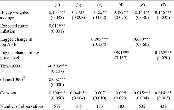
Table 1 gives estimated coefficients from all specifications.
EMPIRICAL PHILLIPS CURVES ESTIMATED ON POST-WWII DATA

Notes: Standard errors in parentheses. ***p≤0.01, **p≤0.05,***p≤0.1.
Samples: (a) 1948:1-1950:12, 1954:12-1971:7, 1975:5-2003:3 (b) 1948:1-1950:12,1955:4 - 1965:12 (c) 1970:1-1971:7, 1976:5-1989:12 (d) 1970:1-1971:7, 1976:5-1989:12 (e) 1948:1-1950:12. 1955:5-1971:7, 1976:5-2003:3 (f) 1961:12-1950:12. 1955:5-1971:7, 1976:5-2003:3
Sources: Federal Reserve Board Index of IP is taken from the Federal Reserve Bank of St. Louis FRED (https://fred.stlouisfed.org/series/INDPRO). Manufacturing AHE and inflation forecast are described in the text. PCE price index is taken from Federal Reserve Bank of St. Louis FRED (https://fred.stlouisfed.org/series/PCEPI).
Projections and Anomalies to Be Explained
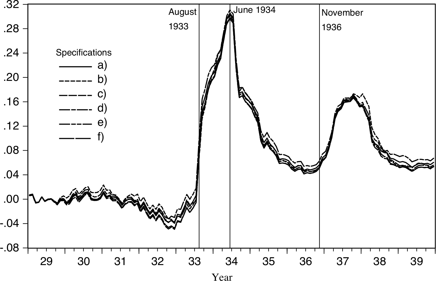
To create projected “normal” paths for inflation in the 1930s, I apply estimated postwar coefficients to actual IP gaps starting with January 1929. I set the other RHS variables to express an assumption that expected the long-run future wage inflation rate remained zero throughout the 1930s. Thus for (a), I set to zero the terms for expected long-run future price inflation and the time trends. For (c)–(f), I set lagged inflation terms to zero. For all specifications, I adjust constants so that projections match actual average inflation from January through September 1929, just prior to the cyclical peak. Thus the projections are meaningful, starting with October 1929. The “AHE inflation anomaly” defined by a specification is actual AHE inflation minus the projection. Figure 4 plots all the resulting anomalies. The timing and relative magnitudes of the anomalies from month to month are very similar across all the specifications. This is true even though weights on IP lags were allowed to vary across specifications. I use Specification (a) (derived from a new Keynesian model) as my benchmark in the figures and results I present later. But results were similar using the anomalies from the other specifications.
AHE INFLATION ANOMALIES, OCTOBER 1929–DECEMBER 1939
Source: Author's calculations.
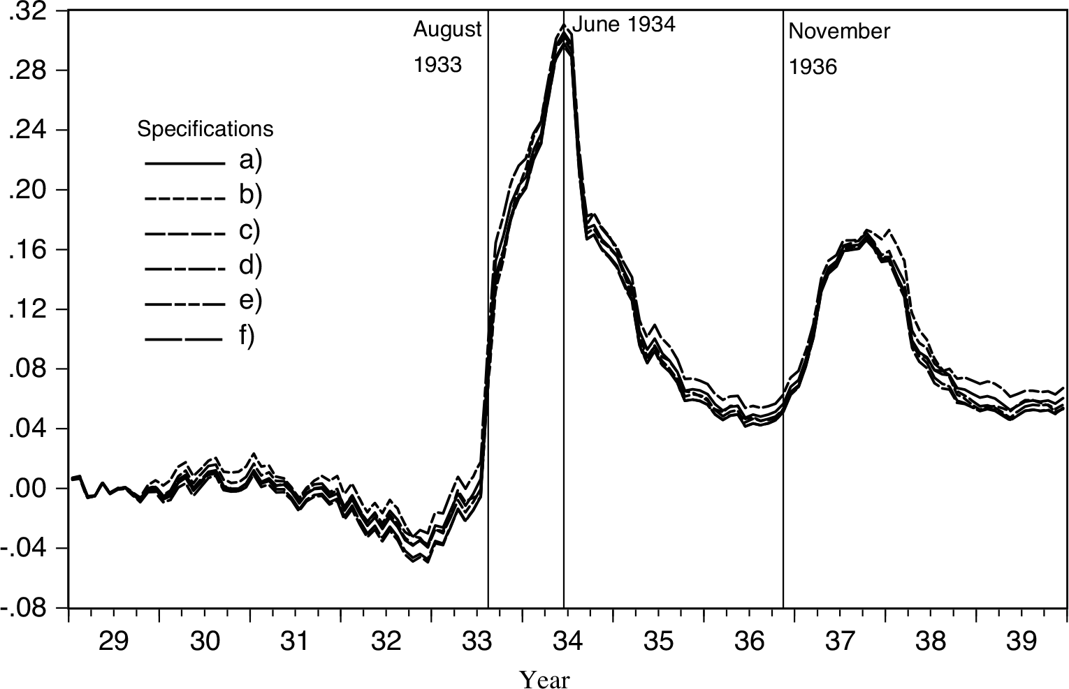
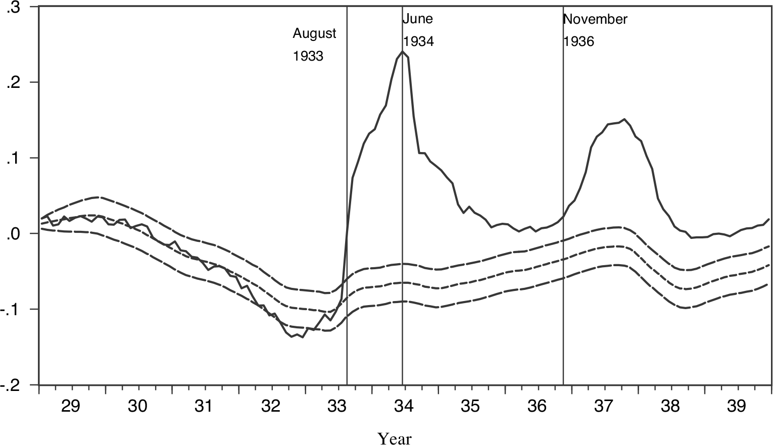
Figure 5 plots the projected path from Specification (a) with two-SE bands, along with actual AHE inflation. Online Appendix 2 plots projected paths with two-SE bands for (b)–(f). From late 1929 through early 1932, actual inflation remains within the two-SE bands of all projections. In 1932 and early 1933, actual inflation falls below projections. Starting in August 1933, actual inflation soars far above all of the projections. Thus I take August 1933 to be the month when AHE inflation first became anomalously high. The largest difference between actual inflation and projected paths appears over the 12-month span ending June 1934. After that, the difference narrows. By mid-1936, actual 12-month inflation is much closer to projections although still above the two-SE bands. Starting in November 1936, inflation again soars above the projected paths, peaking in the 12 months ending October 1937. Then actual inflation falls back toward projections. All of these patterns are consistent with the results from annual data on IP or unemployment in Figure 3.
PROJECTED AHE INFLATION FROM SPECIFICATION (A) WITH TWO-SE BANDS (A)
Source: Author's calculations.

Movements in Wage Rates versus AHE
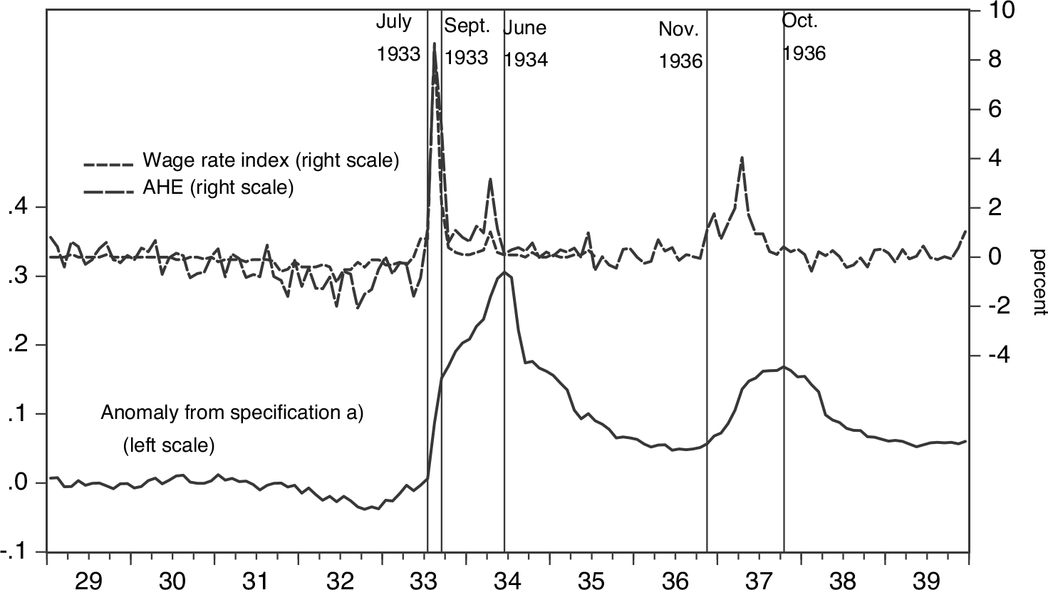
The AHE series I use here, even with fixed industry weights, could be affected by many factors in addition to changes in wage rates: relative employment at high- versus low-wage rates within industries, changes in the prevalence and nature of piece rates, or overtime premiums. A unique series from the 1930s indicates changes in manufacturing wage rates per se. From the early 1920s through October 1935, the BLS asked respondents to its monthly survey of manufacturing establishments to report changes in wage rates—piece as well as time rates—and the number of employees affected by each change. From published summaries of these reports, Creamer (Reference Creamer1950) constructed a “wage rate index.” Changes in the index number indicate average changes in straight-time or piece-rate wages paid for nonmanagerial jobs in reporting establishments (averaging in zeros for jobs in which wages were held fixed). The index has a number of shortcomings. It may fail to indicate small monthly changes in average wage rates.Footnote 14 There are no comparable data for months subsequent to October 1935 or from other eras. But it is the only high-frequency indicator of changes in wage rates, as distinct from AHE, in a large sample of manufacturing establishments in the 1930s.
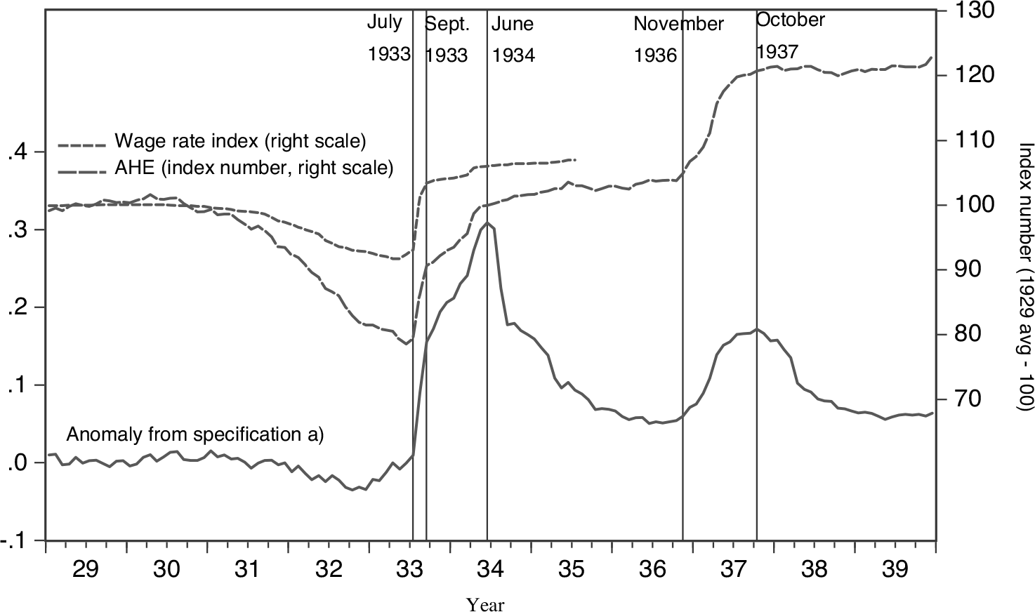
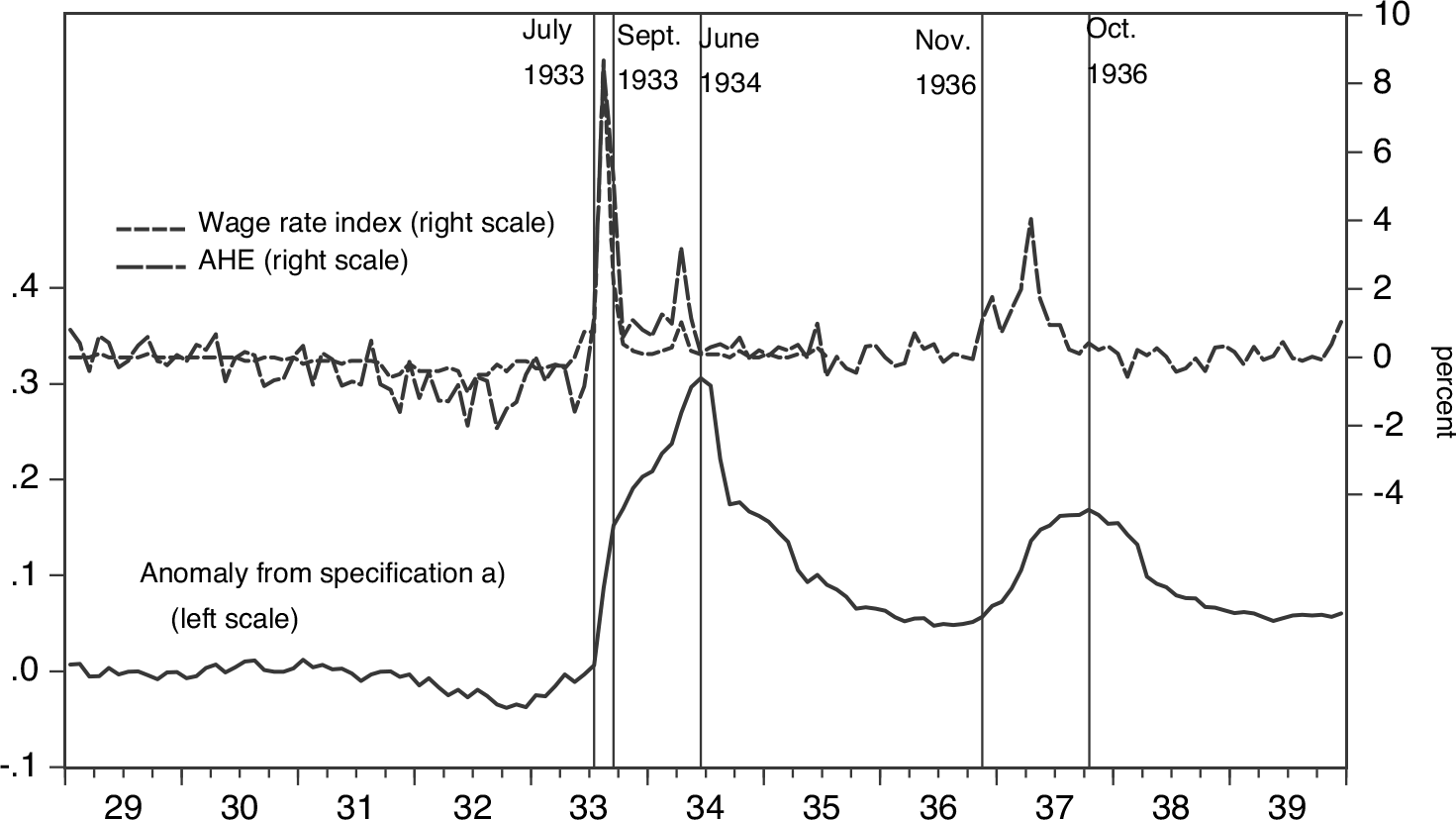
Figure 6 plots the wage rate index and the manufacturing AHE series alongside the inflation anomaly defined by Specification (a). Figure 7 plots monthly percent changes (not 12-month inflation). The figures show that the spell of anomalous AHE inflation beginning in August 1933 was at first due to wage hikes in August and September 1933 (the increase from July to September observations was 14 percent in AHE, 11 percent in the wage rate index). From September 1933 through spring 1934, anomalous inflation mainly reflects growth in AHE relative to wage rates (from September 1933 to May 1934 AHE increased about 10 percent, the wage index just about 2 1/2). AHE grew slowly from May 1934 to November 1936, then very rapidly again from November 1936 to October 1937, fastest in April 1937.
LEVELS OF AHE SERIES AND WAGE RATE INDEX, AHE INFLATION ANOMALY
Sources: AHE is index number calculated from Hanes (1996). Wage rate index is from Creamer (1950, table A). Anomaly is from the author's calculations.

MONTH-TO-MONTH PERCENT CHANGES IN AHE AND WAGE RATE INDEX, AHE INFLATION ANOMALY
Sources: AHE is from Hanes (1996). Wage rate index is from Creamer (1950, table A). Anomaly is from the author's calculations.
WHAT BEST EXPLAINS THESE MOVEMENTS IN WAGES AND AHE?
So far, I have shown that accounting for 1930s wage inflation anomalies means accounting for large wage hikes in August and September 1933, increases in AHE relative to wage rates from September 1933 through May 1934, and a second round of AHE hikes that began in November 1936 and ended around August 1937. Neither the DNWR model of Akerlof, Dickens, and Perry (Reference Akerlof, Dickens and Perry1996) nor the hysteresis model of Blanchard and Summers (Reference Blanchard and Summers1986) can do this. In the former model recovering profits could reactivate a DNWR constraint that would block nominal wage cuts. But the inflation anomalies reflect massive hikes in wages or AHE. The latter model implies wage inflation could pick up as soon as employment began to grow steadily even if unemployment remained high relative to pre-Depression levels. It cannot explain why wage growth occurred in such sudden leaps across August–September 1933 and after November 1936.
That leaves New Deal labor policies and the new Keynesian policy expectations mechanism, which I examine in the remainder of this section. I find the wage hikes of August–September 1933 coincided with the effective dates of the first NRA codes. The changes in wage rates required by the provisions of those codes appear to account for the magnitude of movements in manufacturing wages and AHE across those months. Increases in AHE relative to wage rates from September 1933 to April 1934 coincided with the spread of NRA industry codes, which did not further raise wage minimums but did impose labor standards such as premium pay for overtime, which would tend to raise AHE relative to straight-time wages. Hikes in AHE from November 1936 to October 1937 coincided with a wave of strikes associated with unionization supported by New Deal labor policies. Many employers raised wages and overtime premiums as they entered into agreements with unions or attempted to forestall union threats. Overall, the first NRA codes in August–September 1933, the spread of NRA industry codes from September 1933 through May 1934, and union activity indicated by strikes, appear to fully account for AHE inflation anomalies over 1933–39.
Turning to the expectations mechanism, I find that the wage hikes of August–September 1933 coincided with policy news that could have raised the expected long-run future price level. But other, apparently similar news came in months prior to August 1933, when inflation was not anomalously high. The second round of extraordinary hikes in AHE from November 1936 to October 1937 cannot possibly be accounted for by the policy expectations mechanism. It occurred in the midst of events that should have, if anything, lowered the expected future price level.
New Deal Labor Policies
The NIRA was passed in June 1933. In July 1933, the NRA approved the first three industry codes, for cotton textiles, woolen textiles (both covered in my manufacturing AHE series), and shipbuilding (not covered). All three codes hiked wages of all workers by requiring universal cuts in weekly hours with no cuts in weekly pay and set industry-specific wage minimums. The cotton and shipbuilding codes required employers to raise wages in higher-paid jobs to maintain differentials over jobs that had previously been paid below the new minimums.Footnote 15
In late July 1933, Roosevelt “invited” nearly all nonagricultural employers in other industries to sign the “President’s Re-Employment Agreement” or “blanket code” to regulate employment until their own industry codes were approved. The blanket code forbade wage cuts for any workers and imposed wage minimums.Footnote 16 It called for hikes in wages above the minimum “by an equitable readjustment of all pay schedules.”
The effective dates of the blanket code and the first industry codes were precisely coincident with the extraordinary increases in the manufacturing AHE series in August and September 1933.Footnote 17 It is plausible that these codes were responsible for most, perhaps all, of the 14 percent increase across those months. For four industries covered by the AHE series, NRA staff estimated the direct effect of the industry or blanket code minimums, based on information no longer available. The estimates imply percent increases in industry average wages or AHE ranging from 10 to 30 percent.Footnote 18 According to contemporary observers, wages in higher-paid jobs were, in fact, usually raised when, or shortly after, minimums came into force (Lyon et al. Reference Lyon, Homan, Lorwin, George, Dearing and Marshall1935, p. 318; Roos Reference Roos1937, p. 193). In cotton and woolen textiles, just the code provisions that required cuts in weekly hours with no cuts in weekly pay implied 20 percent hikes in hourly wages.Footnote 19
Beginning in September 1933, most industries adopted their own industry codes.Footnote 20 Like the first round of codes, these codes banned wage cuts for any workers, set wage minimums, and had clauses requiring maintenance of wage differentials for higher-paid workers. But the minimum wages they specified were usually no higher, and sometimes lower, than those already in the blanket code.Footnote 21 On the other hand, nearly all of these later codes required overtime premium pay, which had not been required by the blanket code or the first three industry codes (which were later revised to require overtime pay) (Schoenfeld Reference Schoenfeld1935, p. 575). Thus, it is plausible that the industry codes coming into effect beginning in September 1933 affected AHE more than wage rates.
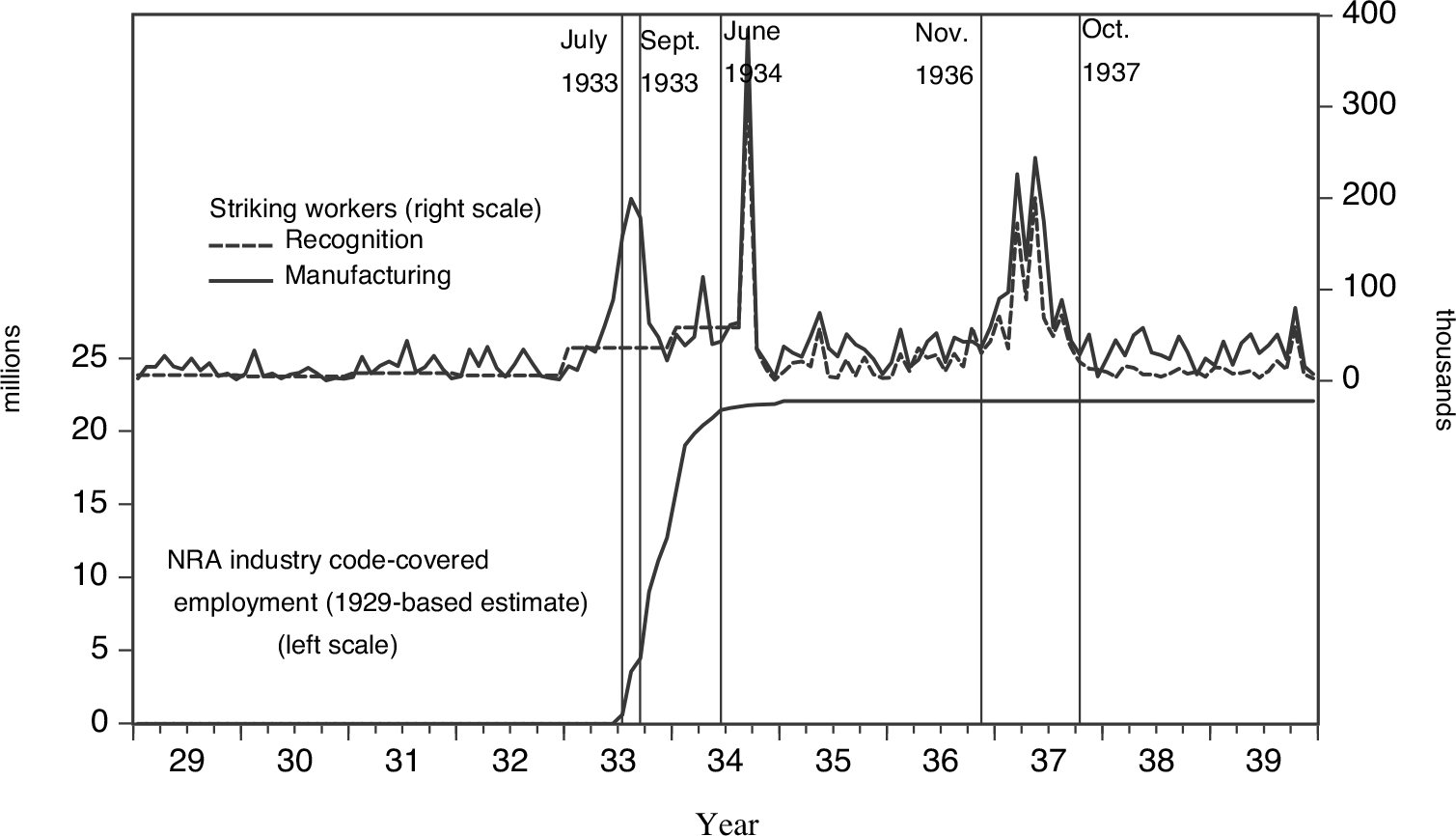
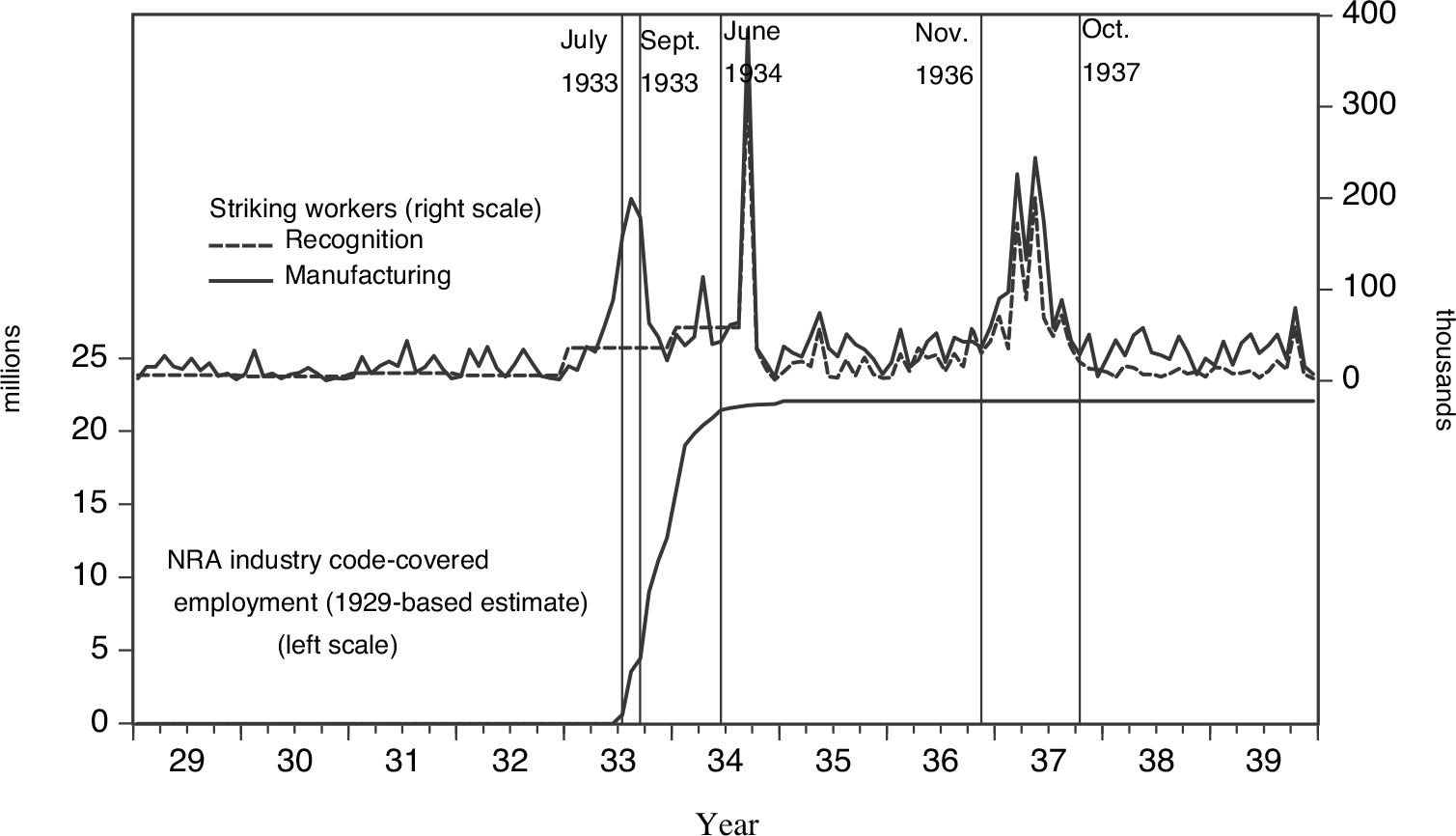
Adoption of these later industry codes was precisely coincident with growth in AHE relative to wage rates from September 1933 to April 1934. This is shown in Figure 8, which plots a monthly estimate of the number of workers covered by industry codes (not including the blanket code) prepared by NRA staff.Footnote 22 It shows that industries representing the bulk of employment adopted their codes between September 1933 and March 1934. The last codes covering industries within my manufacturing AHE series probably came into effect just before the April 1934 AHE observation.Footnote 23
EMPLOYMENT IN INDUSTRIES COVERED BY NRA INDUSTRY CODES, WORKERS INVOLVED IN STRIKES BEGINNING IN MONTH
Sources: NRA code-covered employment is from United States National Recovery Administration (1935, exhibit II, p. 45). Strike series are described in the text.
Apart from the wage and labor-standard provisions of NRA codes, the NIRA and subsequent New Deal policies boosted union bargaining power. When Roosevelt entered office, few American employers, and none in large-scale manufacturing industries, regularly negotiated with unions. Many employers routinely fired employees for union involvement.Footnote 24 The NIRA required every NRA industry code to include a provision “That employees shall have the right to organize and bargain collectively through representatives of their own choosing, and shall be free from the interference, restraint or coercion of employers.no employee.shall be required as a condition of employment.to refrain from joining, organizing or assisting a labor organization of his own choosing.” Contemporaries observed that “The fear of employers which had long kept workers from joining trade unions was for the time being overcome” (Lyon et al. Reference Lyon, Homan, Lorwin, George, Dearing and Marshall1935, p. 489). Unions immediately began membership drives in “Feverish efforts at organization” (MacDonald, Palmer, and Wolfson 1934, p. 13; see, also, Wolman Reference Wolman1936, pp. 59–61; Roberts Reference Roberts1944, p. 95; Bernstein Reference Bernstein1969, pp. 37–38; Fine 1969, p. 66; Rose Reference Rose1997, p. 98).
A wave of strikes accompanied the unionization drives (MacDonald, Palmer, and Wolfson 1934, p. 16; Bernstein Reference Bernstein1969, pp. 96, 99, 106). “Some of these strikes were strategic maneuvers undertaken by the unions to influence the formulation of the labor provisions of the codes…Others were primarily strikes for union ‘recognition’.” (Lyon et al. Reference Lyon, Homan, Lorwin, George, Dearing and Marshall1935, p. 490). In a “recognition” (or “organizing”) strike, one of the union’s demands was that the employer negotiate with the union and stop firing workers for union involvement. “In most of these cases other matters, especially wages, were also major issues” (BLS Monthly Labor Review January 1936, p. 161). Some employers responded to strikes by recognizing unions and raising wages (Fine Reference Fine1963, p. 208; Bernstein Reference Bernstein1969, pp. 217–317, 226, 228, 250). Others raised wages but refused to recognize a union (MacDonald, Palmer, and Wolfson 1934, pp. 41–42; Roos Reference Roos1937, p. 215; Fine Reference Fine1963, pp. 105, 125). Many set up employer-controlled “Employee Representation Plans” (ERPs or “company unions”) to serve as the collective bargaining representative called for by the NIRA (Brooks Reference Brooks1940, p. 75; Roberts Reference Roberts1944, pp. 100–104; Ozanne Reference Ozanne1967, p. 146; Rose Reference Rose1997, p. 115), and gave wage increases “negotiated” with the ERP to draw employee support away from outside, independent unions (Brooks Reference Brooks1940, p. 99; Rose Reference Rose1997, pp. 163, 236; Ozanne Reference Ozanne1967, pp. 147– 149). Employers continued to fire employees involved with unions (Roos Reference Roos1937, p. 233; Lyon et al. Reference Lyon, Homan, Lorwin, George, Dearing and Marshall1935, p. 490) and generally ignored, or tied up in court, rulings of the National Labor Relations Board (NLRB), which had been set up to enforce the NIRA’s collective bargaining provisions (Lyon et al. Reference Lyon, Homan, Lorwin, George, Dearing and Marshall1935, pp. 482–486; Roos Reference Roos1937, pp. 223–226; Rose Reference Rose1997, pp. 123, 137). In May, 1935 the Supreme Court ruled that the NIRA was unconstitutional.
Just two months later, in July 1935, Roosevelt and the Democrats passed the Wagner Act (National Labor Relations Act). The Wagner Act reinstated and strengthened the NIRA’s labor provisions. It banned ERPs and gave the NLRB power to enforce its rulings in federal court (Bernstein Reference Bernstein1969, pp. 322–330). However, employers continued to litigate against, or simply ignore, NLRB rulings. They believed Roosevelt and the Democrats were going to lose the election of 1936, in which case the Wagner Act would be eliminated, or the Supreme Court would rule the Wagner Act, like the NIRA, unconstitutional (Ozanne Reference Ozanne1967, p. 151; Fine 1969, p. 182; Rose Reference Rose1997, p. 240).
In November 1936, Roosevelt was re-elected, and pro-union Democratic governors were elected in several industrial states. There was a second wave of union membership drives and strikes (BLS Monthly Labor Review May 1937; Slichter Reference Slichter1938, p. 98; Fine 1969), including “sit down strikes” (a type of strike later ruled illegal by the Supreme Court (Bernstein Reference Bernstein1969, p. 678)). This second strike wave resulted in an unprecedented increase in union power. By the end of March 1937, employers in large-scale manufacturing industries, including automobiles, steel, chemicals, electrical equipment, and rubber, had recognized unions and entered into written agreements. The agreements usually involved immediate pay hikes and more generous overtime provisions (Bernstein Reference Bernstein1969, pp. 464–468, 481–620; Fine 1969, pp. 302–328, 464–68; Rose Reference Rose1997, p. 258). In April 1937, the Supreme Court ruled the Wagner Act constitutional. From April through September 1937, “Wage rates were influenced by the large number of industrial disputes and by the efforts of employers to forestall unions by making concessions” (Slichter Reference Slichter1938, p. 99). Annual union density estimates show an enormous increase from 1936 to 1937 (Freeman Reference Freeman, Michael, Goldin and Eugene1998). Recognition strikes became rare as NLRB-overseen elections became the mechanism by which unions won recognition (Bernstein Reference Bernstein1969, p. 788).
It is plausible that the process of unionization over 1933–38 would be associated with anomalies in Phillips curves. The wage hikes that employers gave as they entered into union agreements or attempted to forestall union threats were large. They occurred while real activity was still depressed. A relationship between unionization and Phillips-curve anomalies is also consistent with new Keynesian models. As noted previously, and illustrated in Online Appendix 1, new Keynesian models of wage inflation imply that sharp increases in workers’ bargaining power can create anomalies in the usual relation between wage inflation and real activity.
Figure 8 shows the monthly timing of the two strike waves. It plots BLS estimates of the number of workers involved in strikes beginning in a given month, in manufacturing industries specifically, and in recognition strikes in all industries. The latter series begins with September 1934; I link it to annual estimates of workers in recognition strikes, which start earlier, converted to a monthly rate.Footnote 25 Unfortunately, the BLS never published estimates for recognition strikes in manufacturing specifically. The figure shows that the first strike wave began immediately upon passage of the NIRA in June 1934, and ebbed by late 1934. The second wave began in November 1936 and ended in late 1937. It appears that many manufacturing strikes in the second wave were recognition strikes, as the two series fluctuate together.
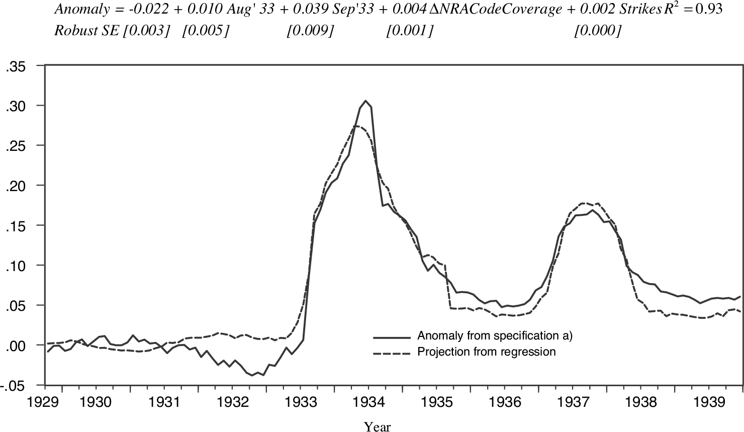
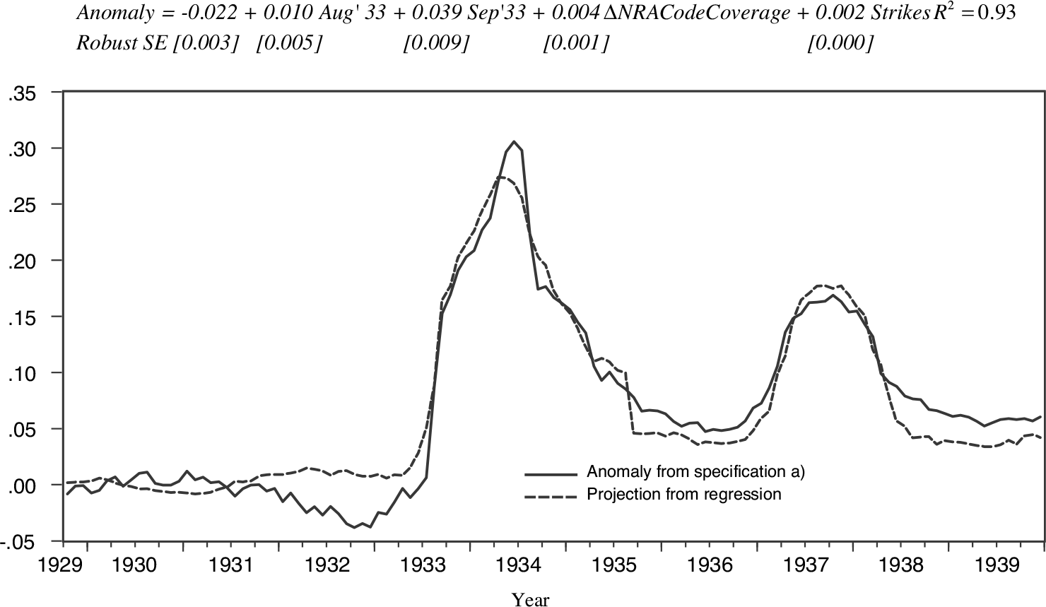
Comparing Figure 8 with Figures 4–6, one sees that the strike wave from late 1936 to late 1937 was precisely coincident with the growth of AHE from November 1936 to October 1937, which constitutes the second anomaly in AHE inflation. In fact, practically all anomalous inflation in manufacturing AHE that was not coincident with the advent of the first NRA codes (August–September 1933) or with the spread of later NRA industry codes (September 1933 through May 1934) was correlated with strikes in manufacturing. This is shown in Figure 9. The upper portion of the figure gives results of regressing the 12-month AHE inflation anomaly defined by Phillips curve Specification (a) on three right-hand side variables: the number of manufacturing workers involved in strikes, averaged over the past 12 months; the 12-month change in NRA-code covered employment; and dummies marking 12-month spans containing August 1933 or September 1933. The lower portion of the figure plots the anomaly “projected” by the estimated coefficients. Because of the way the inflation anomaly is defined, the standard errors of this regression should not be interpreted in the ordinary way. But the R 2, 0.93, does show that the fit between the projection and the anomaly is close. The figure also shows that the projection is close to the actual inflation anomaly throughout the 1930s. It reproduces not only the rise of anomalous inflation in 1933 but also the dimunition of anomalous inflation in 1936 and the second round of anomalous inflation in late 1936–1937.
AHE INFLATION ANOMALY AND PROJECTION ON MEASURES OF THE NEW DEAL LABOR POLICIES
Sources: NRA code-covered employment is from the United States National Recovery Administration (1935, exhibit II, p. 45). Series on workers involved in manufacturing strikes is described in text. Author's calculations.
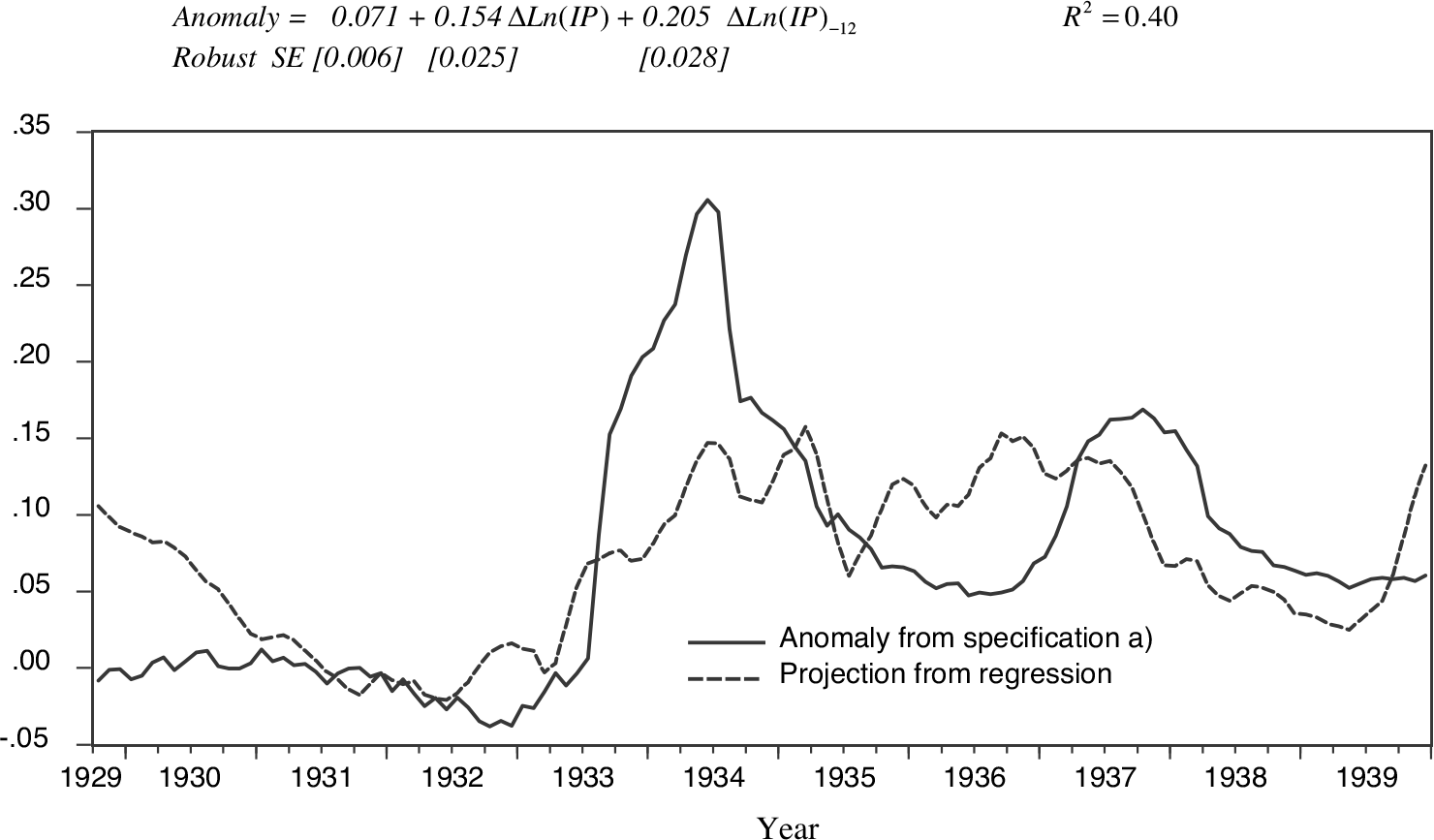
An alternative explanation of 1930s wage inflation, the hysteresis model of Blanchard and Summers (Reference Blanchard and Summers1986), can be subjected to the same test. It does not fare nearly as well. Recall this model implies a relationship between wage inflation and growth in real activity. Figure 10 shows the results of regressing the anomaly defined by Specification (a) on the 12-month change in the log of IP and the previous year’s 12-month change. (Note that this exercise looks for an extra rate-of-growth present in the 1930s: any rate-of-growth effect also present in the postwar period is already built into the postwar coefficients used to define the inflation anomaly.) There was indeed a correlation between the inflation anomaly and recent output growth, but this can only account for an anomalous increase in inflation over 1933–34. It cannot account for the concentration of wage growth in August–September 1933, the dimunition of anomalous inflation in 1936, or the increase in anomalous inflation in late 1936.
AHE INFLATION ANOMALY AND PROJECTION ON RECENT GROWTH OF IP
Sources: IP index is the Federal Reserve Board Index of IP taken from the Federal Reserve Bank of St. Louis FRED (https://fred.stlouisfed.org/series/INDPRO) and author's calculations.
The New Keynesian Expectations Mechanism and Roosevelt’s Monetary Policies
In new Keynesian models, anomalously high wage inflation can be caused by credible news about economic policy that raises the public’s expected value for the long-run future price level. Arguably, such news came thick and fast soon after Roosevelt took office in March 1933.
Entering the Great Depression, currencies of most countries active in international trade and finance could be freely exchanged for gold at a fixed rate, creating the international gold standard. A country’s long-run equilibrium price level was largely determined by its currency’s “gold price,” that is, its exchange rate against gold, and the world gold price level of tradable goods. In the United States, the Federal Reserve system was legally required to exchange its notes and Federal Reserve bank balances for gold at a fixed price. Economists and business writers assumed the dollar gold price would remain fixed in the future and forecast a stable or slightly decreasing U.S. price level based on the balance of world gold supply and demand (Nelson Reference Nelson1991, pp. 6–7).
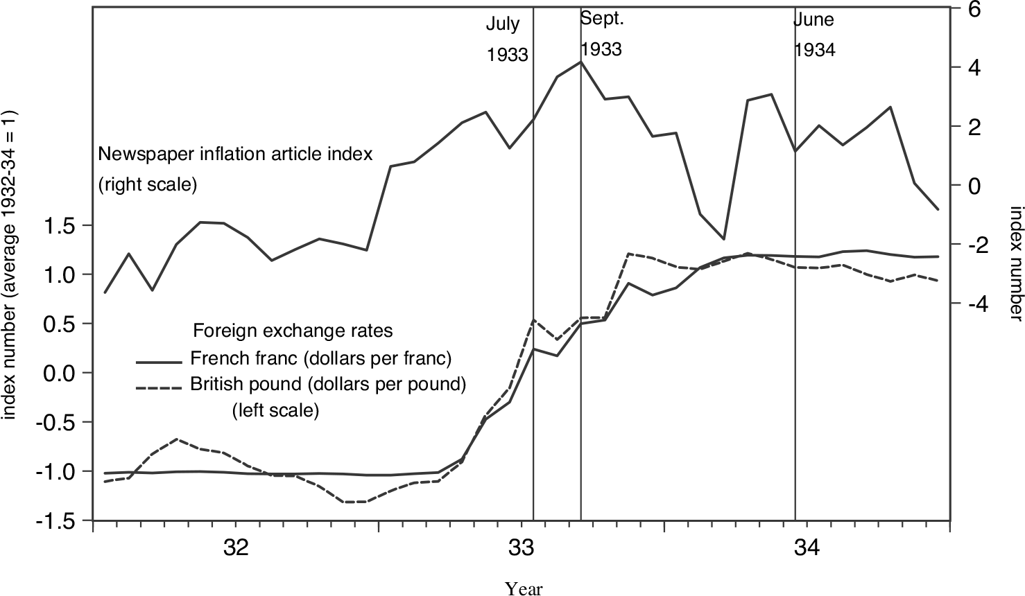
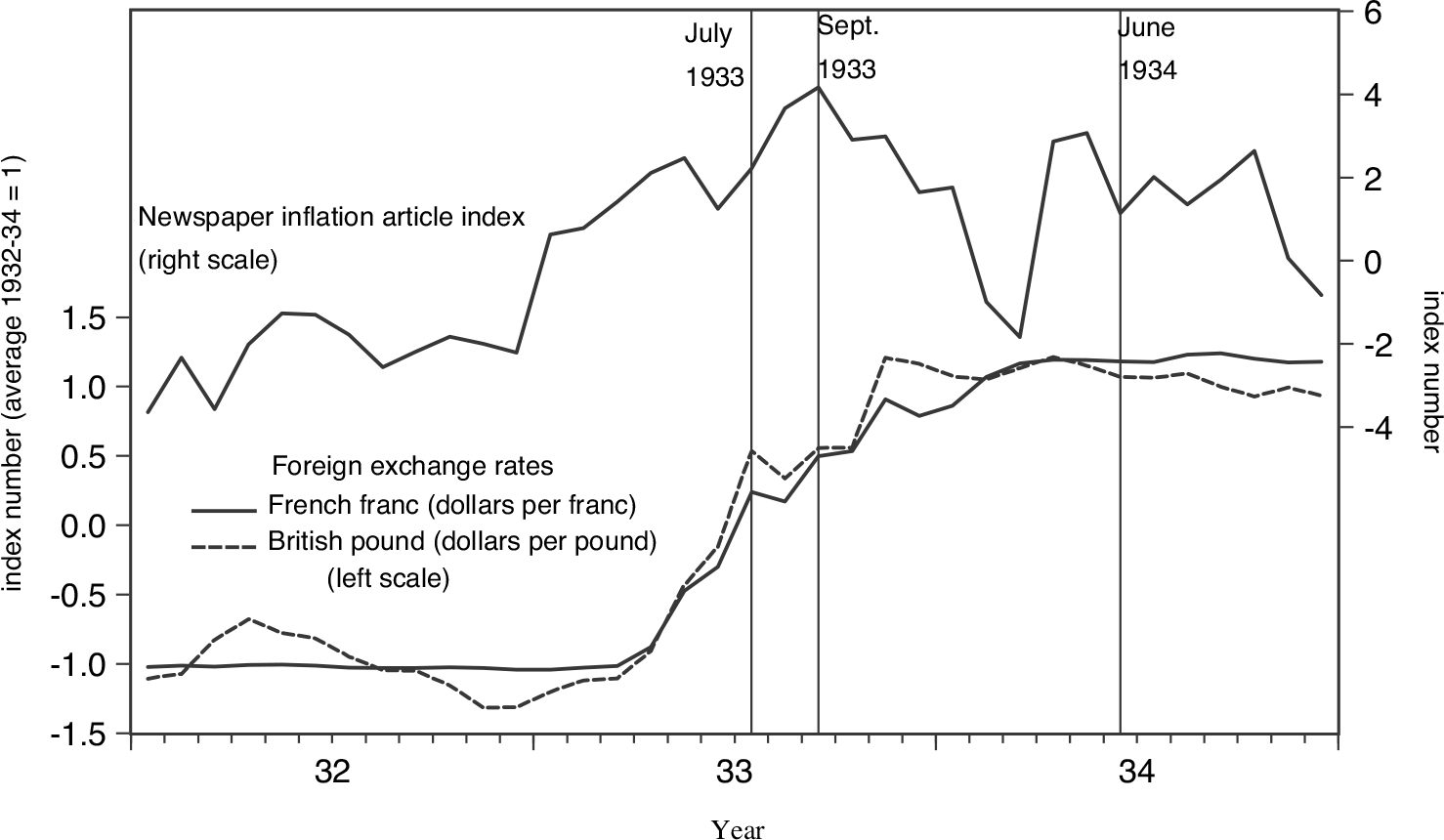
In March 1933, foreign withdrawals of gold from the Federal Reserve system forced Roosevelt to suspend gold payment by the Federal Reserve. For several weeks dollar exchange rates against foreign currencies remained stable, suggesting that market participants expected a quick return to gold payment at the old price. (In the past, many countries, including the United States, had suspended gold payment temporarily.) In late April, however, Roosevelt issued an executive order extending the suspension and “made it clear that the administration intended to permit the dollar to depreciate in terms of foreign currencies as a means of achieving a rise in domestic prices” (Friedman and Schwartz 1963, p. 464). The dollar immediately began to depreciate, as shown in Figure 11, which plots dollar foreign exchange rates against the French franc (fixed to gold until late 1936) and the British pound (devalued in 1932 but kept at a tightly controlled gold price over 1933–36).
EXCHANGE RATES AND NEWSPAPER INFLATION ARTICLE INDEX, JANUARY 1932–DECEMBER 1934 (MONTHLY)
Sources: Exchange rates are from the U.S. Federal Reserve Board (1943, table 173). Newspaper inflation article index is from Binder (2016).
In early May, Roosevelt announced in a national radio broadcast (“fireside chat” 7 May 1933) that “The Administration has the definite objective of raising commodity prices to such an extent that those who have borrowed money will, on the average, be able to repay that money in the same kind of dollar which they borrowed.” Also in early May, Congress passed the Thomas amendment to the Agricultural Adjustment Act. The amendment was “explictly directed at achieving a price rise through expansion of the money stock” and “contained a provision authorizing the president to reduce the gold content of the dollar to as low as 50 per cent of its former weight” (Friedman and Schwartz 1963, p. 465). In June 1933, Congress passed legislation abrogating financial contracts that required payment in gold at the old rate. At the beginning of July 1933, Roosevelt publicly disavowed the aims of an international economic conference that had been convened to arrange a general restoration of gold convertibility at 1929 parities (Friedman and Schwartz 1963, p. 469). In late October 1933, Roosevelt stated in another radio broadcast:
I repeat what I have said on many occasions, that the definite policy of the Government has been to restore commodity price levels. The object …has been to make possible the payment of public and private debts more nearly at the price level at which they were incurred…It has been and is also the purpose to prevent prices from rising beyond the point necessary to attain those ends…When we have restored the price level, we shall seek to establish and maintain a dollar which will not change its purchasing and debt paying power during the succeeding generation (Fireside chat, October 22, 1933).
In January 1934, Roosevelt fixed a new permanent gold price, which devalued the dollar about 40 percent relative to its pre-1933 gold price. At the new price, American monetary authorities sold gold to foreign monetary authorities and bought gold from anyone. The United States was back on the gold standard but at a rate which depreciated the dollar against foreign currencies.
It is plausible that Roosevelt’s announcements and exchange-rate policies raised the public’s expected value for the future price level. At the time, influential economists advocated devaluation of the dollar against gold precisely because they believed it would raise the American price level.26 Before the dollar was relinked to gold in January 1934, some warned that Roosevelt’s policies might bring uncontrollable inflation (Romasco Reference Romasco1983, p. 130; Wilcox, Fraser, and Malin 1934, p. 17). In August 1933, a staff economist at the Federal Reserve Bank of New York observed, “The public has apparently learned that discussion of the currency means ‘devaluation’ which means ‘inflation’ ” (quoted in Romasco Reference Romasco1983, p. 95). On the other hand, Roosevelt’s reflationary policies were strongly opposed by Republicans (Romasco Reference Romasco1983, pp. 49–50) who could reverse them if they regained office. Not all economists believed that devaluation meant inflation; some argued that “there is only a minor relationship between the official prices of gold or silver and the general price level” (Paris Reference Paris1938, p. 9).
The first spell of anomalous AHE inflation, starting in August 1933, was coincident with news events that could have raised the expected future price level. But there were also many such news events prior to August 1933. There are no surveys of the public from the 1930s that could be taken to indicate changes over time in inflation expectations.27 But economic historians who have argued that Roosevelt’s policies raised expected inflation generally argue that the shift in expectations took place prior to July 1933. According to Temin and Wigmore (Reference Temin and Wigmore1990, p. 488), “the real change in policy became evident when FDR announced on April 18 that he would support the Thomas Amendment.” From the analysis of contemporary newspaper articles and business publications, Jalil and Rua (Reference Jalil and Rua2016, p. 33) conclude that expected future inflation rose sharply over the first six months of 1933 and “moderated” after July 1933. From a similar analysis, Taylor and Neumann (2016, p. 58) conclude “a jump in inflationary expectations occurred in the spring of 1933—specifically it appears that this jump began in late April and accelerated in May.” Figure 11 plots an index number constructed by Binder (Reference Binder2016), which measures the frequency of articles in the New York Times mentioning inflation (or reflation) versus deflation through the end of 1934. Higher values indicate a relatively higher frequency of articles mentioning inflation. The index number increases around July 1933. But it increases more from 1932 to March 1933.
The second spell of anomalous AHE inflation, beginning in November 1936, cannot be accounted for by the policy expectations mechanism. It occurred during a monetary policy tightening that represented, if anything, a retreat from Roosevelt’s previous commitment to inflation.28
From January 1934 on, the United States was usually running a balance of payments surplus, so American monetary authorities were buying gold. From 1934 through the first half of 1936, gold purchases were allowed to boost the high-powered money supply, following through on Roosevelt’s commitment to inflation. But during 1936, Federal Reserve policymakers came to fear that high-powered money growth resulting from gold inflows must eventually create a burst of uncontrollable inflation. To forestall inflation, they pushed for an increase in regulatory reserve requirements that could soak up the increase in high-powered money. In July 1936, the Federal Reserve announced a reserve-requirement hike to take effect in August. In December 1936, high-powered money growth ceased as the Treasury (responsible for dollar-gold exchange under new arrangements adopted in January 1934) announced it would sterilize gold inflows and began to do so immediately. In January 1937, the Federal Reserve announced that more hikes in reserve requirements would occur in March and May 1937. These policy-tightening actions were not reversed until late 1937 (when it became apparent that the economy had entered a second downturn). Thus, the second spell of anomalous inflation began after the first hike in reserve requirements and continued through gold sterilization and further reserve-requirement hikes. Eggertsson and Pugsley (2006) argue that these policy actions, and many statements of policymakers in early 1937, caused the public to revise downward their expected value for the long-run future price level and hence caused the recession of 1937 through the standard new Keynesian policy expectations mechanism. They do not discuss the contradictory behavior of wage inflation.
CONCLUSION
I have found that New Deal labor policies offer a complete explanation of the extraordinary wage inflation of the 1930s, in the sense that practically all 1930s anomalies in wage inflation, relative to Phillips curves prevailing in other eras, coincided with the advent of NRA codes that boosted wage rates or raised AHE in other ways by regulatory fiat, or with waves of strikes associated with unionization. None of the alternative explanations—hysteresis in the natural rate of employment, DNWR, or the new Keynesian policy expectations mechanism—accounts for the path of wage inflation nearly as well. Perhaps these alternative phenomena were actually present, and their effects were obscured by those of labor policies. But one cannot argue that the wage inflation is, by itself, evidence for any of them. The experience of the 1930s United States should not be cited as strong evidence that the policy expectations mechanism in standard new Keynesian models can work in the real world.
This article’s focus is on wage inflation, but its results should go a long way toward accounting for the peculiar behavior of price inflation as well. Extraordinary factors that raise wage rates must tend to raise marginal costs of production, hence profit-maximizing prices. Thus, it is no surprise that price indexes from the 1930s, such as the GNP deflator in Figure 1, show inflation pickups in 1933 and early 1937. But a complete account of 1930s price inflation must deal with other factors (many of them are examined by Romer (1999)). The relationship between wage rates, AHE, and labor costs in production must have been affected by New Deal labor policies such as the imposition of overtime premia. Apart from labor policies, NRA codes affected the nature of product market competition, hence perhaps, price markups over marginal cost (Alexander Reference Alexander1994; Taylor 2019). Prices of raw materials, another determinant of production cost, were affected by Roosevelt’s devaluation of the dollar against gold (Temin and Wigmore Reference Temin and Wigmore1990) and New Deal farm policies (Romer 1999, p. 186). Apart from factors specific to the 1930s, cyclical movements in prices relative to wages were generally different in pre-WWII eras compared with the postwar era. Real wages (wages relative to prices) were more countercyclical (Hanes Reference Hanes1996; Dighe Reference Dighe1997; Huang, Zheng, and Phaneuf 2004). Romer (1999) finds that in pre-WWII eras, price inflation was positively related to the current growth in real activity (a “growth-rate effect”) while wage inflation was not, reflecting strongly procyclical raw materials prices.
Finally, it is important to point out what my results should not be taken to imply. They do not imply that expectational mechanisms, in general, were unimportant in the recovery from the Great Depression; perhaps Roosevelt’s exchange-rate and monetary policies affected expectations of consumers, investors, and businessmen in ways that boosted spending. They are not evidence against the new Keynesian Phillips curve per se, that is detached from ancillary assumptions about the nature of expected future inflation. New Keynesian models are consistent with the coincidence between wage inflation anomalies and unionization in the 1930s. My results are not even evidence against the potential existence of the new Keynesian expectations mechanism. That mechanism relies on extreme policy credibility, rationality, and economic knowledge on the part of the public. Perhaps the mechanism can work in the real world, but it was not triggered in the 1930s because Roosevelt’s commitment to future inflation was not sufficiently credible or understood by the public. But new monetary policy strategies such as price-level targeting might also lack universal political support and/or understanding on the part of the public. It is hard to see how the American political system could make a commitment to future inflation stronger or plainer than Roosevelt’s.