2.1. Idealization

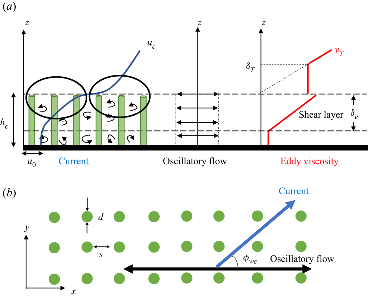
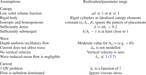
The field condition can be quite complicated due to the complexity of the canopy morphology, the detailed behaviour of shoaling waves and overlying current. Here, we choose to idealize the problem as a horizontal flow passing an array of cylinders, which allows us to focus on the drag-related effect. Some assumptions are imposed, which cover three aspects: canopy, wave and current. A sketch is provided in figure 1 to facilitate the following introductions. A summary of the assumptions is provided in table 1.

Figure 1.

Schematic sketch of wave–current flows in a dense submerged canopy. (a) Side view, (b) top view.

Table 1.

Summary of assumptions and parameter ranges of the proposed model.

2.1.1. Idealization of canopy

The canopy is simplified as an array of uniform rigid cylinders with a diameter, $d$, a canopy height, $h_c$, and a uniform spacing among canopy elements, $s$. Another important parameter of the canopy is the front area per unit volume, $a=d/s^{2}$. For a cylindrical canopy element, the solid volume fraction of the canopy, $\phi$, can be approximated as $\phi ={\rm \pi} ad/4$ (Nepf Reference Nepf2012). Strictly speaking, the arrangement of the cylinders, e.g. staggered or grid arrangement, may affect the hydrodynamic characteristics of the canopy, but here we neglect this influence and assume the canopy is an isotropic (any parameter of the canopy is not a function of flow direction) and homogeneous medium. This is acceptable under the assumption of low solid volume fraction, i.e. $\phi \ll 1$.

We would like to have a dense canopy, such that the KH vortices cannot fully penetrate the whole canopy. According to Ghisalberti (Reference Ghisalberti2009), the penetration depth of KH vortices for a submerged canopy is

(2.1)\begin{equation} \delta_p=\frac{0.23}{C_D a}, \end{equation}

where $C_D$ is a drag coefficient (close to 1). By requiring $\delta _p< h_c$, (2.1) gives that the solidity, $\hat {a}=ah_c$, must satisfy $\hat {a}>0.23/C_D$. Note that 0.23 is an empirical number obtained by fitting some measurements, so we expect the solidity to be over 0.2 to satisfy the requirement of a dense canopy. This can be achieved by having a tall canopy or a relatively high solid volume fraction.

Another assumption is that the canopy should be sufficiently submerged, e.g. the water depth should be at least comparable to (preferably much larger than) the canopy height. This assumption is required for treating wave-induced flow as a bottom-parallel oscillation. Also, it allows us to neglect the influence of surface processes on the in-canopy flow.

2.1.2. Idealization of wave

The wave-driven in-canopy flow, $u_w$, is approximated as an oscillatory flow with a sinusoidal temporal variation, i.e.

(2.2)\begin{equation} u_w= U_w\cos(\omega t), \end{equation}

where $t$ is time, $U_w$ is the amplitude and $\omega =2{\rm \pi} /T$ is the radian frequency of the oscillatory flow, with $T$ being the flow period. Many flume experiments (e.g. Lowe et al. Reference Lowe, Koseff and Monismith2005) showed that the oscillatory in-canopy flow can be fairly depth uniform. According to Ghisalberti & Schlosser (Reference Ghisalberti and Schlosser2013), a significant shear of the oscillatory velocity profile, which is due to the generation of a coherent vortex at the canopy top, only exists if the Keulegan–Carpenter number, $KC=U_wT/L_D$, is sufficiently large (they proposed $KC=5$ as an indicative threshold). Here, $L_D$ is a drag length scale defined as

(2.3)\begin{equation} L_D = \frac{1-\phi}{C_D a}, \end{equation}

where $C_D$ is the canopy drag coefficient (discussed in § 2.4). For typical aquatic canopies, $C_D \approx 1$ and $\phi \ll 1$, so $KC \approx 2{\rm \pi} (d/s)A_w/s$. Note that $d/s$ is much smaller than $1$ under the requirement of $\phi \ll 1$, so $KC$ can be comparable to or less than $5$ for $A_w/s$ less than $10$. This means that an oscillatory flow, for which the excursion amplitude does not far exceed the element spacing, can be approximated as a depth-uniform oscillatory flow inside the canopy. The previous flume experiments usually have $A_w/s$ comparable to or less than $1$. For typical coastal benthic canopies (e.g. coral reefs or seagrass meadows), for which $s$ is of $O$(1 cm), $A_w/s$ can still be less than $10$ under typical wave conditions, e.g. a wave of 50 cm height and 3 s period gives $A_w=12$ cm at a seabed that is 3 m below the mean sea level. We here restrict our model application to waves that give a moderate or small $A_w/s$, so a depth-invariant oscillatory flow can be assumed inside the canopy. With this limitation, the in-canopy oscillatory flow does not generate canopy-scale vorticity/turbulence, but still produces stem-wake turbulence. This is important for the parameterization of turbulent eddy viscosity in § 2.4. The model also neglects the vertical wave-induced orbital velocity, so the wave-induced mean Eulerian flow, for which an important driver is the wave stress at the top of the canopy, is omitted. Some discussions on this approximation will be presented in § 3.2. As previously mentioned, we only consider the wave's effect on the current, so the oscillatory in-canopy flow is assumed to be constant, and is taken as a model input.

2.1.3. Idealization of current

The current is taken as a horizontal flow at an angle to the axis of the oscillatory flow. The positive oscillatory flow direction is taken as the $x$-direction (see figure 1), so the current velocity, which is at an angle, $\phi _{wc}$, to the $x$-direction is defined as

(2.4)\begin{equation} \boldsymbol{u}_c = (u_{cx}, u_{cy})=u_c(\cos\phi_{wc}, \sin{\phi_{wc}}). \end{equation}

We assume the current is uniform in the $x-y$ plane, so the problem is reduced to a 1-DV problem, The combined flow velocity inside the canopy can therefore be written as

(2.5)\begin{equation} \boldsymbol{u}(z, t) = \left(U_w\cos(\omega t)+u_{cx}(z), u_{cy}(z)\right), \end{equation}

where $z$ is the vertical coordinate with $z=0$ being the bottom. The current is driven by a shear stress at the top of the canopy, $\boldsymbol {\tau }_{h}=(\tau _{hx}, \tau _{hy})$, and a gradient, $\boldsymbol {S}=(S_x, S_y)$. For a fully developed open-channel current with a water depth, $h$, the relative importance of $\boldsymbol {\tau }_h$ over $\boldsymbol {S}$ is represented by the ratio (Nepf Reference Nepf2012)

(2.6)\begin{equation} \frac{shear\ stress}{pressure\ gradient} \sim \frac{|\boldsymbol{\tau}_h|}{gh_c |\boldsymbol{S}|}=\frac{h}{h_c}-1, \end{equation}

where $g$ is the gravitational acceleration. For deeply submerged flow ($h/h_c \gg 1$), $\boldsymbol {\tau }_h$ is the dominant driving force, and $\boldsymbol {S}$ can be neglected. In such cases, $\boldsymbol {\tau }_h$ can also be taken as the current bottom shear stress experienced by the overlying flow. The in-canopy current is subject to a time-averaged Reynolds stress and canopy drag. In our model, the time-averaged Reynolds stress is given as the product of a turbulent eddy viscosity, $\nu _T$, and current velocity gradient, i.e.

(2.7)\begin{equation} \frac{\tau_i}{\rho}=\nu_T\frac{\partial u_{ci}}{\partial z}, \quad i=x,y. \end{equation}

Here, we ignore the viscous stress, since it is much weaker than the Reynolds stress in typical field conditions and also the laboratory conditions covered in this study. The instantaneous drag force is modelled using the conventional quadratic drag law adopted by many other researchers, so the time-averaged drag force, $\boldsymbol {f}_d$, is written as

(2.8)\begin{equation} \boldsymbol{f}_d=(f_{{d} x}, f_{{d} y})=\tfrac{1}{2}C_Da\overline{|\boldsymbol{u}(z,t)|\boldsymbol{u}(z,t)}, \end{equation}

where the overline denotes time averaging.

2.2. Governing equations

The governing equations for $u_{cx}$ and $u_{cy}$ inside the submerged canopy are

(2.9)\begin{equation} \left. \begin{aligned} & \displaystyle\frac{\partial}{\partial z}\left(\nu_T\frac{\partial u_{cx}}{\partial z}\right)={-}gS_x + f_{{ d} x},\\ \displaystyle & \frac{\partial}{\partial z}\left(\nu_T\frac{\partial u_{cy}}{\partial z}\right)={-}gS_y + f_{dy}. \end{aligned} \right\} \end{equation}

In this study, a current is prescribed by the canopy-top shear stress, $\boldsymbol {\tau }_h$ and the pressure gradient $\boldsymbol {S}$. With the closure models of $\nu _T$ and $(f_{dx}, f_{dy})$, (2.9) can be solved with two bottom boundary conditions.

Since we assume a dense canopy, the penetration depth of the canopy-scale shear layer is less than the canopy height, so there is a near-bed layer in which the in-canopy current is almost depth uniform. Therefore, a zero-gradient bottom boundary condition for current velocity is adopted

(2.10)\begin{equation} \frac{\partial u_{ci}}{\partial z}=0, \quad {\rm at}\ z=0, \ i=x,\,y. \end{equation}

This boundary condition also means that the bottom shear stress is ignored, and the model does not resolve the bottom boundary layer in the immediate vicinity of the bed. Therefore, the no-slip boundary condition is no longer applicable, and is replaced by a slip boundary condition

(2.11)\begin{equation} \boldsymbol{u}_c = \boldsymbol{u}_0=(u_{0x}, u_{0y})\quad {\rm at}\ z=0, \end{equation}

where $\boldsymbol {u}_0$ is the uniform in-canopy current velocity below the penetration depth. The value of $\boldsymbol {u}_0$ is iteratively determined by requiring that the obtained $u_{cx}$ and $u_{cy}$ profiles give the prescribed $\boldsymbol {\tau }_h$ at the canopy top, i.e.

(2.12)\begin{equation} \left.\nu_T\frac{\partial u_{ci}}{\partial z}\right|_{z=h_c} = \frac{\tau_{hi}}{\rho}, \quad i=x,y. \end{equation}

To better reveal the underlying physics and identify the dimensionless parameters controlling the in-canopy current, the governing equations are normalized. Here, we choose the shear velocity associated with $\boldsymbol {\tau }_h$ as the representative velocity

(2.13)\begin{equation} u_{*c} = \sqrt{\frac{|\boldsymbol{\tau}_h|}{\rho}}, \end{equation}

because $\boldsymbol {\tau }_h$ represents a key driving force for the in-canopy current, and it is also the resistance experienced by the flow above the submerged canopy. The flow velocity is normalized by $u_{*c}$

(2.14a–c)\begin{equation} \hat{\boldsymbol{u}}=\frac{\boldsymbol{u}}{u_{*c}}, \quad \hat{u}_w=\frac{U_w}{u_{*c}}, \quad \widehat{\boldsymbol{u}_c}=(\hat{u}_{cx},\hat{u}_{cy})=\left(\frac{u_{cx}}{u_{*c}}, \frac{u_{cy}}{u_{*c}}\right). \end{equation}

The vertical coordinate is normalized by the canopy height

(2.15)\begin{equation} \hat{z}=\frac{z}{h_c}. \end{equation}

The turbulence eddy viscosity is normalized by the product of $u_{*c}$ and $h_c$

(2.16)\begin{equation} \hat{\nu}_T =\frac{\nu_T}{u_{*c}h_c}. \end{equation}

The pressure gradients, $gS_x$ and $gS_y$, are normalized by $u_{*c}^{2}/h_c$

(2.17)\begin{equation} \hat{\boldsymbol{S}}=\left(\hat{S}_x, \hat{S}_y\right)=\left(\frac{gh_cS_x}{u_{*c}^{2}}, \frac{gh_cS_y}{u_{*c}^{2}}\right). \end{equation}

The canopy drag is normalized by $u_{*c}^{2}/h_c$

(2.18)\begin{equation} (\hat{f}_{dx}, \hat{f}_{dy})=\frac{(f_{dx}, f_{dy})}{u_{*c}^{2}/h_c} = \frac{1}{2}C_D\hat{a}\hat{u}_c^{2}(\beta_{cx}, \beta_{cy}), \end{equation}

where

(2.19)\begin{equation} \hat{a} = ah_c \end{equation}

is the solidity of the canopy, and $\beta _{cx}$ and $\beta _{cy}$ are defined as

(2.20)\begin{equation} (\beta_{cx}, \beta_{cy}) =\frac{\overline{|\hat{\boldsymbol{u}}(z,t)|\hat{\boldsymbol{u}}(z,t)}}{\hat{u}_c^{2}}. \end{equation}

Note that $\beta _c=\sqrt {\beta _{cx}^{2}+\beta _{cy}^{2}}=1$ for current-alone cases, so the value of $\beta _{ci}$ allows us to quantify the wave's effect on the mean drag experienced by the current, which will be discussed in § 2.4. The normalized governing equations are

(2.21)\begin{equation} \left. \begin{aligned} & \displaystyle \frac{\partial}{\partial \hat{z}}\left(\hat{\nu}_T\frac{\partial \hat{u}_{cx}}{\partial \hat{z}}\right)={-}\hat{S}_x + \hat{f}_{dx},\\ & \displaystyle \frac{\partial}{\partial \hat{z}}\left(\hat{\nu}_T\frac{\partial \hat{u}_{cy}}{\partial \hat{z}}\right)={-}\hat{S}_y + \hat{f}_{dy}. \end{aligned} \right\} \end{equation}

The normalized bottom boundary conditions are

(2.22)\begin{equation} \hat{\boldsymbol{u}}_c = (\hat{\boldsymbol{u}}_{0x}, \hat{\boldsymbol{u}}_{0y}) = \left(\frac{u_{0x}}{u_{*c}}, \frac{u_{0y}}{u_{*c}}\right), \quad {\rm at}\ \hat{z}=0, \end{equation}

and

(2.23)\begin{equation} \frac{\partial \hat{u}_{ci}}{\partial \hat{z}}=0, \quad {\rm at}\ \hat{z}=0, \ i=x,y. \end{equation}

The normalized solution must satisfy

(2.24)\begin{equation} \left(\hat{\nu}_T\frac{\partial \hat{u}_{cx}}{\partial \hat{z}},\quad \hat{\nu}_T\frac{\partial \hat{u}_{cy}}{\partial \hat{z}}\right) = (\cos\phi_{\tau h},\ \sin\phi_{\tau h}), \quad {\rm at}\ \hat{z}=1, \end{equation}

where $\phi _{\tau h}$ is the angle between $\boldsymbol {\tau }_h$ and the $x$-direction.

2.3. Turbulent eddy viscosity

For current in a dense submerged canopy, turbulence is generated around the top of the canopy due to a strong local vertical shear (hereafter referred to as shear turbulence) and in the stem wake (hereafter referred to as wake turbulence). The shear turbulence is at the canopy scale, while the wake turbulence is at the stem scale. We follow King et al. (Reference King, Tinoco and Cowen2012) to parameterize the turbulent eddy viscosity inside the canopy as the sum of two components corresponding to the two types of turbulence.

In the $k-\epsilon$ turbulence closure model of King et al. (Reference King, Tinoco and Cowen2012), the wake-turbulence-related eddy viscosity is given by

(2.25)\begin{equation} \nu_w = C_{\lambda}\frac{k_w^{2}}{\epsilon_w}, \end{equation}

where $C_{\lambda }$ is a constant, $k_w$ is the kinetic energy of wake turbulence and $\epsilon _w$ is the dissipation rate of wake turbulence. Following Tanino & Nepf (Reference Tanino and Nepf2008b), $\epsilon _w$ is given by

(2.26)\begin{equation} \epsilon_w = C_{\epsilon D}\frac{k_w^{3/2}}{d}, \end{equation}

where $C_{\epsilon D}$ is a constant. By substituting (2.26) into (2.25), we get

(2.27)\begin{equation} \nu_w=\frac{C_{\lambda}}{C_{\epsilon D}}\sqrt{k_w}d, \end{equation}

where Zhang et al. (Reference Zhang, Tang and Nepf2018) showed that $k_w$ in oscillatory flow can be modelled using the wake turbulent kinetic energy (TKE) model of Tanino & Nepf (Reference Tanino and Nepf2008b). For a small solid volume fraction, this model can be approximately written as

(2.28)\begin{equation} \sqrt{k_w} \approx \delta\left(\tfrac{1}{2}C_D ad\right)^{1/3}U_r, \end{equation}

where $\delta$ is a model constant and $U_r$ is a reference velocity. By substituting (2.28) into (2.27), we get

(2.29)\begin{equation} \nu_w =\left[\delta \frac{C_{\lambda}}{C_{\epsilon D}}\left(\frac{1}{2}C_D\right)^{1/3}\right](ad)^{1/3} U_r d=c_w (ad)^{1/3}U_r d. \end{equation}

King et al. (Reference King, Tinoco and Cowen2012), through model calibration, obtained $C_{\lambda }=0.01$ and $C_{\epsilon D}=0.2795$. Zhang et al. (Reference Zhang, Tang and Nepf2018), through fitting measurements, obtained that $\delta =0.76$, and they assumed $C_D=1.4$. Using these parameters, the value of $c_w$ is 0.024. We are aware that it is better to calibrate $c_w$ using existing experimental results, but we found that the model's performance (in terms of predicting the in-canopy current) weakly depends on the value of $c_w$. This is mainly because $\nu _w$ is only important in the very near-bed region, but the Reynolds stress in this region is negligible compared with the canopy drag and pressure gradient. Since another calibration parameter is introduced in the shear-related eddy viscosity (discussed later), we decided to simple accept the value $c_w=0.024$, so the model calibration process was simplified. We have conducted a sensitivity analysis for $c_w$, and found that the prediction changes by only a few per cent even if $c_w$ is doubled (taking $c_w=0.048$).

The representative velocity for wave–current flow is taken as the root-mean-square (r.m.s.) velocity near the bottom of the canopy, i.e.

(2.30)\begin{equation} U_r = \sqrt{\frac{1}{2}U_w^{2}+|\boldsymbol{u}_0|^{2}}. \end{equation}

Choosing the r.m.s. velocity is to include wake turbulence generated by both oscillatory and current flows. A conventional representative velocity of the oscillatory flow is its velocity amplitude, $U_w$. For the current, $|\boldsymbol {u}_0|$, which is the magnitude of the current velocity at the bottom of the canopy, is taken as the representative velocity. This is because the contribution of wake turbulence is most important in the lower part of the canopy, so using $|\boldsymbol {u}_0|$ means that $U_r$ represents the local flow. In the upper part of the canopy, the local current velocity is much stronger than $|\boldsymbol {u}_0|$, so the proposed $U_r$ is smaller than the local r.m.s. velocity. This should not lead to a big model error, because $\nu _w$ is much smaller than the shear-related eddy viscosity, $\nu _s$, in the upper part of the canopy.

The parameterization of $\nu _s$ is based on the flume experimental results of Ghisalberti & Nepf (Reference Ghisalberti and Nepf2004), who studied unidirectional flow in a submerged dense canopy. In their study, $\nu _s$ was estimated from measured shear and Reynolds stress. They found that $\nu _s$ increases from the bottom of shear layer, i.e. $z_1=h_c-\delta _e$, where $\delta _e$ is the depth of the region with a significant shear stress, to the top of the canopy. Above the canopy, $\nu _s$ first remains close to (or slightly larger than) that at the canopy top and subsequently decreases towards the free surface. This decrease is possibly due to the limited water depth in their flume experiments. They proposed the following scale for the maximum $\nu _s$:

(2.31)\begin{equation} \nu_{sm} \propto \Delta U \times t_{ml}, \end{equation}

where $t_{ml}$ is the thickness of the shear layer, which is defined from $z_1=h_c-\delta _e$ to a level in the free stream where the shear vanishes, and $\Delta U$ is the difference of current velocity between the two ends of the shear layer. They also showed that the Reynolds stress at the top of the canopy (see their figure 3) can be related to $\Delta U$ via

(2.32)\begin{equation} \frac{|\boldsymbol{\tau}_h|}{\rho}=u_{*c}^{2}=0.02\Delta U^{2}. \end{equation}

Thus, $\Delta U$ in (2.31) can be replaced by the current shear velocity, $u_{*c}$. Their measurements also showed that $t_{ml}$ is approximately 3 times $\delta _e$ (see their table 1), so $t_{ml}$ in (2.31) can be replaced by $\delta _e$. Thus, in this study, the maximum $\nu _s$ is

(2.33)\begin{equation} \nu_{sm} = c_s u_{*c}\delta_e, \end{equation}

where $c_s$ is a model parameter to be calibrated. In our model, $\delta _e$ is defined as the distance between the canopy top to a level where the mean shear stress is reduced to $5\,\%$ of $\boldsymbol {\tau }_h$. As will be shown later, the in-canopy current will be solved by iteration, so $\delta _e$ can be evaluated iteratively. Thus, no prior estimate of $\delta _e$ is required. Inside the canopy, we simply assume that $\nu _s$ linearly decreases from $\nu _{sm}$ at $z=h_c$ to $0$ at $z=0$. This simple vertical structure will capture the fact that the canopy-scale shear cannot fully penetrated the whole of the dense canopy. Although the vertical structure can be more complex, it can give satisfactory predictions, so we adopted it in our model.

Immediately above the canopy, it is assumed that the eddy viscosity is depth uniform and takes the value $\nu _T=\nu _{sm}$. At higher levels, the vertical structure of $\nu _T$ depends on the water depth above the canopy and the development of overlying flow. For modelling classic open-channel flow, a parabolic eddy viscosity profile is often applied, of which the near-bottom part can be approximated by a linear increase. Studying the eddy viscosity above the canopy would be an interesting research topic, but this is beyond the scope of this study. Here, for simplicity, our model assumes that the canopy is covered by a sufficiently large water depth, so the current velocity profile contains a logarithmic region above the canopy, for which the eddy viscosity linearly increases with the vertical coordinate: $\nu _T=\kappa u_{*c}(z-h_c)$, where $\kappa$ is the von Kármán constant. This linear eddy viscosity intersects with $\nu _T=\nu _{sm}$ at a transition level

(2.34)\begin{equation} \delta_T = \frac{c_s}{\kappa}\delta_e+h_c. \end{equation}

Note that the parameterization of the above-canopy $\nu _T$ does not affect the prediction of the in-canopy current if a current is specified by $\boldsymbol {\tau }_h$ at the top of the canopy and a pressure gradient.

Thus, the whole eddy viscosity profile can be written as

(2.35)\begin{equation} {\nu_T} = \left\{ \begin{array}{@{}ll} \nu_w+\dfrac{z}{h}\nu_{sm}, & 0 \le z < h_c,\\ \nu_{sm}, & h_c \le z \le \delta_T, \\ \kappa u_{*c}(z-h_c), & T. \end{array} \right. \end{equation}

An illustrative sketch of this profile is provided in figure 1. The normalized form of (2.35) is

(2.36)\begin{equation} {\hat{\nu}_T} = \left\{ \begin{array}{@{}ll} \hat{\nu}_w+\hat{\nu}_{sm}, & \hat{z} < 1,\\ \hat{\nu}_{sm}, & 1 \le \hat{z} \le 1+\dfrac{c_s}{\kappa}\hat{\delta}_e, \\ \kappa (\hat{z}-1), & \hat{z}>1+\dfrac{c_s}{\kappa}\hat{\delta}_e, \end{array} \right. \end{equation}

where

(2.37a–c)\begin{equation} \hat{\delta}_e=\frac{\delta_e}{h_c}, \quad \hat{\nu}_w=c_w\frac{(ad)^{4/3}}{\hat{a}}\sqrt{\frac{1}{2}\hat{u}_w^{2}+\hat{u}_0^{2}}, \quad \hat{\nu}_{sm} = c_s\hat{\delta}_e. \end{equation}

2.4. Drag force

Our model adopts a quadratic drag, i.e. (2.8), for the instantaneous drag force in a wave–current flow. Sarpkaya & Storm (Reference Sarpkaya and Storm1985) studied the in-line force on a cylinder in collinear wave–current flows. They found that the Morison equation with a quadratic drag force term can nicely fit the measured time series of the in-line force. Some researchers also adopted the same quadratic law in modelling time-varying in-canopy flows (Zeller et al. Reference Zeller, Zarama, Weitzman and Koseff2015; van Rooijen et al. Reference van Rooijen, Lowe, Rijnsdorp, Ghisalberti, Jacobsen and McCall2020) or analysing experimental results (Hu et al. Reference Hu, Suzuki, Zitman, Uittewaal and Stive2014). It should be noted that the nonlinearity of a quadratic law gives a considerable wave–current interaction on the time-averaged drag force, which has been pointed out by some researchers (van Rooijen et al. Reference van Rooijen, Lowe, Rijnsdorp, Ghisalberti, Jacobsen and McCall2020). In fact, the mean drag force can be significantly amplified by a co-existing oscillatory flow, i.e. the drag amplification factor, $\beta _c=\sqrt {\beta _{cx}^{2}+\beta _{cy}^{2}}$, is much larger than $1$ (see (2.20) for the definition of $\beta _{ci}$). In addition, if wave and current are at an angle of between $0^{\circ }$ and $90^{\circ }$, the mean drag force vector and the mean velocity vector may not be in the same direction.

To demonstrate the effect of oscillatory flows on mean drag, a simple illustration is provided here. We first define a wave–current ratio, which is the ratio of the amplitude of oscillatory velocity to the magnitude of current velocity

(2.38)\begin{equation} \alpha = \frac{U_w}{|\boldsymbol{u}_c|}=\frac{\hat{u}_w}{|\hat{\boldsymbol{u}}_c|}, \end{equation}

$\beta _{cx}$ and $\beta _{cy}$ can be given by

(2.39)\begin{equation} \left. \begin{aligned} \displaystyle & \beta_{cx}=\overline{\sqrt{\alpha^{2}\cos^{2}\omega t + 2\alpha\cos\omega t\cos\phi_{wc}+1}\times (\alpha\cos\omega t+\cos\phi_{wc})},\\ & \displaystyle \beta_{cy}=\overline{\sqrt{\alpha^{2}\cos^{2}\omega t + 2\alpha\cos\omega t\cos\phi_{wc}+1}\times \sin\phi_{wc}}. \end{aligned} \right\} \end{equation}

Equation (2.39) shows that both $\beta _c=\sqrt {\beta _{cx}^{2}+\beta _{cy}^{2}}$ and the angle between the drag force and the $x$-direction, $\phi _d=\tan ^{-1}(\beta _{cx}/\beta _{cy})$, are functions of $\alpha$ and $\phi _{wc}$. Here, we consider $\alpha$ between $0.1$ (an oscillatory flow much weaker than the current) and $10$ (an oscillatory flow much stronger than the current). We also choose four angles between wave and current, i.e. 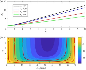$\phi _{wc}=0^{\circ }$, $30^{\circ }$, $60^{\circ }$ and $90^{\circ }$. Figure 2 presents the variation of $\beta _c$ and $\phi _d - \phi _{wc}$ with $\alpha$. For all wave–current angles, $\beta _c$ is very close to $1$ for small values of $\alpha$, showing that a weak oscillatory flow does not affect the mean drag force. For collinear wave–current flow ($\phi _{wc}=0^{\circ }$), $\beta _c$ increases dramatically as $\alpha$ becomes comparable to or larger than $1$, e.g. $\beta _c=1.49$ for $\alpha =1$, and $2.64$ for $\alpha =2$. This means a significant increase of mean drag force due to the co-existing oscillatory flow. It is also observed that a larger angle between the wave and current gives a smaller $\beta _c$. Note that $\phi _d-\phi _{wc}$ is zero for $\phi _{wc}=0^{\circ }$ (the flow is always collinear) and $\phi _{wc}=90^{\circ }$ (the oscillatory flow is symmetric). In figure 2(b), it can be seen that $\phi _d -\phi _{wc}$ is always negative (or $\phi _d$ is smaller than $\phi _{wc}$), so the mean drag vector veers towards the oscillatory flow. The magnitude of the veering increases with $\alpha$, and is up to approximately $20^{\circ }$ at $\alpha =10$ and $\phi _{wc}\approx 55^{\circ }$. For even larger values of $\alpha$ (e.g. $\alpha =100$), the veering is almost the same as for $\alpha =10$, so the largest veering angle is approximately $20^{\circ }$. This veering of drag vector will cause veering of the current velocity vector.

Figure 2.

Amplification factor and veering angle of the time-averaged drag force of wave–current in-canopy flows. (a) Amplification factor, $\beta _c$, (b) veering angle, $\phi _d - \phi _{wc}$ ($^{\circ }$).

Some researchers proposed that the instantaneous drag in wave–current flows can be given as the sum of a mean component and a time-varying component (e.g. Zhou & Graham Reference Zhou and Graham2000; Luhar et al. Reference Luhar, Coutu, Infantes, Fox and Nepf2010). If the drag coefficient of the mean (or current) component is insensitive to the co-existing oscillatory flow, such a decomposition means that the oscillatory flow has little effect on the mean drag experienced by the currents. As will be shown later, our choice of using the quadratic drag can indeed lead to accurate prediction of the current velocity profile, and capture a significant wave effect, so it is more suitable for modelling in-canopy drag.

The drag coefficient in (2.8) and (2.18) is estimated using the model proposed by Ghisalberti & Nepf (Reference Ghisalberti and Nepf2004)

(2.40)\begin{equation} {C_D(z)} = (1+10Re_d^{{-}2/3})\times \left\{ {\begin{array}{@{}ll} 1.4\left(\dfrac{z}{h_c}\right)^{2.5}+0.45, & 0 \le z/h_c < 0.76,\\ -4.8\left(\dfrac{z}{h_c}\right)+4.8, & 0.76 \le z/h_c \le 1, \end{array}} \right. \end{equation}

where $Re_d$ is a Reynolds number defined based on diameter $d$. This drag-coefficient model was derived by fitting measurements from unidirectional canopy flow experiments. It accounts for the vertical variation of $C_D$, which is because the free end of cantilevered cylinder disturbs the wake structure. To account for both the wave and current, $Re_d$ in our application is evaluated using the local r.m.s. velocity

(2.41)\begin{equation} Re_{d} = \frac{\sqrt{0.5U_w^{2}+|\boldsymbol{u}_c|^{2}}d}{\nu}, \end{equation}

where $\nu$ is the kinematic viscosity of water. The normalized form of (2.40) is

(2.42)\begin{equation} {C_D(\hat{z})} = \left(1+10\left(Re_*\sqrt{\frac{1}{2}\hat{u}_w^{2}+|\boldsymbol{u}_c|^{2}}\right)^{{-}2/3}\right)\times \left\{ {\begin{array}{@{}ll} 1.4\hat{z}^{2.5}+0.45, & 0 \le \hat{z} < 0.76,\\ -4.8\hat{z}+4.8, & 0.76 \le \hat{z} \le 1, \end{array}} \right. \end{equation}

where

(2.43)\begin{equation} Re_* = \frac{u_{*c}d}{\nu}. \end{equation}

2.5. Solution of current velocity profile

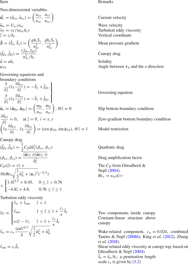
The normalized problem is formulated by a normalized governing equation, i.e. (2.21), two boundary conditions, that is (2.22) and (2.23), a closure model for the turbulent eddy viscosity, i.e. (2.36) and (2.37a–c), and a closure model for the canopy drag, i.e. (2.18), (2.38), (2.39) and (2.42). A summary of normalization and parameterization is provided in table 2. This system is controlled by the following six dimensionless parameters:

(2.44a–f)\begin{equation} Re_*,\quad \hat{u}_w, \quad \hat{S},\quad \hat{a}, \quad ad, \quad \phi_{\tau h}. \end{equation}

In dimensional form, the required input parameters are $(\boldsymbol {S}, U_w, \boldsymbol {\tau }_h)$ for prescribing the flow and $(a, h_c, d)$ for prescribing the canopy.

Table 2.

Summary of the proposed model, including normalization, governing equations, boundary conditions and parameterizations.

The normalized problem includes two parameters that must be iteratively determined, i.e. the bottom velocity, $(\hat {u}_{0x}, \hat {u}_{0y})$, and the penetration depth $\hat {\delta }_e$. With an initial guess of $(\hat {u}_{0x}, \hat {u}_{0y})$ and $\hat {\delta }_e$, the normalized system is solved numerically to give the normalized velocity profile. The numerical scheme is based on the finite volume method and is introduced in Appendix A. The solution is checked to see if it satisfies (2.24), i.e. if the mean shear stress at the canopy top meets the input. If not, $(\hat {u}_{0x}, \hat {u}_{0y})$ and $\hat {\delta }_e$ are updated, and a new iteration is conducted. This process continues until the solution converges.

The normalized governing equation of the current outside the canopy is

(2.45)\begin{equation} \frac{\partial}{\partial \hat{z}}\left(\hat{\nu}_T\frac{\partial \hat{u}_{ci}}{\partial \hat{z}}\right) ={-}\hat{S}_i. \end{equation}

Integrating this equation from the top of the canopy ($\hat {z}=1$) to $\hat {z}$ gives

(2.46)\begin{equation} \hat{\nu}_T\frac{\partial \hat{u}_{ci}}{\partial \hat{z}} ={-}\hat{S}_i(\hat{z}-1) + \hat{\tau}_{hi}, \quad i = x, y. \end{equation}

Using the profile of the normalized eddy viscosity, this equation can be integrated upward from $\hat {z}=1$, where the current velocity is obtained by numerically solving the in-canopy flow. The analytical solution of the above-canopy current is

(2.47)\begin{equation} {\hat{u}_{ci}} = \left\{ {\begin{array}{ll} \hat{u}_{hi}+\dfrac{\hat{\tau}_{hi}+\hat{S}_i}{c_s\hat{\delta}_e}(\hat{z}-1)-\dfrac{\hat{S}_i}{2c_s\hat{\delta}_e}(\hat{z}^{2}-1), & 1 < \hat{z} \le 1+\dfrac{c_s}{\kappa}\hat{\delta}_e,\\ \dfrac{\hat{\tau}_{hi}}{\kappa}\ln\left(\dfrac{\hat{z}-1}{\hat{z}_{0a,i}}\right)-\dfrac{\hat{S}_i}{\kappa}(\hat{z}-1), & \hat{z}>1+\dfrac{c_s}{\kappa}\hat{\delta}_e \end{array}}, \right. \end{equation}

where the apparent roughness is given by

(2.48)\begin{equation} \hat{z}_{0a,i}=\frac{c_s\hat{\delta}_e}{\kappa}\exp^{{-}1}\left(\frac{\kappa \hat{u}_{hi}}{\hat{\tau}_{hi}}+1+\frac{c_s\hat{\delta}_e}{2\kappa \hat{\tau}_{hi}}\hat{S}_i\right). \end{equation}

3.1. Model calibration

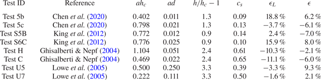
The parameter, $c_s$, in the shear-related eddy viscosity, i.e. (2.33), requires calibration. We chose the measurements from four groups of unidirectional flume experiments, which used an array of cylinders as the canopy, for the model calibration. Three dimensionless parameters, $\hat {a}$, $ad$, $h/h_c-1$, of the canopies in these tests are provided in table 3. The solidity $\hat {a}$ is from $0.22$ to $1.1$, so all canopies can be considered as dense canopies ($\hat {a} > 0.1$, cf. Nepf Reference Nepf2012). The parameter, $ad$, which represents the solid volume fraction, is from $0.01$ to $0.2$. The submergence, $h/h_c-1$, is between $0.9$ and $3.3$, which is applicable for typical submerged aquatic canopies.

Table 3.

Unidirectional flume tests used for model calibration.

Our model is driven by the mean shear stress at the canopy top and the mean pressure gradient of the open channel. These two parameters can only be estimated from the velocity measurements. In view of this, an iteration scheme is proposed to apply our model. The current is specified by a reference current velocity at a reference level slightly above the canopy, and there is reason for doing so. Note that the submergence of some tests is not very large (e.g. the water depth is only approximately twice of the canopy height). For these tests, our simple linearly increasing eddy viscosity above the canopy may not work. By having a reference velocity very close to the canopy top, the prediction of in-canopy flow will not be affected by the inadequacy of modelling above-canopy flow. The normalized mean pressure gradient is estimated following (2.6), i.e.

(3.1)\begin{equation} \hat{S}=\frac{h_c}{h-h_c}. \end{equation}

The value of the shear velocity, $u_{*c}$, is iteratively updated, until the model gives the reference current velocity. This iterative scheme was also applied to the wave–current tests in the next subsection.

The optimal value of $c_s$, which gives the best model–data agreement for the in-canopy current velocity, was obtained for each test in the calibration, and the results are provided in table 3. Here, the agreement is evaluated using the averaged r.m.s. error. It appears that the tests can be divided into two groups. The first group includes the first four rows of table 3, which have $c_s$ between $0.09$ and $0.14$. The second group includes the last four rows of table 3, which have $c_s$ between $0.39$ and $0.65$. By checking the values of $\hat {a}$, $ad$ and $h/h_c-1$, it seems that $c_s$ is correlated with the submergence $h/h_c-1$. In the first group, $h/h_c-1$ is close to $1$, so the thickness of water above the canopy is approximately the same as the canopy height. In the second group, $h/h_c-1$ is between $2.4$ and $3.3$, meaning that the thickness of water above the canopy is approximately $2.4$ to $3.3$ times the canopy height.

The shear-related eddy viscosity characterizes the mixing of momentum due to the canopy-scale KH vortex in the upper part of the canopy. In fact, the characteristics of the KH vortices are controlled by the submergence of the canopy. For instance, Ghisalberti & Nepf (Reference Ghisalberti and Nepf2002) showed that the translation velocity of KH vortices increases with the submergence of the canopy. Thus, it can be argued that the shear-related eddy viscosity is also affected by the submergence. The size of the KH vortex is comparable to $h_c$, so it is possible that the limited water depth above the canopy affects the development or the behaviour of KH vortices, if $h/h_c-1$ is close to or smaller than 1. Accurately quantifying $c_s$ as a function of $h/h_c-1$ requires a large set of experiments, especially for the tests with $h/h_c-1$ between $1.3$ and $2.4$. Since the focus of this study is on wave–current interaction within the canopy, we shall leave this for the future. Here, we simply adopt a three-leg structure that gives an increasing $c_s$ between $(h/h_c-1)=1.3$ and 2.4

(3.2)\begin{equation} {c_s} = \left\{ \begin{array}{@{}ll} 0.12, & h/h_c-1 < 1.3,\\ 0.3818(h/h_c-1)-0.3764, & 1.3\le h/h_c-1 < 2.4,\\ 0.54, & h/h_c-1 \geq 2.4. \end{array} \right. \end{equation}

For very low submergence, large-scale flow structure (here the KH vortex) will lead to undulation of the free surface, or the propagating wave's trough may touch the canopy. In such cases, the free surface dynamics may also control the vertical momentum transfer in the upper canopy. We leave the investigation of very low submergence to the future.

Figure 3 presents the model–data comparisons for the eight tests in the calibration. To quantify the error, we introduced an error index

(3.3)\begin{equation} \epsilon = \frac{\sum prediction-\sum measurement}{\sum measurement}. \end{equation}

This index measures the relative error in predicting the overall flow rate. Two error values were evaluated. The first one, $\epsilon$, was calculated using all measured data points below the canopy top ($0\le \hat {z}<1$), so it indicates the overall model performance for in-canopy current. The second one, $\epsilon _L$, was calculated using the data points below the penetration depth ($0\le \hat {z}<1-\hat {\delta }_e$), so it shows the model error for the lower part of the canopy. The results are presented in the last two columns of table 3.

Figure 3.

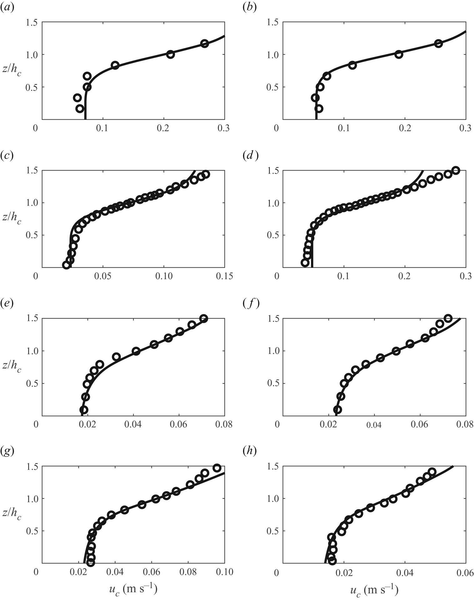
Prediction of in-canopy current profile for pure-current flume tests (circles, measurements; solid lines, predictions; see table 3 for test conditions). (a) Test 5b, $c_s = 0.12$. (b) Test 5c, $c_s = 0.12$. (c) Test S5B, $c_s = 0.12$. (d) Test S6C, $c_s = 0.12$. (e) Test U5, $c_s = 0.54$. ( f) Test U7, $c_s = 0.54$. (g) Test H, $c_s = 0.54$. (h) Test C, $c_s = 0.54$.

The model captures the vertical variation of current inside the canopy ($0\le \hat {z}<1$). A nearly depth-invariant current is predicted in the lower part of the canopy for the four shallow-submergence tests with $c_s=0.12$. For the four deep-submergence tests with $c_s=0.54$, the shear (vertical gradient of current velocity) is visible in the lower part of the canopy, but the magnitude is much lower than that near the top of the canopy. The shape of the profile, which is characterized by an infection point around the top of the canopy ($\hat {z}=1$), is well produced by the model. There are some discrepancies in the above-canopy region, indicating that the proposed eddy viscosity above the canopy can be further refined for describing the shear layer above the canopy. The error, $\epsilon _L$, of the lower layer is generally around 10 %, while the error, $\epsilon$, of the whole canopy is below 10 %.

3.2. Model validation

In this section, the model is applied to predict the in-canopy current for wave–current flows through a submerged dense canopy. The recent flume study by Chen et al. (Reference Chen, Lou, Liu, Ma, Liu, Zhong and Zhang2020) are used for model validation. In this study, co-directional wave–current flows were generated in a 50 m long, 1.2 m wide and 0.8 m deep flume. A 6 m long vegetated zone was installed in the middle of the flume. The submerged canopy was an array of unstaggered cylinders ($d=8\,$mm). We choose the two canopy configurations (b,c), which have uniform vegetation density throughout the entire canopy, for our model validation. The canopy height was 0 cm, while the water depth was 0.7 m. For each canopy configuration, there were four wave–current tests (named as Test 6 to Test 9). In these tests, the waves have the same period (1.8 s) and wave heights increased from 6 cm (Test 6) to 12 cm (Test 9). The current was specified by the total flow rate in the flume, and the ‘same’ current of a $140$ s^-1 flow rate was produced in all tests, which means the cross-section-averaged current velocity was approximately $17\,\textrm {cm}\,\textrm {s}^{-1}$. The flow velocity was sampled at a 5 cm vertical interval using an acoustic Doppler velocimetry (ADV) installed in the void among the cylinders. The ADV measurements showed that the oscillatory flow inside the canopy was approximately $10\sim 20\,\textrm {cm}\,\textrm {s}^{-1}$, and was quite depth uniform. The in-canopy current had the typical vertical profile of the in-canopy unidirectional flow, and the current magnitude was generally below $10\,\textrm {cm}\,\textrm {s}^{-1}$ (see their figure 5).

The input parameters are determined as follows. The amplitude of the oscillatory flow measured at 10 cm from the bottom (or 20 cm below the canopy top) was taken as the amplitude of the in-canopy oscillatory flow, $U_w$. The current is specified by a reference current velocity, $u_{cr}$, measured at $5\,\textrm {cm}$ above the canopy (or $35\,\textrm {cm}$ from the bottom). The canopy is described by $d=8\,\textrm {mm}$, $h_c=30\,\textrm {cm}$, $h=70\,\textrm {cm}$ and the front area per unit volume, $\alpha$. Table 4 summarizes the values of $U_w$, $u_{cr}$ and $\alpha$, for all tests involved in the model validation.

Table 4.

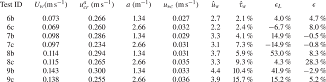
Input parameters and key output parameters of the wave–current tests of Chen et al. (Reference Chen, Lou, Liu, Ma, Liu, Zhong and Zhang2020).

${}^{a}$The reference level is $z=35\,\textrm {cm}$.

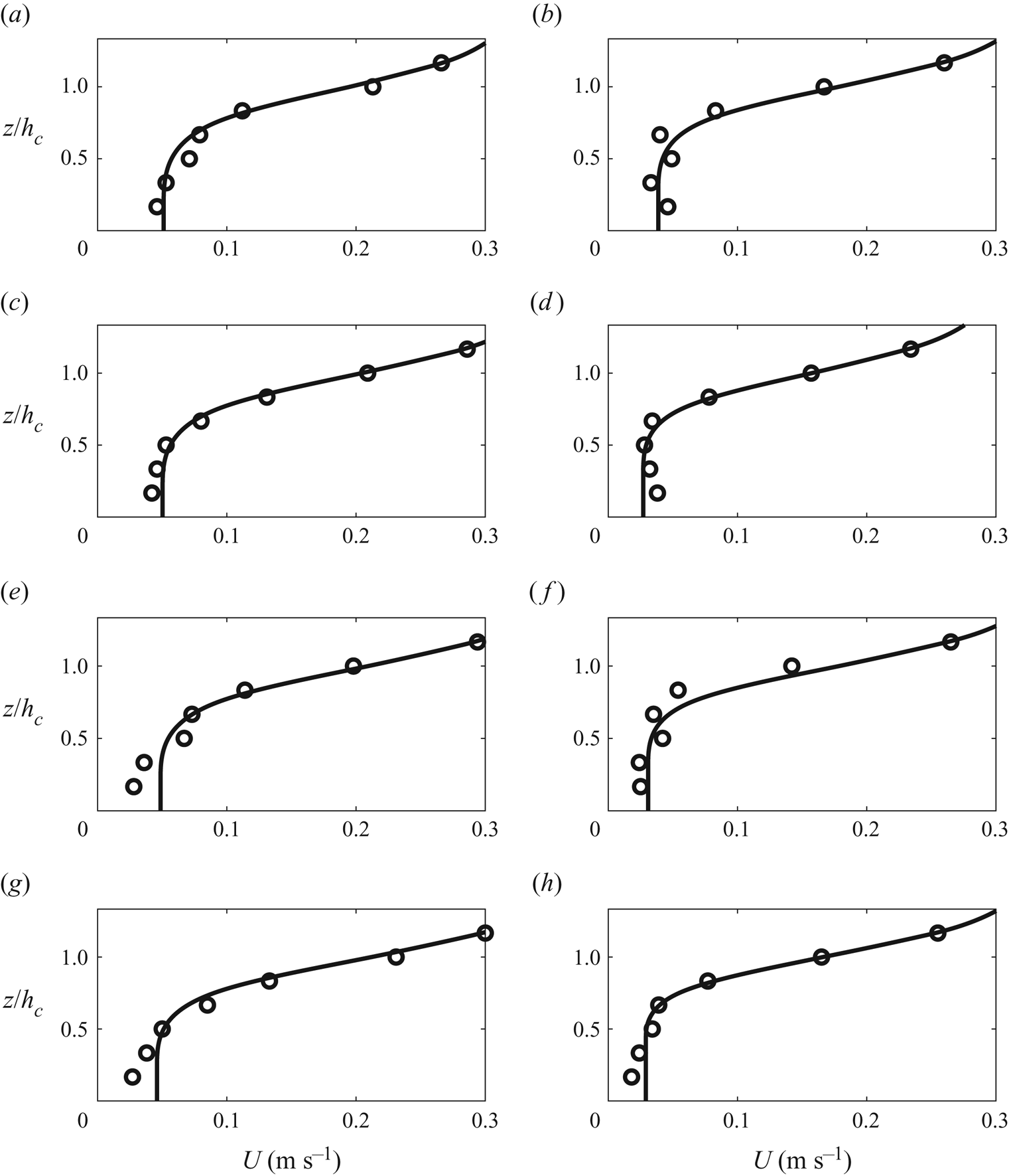
The comparisons between measurements and predictions are shown in figure 4, and the quantification of model error is provided in the last two columns of table 4. Overall, the model–data agreement is similar to the pure-current cases in figure 3. The current profile in the upper part of the canopy, where a strong vertical gradient is present, is well predicted by the model. This suggests that the simple eddy viscosity model, which is calibrated using only pure-current flows, works for these wave–current flume tests. Using the predicted shear velocity, $u_{*c}$, it is found that the normalized wave velocity, $\hat {u}_w=U_w/u_{*c}$ is generally between 2 and 4. Thus, it can be speculated that an in-canopy oscillatory flow with $\hat {u}_w<4$ has insignificant effect on the current-generated KH vortices at the canopy top. The model also predicts a weak in-canopy flow with little vertical gradient in the lower part of the canopy. For c-group tests (denser canopy, the right column of figure 4), both the prediction and the measurement have a quite depth-uniform flow near the bottom of the canopy. For some b-group tests (sparser canopy, see Tests 8b and 9b), the measured velocity profile seems to have some vertical gradient near the bottom. Using (2.1) and simply $C_D=1$, the penetration depth for b-group tests ($a=1.34\,\textrm {m}^{-1}$) is found to be $17\,\textrm {cm}$, which is approximately half of the canopy height. Thus, the canopy should be sufficiently dense to give a lower in-canopy layer, where the drag force is mostly balanced by the pressure gradient. As shown in figure 5(a), the unidirectional flow test (Test 5b) of the same canopy indeed has a quite depth-uniform lower layer in the current profile. One possible explanation of the observed near-bottom velocity gradient is the spatial variation of drag coefficient. A uniform in-canopy flow requires a constant drag coefficient and a balance between mean drag and pressure gradient. In wave–current flows, the mean drag is influenced by the drag amplification factor, $\beta _c$, defined in (2.20). Note that $\beta _c$ is partly influenced by the amplitude of oscillatory flow. In the very vicinity of the bottom, the oscillatory flow should have some vertical variation, since it must be reduced to zero at the bottom to meet the no-slip boundary condition. This will lead to a strong vertical variation of $\beta _c$, which cannot be captured by our model, due to the assumption of a depth-uniform oscillatory flow. The error, $\epsilon _L$, of the lower layer indeed increases with the wave condition (wave amplitude increases from Test 6b to 9b), but except for Tests 8b and 9b, $\epsilon _L$ is approximately 10 %, which is comparable to that of the calibration tests. The overall error of the whole layer, except for one test (Test 8c), is also below 10 %. Thus, the model performance for the validation tests is similar to that for the calibration tests.

Figure 4.

Model validation for current velocity profiles in wave–current canopy flows (circles, measurements; solid lines, predictions). (a) Test 6b. (b) Test 6c. (c) Test 7b. (d) Test 7c. (e) Test 8b. ( f) Test 8c. (g) Test 9b. (h) Test 9c.

Figure 5.

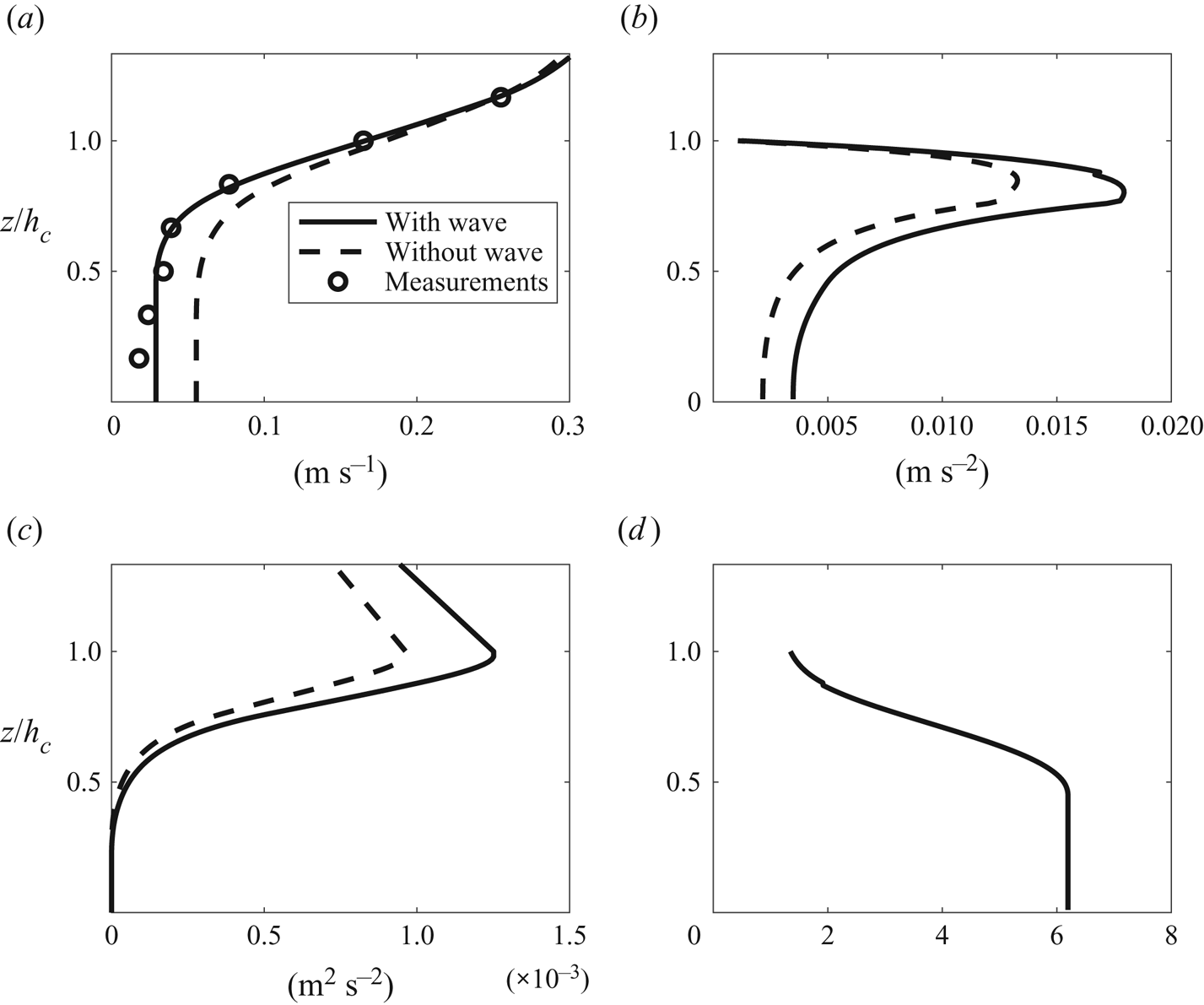
Prediction of Test 9c (the top of the canopy is at $z=0.3$ m): (a) current velocity $u_c$, (b) drag force $f_d$, (c) Reynolds shear stress $\tau /\rho$, (d) drag amplification factor $\beta _c$.

To show more details of our model, here the predictions of the mean canopy drag, Reynolds stress and drag amplification factor of a representative test, Test 9c, are presented in figure 5. To highlight the effect of waves, a corresponding pure-current prediction was conducted by setting the oscillatory velocity to zero. The results are also provided in figure 5 for comparison. From figure 5(a), it can be seen that adding an oscillatory flow significantly reduces the in-canopy current velocity by roughly a factor of 2. The driving force of the current, i.e. the pressure gradient and the shear stress at the canopy top (see figure 5c), in the wave–current prediction is only approximately $30\,\%$ larger than that in the pure-current prediction. Accordingly, the mean canopy drag of the wave–current prediction is approximately $30\,\%$ to $50\,\%$ larger than that of the pure-current prediction (see figure 5b). The drag amplification factor, $\beta _c$, of the wave–current prediction, however, is up to 6.5 inside the canopy (see figure 5d), since the ratio of wave velocity to current velocity is approximately 5 inside the canopy. Thus, the current velocity of the wave–current prediction must be $50\,\%$ smaller than that of the pure-current prediction, in order to give the required mean drag. This comparison demonstrates that the nonlinear wave–current interaction originating from the quadratic drag law indeed can have a pronounced effect on in-canopy current. More in-depth discussions will be provided in the next section.

The potential contribution of wave-induced mean canopy flow to wave–current interaction is worth some discussion. According to Luhar et al. (Reference Luhar, Coutu, Infantes, Fox and Nepf2010), waves pump momentum and energy into a submerged canopy, which leads to an in-canopy mean flow. Assuming that the energy dissipation due to canopy drag balances the wave-induced energy influx, the wave-induced momentum influx or a mean wave stress at the top of the canopy can be written as

(3.4)\begin{equation} \frac{\tau_w}{\rho}=(-\overline{uw})_{w, top} = \dot{E}/c, \end{equation}

where $\dot {E}$ is the energy dissipation rate within the canopy, and $c$ is the wave celerity. Assume depth-uniform oscillatory flow and a quadratic drag law

(3.5)\begin{equation} \dot{E} = \int_0^{h_c} U_w F_D\,{\rm d}z = \frac{2}{3{\rm \pi}}\rho C_Dah_cU_w^{3}. \end{equation}

Substitute (3.5) into (3.4), the wave stress at canopy top is

(3.6)\begin{equation} \frac{\tau_w}{\rho}=\frac{2}{3{\rm \pi}}\rho a C_D \left(\frac{U_w}{c}\right)U_w^{2}h_c. \end{equation}

The relative importance of the wave-induced mean in-canopy flow can be assessed by the ratio of $\tau _w$ to $\tau _h$, i.e.

(3.7)\begin{equation} \hat{\tau}_w = \frac{\tau_w}{\tau_h}=\frac{2}{3{\rm \pi}}\hat{a}C_D\left(\frac{U_w}{c}\right)\hat{u}_w^{2}. \end{equation}

Based on (3.7), the contribution of wave-induced mean flow increases with the solidity of the canopy ($\hat {a}$), the relative strength of the wave ($\hat {u}_w$), but decreases with wave celerity. Using wave celerity estimated by linear wave theory, $\hat {\tau }_w$ of the eight validation tests is evaluated and presented in the last column of table 4. The highest $\hat {\tau }_w$ ($15.7\,\%$) is from Test 9c, since this test has the highest value of $U_w/c$, and the larger $\hat {a}$. For most of the tests, $\hat {\tau }_w$ is less than $10\,\%$, so the mean wave stress is much smaller than the mean shear stress at the canopy top. Therefore, it is reasonable to neglect wave-induced mean canopy flow in these tests. In shallow coastal regions, the ratio $U_w/c$ is usually around or less than 0.1 (e.g. 1 m high wave with a $4\ {\rm s}$ wave period gives $U_w/c=0.14$ for a water depth of $3\ {\rm m}$). Assuming $C_D$ is around $1\sim 2$, a wave-induced mean flow is not important if $2\hat {a}\hat {u}_w^{2}/3{\rm \pi}$ is of $O(1)$.

4.1. Collinear wave–current flow

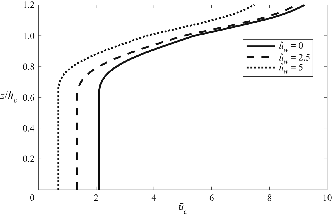
An oscillatory flow inside the canopy amplifies the mean canopy drag force experienced by the current. Under the same driving force, the in-canopy current of a wave–current flow can be significantly reduced from that of a unidirectional flow. This effect can be illustrated by comparing a series of collinear wave–current predictions with varying values of $\hat {u}_w$. Figure 6 compares three predictions with the same submergence ($S=1$), canopy density ($\hat {a}=1$) but different wave strengths ($\hat {u}_w=0$, 2.5 and 5). It can be clearly seen that the current velocity reduces significantly with increasing $\hat {u}_w$, In the near-bottom region, the current under $\hat {u}_w=5$ is less than half of that without a wave ($\hat {u}_w=0$). The reduction reduces towards the top of the canopy, i.e. at $z/h_c=1$ the current under $\hat {u}_w=5$ is only approximately $17\,\%$ smaller than that without a wave. Therefore, it can be concluded that the wave's effect is more important in the lower part of the canopy.

Figure 6.

Normalized current velocity profile for a shallow-submergence canopy ($\hat {S}=1$, $ad=0.02$, $\hat {a}=1$, $Re_{*}=500$).

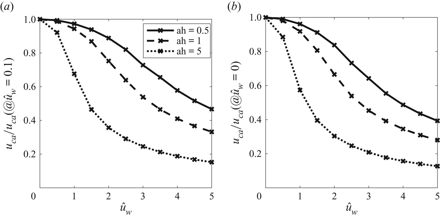
To give an overall picture of wave-related reduction of in-canopy current velocity, the depth-averaged in-canopy current velocity, $\hat {u}_{ca}$, is considered. For given values of $Re_*$, $ad$, $\hat {a}$ and $\hat {S}$, $\hat {u}_{ca}$ is a function of $\hat {u}_w$. We calculated $\hat {u}_{ca}$ for $\hat {u}_w$ between 0 and 5, and evaluated the ratio $r_u=\hat {u}_{ca}/\hat {u}_{ca,0}$, where $\hat {u}_{ca,0}$ is from the pure-current prediction. Here, $r_u$ quantifies the overall reduction of in-canopy current. The results for the two submergence (shallow, $\hat {S}=1$, and deep $\hat {S}=1/3$) and three canopy solidities ($\hat {a}=0.5, 1, 5$) are presented in figure 7. It can be easily seen that more reduction of current occurs for a denser canopy and stronger wave condition, while the effect of submergence is insignificant. For a sparse canopy ($\hat {a}=0.5$), the reduction is approximately $10\,\%$ ($r_u=0.9$) under $\hat {u}_w\approx 2$, and is increased to approximately $50\,\%$ under $\hat {u}_w\approx 5$. For a dense canopy ($\hat {a}=5$), a $10\,\%$ reduction can be achieved for $\hat {u}_w<1$, and $\hat {u}_w=5$ can give $80\sim 90\,\%$ reduction of $\hat {u}_{ca}$. Under the same driving force, a denser canopy has a smaller in-canopy current, which gives a larger wave–current ratio, $\alpha =U_w/u_c$. The drag amplification factor increases with $\alpha$, so a dense canopy has more reduction of the in-canopy current velocity in order to maintain a drag force similar to that in a sparse canopy.

Figure 7.

The variation of depth-averaged in-canopy flow with the relative wave strength $\hat {u}_w$: (a) shallow submergence, average in-canopy velocity, $\hat {S}=1, c_s=0.12$; (b) deep submergence, average in-canopy velocity, $\hat {S}=1/3, c_s=0.54$.

4.2. Wave and current at an angle

As shown in figure 2, when the wave and current inside the canopy are at an angle between $0\,^{\circ }$ and $90\,^{\circ }$, the drag force vector is not aligned with the current velocity vector, but veers towards the waves. For a fully developed in-canopy current, if the two driving forces of in-canopy current, i.e. the mean shear stress at the canopy top and the mean pressure gradient, are in the same direction, the total drag force (vertical integral of canopy drag) must balance the sum of the two driving forces. Therefore, for pure-current flow, the current velocity vector must be aligned with the driving force vectors. For wave–current flows, however, the current velocity vector should veer away from the driving force vectors (here ‘away’ means enlarging the angle between the current velocity vector and the axis of the oscillatory flow) to offset the toward-wave veering of the mean drag force. This phenomenon is discussed in this section.

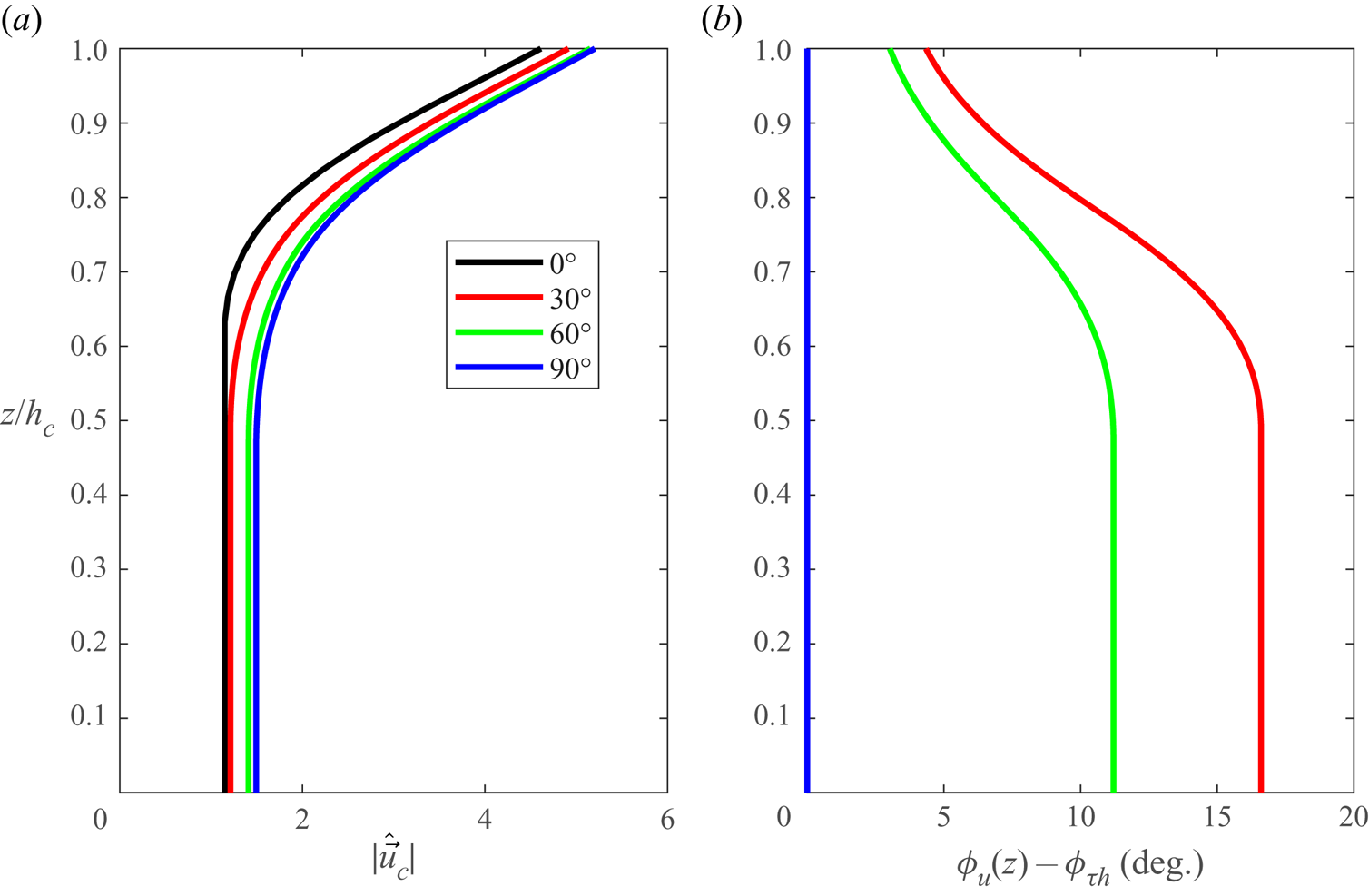
We shall begin with presenting some typical predictions of current velocity profiles. Here, we consider four predictions with different wave–current angles ($\phi _{\tau h}=0^{\circ }$, $30^{\circ }$, $60^{\circ }$ and $90^{\circ }$), which share the same non-dimensional parameter set ($Re_*=500$, $ad=0.02$, $\hat {a}=1$, $\hat {u}_w=3$ and $\hat {S}=1$). The veering of the current is given by the angle between the current velocity and the driving force, i.e. $\Delta \phi =\phi _{wc}-\phi _{\tau h}$, where $\phi _{wc}$ is the direction of current velocity. The oscillatory velocity is along the axis of $\phi _{wc}=0$, and $\phi _{\tau h}$ is between 0 and $90^{\circ }$, so a positive $\Delta \phi$ means the velocity vector veers away from the axis of the oscillatory flow. As shown in figure 8(a), the reduction of current velocity magnitude decreases with $\phi _{\tau h}$, this is because a larger $\phi _{wc}$ (due to a larger $\phi _{\tau h}$) gives a smaller drag amplification factor and hence allows a larger current velocity. The value of $\Delta \phi$ is 0 for collinear ($\phi _{\tau h}$) and perpendicular ($\phi _{\tau h}$) wave–current flows in our model. For $\phi _{\tau h}=30^{\circ }$ and $60^{\circ }$, $\Delta \phi$ increases from less than $5^{\circ }$ at the canopy top to approximately $11^{\circ }$ and $17\,^{\circ }$ at the bottom, respectively. In the lower part of the canopy ($\hat {z}<0.5$), where shear stress is negligible and the current velocity is almost uniform, the mean drag force balances the mean pressure gradient, so a uniform away-from-wave veering of current velocity vector is established to offset the towards-wave veering of drag. For instance, the $\Delta \phi =11^{\circ }$ in the $\phi _{\tau h}=60^{\circ }$ case gives a $\phi _{wc}=71^{\circ }$ in the lower part of the canopy. The wave–current ratio $\alpha =U_w/|\boldsymbol {u}_c|$ is approximately 2 locally, so the towards-wave veering of the mean drag is approximately $-10^{\circ }$ (see figure 2), which just offsets the $\Delta \phi$.

Figure 8.

Vertical profiles of current velocity magnitude and veering of current direction for different wave–current angles. In all predictions: $Re_*=500$, $ad=0.02$, $\hat {a}=1$, $\hat {u}_w=3$ and $\hat {S}=1$. (a) Current velocity. (b) Veering of current direction.

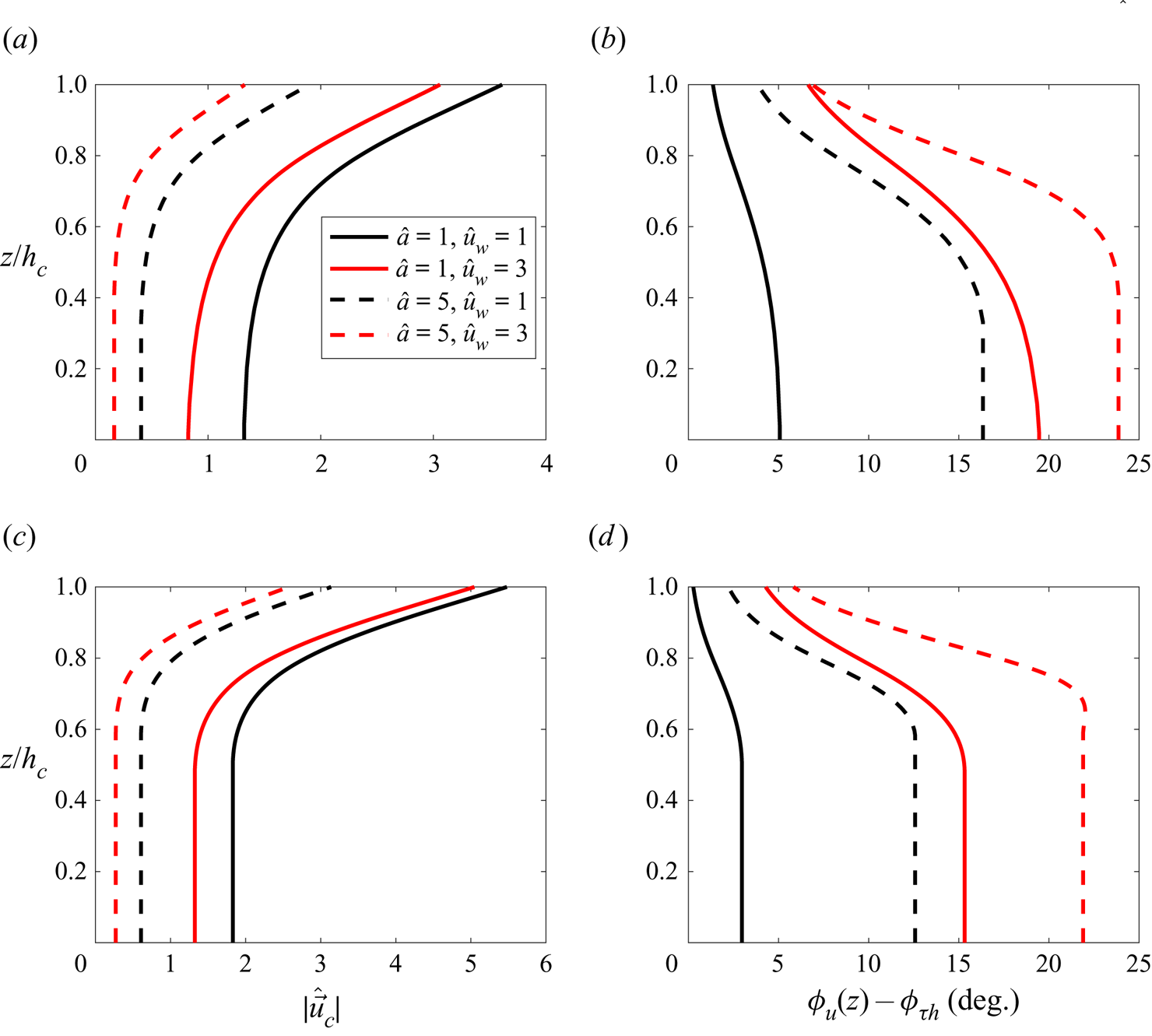
To illustrate the effects of the canopy density, relative wave strength and submergence, here, we compare the predictions of $\phi _{\tau h}=45^{\circ }$ wave–current flows with $Re_*=500$, $ad=200$. We tested $\hat {a}=[1,5]$ and $\hat {S}=[1, 1/3]$, so a total of eight predictions are provided in figure 9. The following two remarks can be made.

1. (i) Increasing relative wave strength increases the veering of current (the comparison between red and black lines in figure 9b,d).

2. (ii) Increasing the canopy solidity increases the veering of current (the comparisons between the dashed and solid lines in figure 9b,d).

These two remarks can be interpreted by considering the wave–current ratio, $\alpha$. A larger relative wave strength directly increases $\alpha$. A denser canopy will lead to weaker in-canopy current, $\hat {\boldsymbol {u}}_c$ under a prescribed driving force, since the penetration of overlying flow into the canopy is hindered. Thus, under the same wave velocity $\hat {u}_w$, the ratio $\alpha =|\hat {u}_w/\hat {\boldsymbol {u}}_c|$ is increased. As shown in figure 2, the veering angle increases with $\alpha$, so the two remarks are explained.

Figure 9.

The effect of the canopy density, relative wave strength and submergence on wave–current canopy flows ((a,c) profiles of current velocity magnitude, (b,d) profiles of current veering). (a) Current velocity, deep submergence $\hat {S}= 1/3$. (b) Veering of current direction, deep shallow submergence $\hat {S}= 1/3$. (c) Current velocity, shallow submergence $\hat {S}= 1$. (d) Veering of current direction, shallow submergence $\hat {S} = 1$.

The effect of submergence (the comparison between figure 9b,d) appears to be less significant. Reducing $\hat {S}$ leads to a weaker $|\hat {\boldsymbol {u}}_c|$ (compare figure 9a,c). This is because $\hat {S}$ is balanced by canopy drag in the near-bed region, so $\hat {S}$ is proportional to $|\hat {\boldsymbol {u}}_c|^{2}$. Reducing $\hat {S}$ from 1 to 1/3 would reduce $|\hat {\boldsymbol {u}}_c|$ by a factor of 0.58. This is not a huge reduction, so $\alpha$ and hence the veering angle is not changed a lot. If we were to compare very deep submergence ($\hat {S}\to 0$) with very shallow submergence ($\hat {S}\to \infty$), the difference could become much bigger.

The veering angle of the mean drag vector becomes independent of $\alpha$ for $\alpha >10$, i.e. the contours in figure 2(b) becomes almost vertical at $\alpha =10$, and the largest veering angle is slightly above $20^{\circ }$ for $\phi _{wc}$ around $55^{\circ }$. Thus, it can be expected that the veering of in-canopy current has an upper limit around $20^{\circ }$. For instance, the cases with $\hat {a}=5$ (dense canopy) and $\hat {u}_w=3$ (strong wave) in figure 9 (the red dashed lines) have $\Delta \phi$ slightly over $20^{\circ }$.