How do collisionless shocks generate the dissipation necessary to satisfy mass, momentum and energy continuity? For perpendicular shocks, ion reflection and gyration back to the layer are responsible for dissipation beyond resistive or anomalous heating (Forslund et al. Reference Forslund, Quest, Brackbill and Lee1984; Kennel, Edmiston & Hada Reference Kennel, Edmiston and Hada2013). In contrast, for quasi-parallel shocks, reflected or shock-heated ions can escape upstream without gyrating back to the layer (Edmiston, Kennel & Eichler Reference Edmiston, Kennel and Eichler1982). One possible dissipation mechanism posits that these counter-streaming ions steepen foreshock whistler waves until the waves are able to reflect upstream particles, effectively advancing the shock front forward (Burgess Reference Burgess1989; Pantellini et al. Reference Pantellini, Heron, Adam and Mangeney1992; Scholer Reference Scholer1993; Chen et al. Reference Chen2021). These steepened pulses merge into a dynamic, non-stationary and extended transition layer, behind which the magnetohydrodynamic continuity equations are ultimately satisfied (Schwartz & Burgess Reference Schwartz and Burgess1991; Scholer, Kucharek & Shinohara Reference Scholer, Kucharek and Shinohara2003; Lucek et al. Reference Lucek, Horbury, Dandouras and Rème2008). This inherent non-stationarity of parallel shocks makes in situ observations difficult and motivates the development of reproducible laboratory platforms.

Figure 1.

(a) Cartoon diagram of the experimental set-up during a shot. Guns at the north pole (6) produce the background plasma, which fills the field lines (black) produced with a Helmholtz coil pair (not shown) and a single mirror coil (5). The high- $\beta$ piston (2) enters the vessel from the coaxial plasma gun barrel (1) and expands radially as it translates. The four hanging double probes (3) are shown at fixed locations of R = +0.15 and Z = –0.86, –0.25, +0.52, +0.88 m. The multi-tip Langmuir probe (4) can scan the shaded area. (b) The five plots show the initial radial profiles for the primary scan at 3.0 mT field. The coloured-region error bars represent systematic uncertainty, and shot-to-shot fluctuations are smaller.

Figure 1. Long description

Panel A: A cartoon diagram illustrates the experimental setup. The diagram shows a vessel with various components labeled. Guns at the north pole produce background plasma, which fills the field lines generated by a Helmholtz coil pair and a single mirror coil. A high-piston enters the vessel from a coaxial plasma gun barrel and expands radially as it translates. Four hanging double probes are positioned at fixed locations, and a multi-tip Langmuir probe can scan a shaded area. Panel B: Five plots display the initial radial profiles for the primary scan at a 3.0 millitesla field. Each plot shows different parameters: electron density, electron temperature, magnetic field component Bz, plasma beta, and ion velocities. The x-axis for all plots represents the radial distance in meters, ranging from 0 to 0.5 meters. The y-axes represent different units for each parameter: electron density in units of 10^18 per cubic meter, electron temperature in electron volts, magnetic field component Bz in millitesla, plasma beta, and ion velocities in centimeters per microsecond. The plots include colored-region error bars representing systematic uncertainty, with shot-to-shot fluctuations being smaller. The data points show trends and variations in the initial radial profiles.

The substantial challenges to producing properly collisionless parallel shocks in the laboratory means that suitable platforms are scarce. Older pulsed power experiments, which used magnetic pistons with poor shot-to-shot variability, were solidly in the collisional regime (Craig & Paul Reference Craig and Paul1973). Recently, laser platforms have had success in launching collisionless shocks (Fiuza et al. Reference Fiuza2020), but at parameters where the background magnetic field is dynamically unimportant (i.e. $\beta \equiv P_{\textrm {plasma}}/P_{\textrm {mag.}} \gg 1$ ). Other laser plasma experiments have observed beam instabilities important to quasi-parallel collisionless shocks, but have not observed compression or shock heating (Weidl et al. Reference Weidl, Heuer, Schaeffer, Dorst, Winske, Constantin and Niemann2017; Heuer et al. Reference Heuer2020). The lack of platforms capable of producing large ( $L_{\textrm {exp}} \gg c/\omega _{pi}$ ), magnetised ( $L_{\textrm {exp}} \gg \rho _i$ ), collisionless (both $\omega _{ci} \gg \nu _i$ and $\tau _{\text{exp}} \lt \nu _i^{-1}$ ) plasmas along with a high-Alfvén-Mach-number ( $M_A \equiv u/v_A$ ) piston means scant experimental work that might corroborate parallel shock models or interpretations of spacecraft observations.

We report a laboratory configuration implemented on the Big Red Ball device at the Wisconsin Plasma Physics Laboratory in which parallel collisionless shock precursors are formed by a nonlinear whistler wave and reflected ions. We are using the word ‘precursor’ as defined by Schaeffer et al. (Reference Schaeffer, Fox, Matteucci, Lezhnin, Bhattacharjee and Germaschewski2020), where we satisfy criteria 1 to 6 but do not see independent reflection of ions from a front that is well separated from the piston. In this experiment, a high-pressure and super-Alfvènic piston collides with a stationary background target plasma. The diamagnetism of the piston plasma sharply bends upstream field lines down to ion-skin-depth scales. This magnetic kink disperses ahead of the piston as whistler waves. A concave-forward potential extends from the piston leading edge that reflects and focuses an ion beam. Measured plasma parameters indicate that the ion beam is fully collisionless. Although the experiment is too short to exhibit cyclic reformation on time scales of several ion cyclotron periods, it demonstrates the ease of producing reflected ions with resonant whistler waves from large-amplitude magnetic perturbations.

To launch the high-pressure piston, a coaxial plasma gun (modelled after one developed for the C-2U experiment (Matsumoto et al. Reference Matsumoto2016)) is mounted on the south pole of the Big Red Ball as shown in figure 1 (Forest et al. Reference Forest2015). The gun is operated without poloidal bias flux, keeping its internal field low ( $|B_{\textrm {piston}}| \leqslant 0.5$ mT at machine centre), plasma beta high ( $\beta _{\textrm {piston}} \gg 1$ ) and importantly decreasing the shot-to-shot variability. A 70 $\unicode{x03BC}$ F capacitor bank is charged to 8–10 kV and discharges a primary current $I_p$ of 120–150 kA with a rise time of $\tau _{{1}/{4}} \leqslant 5$ $\unicode{x03BC}$ s. The speed of the piston $u_p$ varies from 60 to 150 km s^–1 and is best controlled by adjusting the delay between the puff valve and main gun triggers, setting the total particle inventory and thus piston mass.

The target hydrogen plasma is produced with an array of washer guns mounted on the north pole, with adjustable total power up to 700 kW and density from $n_e = 0.0 \text{ to } 2.0\times 10^{18}\,\text{m}^{-3}$ (Fiksel et al. Reference Fiksel, Almagri, Craig, Iida, Prager and Sarff1996). Background neutrals are predominantly hydrogen with a density of $n_n \leqslant 1\times 10^{17}\,\text{m}^{-3}$ . 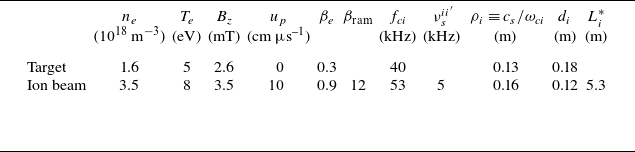The axial magnetic field $B_z$ is produced with an external Helmholtz coil pair and can reach 9.0 mT. A weak mirror field around the washer guns (mirror ratio of 3) is used to increase the plasma radius while avoiding a strong axial gradient to the field. Nominal experimental values are listed in table 1 for reference.

Table 1.

Plasma parameters on axis, and estimates of relevant frequencies and lengths. The ion interpenetration length $L_i^*$ is calculated as described by (1).

Table 1. Long description

A table comparing plasma parameters and relevant frequencies and lengths. The table has two rows and twelve columns. The columns are labeled as follows: n_e (10^18 m^-3), T_e (eV), B_z (mT), u_p (cm µs^-1), β_e, β_ram, f_ci (kHz), v_i^i’ (kHz), ρ_i ≡ c_s/ω_ci (m), d_i (m), L_i* (m). The first row is labeled ’Target’ and the second row is labeled ’Ion beam’. The values in the table are as follows: Row 1: n_e, 1.6; T_e, 5; B_z, 2.6; u_p, 0; β_e, 0.3; β_ram, 40; f_ci, 0.13; v_i^i’, 0.18; ρ_i ≡ c_s/ω_ci, 0.12; d_i, 5.3. Row 2: n_e, 3.5; T_e, 8; B_z, 3.5; u_p, 10; β_e, 0.9; β_ram, 12; f_ci, 53; v_i^i’, 0.16; ρ_i ≡ c_s/ω_ci, 0.12; d_i, 5.3.

With these three experimental knobs of $u_p$ , $n_e$ and $B_z$ , the plasma beta $\beta \equiv 2 \mu _0 n T / B^2$ and Alfvén Mach number $M_A \equiv u_p / v_A$ can be controlled. This control is not fully independent, as for non-zero $\beta$ the plasma diamagnetism weakens the field on axis due to the strong radial gradients (see subplots of figure 1). For low-frequency whistlers ( $\omega \lt \omega _{ce}/2$ ), such a configuration is well known to duct waves via refraction (Helliwell Reference Helliwell1965; Stenzel Reference Stenzel1999). This work differs from Stenzel’s comprehensive whistler research in a similar cylindrical geometry by our use of a high-beta compact-toroid piston, rather than strong radio-frequency fields, though many of the results are similar. While we explore a wide range of Alfvén ( $0 \leqslant M_A \leqslant \infty$ ) and sonic ( $3 \leqslant M \leqslant 6$ ) Mach numbers, the particular density and magnetic field strength presented in this paper are chosen for their clear whistler signals. For a nominal piston speed of $u_p = 100$ km s^–1, the experiment has $M_A \sim 2.4$ on axis but becomes sub-Alfvénic for $R\geqslant 0.45$ m.

The experimental measurements come from four hanging probes at fixed position and a movable probe that can be scanned over a region, as shown in figure 1. The four hanging probes are located at $Z = -0.88,-0.26,+0.52,+0.88$ m and $R = 0.15$ m, with the first and second pairs offset in the azimuthal direction by 60 $^\circ$ . Each hanging probe has four planar tips operated as two double probes measuring ion saturation current $I_{\textrm {sat}}$ and an orthogonal set of three $\dot {B}$ -coils, all digitised at 10 MHz. These double probes were developed for their resilience to the large plasma potential fluctuations intrinsic to the experiment. However, density measurements from the double probes are calibrated to the colder background plasma and likely overestimate $n_e$ elsewhere. The Langmuir/ $T_e$ probe is a 16-tip probe with a three-axis $\dot {B}$ -coil set capable of resolving the electron temperature and magnetic field up to 5 MHz. That probe scans the shaded region in figure 1, from $Z=-0.1$ to $+0.4$ m and $R = 0.0$ to $0.5$ m in 5 cm steps. Radial profiles of the target plasma for this primary scan are shown in figure 1(b).

While the target plasma and magnetic field are highly reproducible, the jitter in breakdown of the coaxial plasma gun leads to significant variability in the piston speed. To complete a scan, shots are taken at each $T_e$ probe location until a piston velocity of $u_p = 100\pm 10$ km s^–1 is observed, forming a dataset of around 200 shots, with two shots per location. Aligning data between shots requires offsetting in time for shot-to-shot jitter, and, in a few outlier cases, also multiplying the time axis by a factor $u_p / u_p^{\textrm {mean}}$ to correct for the speed.

Figure 2.

(a) Measurements of density $n_e$ and axial magnetic field $B_z$ , taken at $R=0.15$ m and offset in Z. The four colour points (red, blue, black and green) represent locations of peak density (piston centre), magnetic ramp (piston front), earliest density increase (ion beam front) and earliest coherent polarised signals (whistler front), with speeds shown in the upper right. At $t=12$ $\unicode{x03BC}$ s there is separation of multiple $c/\omega _{pi}$ between each. (b) Using data from a single radial scan at $Z=-0.1$ m, two-dimensional profiles of plasma potential $V_p$ , toroidal magnetic field $B_\phi$ and $n_e$ . Black contours are poloidal magnetic field lines. The dashed line follows the $V_p$ peak which forms half of the V-shaped potential. In the centre, the highest frequencies of the whistler pulse arrive at 4 $\unicode{x03BC}$ s. White contours on the bottom plot track where $n_e$ is 2, 3 and 4 times the initial radial value. The ion beam that arrives at 6 $\unicode{x03BC}$ s and $R\lt 0.2$ m is from focusing of reflected ions towards the axis.

Figure 2. Long description

Panel A: The left side of the panel shows a line graph depicting measurements of density at different positions along the Z-axis, with time on the horizontal axis. The right side of the panel shows another line graph depicting measurements of the axial magnetic field at different positions along the Z-axis, with time on the horizontal axis. The graph includes four color-coded points (red, blue, black, and green) representing locations of peak density, magnetic ramp, earliest density increase, and earliest coherent polarized signals, respectively. The speeds of these points are shown in the upper right corner. At 15 microseconds, there is a separation of multiple fronts between each point. Panel B: The top section shows a two-dimensional profile of plasma potential with radial position on the horizontal axis and time on the vertical axis. The middle section shows a two-dimensional profile of the toroidal magnetic field with the same axes. The bottom section shows a two-dimensional profile of electron density with the same axes. Black contours in all sections represent poloidal magnetic field lines. The dashed line in the top section follows the peak which forms half of the V-shaped potential. In the center of the middle section, the highest frequencies of the whistler pulse arrive at 4 microseconds. White contours on the bottom plot track where the electron density is 2, 3, and 4 times the initial radial value. The ion beam that arrives at 6 microseconds and 0.5 meters is from the focusing of reflected ions towards the axis.

To show the spatial and temporal development as the piston traverses the vessel, in figure 2(a) we plot data from the hanging probes as well as the $T_e$ probe. This plot uses five shots that measured a piston speed of $u_p \sim 85\pm 5$ km s^–1, slower than the 100 km s^–1 target but with a smaller variance. The $T_e$ probe is at the same radial location $R=0.15$ m as the hanging probes and is moved in Z between shots. The piston enters from the machine south pole at $Z=-1.5$ m (top of plot) travelling towards the north wall at $Z=1.5$ m (bottom). We identify the peak piston density in red and the axial field magnetic ramp in blue, which respectively mark the piston centre and leading edge. The earliest rise in density (black) and the earliest coherent whistler signals (green) are both propagating faster than the piston. When the first whistler signals reach the far wall at $t=12$ $\unicode{x03BC}$ s, the system has developed for $3\omega _{ci}^{-1}$ and each front is separated by several $d_i$ .

Figure 3.

(a) Hodograms from the Z = 0.52 m probe for two shots with the Helmholtz field direction flipped. The wave remains right-hand circularly polarised with respect to the field direction. Peak frequencies are above $20 \omega _{ci}$ . (b) Field $B_r$ traces from the Z = 0.52 and 0.88 m probes. The dotted lines estimate the phase velocity $v_{\textrm {ph}}$ while the dash-dotted line estimates the group velocity $v_{\textrm {gr}}$ from the earliest coherent polarised $r\phi$ signal, which is close to the expected $2 v_{\textrm {ph}}$ . Note also that the highest measured wavenumbers of ${\sim}5$ are less than the prediction of $2\pi$ . (c) The R-wave dispersion relation for $B_z = 2.4$ mT and $n_e = 1.6\times 10^{18}$ m $^{-3}$ . Crosses are values of $\omega$ and $k_\parallel$ measured from (b), with the Alfvén and piston speeds for reference.

Figure 2(b) shows the plasma potential, magnetic field and density from a radial scan of 11 shots from the 100 km s^–1 dataset. At top, a large V-shaped potential is marked with dashed lines, and a second, smaller potential can be seen on axis 5 $\unicode{x03BC}$ s ahead. In the centre, the toroidal magnetic field $B_\phi$ is plotted as a colourmap, along with poloidal field lines $B_{RZ}$ plotted in black. At bottom, the high-density piston collides with the target and produces a focused ion beam, visible from 6 to 11 $\unicode{x03BC}$ s and extending out to $R\sim 0.2$ m.

We unambiguously identify these early magnetic waves as whistlers from their right-handed polarisation, the factor of two difference between the peak phase and group velocities and their agreement with the R-wave dispersion relation (figure 3 c) (Chen Reference Chen2016). The right-handed polarisation is clearly seen in figure 3(a) whereby reversing the background magnetic field flips the rotation direction. In figure 3(b), the group velocity of the earliest coherent circularly polarised signals is roughly double the maximum measured phase velocity. The phase velocity measurements, taken from the local extrema in the $B_r$ time history, line up within measurement uncertainty along the R-wave dispersion relation in figure 3(c). The dot-dash line tracking the group velocity intersects the vessel wall at the same time as the piston enters. From this we infer that the whistler pulse is initiated as the very high- $\beta$ piston bursts into the vessel and bends the upstream field lines down to an ion-skin-depth-scale length.

Figure 4.

The $T_e$ probe time histories of density, temperature, plasma potential and magnetic field. These measurements are taken on the axis, but +20 cm further in Z from the data in figure 2(b). The error bars are estimates of the total systematic error including the Langmuir fitting routine, and not the much smaller standard deviation of statistical noise. The potential fluctuations from 23 to 27 $\unicode{x03BC}$ s are global ( ${\rm d}V_p/{\rm d}z = 0$ ), while the later fluctuations do indicate local electric fields.

Figure 4. Long description

The image contains two line graphs depicting the time histories of various plasma parameters. Panel A shows the electron density (ne) and electron temperature (Te) over time. The x-axis represents time in microseconds (t [μs]), ranging from 25 to 45 microseconds. The left y-axis represents electron density in units of 10^18 per cubic meter (10^18/m^3), and the right y-axis represents electron temperature in electron volts (eV). The black line represents electron density, while the red line represents electron temperature. The shaded areas around the lines indicate the estimated systematic error. Panel B shows the plasma potential (Vp) and the magnetic field components (Br, Bφ, Bz) over time. The x-axis is the same as in Panel A. The left y-axis represents the magnetic field in millitesla (mT), and the right y-axis represents the plasma potential in volts (V). The orange line represents plasma potential, the red line represents the radial component of the magnetic field (Br), the green line represents the azimuthal component (Bφ), and the blue line represents the axial component (Bz). The error bars are estimates of the total systematic error, including the Langmuir fitting routine. The potential fluctuations from 23 to 27 microseconds are global, while the later fluctuations indicate local electric fields.

This same field-line bending can be seen in the time history of the topmost magnetic trace of figure 2(a), which shows the sharpness of this bend 0.6 m away from the entrance at Z = –1.5 m. For this near step function in $B_z$ , the $B_r$ component is similar to a delta function of finite width of order $c/\omega _{pi}$ . We would expect that a Fourier decomposition then be limited to wavenumbers less than $k=2\pi /d_i$ . If we treat this initial perturbation as a large-amplitude whistler wave that disperses into the upstream (Krasnoselskikh et al. Reference Krasnoselskikh, Lembège, Savoini and Lobzin2002), this condition then provides a limit on the production of whistler waves in a piston-driven experiment: if the ramp thickness is limited by the ion skin depth, then waves above $k = 2\pi /d_i$ should not be generated. As expected, figure 3(c) shows that the highest measured wavenumbers of $k\sim 5/d_i$ are less than this limit.

More magnetic signals, here taken on axis, can be seen in figure 4 which shows time histories from the $T_e$ probe for a representative shot. The substantial $B_z$ fluctuations are not indicative of oblique propagation but are instead a feature of the wave solution to the cylindrical boundary conditions, akin to an $m=0$ Helicon mode (Chen Reference Chen2015). The small $B_r$ and $B_\phi$ signals are possibly contributions from $m \geqslant 1$ modes from a non-axisymmetric initial piston, a feature that is sometimes seen in fast camera images.

While the experiment’s large electron collisionality ( $\nu _{e0} \sim 5\times 10^{6}\ \textrm{s}^{-1} \gg \tau _{\textrm {exp}}^{-1}$ ) is typical of laboratory plasmas, a high thermal electron collisionality does not preclude collisionless ion behaviour or even acceleration of energetic electrons (Park et al. Reference Park2015; Fiuza et al. Reference Fiuza2020). We calculate ion interpenetration lengths $L_i^*$ following laboratory plasma jet experiment convention (Messer et al. Reference Messer, Case, Wu, Brockington and Witherspoon2013; Merritt et al. Reference Merritt, Moser, Hsu, Adams, Dunn, Miguel Holgado and Gilmore2014):

(1) \begin{equation} L_i^* = \frac {u_p}{4\nu ^{ii'}_s + \nu _s^{ie'}}, \end{equation}

where the $\nu _s$ terms are the slowing rates as described in Huba (Reference Huba2013). As shown in table 1, we estimate $L^*_i$ for an upstream particle colliding with the beam to be 5.3 m, which is much larger than the 3 m vacuum vessel. While this suggests that the ions are effectively collisionless, the electrons are everywhere collisional and magnetised ( $\omega _{ce} \gg \nu _e \gg \tau _{\textrm {exp}}^{-1}$ ). This limits comparison with space plasmas like magnetospheric bowshocks, where electrons are generally collisionless on scales much larger than any shock transition layer.

The concave-forward potential structure reflects ions in an on-axis beam which is visible in figure 2(b) from 6 to 11 $\unicode{x03BC}$ s and $R\leqslant 0.2$ m. This moving potential jump is larger than the relative ion kinetic energy $K_i = m_i u_p^2 /2 = 52$ eV for $u_p = 100$ km s^–1 and so can reflect ions. That the beam travels slower than $2 u_p$ and that the density increase exceeds two suggest that this is not perfect specular reflection. It is important to understand if this discrepancy is due to dissipation and shock heating, or some other more benign effect.

To investigate this further, we performed a basic Monte Carlo simulation of single-particle ion trajectories in the piston reference frame. We began by recognising that the two-dimensional temporal plots in figure 2(b) cannot be simply converted to spatial plots with the Taylor hypothesis because of both the changing velocity and also the dynamic evolution of the structures. Instead, we use the time history of the measured phase velocity from figure 2(a) to reconstruct the spatial structure. The resultant static electric and magnetic field structure is used to simulate the trajectories of $10^5$ ions with an initial 2 eV thermal distribution impinging at –100 km s^–1. The spatial and velocity distributions from this simulation are shown in figure 5. While this model ignores the time evolution of the structure, qualitatively it reproduces the compression in the density by a factor of ${\sim}2.4$ and shows a perpendicular ion-beam temperature of $T_\perp \sim 8.6$ eV. These results show that this geometric effect of a concave-forward potential structure can lead to on-axis compression that naively resembles shock compression above the factor of 2 expected for purely reflected ions.

Figure 5.

Results from a simple Monte Carlo simulation with 10 000 test particles launched towards the static potential derived from the top plot of figure 2(b). This simple model roughly reproduces the observed density compression in the reflected ion front.

The leading edge of the ion beam satisfies the cyclotron resonance condition with the adjacent whistlers (Gary Reference Gary1991):

(2) \begin{equation} \omega - {\boldsymbol k \boldsymbol{\cdot }\boldsymbol{v}_{\textrm {beam}}} \pm m \omega _{ci} = 0, \end{equation}

where $m$ is the harmonic number. Using the wavelength $\lambda$ at the leading edge of the beam measured from the $B_r$ signals in figure 3, we find for $m = 1$ that $(\omega -m\omega _{ci})/ $ $ k=11\pm 1$ cm $\unicode{x03BC}$ s^–1. This is resonant with the beam velocity $v_{\textrm {beam}} = 13.3$ cm $\unicode{x03BC}$ s^–1 within a thermal speed ( $v_{thi} = 2.0$ cm $\unicode{x03BC}$ s⁻¹ at 2 eV). However, the ion beam is well separated from the piston for only 5 $\unicode{x03BC}$ s $\sim \omega _{ci}^{-1}$ , which is likely too short for substantial beam–wave coupling (Onsager, Winske & Thomsen Reference Onsager, Winske and Thomsen1991). Beam–wave coupling could appear as growth of the amplitude of the plasma potential collocated with the axial magnetic field rarefactions, shown in figure 4 at 30 and 32.5 $\unicode{x03BC}$ s. Given the short duration, we believe we are only seeing the dispersion of the initial steep piston ramp and cannot claim that the whistler waves grow or damp on the ion beam.

Summarising this experiment, we observe the simultaneous production of whistler waves and Doppler-shifted cyclotron resonant reflected ions. To restate the mechanism, a high-pressure supersonic piston creates a steep magnetic ramp and a large plasma potential jump. This sharp magnetic feature disperses into super-Alvénic whistler waves. At the same time, the strong plasma potential jump at the piston front specularly reflects ions. These reflected ions are in Doppler-shifted cyclotron resonance with certain whistler wavenumbers and could lead to growth of the whistler wave train, though we do not observe this given the short experiment duration. We reiterate that while the density compression of these reflected ambient ions naively satisfies the Rankine–Hugoniot conditions of a developed shock, this is early in the shock development stage and the ion-reflecting surface has not detached from the piston.

Producing a fully developed shock with the expected Rankine–Hugoniot jump conditions is difficult at these plasma parameters. The prerequisite step of shock detachment, where the potential structure in the leading magnetic field rarefaction grows until it can independently reflect ions, will likely require tens of ion cyclotron periods Onsager et al. (Reference Onsager, Winske and Thomsen1991). Experimentally, this would mean either increasing the magnetic field to extend the effective duration of the experiment such that $L_{\textrm {exp}}/u_p \gg \omega _{ci}^{-1}$ , or repeating this experiment on a larger device. The first option would also require quadratic increases in background density and piston ram pressure to keep $\beta$ and $M_A$ constant. In either case, maintaining the collisionless ion condition of (1) would be difficult.

An additional experimental challenge is how to inject enough energy into the piston to be effective for the duration of the experiment. As the piston enters the main vessel and expands, its internal pressure drops adiabatically. This is reflected in the decreasing peak piston density in figure 2(a), which is above $10^{20}\ \textrm {m}^{-3}$ at the first probe and drops to $10^{19}\ \textrm {m}^{-3}$ at the second probe 0.5 m later. When the internal pressure has dropped below the ram pressure $2m v_i^2$ equivalent, the piston is no longer effective. To keep the internal pressure above the ram pressure for the entire duration is a demanding requirement for a pulsed power system on this scale.