1 Introduction
It is well known that optimally designed intergenerational risk sharing (IRS) is potentially welfare improving for an economy with overlapping generations under uncertainty (Gordon and Varian, Reference Gordon and Varian1988; Shiller, Reference Shiller1999; Weil, Reference Weil2008). However, the private market fails to provide insurance products based on IRS as human capital is non-tradable and current generations cannot sign contracts with future generations. Governments can implement institutional arrangements that enable generations to share risk amongst each other via fiscal policy and public debt management.Footnote 1 Due to longevity and population ageing, the sustainability of the existing public programs is under pressure. Recently, the large government budget deficits – as a result of the financial crisis – load further pressure on the viability of public programs. Therefore, many countries are gradually reducing (or planning to reduce) PAYG social security and promoting the individual defined contribution saving schemes (Feldstein, Reference Feldstein2005; Diamond and Orszag, Reference Diamond and Orszag2005). The rapid growth of individual DC schemes and the likely decrease of public programs raise the question as to how to maintain a desirable level of IRS.
The government might not be the only institution to implement IRS. Funded pension schemes with mandatory participation are able to implement IRS as well. In this paper, we investigate whether IRS is desirable in funded pension schemes and, if so, what the optimal design regarding risk-sharing rules should be. Due to their long-run nature and mandatory participation rules, funded pension schemes seem natural candidates to organize IRS. The literature on IRS primarily focuses on the design of contingent social security and on the optimal combination of PAYG and funded system in order to share unanticipated economic shocks. We add to the literature by examining the real, existing forms of funded pension systems, and derive the optimal design of IRS in the funded systems. To make the analysis realistic, we extend the often-used two-period overlapping generation model to 55 annual periods. Furthermore, in addition to the welfare analysis, we also look at the market value of implied value transfers of risk sharing.
There are a number of differences between our paper and the existing literature. Allen and Gale (Reference Allen and Gale1997) and Gollier (Reference Gollier2008) study the role of shareholder-sponsored financial intermediaries (or corporate-sponsored pension funds) in facilitating intertemporal risk smoothing. They find large welfare improvements if shareholders are able to contribute or accumulate sufficiently large financial buffers as means for intertemporal smoothing. Importantly, they point out that, without mandatory participation, the system will break down and go back to the market solution once the buffer is exhausted or becomes insufficient. The collective schemes with mandatory participation (as in this paper), however, avoid the system breakdown. Van Bommel (Reference Van Bommel2007) argues that intergenerational risk sharing might not be sustainable when the fund is overfunded, as living generations might renegotiate and raid the surplus.
Our main findings are the following. Firstly, from the entry cohort point of view, well-designed realistic collective pension schemes can be welfare improving over the optimal individual life-cycle benchmark. Despite the fact that risk-allocation rules and asset allocation are assumed to be constant over the life-cycle, the optimal collective scheme outperforms the individual benchmark. The best-performing collective scheme in the standard setting, for example, leads to a 2.3% increase in certainty-equivalent consumption per annum as compared to the optimal individual pension scheme. The key intuition is that the long-term nature of the collective pension funds allows for smoothing of risks across many generations. By allowing transfers across generations in addition to absorbing risks through out one's life time, IRS adds one degree of freedom compared to the individual scheme. Therefore, risk sharing across generations is welfare enhancing for all from an ex ante perspective. Moreover, efficient risk sharing should involve both retirees and current and future workers, so that risks are more evenly spread among all stakeholders. For instance, a hybrid pension plan, which adjusts both contribution and benefit levels to absorb funding risks, is the most preferred in welfare terms. It outperforms plans that only allow for adjustments in either contributions or benefit levels.
Secondly, intergenerational risk sharing increases the risk-bearing capacity of the economy and hence increases the demand for risky investments. When comparing the asset allocation of IRS embedded collective schemes with that of the individual scheme, the portfolio weight in equities are higher for the collective schemes on average. Across the collective schemes, the hybrid scheme with more efficient risk sharing chooses the most aggressive portfolio. In other words, participants are more able to exploit the positive equity premiums by taking more risk. This finding confirms former results of Campbell and Nosbusch (Reference Campbell and Nosbusch2007) and Gollier (Reference Gollier2008).
Thirdly, the recognition of the welfare aspects of risk sharing within pension funds is important. An analysis in terms of only market value may easily lead to the spurious conclusion that pension funds are irrelevant, as argued for example by Exley (Reference Exley2004). The market valuation of IRS shows that the risk-sharing arrangement is a fair deal when the fund is initially 100% funded. In other words, the market value of funding surplus equals the market value of the deficits in the generational account of the entry cohort. However, the schemes with IRS are potentially welfare enhancing, and thus a positive-sum game in welfare terms. An agent joining an underfunded collective scheme is not necessarily worse off in welfare terms. It is possible for well-structured pension schemes to absorb funding deficits up to 10–20% by a combination of higher contributions and benefit cuts over a number of years and still enhance the welfare for participants. Furthermore, the welfare gains for the new entry cohort are not at the cost of older and future cohorts. From an ex-ante point of view, the expected welfare of future cohorts is even higher compared to the currently entering cohort. Although optimization occurs by the entering generation, the fund is expected to build up a buffer, and is, in expectation, overfunded in the long run.
For a realistic description of the economy and individual's life cycle, this analysis is set in a partial equilibrium framework. We should keep in mind some likely general equilibrium effects. In a general equilibrium setting, the re-design of pension system (including IRS) is likely to affect capital accumulation, asset prices, and economic growth in a long run. Since the IRS is implemented through funded pension schemes instead of the PAYG system, the typical ‘capital crowding out’ effect of the PAYG system is absent in our setting. Asset prices will be endogenous in a general equilibrium setting, depending on supply and demand. Our paper shows that IRS increases the risk-bearing capacity of the economy and so the demand for risky assets ceteris paribus. In the general equilibrium setting, Campbell and Nosbusch (Reference Campbell and Nosbusch2007) show that the asset prices and risk premiums are likely to be reduced, assuming a fixed supply of risky assets. We therefore also analyze the welfare implication under reduced equity risk premium and provide additional robustness checks.
The paper is organized as follows. Section 2 describes the structure of the economy, the preferences of the pension scheme participants, and the structure of the pension arrangements. Section 3 evaluates the welfare outcomes of the various pension schemes. Section 4 discusses the robustness of the results and Section 5 looks at the implications for future cohorts. Section 6 concludes.
2 Model
The schemes we analyzed are stylized versions of collective (industry or public sector) pension funds operating in countries such as the US, UK, Canada, and the Netherlands. A key feature of these schemes is that they are able to smooth shocks over and beyond the lifetime of a single generation. In these collective schemes, assets are pooled and owned collectively and invested in the financial markets, typically partly in risky assets (stocks) to capture the equity premium. Liabilities are defined-benefit-like. Fluctuations in asset returns lead to mismatch risk between the pension funds' assets and liabilities. Surpluses or deficits in the funding process are shared among young, old, and future generations by adjusting either contributions, benefit levels, or both, which leads to intergenerational transfers. Ex ante, contributions are set such that in expectation, a new entry generation funds its own pension. Ex post, a given generation may be a net payer who leaves a surplus for future generations, but also may be a net receiver who leaves a deficit for future generations. In this way, unanticipated investment risks can be shared among many generations over a long period of time. In this paper, we investigate whether such collective pension schemes can be welfare improving over the optimal individual benchmark.
Unlike the two-period OLG models, this paper specifies realistic collective pension schemes consisting of 55 overlapping generations (with 40 working cohorts and 15 retiree cohorts in each period). The pension funds invest the savings of all cohorts in one asset pool, and part of it may be invested in the stock market. The return on the risky asset is exogenous. The key issue here is to determine who of the stakeholders, when, and to what extent they should take part in risk bearing. We therefore specify three schemes according to their risk-allocation rules. In a defined benefit scheme with contribution adjustment, the workers bear the funding risks, whereas in a defined benefit scheme with benefit adjustment, the retirees bear the funding risks. In the hybrid defined benefit scheme, both workers and retirees bear the funding risks.
After describing the economy in Section 2.1 and optimal individual scheme in Section 2.2, we focus on the funded pension schemes with IRS in detail in Section 2.3. The schemes are then optimized with respect to the risk-allocation rule and the investment policy, both from the point of view of a newly entering cohort, as well as from the point of view of a social planner who takes the utility of future generations into account. We also examine the market value of contributions and benefits derived from the optimal schemes, to make sure that the schemes are actuarially fair. This means that, ex ante, each generation finances their own pensions, and there is no deterministic wealth transfer in the system a priori.
2.1 Economy, overlapping generations, and preferences
Two asset classes are traded in the financial market: a risky stock portfolio and a risk-free asset. For simplicity, we assume that the interest rate, r, is non-stochastic. Stock prices follow a geometric Brownian motion with a constant drift μ. The investment portfolio is a mix of stocks and risk-free assets, with portfolio weight ωt for stocks. The dynamics of this asset portfolio are given by

where σ is the volatility of stock returns. Both the expected return and the volatility increase linearly with the fraction ωt invested in equities. The Sharpe ratio of the investment portfolio equals

The stochastic discount factor M t in this economy is the deflator for risky cash flows, which in our model evolves according to

This deflator can be used to calculate the market value of stochastic pension contributions and benefits in Section 3.
The default values for the model parameters are in line with the values used in the recent literature. We assume the (real) interest rate is constant and equals r=2%. The expected (real) return on stocks is assumed to be μ=6%, implying an equity premium of 4%, which is in line with the long-run estimates in Fama and French (Reference Fama and French2002). The volatility of stock returns is σ=15%, which is close to the value (15.7%) estimated by Cocco et al. (Reference Cocco, Gomes and Maenhout2005).
We consider an economy populated by 55 overlapping generations (from age 25 to 80). We assume that all individuals start working at age 25 (t=0), retire at age 65 (t=R=40), and die at age 80 (t=T=55). During the first 40 years, people work and earn a flat real labor income, which is normalized to 1.Footnote 2 The population (as well as the collective pension fund) has stationary age composition. During the retirement period (R⩽t<T), the individuals receive no income but consume their accumulated pension wealth, denoted by W t. Apart from the pension wealth, there are no savings. The 55 homogeneous cohorts have the same population size and share the same preferences. Individuals have a constant relative risk aversion (CRRA) utility function defined over a single non-durable consumption good. Let c t denote the consumption level at time t, then the individual's preferences are defined by
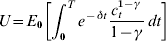
where γ is the risk aversion parameter and δ is the subjective discount rate. In the baseline setup, we set the subjective discount rate equal to δ=4%, and the risk aversion parameter γ=5 for a typical individual. In the robustness checks, we allow for a lower equity premium and different values of δ and γ.
2.2 Cohort specific pension schemes
As the benchmark, we consider the optimal individual (OI) scheme, where the individual bears all the non-diversifiable investment risks and there is no intergenerational risk sharing. The individual can optimally choose his consumption level and portfolio composition (under short sales and borrowing constraints) at any time throughout his life.
During the working period, the investor receives his labor income, which is normalized to 1. The individual chooses his consumption stream c t optimally at every point in time, and invests the rest in financial markets. After retirement, the individual optimally consumes his wealth. The individual is free to choose the portfolio weight of stocks ωt continuously, within the constraints 0⩽ωt⩽1. Formally, the individual's consumption and portfolio choice problem is characterized by the following objective function

and subject to the pension wealth dynamics



where W tOI is the accumulated financial wealth in the OI scheme.
Because of the short-selling and borrowing constraints, no analytical solution is available. We use dynamic programming to solve for the consumption and investment in the optimal individual scheme. We use the numerical procedures presented by Carroll (Reference Carroll2006) to solve for the optimal consumption and portfolio policy before retirement, under the borrowing and short-selling constraints, 0⩽ωt⩽1. Details of the solution method are given in the Appendix.
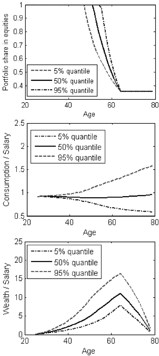
Figure 1 shows the life cycle quantile distributions (at 5%, 50%, and 95% quantile levels) of portfolio weight, consumption, and wealth accumulation of the optimal individual scheme for a benchmark investor (γ=5, δ=4%). The distribution of portfolio choices (ωt) is shown in the top panel of Figure 1. On average, the optimal portfolio weights are decreasing with age. As explained by Campbell and Viceira (Reference Campbell and Viceira2002), this is due to the leverage effect of human capital (or to be precise, the present value of future pension contributions). The desired equity exposure in total wealth, including financial wealth and human capital, is constant over the life cycle. Individuals achieve the desired equity exposure of their total wealth by adjusting their financial portfolio.
Life cycle profiles of the optimal individual (OI) scheme
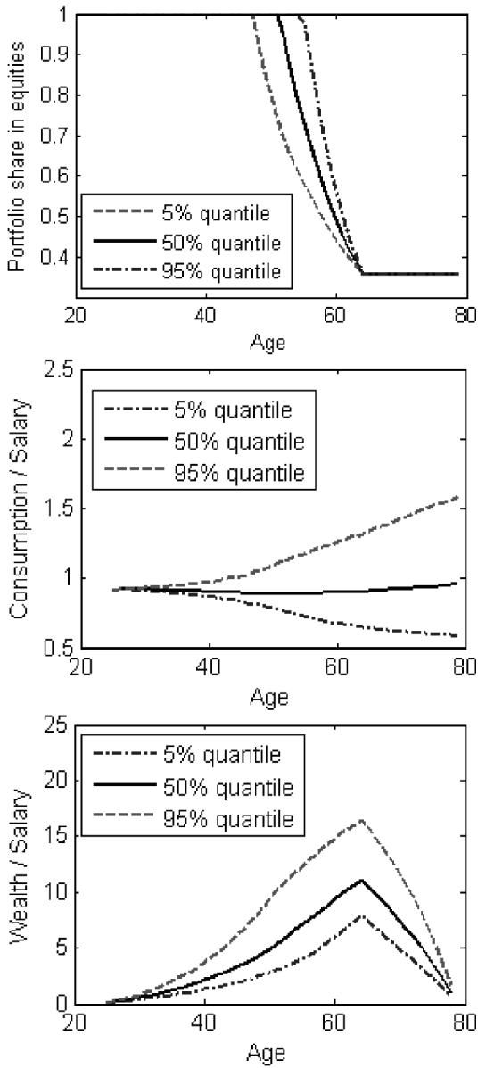
The distribution of consumption (normalized by income) for the baseline parameters is shown in the middle panel of Figure 1. The median consumption level is relatively flat over the life cycle, but uncertainty in old-age consumption is increasing with time. In the OI scheme, the consumption is higher (hence new saving is lower) when the financial wealth is boosted by good returns. Finally, the accumulated assets over the life cycle are presented in the lower panel of Figure 1. These asset values show wide dispersion. They peak at the retirement date with a median amount standing at around 11 times the annual labor income.
2.3 Pension schemes with intergenerational risk sharing
In this section, we model collective pension schemes that allow for intergenerational risk sharing. Mandatory participation is required by law and the agents are not allowed to save or borrow outside the pension fund (this restriction will be relaxed in Section 4.3). We first define the targeted pension benefit and contribution policies for such funds, and then specify the risk-allocation rules, which adjust the benefits and/or contributions as functions of funding surplus. Finally, the design parameters are optimized with respect to a chosen objective.
2.3.1 Pension liability
Since the collective pension schemes considered in this paper are certain variants of defined benefit (DB) schemes, we shall start with traditional DB schemes to introduce the target liability, target benefit, and contribution rates. In a traditional average salary defined benefit scheme, the retirement benefit is a fixed fraction (the so-called replacement rate) of labor income during the working period. These pension benefits are funded by the contributions plus investment proceeds. The higher the pension ambition, the more contributions are required. The actuarially fair contribution principle requires that ex-ante each generation finances its own pension; that is, the market value of the contributions equals the market value of the benefits. The actuarially fair contribution rate can be solved from the following present value equivalence
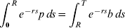
where b denotes the target benefit and p the target contribution (recall that we have normalized the flat real labor income to 1). For each age cohort, denoted by x, the target DB liability equals the difference between the present value of risk-free benefits and the present value of yet-to-be-paid risk-free contributions

At the aggregate level, the target liabilities of the fund can be calculated simply as the sum of the liabilities for each age cohort, with the size of each cohort normalized to 1.

Given the stationary age composition of the fund and the fixed target benefit level, the target liability L is time invariant. If the fund invests fully in the risk-free asset, then the actual liability follows exactly as the target liability L. If the fund accepts mismatch risk, for example by investing in stocks, there may be funding surpluses or deficits with respect to the target liability. Let A t denote the value of the pension fund's assets, which starts off with an initial asset value of A 0=FR 0⋅L, where FR 0 is the initial funding ratio. Let ω denote the fraction of assets invested in risky assets. The portfolio weight ω is time invariant and the same for each cohort in the fund.Footnote 3 Then, the fund's assets follow the dynamics

where p t and b t denote the actual contribution and benefit levels which will be specified shortly. The fund has 40 contributing cohorts and 15 benefit receiving cohorts. In most of the experiments, we assume FR 0=1, but we shall show some results with initial over- or underfunding. The fund surplus is defined as the difference between assets and the target liability level

Notice that the collective pension schemes may leave surpluses or deficits at the end of the first cohorts lifetime (i.e. at t=T). These lead to intergenerational transfers and hence to intergenerational risk sharing. Equation (9) imposes that the present value of the target premiums and benefits are equal, so that Ponzi schemes are explicitly excluded. We provide a deeper analysis of the value of the intergenerational transfers in Section 3.3.
2.3.2 Risk-allocation rules
If the investments of the fund were completely risk free, there would never be any overfunding or underfunding. However, with a risky investment policy, or other sources of systematic risks, the mismatch risk has to be allocated in some way. This is done by adjusting contributions p t and benefits b t as a function of the fund surplus S t and the target contribution (p) and benefit (b). This adjustment scheme is motivated by real-world examples.Footnote 4 We now discuss three stylized schemes, which differ in their risk-allocation rules. These risk-allocation rules specify who of the stakeholders, when, and to what extent they are taking part in risk bearing.
In the defined benefit with contribution adjustments (DBCA) scheme, benefits are fixed at b t=b, but contributions are adjustable. So, the working cohorts bear all the funding risk. We specify a simple contribution policy, where contributions per cohort are a function of the target contribution level p and the funding residual per cohort S t/R

The slope coefficient α determines the speed of absorbing the funding imbalances. The choice α=1 implies that a funding imbalance is immediately and fully absorbed. A lower value of α implies that part of the funding residual is shifted to the future, and shared across generations.
In the defined benefit with benefit adjustments (DBBA) scheme, contributions are fixed at p t=p, but benefits are adjustable in order to absorb the funding surplus. In this scheme, retired cohorts bear the funding risk, where benefit per retired cohort are a function of the target benefit level b and the funding residual per cohort S t/(T−R)

Again, the lower the value of β, the higher the degree of intergenerational risk sharing.
The hybrid defined benefit (DBH) scheme adjusts both contributions and benefits simultaneously to absorb the funding residual. The contribution and benefit are linearly related to the funding residual S t. More specifically, a fraction α of the funding residual is shared among employees and a fraction β of the funding residual is shared among retirees


Under this rule, consumption before and after retirement is related to the funding surplus. This resembles the optimal consumption rule in the classical consumption and portfolio choice problem in the spirit of Merton (Reference Merton1969) where the optimal consumption is linearly related to wealth.
The following table summarizes the differences among the collective schemes:

When α+β approaches the risk-free rate r, each generation in each period absorbs only the ‘interest’ accrued on their funding residual and passes the principal into the infinite future. To get stability over time (i.e., non-explosive values for the surplus), we need to restrict α+β>r.
2.3.3 Pension policies optimization
We optimally choose the target contribution rate (p) together with the risk-allocation rule (α,β) and investment policy (ω), based on the expected life-time utility of the 25-year-old entering participants; that is, the policy parameters {p,α,β,ω} of the three collective plans are optimized from the perspective of the cohort entering at time t=0. Therefore, the specification of the utility function of the pension fund is the same as in the individual case, equation (5). The optimization problem of the pension fund then becomes
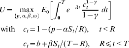
subject to the wealth dynamics (11). Since the pension fund is borrowing and short-sale constrained, the portfolio choice is constrained by 0⩽ω⩽1. The actual contributions and benefits (p t, b t) follow directly from the risk-allocation rules (15), (16) in different schemes. The decisions {p,α,β,ω} are time invariant. The optimization problem therefore is static and can be solved using Monte Carlo simulations combined with a standard grid search in four dimensions. The Appendix gives more details about the optimization procedure.
3 Evaluation of pension schemes
Is intergenerational risk sharing desirable in funded pension system? If so, in what form? In this section, we evaluate the performance of the optimal individual and collective schemes. First, in Subsection 3.1, we compare the investment policies and consumption outcomes. Subsection 3.2 then provides a welfare comparison of the optimal collective schemes with the individual benchmark. Subsection 3.3 studies the intergenerational risk sharing in the collective pension schemes.
3.1 Optimal pension schemes
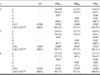
Table 1 reports the optimal design parameters {p,α,β,ω} for the pension schemes under the default parameter values (r=2%, δ=4%, μ−r=4%, γ=5). All schemes are initially fully funded (i.e. A 0=L).
Optimal pension schemes
The table shows the optimal pension scheme parameters under the default values for the time preference (δ=4%) and equity premium (μ−r=4%). The optimal contribution rate and the corresponding replacement ratio are given by (p,b). The optimal speed of risk absorbing by adjusting contributions or benefits is determined by (α,β) respectively. The optimal portfolio weight in equities is given by (ω). The welfare levels achieved under these optimal collective schemes are indicated by CEC (in units of annual salary). The ratio CEC/CEC OI shows the relative welfare gain or loss of the collective schemes relative to the optimal individual scheme (OI).

We find that institutional settings have a significant impact on the optimal contribution rates and investment policies. The target level of contribution p and portfolio choice ω vary significantly across schemes. The optimal target contribution rate in the DBCA scheme is the highest, requiring 16.6% of annual salary. This leads to the highest target replacement rate of 78.4% after retirement if the assets are invested fully risk free. The desired contribution rate in the DBBA scheme is the lowest among the collective schemes, requiring 13.1% of salary. Consequently, its target replacement rate b is also the lowest at 53.6%. The hybrid scheme DBH requires 14% of salary as the contribution rate and leads to a 66% target replacement rate. The actual contributions and benefits are different from these risk-free levels, as the pension fund can run surpluses or deficits.
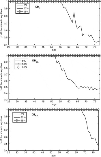
The portfolio choice of the DBBA scheme is less aggressive than the other collective schemes. The risky portfolio weight of the DBBA scheme is 60%, whereas the risky share of DBCA scheme reaches 96%. The hybrid scheme DBH accommodates the most aggressive investment portfolio, namely 100% in stocks. Comparing with the portfolio choices in the optimal individual schemes (Figure 1), where the stock portfolio share declines to 35% over the life cycle, the stock allocations of collective schemes are much higher. This shows that intergenerational risk sharing makes an aggressive investment policy more attractive. Due to intergenerational risk sharing, participants are more capable of exploiting the positive equity premiums. This finding confirms the results of Gollier (Reference Gollier2008) that intergenerational risk sharing increases the demand for risky investment. The values of the contribution and benefit adjustment parameters α and β are typically small, indicating that funding mismatches are absorbed gradually over time.
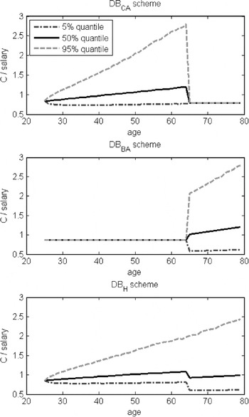
Figure 2 provides some graphical insight into the distribution of consumption over time. The figure plots the 5%, 50%, and 95% quantiles of the normalized consumption, c t, of the optimal collective plans, with the scheme parameters set corresponding to Table 1 with γ=5. In general, the consumption profiles are upward sloping with age. The distributions of consumption indicate that contribution reductions are more frequent, and also larger, than contribution increases. This is due to the positive equity premium. The figure shows that the hybrid scheme (DBH) is much better in distributing shocks over the full lifetime of the individual than the other collective schemes, where there are large fluctuations in consumption either just before retirement (DBCA) or during the retirement period (DBBA). This demonstrates that more efficient risk sharing can be achieved by using more risk absorbers. Through adjusting both contribution and benefit policies, the DBH scheme spreads the funding residual over both workers and retirees, i.e. all cohorts are involved in the risk sharing. From the risk-allocation perspective, DBCA and DBBA represent two extremes, with one group of people bearing all risks, while the other group is fully insured. The hybrid scheme allocates the risks more efficiently among all generations, hence reducing the costs of risk taking and resulting in welfare improvements.Footnote 5
Consumption profiles obtained from the collective schemes

3.2 Welfare evaluation
We use certainty equivalent consumption (CEC) as the welfare measure to gauge the performance of collective and individual pension schemes. The CEC can be computed easily from the following equality
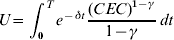
The most important result in Table 1 is the welfare levels of the optimized pension schemes from the entry cohort perspective. Welfare level is reported as the normalized certainty equivalent consumption in units of annual salary, CEC. Let CEC OI denote the welfare level achieved by the optimal individual scheme (OI). The ratio CEC/CEC OI then shows the welfare of the collective schemes relative to this optimal individual benchmark.
For participants with a default risk aversion (γ=5), the hybrid defined benefit (DBH) scheme provides a welfare gain of 2.3% per annum vis-à-vis the OI scheme in terms of certainty equivalent consumption. Over the full life-cycle, this amounts to more than one annual salary gain. The results indicate that well-structured intergenerational risk sharing is welfare enhancing compared to the optimal individual scheme. Despite the fact that adjustment speed coefficients and asset allocation are fixed, the hybrid collective scheme still outperforms the individual benchmark. The hybrid pension plan with flexibility in adjusting both contribution and benefit levels to absorb funding residue is the preferred one in welfare terms. It outperforms collective plans that only allow for adjustments in either contributions or benefit levels. Particularly, the DBCA scheme has a welfare loss of 0.3% relative to the optimal individual scheme, whereas the DBBA scheme shows a welfare loss of 2.7%.Footnote 6
3.3 Market valuation of the pension schemes
In this section, we focus on the market values of intergenerational risk sharing, through investigating the market value of contingent contributions and benefits in the optimal collective schemes. For an individual member, it may be difficult to trade his pension claims once he stepped into a pension contract, but a market valuation is useful ex-ante to evaluate a given pension deal. Furthermore, it is important to investigate whether the target contributions and benefits set according to equation (9) and the risk-sharing rules in equations (15) and (16) are actuarially fair. If so, then it means the market value of contributions equals the market value of benefits, and hence the scheme is a fair deal.
From the perspective of a new pension fund member, the market value of the pension deal is the value of the actual benefits minus the contributions. We take all the (stochastic) cash flows (p t, b t) generated by the optimal pension schemes and value them using the deflator method.Footnote 7 For the typical member with retirement date R and life expectancy T, the net present value (NPV) of the pension deal is the difference between the present value of benefits (PVB) and the present value of contributions (PVP)

where p t and b t are the (stochastic) actual contributions paid and benefits received, and M t is defined as in equation (3). From an ex-ante point of view, the pension scheme is a fair deal if the NPV is zero.
The collective schemes may shift the funding mismatches beyond one's life time, leaving surplus or deficit in the notional cohort account. An alternative way of calculating the present value of pension deals therefore is to look at the remaining balance left in the notional cohort account at the end of life of a cohort. A positive remaining balance indicates positive transfers from this generation to other cohorts. Similarly, a negative transfer means the cohort receives cash flows from other cohorts. In a collective pension scheme, any cohort writes a call option to share a funding surplus with the other cohorts, and holds a protective put option to receive protections from the other cohorts. When the value of the call equals the value of the put, the pension deal is a fair deal in value terms ex ante. Formally, let a t denote the accumulated asset in the notional cohort account through out their life time (0⩽t⩽T). Each cohort starts its notional account with no surplus or deficit, i.e. a 0=0. The dynamics of the cohort account are

Integrating out this dynamics and applying equation (21), the NPV of the pension deal can be decomposed as the sum of the value of the call and the put option, valuing the positive and negative transfers to other cohorts

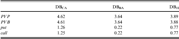
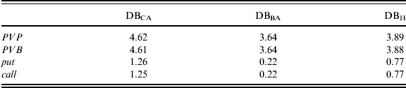
Table 2 summarizes the market valuation of the intergenerational transfers and options for initially fully funded pension schemes (FR 0=1). As required by actuarial fairness, the NPV is indeed zero for all collective schemes, i.e. market value of contributions equals the market value of benefits. It shows that the risk-sharing arrangements are fair deals when the fund is initially 100% funded. Ex ante, the starting generation does not borrow from future generations and therefore there is no ‘chocolate paradox’ of the type described by Shell (Reference Shell1971). However, the market values of positive and negative transfers (the implicit call and put options) are potentially large, between 0.2 to 1.25 annual salaries, indicating a substantial amount of ex post transfers. The magnitude of the transfers depends on the chosen asset mix, the level of contributions, and the risk-sharing rules. The DBCA scheme results in the highest value of transfers, whereas the DBBA scheme results in the lowest value of transfers. This makes the DBCA system less sustainable than the DBBA system, as future generations can be confronted with larger deficits in the pension fund.Footnote 8
Market value of intergenerational transfers
This table reports the market value of the actual contributions (PVP) and benefits (PVB) for a new entry cohort and an initially fully funded pension scheme (FR 0=1). The market value of the intergenerational transfers are shown in columns ‘call’ (for positive transfers) and ‘put’ (for negative transfers), as defined in equation (21). The market values are expressed in terms of multiples of annual salary.
4 Robustness checks
We now perform some robustness checks to see if our results still hold under different risk and time preferences, and with a reduced equity premium. Since this paper focuses on intergenerational risk sharing, we leave out the discussion on intragenerational risk sharing among co-existing generations with different preferences.
4.1 Risk aversion, time preference and equity premium
The degree of risk aversion has several effects on the optimal pension design, as shown in Table 1. Comparing the results as the coefficient of risk aversion increases from γ=3 to γ=8, we observe three changes: (i) the portfolios become less risky, (ii) the contribution rates increase, and (iii) the schemes rely more on intergenerational risk sharing by choosing lower values for α and/or β. Furthermore, the degree of risk aversion affects the welfare gain from intergenerational risk sharing. The welfare gain for a less risk-averse investor (γ=3) is 3.9% in the DBH scheme, whereas it is reduced to 0.9% for a more risk-averse investor (γ=8). The result that the more risk-averse agent obtains less welfare gain may seem counter-intuitive at first sight, but observe that the less risk-averse agent is willing to accept a more risky portfolio and thus benefits more from intergenerational risk sharing. The less risk-averse participants are also willing to accept larger adjustments in contributions and benefits in order to absorb funding mismatches, which is reflected in higher values for α and β.
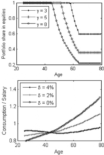
The degree of risk aversion has a major impact on the portfolio choice. Figure 3 displays the average life cycle portfolio profiles for investors with different risk aversion γ=3, 5, and 8. The less risk-averse investor allocates more assets in equities. The degree of risk aversion has only a minor impact on consumption and asset accumulation profiles, via the different portfolio choices. Highly risk-averse individuals save more and consume less compared with the less risk-averse individuals.
The impacts of different risk aversion and subjective discount rates on individual schemes

Figure 3 also shows the average life cycle consumption profiles for investors with different subjective discount rates δ=4%, 2%, and 0%. The subjective discount rate has a strong impact on consumption profiles. In general, from the first-order condition for optimality, see equation (26) in the appendix, it follows that the expected consumption is increasing when the expected portfolio return is larger than the subjective discount rate. The figures show that, for δ=4%, the median consumption profile is fairly flat. For lower values of δ the median consumption is increasing with age. The subjective discount rate has only a minor impact on the portfolio choice, via the changes in total wealth to financial wealth ratio.
With a lower equity premium, the results are in line with our baseline results reported in Table 1, supporting our claim that well-organized IRS by collective pension funds is welfare improving. However the welfare levels are lower and the relative welfare gains are smaller. For instance, when the equity premium is reduced from 4% to 3%, the welfare gain for participants in DBH scheme vis-à-vis the OI scheme ranges now from 0% to 2%, depending on the degree of risk aversion. A lower subjective discount factor results in higher contribution rates, similar to the individual schemes. However, other design parameters are not significantly different from the baseline cases.Footnote 9
4.2 Initially underfunded and overfunded schemes
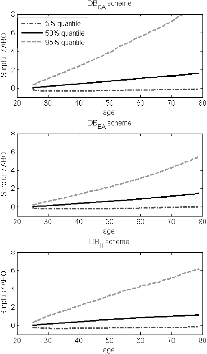
The distributions of the funding status over time are critical for the welfare of the future cohorts and the sustainability of the schemes. Seriously underfunded situations are difficult for the sustainability of the fund, as in these situations future generations may want to step out. Figure 4 shows quantile distributions of the normalized funding surplus, S t/L, of the three optimal collective schemes. Due to the positive equity premium, funding surpluses are more frequent (and larger in size) than funding deficits.
Funding status of the collective schemes
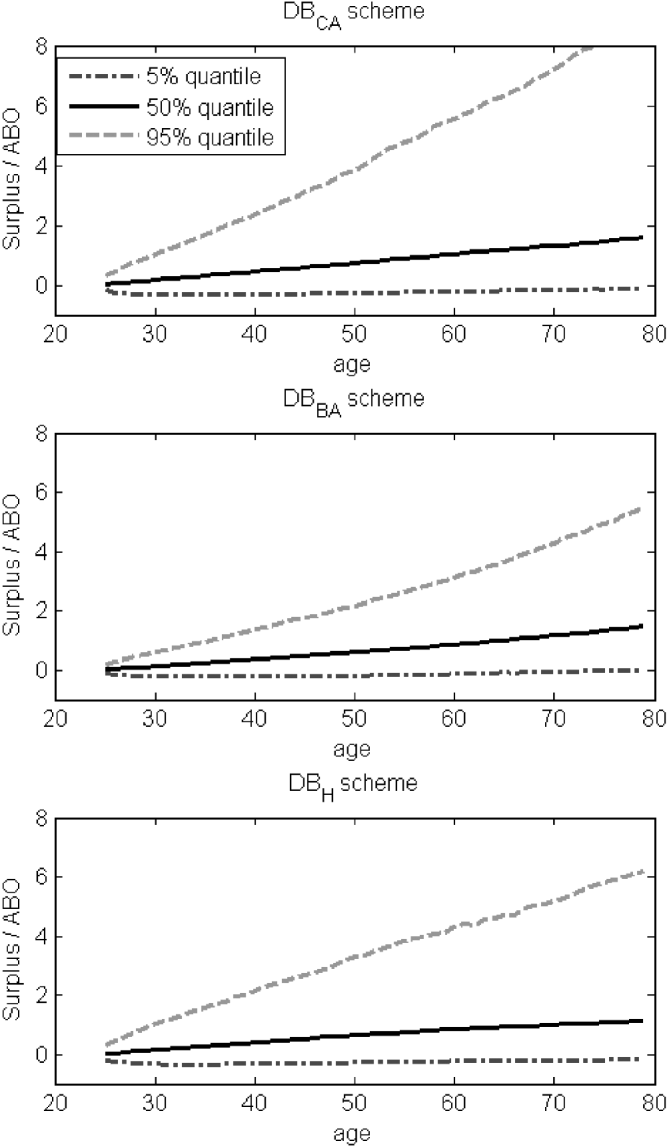
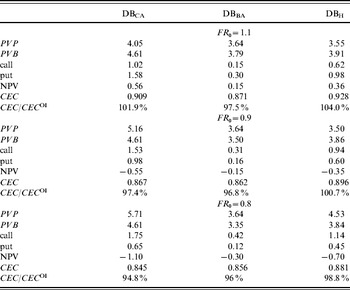
Table 3 shows the welfare gains and losses of entering the initially over- and underfunded schemes (with funding ratios being FR 0=1.1, FR 0=0.9, and FR 0=0.8, respectively). These schemes are set at their optimal design as in Table 1 (middle panel). The new cohort joining an underfunded collective scheme is not necessarily worse off in welfare terms, compared with the optimal individual benchmark. For instance, when FR 0 falls to 0.9 (0.8) initially, the welfare of DBH is 100.7% (98.8%) of that of the optimal individual scheme. Hence, it is possible for well-structured collective pension schemes to absorb funding deficits up to 10% to 20% by intergenerational risk sharing and still enhance the welfare for her participants.
Initially overfunded and underfunded schemes
This table shows the net value transfer (NPV) and the welfare implications of initially over- and under-funded schemes. FR 0 denotes the initial funding ratio. The optimal scheme designs are as shown in Table 1 for γ=5. CEC/CEC OI shows the relative welfare gain or loss to the optimal individual scheme.

Table 3 also shows the market valuation of the intergenerational transfers when the collective schemes are initially underfunded. The net transfers ex ante are non-zero. The net transfers are large and positive, meaning the entry cohort makes up a large part of the initial deficits, by either higher contributions (DBCA, DBH) or lower benefits (DBBA, DBH). Furthermore, the net transfers are proportional to the degree of underfunding. For instance, the value of net transfers doubles when FR 0 is reduced from 0.9 to 0.8. Initially overfunded schemes are also reported in Table 3. The market values of the net transfers starting with FR 0=1.1 are mirror images of FR 0=0.9.
4.3 The impact of having outside savings
In Section 3, in order to optimize the collective pension schemes, we have assumed that participants do not save outside of their pension schemes. However, in reality, people do have the possibility to save and invest outside of pension schemes. In this subsection, we quantify the welfare gain for participants who save and invest both through a collective pension scheme and outside the pension fund in private investment accounts.
We integrate the mandatory contributions and benefits as part of income, which we call disposable income. The normalized disposable income before retirement is 1−p t=1−p−αS t/R, and after retirement it becomes b t=b+βS t/(T−R). The individual takes the disposable income (from DBCA, DBBA, or DBH) as given, and chooses optimally his consumption and portfolio allocation for the wealth outside of the pension scheme (subject to no borrowing and no short-selling constraints). The difference between his disposable income and the optimal consumption is then the additional saving outside of the pension fund. Let W t denote the amount of outside savings, and ωt as the equity weight within the outside saving, then the individual's optimization problem is as follows

and subject to the wealth dynamics



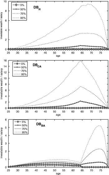
For the default setting, the certainty equivalent consumption (CEC) is reported in Table 4. Our key findings are as follow. First, allowing participants to save outside of the collective pension schemes indeed improves the welfare. However, the welfare improvements are very marginal for the hybrid scheme (0.1% of CEC) and the DBBA scheme (0.2% of CEC). For the DBCA scheme, the welfare improvement is about 1.3%, which is more substantial. Therefore, we conclude that, in schemes with well-organized IRS (e.g. DBH), assuming saving only via pension schemes is not so restrictive, since the added welfare gain of having outside saving is small. Second, when allowing participants to save additionally outside of pension schemes, the DBCA participants may also obtain a higher welfare level (CEC=0.901) than that of the optimal individual (OI) benchmark (CEC OI=0.891). Thirdly, the optimally accumulated outside saving is moderate, confirming that our assumption of no outside saving is not so restrictive. Figure 5 shows the levels of the accumulated outside savings throughout the life cycle. For the optimal hybrid scheme participants, the median of the outside saving reaches its peak level of less than one year salary around age 65. The median levels of the other two collective schemes are also low (at one to two years of salary). In some cases (e.g. the 95% quantile), the outside savings could reach a larger amount, which happen in scenarios with high returns and a high funding surplus. Finally, when outside saving is allowed, individuals often invest their outside savings heavily in equities. Notice that the median of equity weight is at the 100% level in Figure 6.
Wealth accumulation outside of the collective schemes

Portfolio allocation in the outside savings

Collective scheme participant with additional outside savings
The first row is reproduced from Table 1. The second row of the table shows the welfare level (CEC/salary) obtained by collective scheme participants with outside savings, as described in Section 4.3. Compared to the first row allowing outside saving does improve the welfare, as given in the third row.

5 Welfare of future generations
Having shown that IRS in collective pension plans can be welfare improving for the new entry cohort, we investigate in this section whether or not the welfare gain of the new-entry cohort comes at the expense of the future cohorts. To do this, we compute the ex ante the expected welfare of future cohorts with the initial condition that the pension funds are fully funded at t=0. We calculate the certainty equivalent consumption, CECf, of the future cohorts (the future 25-year-old's) who will enter into the pension fund in f years' time, with f=0,1,2,…,1000 years. The expected welfare of cohort f obtained from participating in a given pension scheme, during his life time from year f till f+T, is measured in terms of certainty equivalent consumption as follows

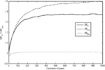
Figure 7 presents the CEC of the future cohorts (up to cohort f=1000) relative to that of the optimal individual scheme, CEC f /CEC OI, which can be seen as the relative welfare gain or loss over the individual benchmark. The expected welfare of all future cohorts is higher than the time 0 entry cohort. The welfare is steadily increasing for future cohorts and converging to a level much above the level for the entry cohort. For instance, the welfare of DBH scheme stabilizes at 130% of that of the OI scheme after 100 years. From this result, we can conclude that the expected welfare gain of the current entry cohort is not at the cost of the future cohorts from an ex ante perspective. Although optimization occurs by the entering generation, the fund is expected to build up a buffer, and is, in expectation, overfunded in the long run. For the DBH scheme, the median size of the surplus becomes twice as large as the size of the liability after 200 years. Due to these transfers, future cohorts are able to benefit from the positive equity premium before they are born. Intergenerational risk sharing together with asset accumulations greatly enhance the intertemporal risk smoothing capability of the economy with collective pension schemes.
Future generations under the generation-0 optimal schemes

An alternative way to design the collective schemes is to take into account the welfare of future generations by taking a social planner's view. Suppose the social planner's objective is to maximize a weighted sum of entry and future cohorts' life time expected utility by optimizing the pension scheme {p,α,β,ω} at time zero

where 0<Δ<1 is the social planner's weighting factor for future cohorts. There is no clear guidance as to how Δ should be chosen. Gollier (Reference Gollier2008) imposes that the assets of the pension fund follow a martingale; this assumption implies Δ=0.937, given his other parameter values. Sleet and Yeltekin (Reference Sleet and Yeltekin2008) argue that the social planner should have discount factors that (weakly) exceed those of agents to make the policy credible. We assume the weighting factor of the social planner is the same as individuals’ subjective discount factor, hence Δ=e −δ=0.96.Footnote 10 We calculate the social planner's designs for individuals with risk aversion of γ=5.
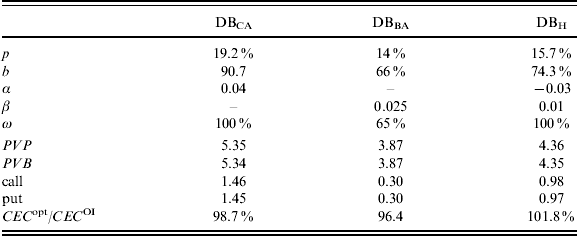
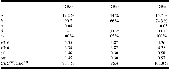
Table 5 shows the results for the social planner's optimal pension schemes. Comparing the socially optimal schemes with the schemes optimized for the f=0 entry cohort in Table 1, we see that the values of α and β are slightly lower and the portfolio choice becomes more risky. These results indicate that shocks in the funding surplus are shared by more generations under the socially optimal schemes. Table 5 also shows the market value of the intergenerational transfers under the socially optimal schemes. Indeed, the market value of transfers (calls and puts) are larger compared with that of Table 2. CEC opt shows the certainty equivalent consumption of the time 0 entry cohort under the scheme optimized by the social planner. From comparing CEC opt with CEC in Table 1, we find that the welfare of the time 0 entry generation is slightly reduced under the social planner's schemes. These results do not materially change for different risk and time preferences or a lower equity premium; the long-run welfare gains for the future cohorts are still substantial.
Socially optimal collective schemes
This table shows the social planner's optimal designs with weighting factor Δ=δ=0.96 and risk aversion γ=5. CEC opt is the certainty equivalent consumption of the time 0 entry cohort under the optimal schemes chosen by the social planner.
6 Conclusion
We have used the institutional setting of funded pension schemes to study welfare aspects of intergenerational risk sharing. Typical for such collective pension plans is that pension benefits and/or pension contributions may depend on the funding status. From the perspective of a newly entering cohort, we optimize the explicit asset allocation and risk-allocation rules, which specify who of the stakeholders, when, and to what extent they take part in risk bearing.
We show that well-designed funded schemes with intergenerational risk sharing are welfare improving over and above the optimal individual scheme by 2–4% in terms of certainty equivalent consumption per year. Efficient risk sharing should involve both retirees and current and future workers. The hybrid defined benefit scheme, where risks are shared between working and retired cohorts, performs better than schemes where risks are only borne by workers or retirees. Secondly, IRS increases the risk-bearing capacity of the economy and hence increases the demand for risky investment. Thirdly, the initially fully funded collective pension schemes with intergenerational risk sharing are a zero-sum game in market value terms; however, they are potentially a positive-sum game in welfare terms. Furthermore, the expected welfare gain of the current entry cohort is not at the cost of the older and future cohorts, from an ex ante perspective.
Other sources of persistent systematic risks and market incompleteness, like labor income uncertainty, longevity risk, inflation risk,Footnote 11 and real interest rate risk might further strengthen the welfare-enhancing potential of intergenerational risk sharing. Since these risks are often non-hedgable in the financial markets, IRS via collective schemes may further complete the market, and hence improve welfare as compared to the optimal individual scheme.
Our findings have important implications for the debate on social security reforms worldwide. Many countries are gradually reducing (or planning to reduce) the PAYG social security and promoting the individual defined contribution saving schemes (see for instance recent discussions of Feldstein, Reference Feldstein2005; Diamond and Orszag, Reference Diamond and Orszag2005). Our results show that the individual scheme is not the optimal funded scheme, even in a frictionless world with rational and sophisticated individuals. Collective funded schemes with well-organized intergenerational risk-sharing mechanisms are better choices from a welfare perspective. Furthermore, related to the impact of current global financial turmoil since 2007 on retirement provisions, our analysis implies that funded pension schemes with IRS could facilitate intertemporal smoothing of systematic risks and limit welfare loss for participants.
Appendix: Solution methods
A.1 Optimal individual scheme
This appendix explains the solution procedure solving the optimal individual (OI) consumption and portfolio choice described in Section 2.2. We first rewrite the optimization problem (5)–(8) in discrete time form (at annual frequency), and rewrite the original objective function in the recursive form as follows



where  and R f=exp(r).
The problem is solved using the dynamic programming principle, solving backwards from the last to the first period. For the final period, the optimal consumption c T*=W T, and the functional form of indirect utility is known, as  . Then, we proceed backward in time to t=T−1.
The procedure for T−1 starts by defining a new variable a t=W t−c t, as the after-consumption wealth. Following Carroll (Reference Carroll2006), we construct a grid of  . Now we solve for the optimal consumption and portfolio policies for each given a j. The first order conditions with respect to ωt and c t are


The envelope theorem implies that u′ (c t)=U′ (W t), since

Replace U′(Wt+1) by u′(c t+1) in the two first-order conditions, we have


where  denotes the optimal consumption policy at time t+1, and I u(·) denotes the inverse function of u′(c t). Using any numerical solver, equation (28) will give the optimal portfolio weight ωt*(a t) for any given amount of investment a t. Because of the borrowing and short-selling constraints, we then impose the restriction 0 ⩽ωt*⩽1. Then, equation (29) gives the corresponding consumption c t*(a t) for any given amount of investment a t. Finally, the optimal wealth process is endogenously determined by
 . The advantage of this method is that the numerical search is only needed once in solving ωt*(a t), while c t*(a t) can be directly obtained from equation (29).
Following the same procedure illustrated above, we can solve the model backward in time to t=1. To generate the average pattern of life cycle portfolio holding, we simulate the model from time 1 to T for 10,000 scenarios, and take the average over all simulated scenarios.
A.2 Collective schemes
The optimization problem of collective schemes, equation (17), is a static problem, since all the decision parameters {p,α,β,ω} are constants. The collective schemes are solved using Monte Carlo simulations and grid search. We first construct a four-dimensional grid for the decision parameters. For each combination of the parameters, we simulate the wealth dynamics (11) at each point in time, evaluate the resulting funding surplus and determine the state contingent contributions and benefits p t and b t according to the risk-sharing rules in equations (15)–(16). When p t and b t are determined, we evaluate the objective function (17) for the new entry cohort. A numerical grid search identifies the global maximum of the welfare function (17) and its corresponding parameter values {p,α,β,ω}.