The nineteenth-century British economy is often described in terms of a North-South divide. Regional specialization is usually explained in terms of endowments of coal and its attraction to the Victorian staple industries for which it was an important input because of steam power.1
See, for example, Langton and Morris, “Introduction”; Lee, Regional Economic Growth; and Pollard, Peaceful Conquest.
von Tunzelmann, “Coal.”
Gourvish, Railways, p. 31.
Hudson, “Regional Perspective.”
At some point late in the nineteenth or early in the twentieth century a different rationale for industrial location started to emerge. Once electricity became available as an alternative source of power, industry had more freedom to move away from coalfields, and increasingly complex products and mass production techniques came to the fore.5
Lee, Regional Economic Growth.
Dennison, Location of Industry; and Hume and Oglethorpe, “Engineering.”
For the former see Venables, “Equilibrium Locations”; and for the latter, Richardson and Smith, “Sectoral Growth.”
The descriptions in the British historiography are informal both in the sense that they are not grounded in economic theory nor have they been formulated as testable hypotheses and subjected to quantitative scrutiny. This is in sharp contrast with the economic history of American industrialization.8
Kim, “Economic Integration” and “Regions.”
The New Economic Geography has formalized a number of propositions regarding the pull of centrality that are of interest in this context. At bottom, these can be summarized as predictions that when transport costs are very high or very low, economic activity will be spatially dispersed, but when transport costs enter an intermediate zone, firms' location decisions involve consideration of market access as well as production costs. When transport costs are “intermediate,” it may be advantageous to locate near to industrial customers, and suppliers and increasing-returns industries may also prefer to locate their (large) plants at central locations.9
Venables, “Equilibrium Locations.”
Thus, at some point, falling transport costs supplement the factor endowment arguments with a market access explanation of industrial location. This could happen in the context of improvements to an existing transport technology rather than awaiting the introduction of a new mode. So, although the increasing attraction of central locations and the diminishing appeal of outer Britain has often been linked to the arrival of motorized road haulage, continuing reductions in the cost of rail freight and coastal shipping may eventually have had similar implications. Regional market potential is fundamental to the pull of centrality, and this was increasing at a varying pace across British regions as World War I approached and both regional incomes and also the proximity of foreign markets were exposed to globalization.10
Crafts, “Market Potential.” For the definition of market potential and some estimates, see below.
Looking at the economy through this lens might have ramifications for the measurement of economic benefits from transport improvements. Gary Hawke, who estimated the social savings of railways, explicitly recognized this as follows: “If as a result of the establishment of railways, a particular industry became more concentrated geographically, and if this resulted in a lowering of the real costs of that industry, then the establishment of the railways has given the economy the equivalent of extra resources. The railways have then contributed to economic growth in a way that is not reflected in the social saving.”11
Hawke, Railways, p. 382.
Venables and Gasiorek, “Welfare Implications.”
Ibid., pp. 392–95.
An alternative way to estimate the contribution of a new technology to economic growth would be to use growth accounting techniques. In that context, the cost reductions that flowed from induced decreases in the real costs of transport-using industries would be reckoned as spillover effects on total factor productivity (TFP) growth. Nicholas Crafts recently examined the impact of steam (including both railways and steamships as well as stationary steam engines) on British economic growth using a methodology of this kind.14
Crafts, “Steam.”
In the light of this discussion, in the rest of the article we provide a description and econometric analysis based on a reduced form equation derived from a general equilibrium model of the location of industrial employment at the two-digit level for Britain in the decades from the railway age to World War I. This is used to address the following questions: What happened to the location of industry over time? What happened to market potential as globalization impinged on the economy? Is there evidence that the location of industry responded to the pull of centrality as transport costs fell? What implications are there for measurement of the contribution of steam-based transport to economic growth?
REGIONAL SPECIALIZATION
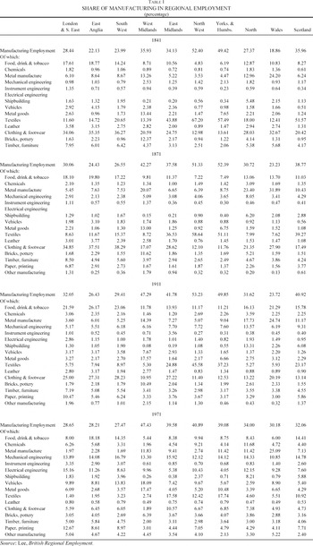
How did regional specialization evolve in the period 1841 to 1911 and how different was this experience from that of the post-1945 economy whose freight transport was dominated by road haulage rather than railways and coastal shipping? The context for this enquiry is set out in Table 1, which shows the extent to which the share of manufacturing in total employment differed across regions and provides a breakdown of the sectoral composition of employment within manufacturing. The table shows that the British economy was still industrializing through 1911, at which point the highest shares of manufacturing were in the North West, West Midlands, and Yorkshire and Humberside whereas the south, with the exception of London, was much less industrial. By 1971, this “North-South divide” was still clearly visible but much less pronounced. A notable feature of the pre-1911 economy was the tendency for a high fraction of manufacturing in a region to be in one sector; there are 13 instances of a sector comprising more than 20 percent of manufacturing employment before 1911 compared with only one in 1971.

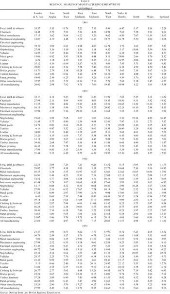
Regional shares of employment in the total for each industry (which in logarithmic form will be the dependent variable for our econometric analysis) are set out in Table 2. The overall picture is of quite modest changes but one or two relatively large shifts stand out. For example, chemicals moved steadily to North West, shipbuilding gravitated to the North and Scotland and away from South East and South West, vehicles expanded markedly in West Midlands but contracted in the southern regions. Textiles became even more concentrated in North West but declined in Scotland.

For several sectors, particular regions have persistently high location quotients including shipbuilding in North, metal manufacture in Wales, and metal goods in West Midlands.15
The location quotient is defined as sik/sallk, in other words, it compares the share of the region in employment in the ith industry with its share in manufacturing employment as a whole.
Lee, Regional Economic Growth, p. 121.
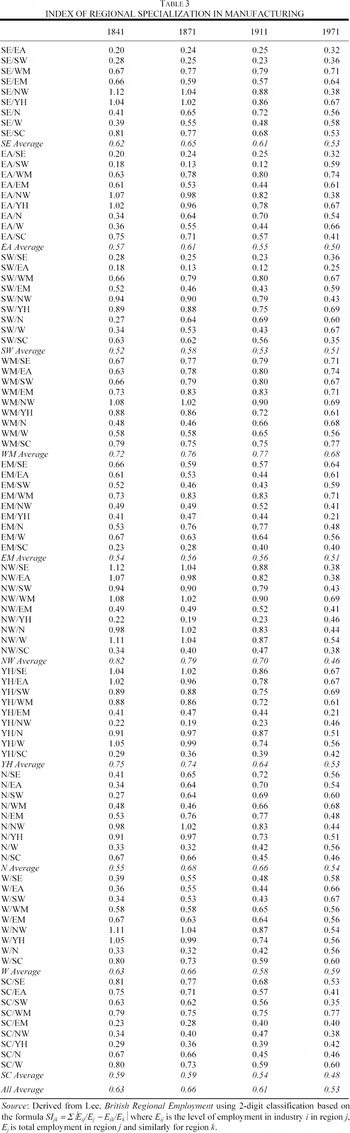
Table 3 reports Paul Krugman's index of regional specialization for each pair of regions.17
Krugman, Geography.
Kim, “Expansion of Markets,” table 1.

From 1841 to 1911 the South East, East Anglia, and South West were quite similar to each other and very different from North West, West Midlands, and Yorkshire and Humberside, again reflecting a “North-South divide.” By 1971 these southern regions were somewhat less similar to each other and much less different from North West, in which textiles were now less prominent. By 1971 the average value of the specialization index had fallen to 0.53.
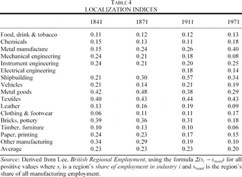
Table 4 reports the coefficient of localization of each industry. This differs quite considerably. Textiles were always relatively localized. The biggest increase in spatial concentration between 1841 and 1911 was in shipbuilding. On the other hand, food, drink and tobacco, leather, clothing and footwear, and timber and furniture remained dispersed throughout. Through 1911 the average coefficient of localization remained unchanged but from then to 1971 it exhibited a modest decrease.

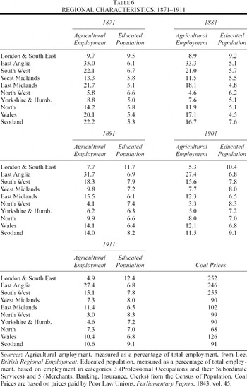
The underlying reasons for regional specialization are to be found in the characteristics of industries and regions and in the interactions of these characteristics. Accordingly, Tables 5 and 6 set out values of the individual variables, which will be used later in our econometric work. Table 5 displays data on industrial characteristics including size of plant, and the intensities of use of white-collar workers and of steam power. It also reports on linkages to other industries in terms of extent of intermediate input use and of sales to industrial users. With regard to industrial characteristics, we are reliant on the 1907 Census of Production and the input-output table for that year constructed by Mark Thomas.19
Thomas, “Input-Output Approach.” Clearly, it is not ideal to assume that the input-output relationships remained unchanged throughout the period 1871–1911. We therefore undertook a robustness check on our results using preliminary estimates from an input-output table for 1851, prepared by Charles Feinstein. In essence, all our econometric results reported below remained intact when these alternative data were used. We are very grateful to Charles Feinstein for sharing his estimates with us and letting us have the opportunity to make this test.

There was quite substantial variation of these characteristics across industries. For example, Table 5 shows that chemicals were intensive in the use of educated workers but textiles were not. Plant size was large in shipbuilding and textiles, which had high localization coefficients, but small in food, drink & tobacco, leather, and timber and furniture, which were spatially dispersed. The sectors with the biggest linkage effects were bricks and pottery and metal manufactures, which were also the most steam-intensive industries.
Table 6 provides data on regional characteristics including education of the population, agricultural employment, and coal prices. As might be expected, East Anglia had the highest proportion of agricultural employment. From Table 2 it is apparent that it also had relatively high location quotients in food, drink and tobacco, and in leather, which were the two sectors most intensive in the use of agricultural inputs. London & South East has a much higher proportion of educated workers than any other region. The industries that used white-collar labor most intensively (chemicals, food, drink and tobacco, and instrument engineering) all have high location quotients in that region. Coal abundance was a feature of northern but not of southern regions.20
We measure coal abundance in terms of relative prices prevailing before the railway age, which gives a clear indication of the traditional areas distinguished in standard accounts of nineteenth-century industrial location.

THE EVOLUTION OF MARKET POTENTIAL
As has been explained, the notion of market potential is important for explanations of industrial location decisions based on New Economic Geography. Market potential varies across locations because of transport costs. To estimate market potential we follow the approach of David Keeble and his collaborators but modify the details to match the circumstances of an earlier transport era.21
Keeble et al., “Regional Accessibility.”
We have followed the standard convention of approximating “self-distance” by using the formula dii = √(area of region/π) which gives a distance value one-third of the radius of a circle of the same area as region i; see Keeble et al., “Regional Accessibility.”
These estimates were derived from Prados de la Escocura, “International Comparisons.”
The major problems in estimating market potential for this period lie in obtaining estimates of regional GDP for British regions and in the details of the distance deflation procedure.24
For an alternative method that can be used to compare early- and late-twentieth-century market potential, see Crafts, “Market Potential.”
Geary and Stark, “Examining Ireland's Post-Famine Economic Growth”; full details of the construction of the estimates can be found in Crafts, “Regional GDP.”
Armstrong, “Role of Coastal Shipping,” estimates that coastal shipping accounted for 59 percent of internal freight ton-miles in 1910. Road haulage was negligible until after the First World War.
Kaukiainen, “How the Price of Distance.”
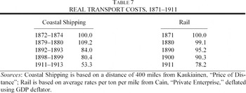
Changes in market potential over time can result from either or both of a shift in the spatial distribution of GDP or in relative transport costs. In the period 1871–1911 developments in steamship technology and continuing improvement of railway productivity drove transport costs sharply down. However, as Table 7 reports, after about 1880 costs of sea transport fell by more than those of rail freight. The broad implication of this is that market potential rose relatively more in regions with good access to the sea, such as Scotland, compared with landlocked regions, such as the Midlands.

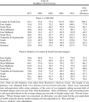
Table 8 reports estimates for regional market potential for the census years 1871 to 1911. In all cases, market potential was increasing appreciably at a time of economic growth at home and abroad. From the point of view of location decisions, it is relative market potential that matters. Interestingly, the location quotients for the sectors with the largest linkages (bricks and pottery and metal manufactures) in the regions with the largest market potential (London and the South East and North West) are all well below one.
There was an obvious change in relative market potential over time in that the Midlands lost ground and London & South East gained with the result that East Midlands and West Midlands, respectively, fell from 65.0 to 55.9 percent and from 69.1 to 59.7 percent of market potential in London & South East between 1871 and 1911. However, it should also be noted that Outer Britain (North, Scotland, and Wales) also improved its position. For example, Scotland's market potential rose from 67.5 to 79.3 percent of that in London & South East between 1871 and 1911. The final column of Table 8 removes the effects of changes in relative transport costs by recalculating 1911 market potential using the rail-equivalent distances of 1871.28
Thus sea miles are converted into rail miles using the 1871 relative transport costs, and an 1871 rail mile is taken to be 1/0.782 of a 1911 rail mile. In terms of the exercise subsequently undertaken in Table 11, this scaling factor has no effect, it is only the change in relative costs that matters.

MODELING THE LOCATION OF INDUSTRY
In order to analyze regional specialization it is appropriate to employ location theory. There are two obvious possibilities, namely a Heckscher-Ohlin type factor endowment hypothesis or a New Economic Geography market access hypothesis. They both rely on the interaction of regional characteristics with industrial characteristics. The rationale for the emphasis on these interactions lies in the general equilibrium nature of the system. Thus, Heckscher-Ohlin theory predicts that industries that use a factor of production intensively will tend to locate in regions which are abundantly endowed with that factor whereas New Economic Geography theories predict that the attraction of a region's market potential is greater the more an industry sells to or buys inputs from other industries. These theories should probably be regarded as complementary rather than mutually exclusive, and our empirical analysis will therefore be based on a model recently proposed by Karen Midelfart-Knarvik et al., which encompasses them both.29
Midelfart-Knarvik et al., “Location.”
In this model, regions are heterogeneous in various characteristics such as endowments of natural resources and proximity to markets. Similarly, industries differ in their various attributes such as the intensity of use of production factors such as natural resources and skilled labor, and their reliance on intermediate inputs. In equilibrium, all industries cannot be in the same place, but we expect that industries that value a regional characteristic most highly will succeed in locating there. So, for example, we might predict that if cheap coal matters for location, industries that use steam power intensively will gravitate to coal-abundant regions. The interaction between the industrial characteristic, steam power use, and the regional characteristic, coal abundance, is what attracts the industry to the region. If, on the other hand, cheap coal does not matter to industry, then coal abundance should have no attraction for any industry.
The Midelfart-Knarvik et al. model can be written as a reduced-form equation to explain a dependent variable that is the share of each region in total British employment in each industry. The independent variables are controls for size, regional characteristics, industrial characteristics, and interactions between these regional and industrial characteristics. In our implementation of the model, we consider the following six interactions: educated population availability and white-collar worker intensity, coal abundance and steam power use, share of agricultural employment and agricultural input use, market potential and plant size, market potential and sales to industry, and market potential and intermediate input use. The first three of these interactions are predicted by the Heckscher-Ohlin theory based on factor endowments; the last three are predicted by New Economic Geography to be activated when transport costs are at the right “intermediate” level such that the pull of centrality kicks in. The model permits evaluation of the relative importance of these various interactions.
The first market-potential interaction hypothesizes that industries operating at relatively large scale will value highly locations relatively close to market demand, which may be true at some but presumably not at all levels of transport costs. The second market-potential interaction based on backward linkages supposes that industries which sell relatively large fractions of their output to other firms rather than final consumers tend to prefer locations relatively close to other producers. The third market-potential interaction predicts that industries which use relatively large amounts of intermediate goods will prefer locations of high market potential. Here the importance of forward linkages is the key but, again, how strongly firms value centrality is likely to depend on transport costs; cheaper inputs have to be traded off against a higher cost of sending goods to final consumers.
Formally, the basic model can be written as follows

where sik is the share of industry k in region i, popi is the share of British population in region i, and mani is the share of British manufacturing employment in region i; y[j]i is the level of the jth regional characteristic in region i; x[j]k is the industry k value of the industry characteristic paired with regional characteristic j. Thus, the interaction forces are represented by the terms in the summation. Finally, α, ϕ, β[j], γ[j] and χ[j] are coefficients to be estimated.
To understand this specification, it is easiest to consider one particular characteristic, say j = skilled labor. So x[skilled labor]k is white-collar worker intensity of industry k and y[skilled labor]i is educated-population abundance of region i. The following interpretation can then be given to the model: First, there exists an industry with a level of skilled-labor intensity χ[skilled labor] such that its location is independent of regional skilled-labor abundance. Second, there exists a level of skilled-labor abundance γ[skilled labor] such that the region's share of any industry is independent of the skilled-labor intensity of the industry. Third, if β[skilled labor] > 0, then industries with skilled-labor intensity greater than χ[skilled labor] will be induced to locate near regions with skilled-labor abundance greater than γ[skilled labor]. Estimation of the model will produce the following key parameters for each interaction variable: γ[j], χ[j] and β[j] with j running over the six interactions. If, for example, skilled labor is an important determinant of location patterns, we should see a high value of β[skilled labor].
Expanding the relationships in the above equation we obtain the estimating equation,

This gives a list of independent variables that comprises scaling terms, regional characteristics, industrial characteristics, and interactions between regional and industrial characteristics, as in Table 9. The coefficients of the two size variables, α and ϕ, are straightforward, and c is a constant term. The estimated coefficients of the regional characteristics, y[j] and the industry characteristics, x[j] are estimates of −β[j]χ[j] and −β[j]γ[j], respectively, and so are expected to have negative signs.

The estimated coefficients of the interaction variables, y[j]x[j] are estimates of β[j], which are expected to be positive. This is the crucial set of parameters in the model. The relative magnitude and statistical significance of this coefficient on, for example, educated population × white-collar workers provides us with a measure of how important this factor endowment was in influencing the location of industries in pre–World War I Britain.
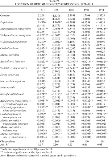
For each census year from 1871 to 1911 this equation is estimated by OLS, pooling across industries. The results are reported in Table 9. The intercept is followed by the two terms which pick up regional size effects, then the coefficients of the four regional characteristics, y[j], the six industry characteristics, x[j], and finally the six interaction variables, β[j]. The coefficients of interest are those on the interaction variables, which capture the joint role of regional and industrial characteristics in the location of industry. Transport costs play a role only if the market potential interactions are a significant determinant of industrial location. If falling transport costs were making market potential considerations matter more, then we should see market potential interactions becoming significant as time goes on.
Of the two size variables, manufacturing employment always has the right sign and is generally quite close to unity. In almost all cases, the coefficients of the regional characteristics have the expected negative signs but are usually statistically insignificant. With respect to the industry characteristics, the coefficients of the variables share of agricultural employment, educated population, and size of establishment have the expected negative signs and are significantly different from zero throughout.
Turning to the key interaction variables, the coefficients relating to interactions involving factor endowments have the correct (positive) signs; educated population × white-collar workers, coal abundance × steam power, and agricultural employment × agricultural input use are significant virtually throughout. This confirms the importance of factor endowment variables in the location of industry. The significance of coal endowments familiar from the traditional literature is also confirmed, but other aspects of factor endowments seem also to have mattered, namely, human capital and land. Moreover, some caution is probably appropriate before these results are taken to be an endorsement of a straightforward Heckscher-Ohlin model of industrial location. For example, proximity to coal may have affected the choice of location of industries such as cotton textiles early in the nineteenth century but later on they may have been anchored in coal-abundant areas by Marshallian external economies of scale.
With respect to the coefficients of the interaction variables involving market potential, market potential × size of establishment has the expected positive sign and is statistically significant but the coefficient decreases over time. This indicates that the pull of centrality for increasing-returns industries was weakening over time as transport costs fell. Market potential × intermediate input use and market potential × industry sale generally have the wrong sign but are always insignificant. Thus, there is no evidence that market potential mattered for location decisions either through upstream or downstream linkage effects even in 1911. This may indicate that transport costs were still too high for these considerations to have an impact on industrial location.30
Strictly speaking, these results could imply that they may already have been too low but given the finding by Midelfart-Knarvik et al., “Location,” pp. 36–37, that these effects started to have an impact in Europe only in the 1990s, we prefer the interpretation in the text.
Lee, Regional Economic Growth, p. 204.
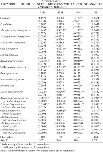
It is possible that our coefficient estimates may suffer from biases caused by potential endogeneity problems, in other words, some of the explanatory variables such as manufacturing employment are determined in the model. Ideally, such problems would call for instrumental variable estimation, but there seems to be no way to implement such an approach. As a crude alternative we have experimented with a regression on lagged values of the regional variables that are time-varying. As can be seen from Appendix Table 1, there is no material change in the estimation results.
A glance back at Table 5 helps to make sense of these results. As was noted earlier, the sectors with the biggest linkage effects (bricks, metal manufactures, and leather) were not among the biggest movers in Table 2. The first two of these industries were the most intensive in the use of steam, and leather was the most intensive user of agricultural inputs. In each case, there was a strong factor-endowment reason for their location, which, in a general equilibrium context, dominated the attraction of market potential. These industries do indeed seem to epitomize the traditional argument that proximity to natural resources was crucial in nineteenth-century location decisions and this seems to have prevailed all the way through to World War I.32
We have explored alternative econometric specifications to estimate our data set by pooling the five sets of cross-section data. Two sets of estimators that we considered are: the pooled least square estimator that represents the average of the within-groups and between-groups estimators; and least square estimators with region or sector specific effects or period specific effects that represent within-group estimators. Each of these leaves the regression results fairly intact. All these results of alternative specifications are available from the authors upon request.
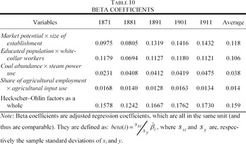
Table 10 considers the overall proportion of the variance explained by the various statistically significant interaction variables. This provides two important qualifications to the traditional account of industrial location being heavily influenced by natural resources. First, the most important factor-endowment interaction is seen to be that of educated population × white-collar workers. This suggests that the role of human capital in nineteenth-century British industrial location has been underestimated. Second, the single most important interaction variable is market potential × establishment size, although this contributes less than the sum of the three factor-endowment interactions. In sum, Table 10 suggests that there has been a tendency to oversimplification in discussions of the geography of British industry.

GROWTH EFFECTS OF STEAM—POWERED TRANSPORT
In previous sections we have shown that the pattern of localization and specialization of British industry changed relatively little in the decades before World War I. We have also found that the most important determinants of industrial location decisions were based on the interaction of regional factor endowments and industrial factor intensities. New Economic Geography forces appear to have been relatively weak in that there was no role for the pull of centrality through linkage effects. There was, however, a role for market potential through the attraction that it offered to industries with large plant size. Accordingly, it is important to ask whether the impact of falls in steam-powered transport costs on market potential would have had much impact on regional shares of manufacturing employment according to these regression estimates. To do this, location of industry as predicted by a regression using actual market potential in 1911 can be compared with the predictions of a regression based on counterfactual market potential in 1911 based on 1871 distances, as reported in Table 8.
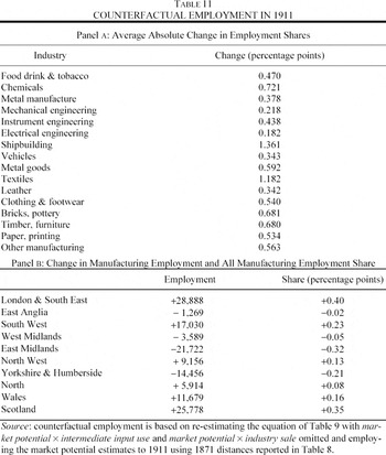
Table 11 is based on results obtained by re-estimating the equation omitting the insignificant market potential interaction variables and replacing the actual 1911 market potential variable with the value that would have been observed if transport costs had remained as in 1871 and then comparing the predictions for the dependent variable with those obtained using the original values for market potential on the right-hand side. The general impression that emerges from this exercise is that the impact of transport costs improvements on the location working through the remaining interaction of market potential and size of establishment is quite modest.

Looking at panel A of the table, one can see that the overall average change in a region's employment share of an industry is a little under 0.6 percentage points and that inserting the counterfactual market potential with the transport costs change neutralized does not have much effect on the large shifts in employment shares highlighted earlier. Thus the North West's share of textiles and chemicals rose by 5.65 and 4.32 percentage points, respectively, but the changes in the predicted shares are only 0.30 and 0.24 percentage points. Similarly, shipbuilding in the North and Scotland gained 8.94 and 6.33 percentage points, respectively, but the changes in the predicted share are only 1.13 and 0.99 percentage points.
Turning to the impact of the counterfactual market potential on regions, the total changes in employment are on average about 2.4 percent of regional employment and in no case is the change as much as 5 percent. Table 2 shows that the biggest gain in regional share of all manufacturing employment between 1871 and 1911 is 2.37 percentage points in London & South East but the change in predicted share from inserting the counterfactual market potential variable is only 0.40 percentage points. So, although improvements in steam technology reduced the costs of both water and railway transport quite appreciably between 1871 and 1911, as Table 7 reported, the impact that transport cost reductions had through the interaction of market potential and size of establishment was small—only very marginal shifts in industrial location can be attributed to this variable, according to Table 11.
In the light of these results, it seems reasonable to argue that there is no reason to believe that estimates of the social savings from railway freight transport need to be revised on account of New Economic Geography-type externalities in the transport-using industries. Nor is there any strong case to argue that steam-powered transport improvements generated substantial TFP spillovers to add to their contribution to growth in the later decades of the nineteenth century. The dramatic relocations of industry that are such a striking feature of Alfred Chandler's account of the rise of mass production and mass distribution as railroads integrated the American domestic market are notable by their absence. So traditional neoclassical approaches to measuring the contribution of better transport to British economic growth are perfectly adequate.33
Chandler, Visible Hand.
CONCLUSIONS
Our findings can be summarized in terms of answers to the four questions that we posed in the introduction.
First, the overriding impression is that patterns of the location of industry exhibited marked persistence. This is supported by the summary indices of localization and specialization that were reported in Tables 3 and 4, although, as Table 1 shows, there were changes in regional employment shares. In line with the traditional literature, our regression results suggest that factor endowments were the most important influence on the location of industry and that this acted to anchor activities that were intensive in the use of natural resources, especially coal, in their existing locations. At the same time, the factor endowment hypothesis should not be oversimplified and human capital, in which London & South East was relatively well endowed, was also an important influence on industrial location.
Second, market potential was affected by the changes in transport costs that were driving globalization forward in the period. In particular, sea transport costs fell relative to those of rail transport and GDP in important markets overseas, such as the United States, increased faster than in the United Kingdom. The implication of this was that market potential in London & South East and in the regions of Outer Britain (North, Scotland, Wales) grew faster than in the Midlands, as was reported in Table 8. Thus, market potential in West Midlands fell from 69.1 percent to 59.7 percent of that in London & South East between 1871 and 1911, whereas over the same period in Scotland it rose from 67.5 percent to 79.3 percent of the London & South East level.
Third, the regressions in Table 9 provide evidence that the pull of centrality affected industrial location decisions through its attraction for industries with relatively large size of establishment. However, as transport costs fell over time the force of this attraction was weakening and industries seem to have become freer to locate on the basis of production rather than distribution costs. There is no evidence that market potential influenced location decisions through linkage effects. This probably reflects both the stronger pull of natural resource considerations and that, in this pre-road-haulage era, transport costs were still too high for these effects to materialize.
Fourth, Table 11 indicates that falling transport costs had only weak effects on the location of industry in the period 1871 to 1911. This means that existing calculations of the impact of steam-powered transport on British economic growth probably do not need to be revised on account of productivity spillover effects.
Appendix
The following table displays the results of re-estimating the regressions using ten-year lagged values of the regional characteristics.

Financial support from the Economic and Social Research Council under Grant R000239536 is gratefully acknowledged. We would like to thank Steve Redding, the editor, and an anonymous referee for helpful comments on an earlier version of this article. Any remaining errors are ours.