1 Introduction
Directed motion of colloidal particles via self-created gradients or fields has become an area of significant scientific interest and potential. Drug or gene delivery (Coti et al. Reference Coti, Belowich, Liong, Ambrogio, Lau, Khatib, Zink, Khashab and Stoddart2009; Kagan et al. Reference Kagan, Laocharoensuk, Zimmerman, Clawson, Balasubramanian, Kang, Bishop, Sattayasamitsathit, Zhang and Wang2010; Gao et al. Reference Gao, Kagan, Pak, Clawson, Campuzano, Chuluun-Erdene, Shipton, Fullerton, Zhang and Lauga2012), neutralizing pollutants (Gao & Wang Reference Gao and Wang2014; Li et al. Reference Li, Singh, Sattayasamitsathit, Orozco, Kaufmann, Dong, Gao, Jurado-Sanchez, Fedorak and Wang2014), directed transport of chemical reagents (Sundararajan et al. Reference Sundararajan, Lammert, Zudans, Crespi and Sen2008; Wang Reference Wang2012) and mixing enhancement (Orozco et al. Reference Orozco, Jurado-Sánchez, Wagner, Gao, Vazquez-Duhalt, Sattayasamitsathit, Galarnyk, Cortés, Saintillan and Wang2014) can be mentioned here. With recent developments in the collective behaviour of self-propelling particles (Theurkauff et al. Reference Theurkauff, Cottin-Bizonne, Palacci, Ybert and Bocquet2012; Buttinoni et al. Reference Buttinoni, Bialké, Kümmel, Löwen, Bechinger and Speck2013; Palacci et al. Reference Palacci, Sacanna, Steinberg, Pine and Chaikin2013), the interest has shifted towards creating active soft materials that, in addition to operating autonomously, also have the ability to sense their surroundings and process this information into smart decisions.
After a decade, it is now well understood that an asymmetric surface chemical reaction on a colloidal particle is able to produce autonomous motions. This observation has been studied both experimentally (Paxton et al. Reference Paxton, Kistler, Olmeda, Sen, St. Angelo, Cao, Mallouk, Lammert and Crespi2004, Reference Paxton, Baker, Kline, Wang, Mallouk and Sen2006; Howse et al. Reference Howse, Jones, Ryan, Gough, Vafabakhsh and Golestanian2007) and theoretically (Golestanian, Liverpool & Ajdari Reference Golestanian, Liverpool and Ajdari2007; Córdova-Figueroa & Brady Reference Córdova-Figueroa and Brady2008; Moran, Wheat & Posner Reference Moran, Wheat and Posner2010; Moran & Posner Reference Moran and Posner2011). In the particular case of non-electrolyte solutions, Golestanian et al. (Reference Golestanian, Liverpool and Ajdari2007), Howse et al. (Reference Howse, Jones, Ryan, Gough, Vafabakhsh and Golestanian2007) utilized a continuum description based on diffusiophoresis (Anderson & Prieve Reference Anderson and Prieve1984; Anderson Reference Anderson1989) to study the locomotion of spherical Janus particles due to a surface chemical reaction. In this case, a chemical reaction takes place on a portion of the particle surface and produces a non-uniform distribution of the product and reactant solutes which in turn induces a diffusiophoretic motion. A similar idea was applied for a thermophoretically self-propelled Janus particle, which consumes an imposed laser energy on half of its surface, thus creating a non-uniform temperature field (Jiang, Yoshinaga & Sano Reference Jiang, Yoshinaga and Sano2010). In contrast, Córdova-Figueroa & Brady (Reference Córdova-Figueroa and Brady2008), Brady (Reference Brady2011) and Córdova-Figueroa, Brady & Shklyaev (Reference Córdova-Figueroa, Brady and Shklyaev2013) applied a colloidal perspective to the problem of catalytically driven self-propulsion, in which a catalytic motor (or motors) does not have to be assumed to be large in comparison with the product (or reactant) solutes and the restriction for diluteness of solutes can be relaxed. Therefore, the results obtained within this approach can be applied to other microscopic objects, such as proteins or even large molecules.
Current efforts in the study of catalytic motors include exploiting propulsion mechanisms and finding alternatives to guide their direction (Sanchez et al. Reference Sanchez, Solovev, Schulze and Schmidt2011; Mozaffari et al. Reference Mozaffari, Sharifi-Mood, Koplik and Maldarelli2016). Moreover, self-propulsion was found even for a symmetric chemical reaction (Popescu, Tasinkevych & Dietrich Reference Popescu, Tasinkevych and Dietrich2011; Michelin, Lauga & Bartolo Reference Michelin, Lauga and Bartolo2013) within a chemotaxis problem (Grima Reference Grima2005; Sengupta, van Teeffelen & Löwen Reference Sengupta, van Teeffelen and Löwen2009). There, self-propulsion emerges as a result of the instability of a stationary state; its direction is determined by an initial perturbation in the solute concentration gradient. For example, the presence of a chemically passive particle (or cargo) connected to a catalytic one causes self-propulsion (Thakur & Kapral Reference Thakur and Kapral2010; Popescu et al. Reference Popescu, Tasinkevych and Dietrich2011; Sharifi-Mood Reference Sharifi-Mood2013; Reigh & Kapral Reference Reigh and Kapral2015). This model provides a good representation of a cargo particle transported by the catalytic motor, a problem of crucial importance for a large number of applications. On a similar note, Shklyaev, Brady & Córdova-Figueroa (Reference Shklyaev, Brady and Córdova-Figueroa2014) and Michelin & Lauga (Reference Michelin and Lauga2015) reported that self-propulsion of a particle with a uniform distribution of a surface reaction arises due to non-sphericity of the particle shape. A direct significance of this study is the realization that even for particles with uniform surface catalytic activity, a change to the surrounding distribution of reagents (or solutes) can occur which, consequently, creates perturbations (or concentration gradients) that directly affect particle diffusivity and the interaction force between nearby particles.
An increasing number of experiments on catalytically driven (active) colloidal particles have shown that the interaction of chemically active particles is more complicated than usual interaction of two non-reactive (passive) particles. Indeed, each chemically active particle changes the distribution of product (or reactant) solutes which, in turn, alters the motion of the other particles. In this case, the motions of active particles are influenced not only by hydrodynamic interactions but also via diffusive interactions of the solute distribution generated (or consumed) on the surface of the active areas of each colloid with the boundary of other colloids. Such is the case in the problem of multicomponent diffusion where a gradient in the concentration of one species can drive the flux of another (Batchelor Reference Batchelor1983; Bird, Stewart & Lightfoot Reference Bird, Stewart and Lightfoot2006). Similarly, depletion flocculation occurs because small particles or molecules (e.g. polymers) are excluded from a zone separating two nearly touching colloidal particles and the imbalanced osmotic pressure of the small particles causes an entropic attractive force leading to flocculation (Asakura & Oosawa Reference Asakura and Oosawa1954; Jenkins & Snowden Reference Jenkins and Snowden1996). Depleted regions between two or more catalytically active colloids can unite and hinder or stop their autonomous motion.
Also, it has been reported recently that active suspensions exhibit perplexing collective behaviour such as swarming, predator–prey interactions and chemotaxis which are reminiscent of biological microorganisms (Hong et al. Reference Hong, Blackman, Kopp, Sen and Velegol2007; Ibele, Mallouk & Sen Reference Ibele, Mallouk and Sen2009; Aranson Reference Aranson2013; Bialké, Speck & Löwen Reference Bialké, Speck and Löwen2015). Active catalytic microswimmers have been experimentally observed to form clusters (Hong et al. Reference Hong, Blackman, Kopp, Sen and Velegol2007; Theurkauff et al. Reference Theurkauff, Cottin-Bizonne, Palacci, Ybert and Bocquet2012) which are ‘live’, i.e. the particles join and leave the clusters frequently. Moreover, the experimental evidence indicates in addition to the large clusters, there are coexistent gas phases where the particles swim freely. In dilute suspensions, it was shown that the mean cluster size increases linearly with propulsion speed (Buttinoni et al. Reference Buttinoni, Bialké, Kümmel, Löwen, Bechinger and Speck2013). This clustering and phase separation have also been investigated via simulations (Buttinoni et al. Reference Buttinoni, Bialké, Kümmel, Löwen, Bechinger and Speck2013; Redner, Hagan & Baskaran Reference Redner, Hagan and Baskaran2013). The clustering and phase separation in active matter is driven by non-equilibrium rather than attractive interparticle forces. Cates & Tailleur (Reference Cates and Tailleur2015) have theoretically examined a phase separation for a model based on a run-and-tumble motion. They showed that a locally reduced mobility can result in dense regions where the directed motions of swimmers are blocked by their neighbours and a dilute gas of autonomously moving particles.
A ‘micromotor’ moves in random directions at speeds of tens of microns per second. But collectively, catalytically driven colloids immersed in a Newtonian fluid are expected to behave as a complex fluid, but not in a traditional fashion (Aranson Reference Aranson2013; Yan & Brady Reference Yan and Brady2015). The interaction of catalytically driven colloidal particles is expected to be largely mediated by the intervening fluid, hence insight into the hydrodynamics associated with the motion of two particles is necessary for understanding their collective behaviour. This is apparent in a recent study in which it was shown that the near-field hydrodynamic interaction acting between squirmers and confining walls is crucial to determine their collective motion (Zöttl & Stark Reference Zöttl and Stark2014). Additionally, unlike a suspension of squirmers, the collective behaviour of a suspension of catalytic particles can also be drastically influenced by phoretic effects (Palacci et al. Reference Palacci, Sacanna, Steinberg, Pine and Chaikin2013), and hence a pure hydrodynamic model (such as a squirmer model) may not be adequate to capture the collective dynamics.
In this study, we take the first step to understand the collective behaviour and dynamics of a suspension of catalytically active self-propelled particles. In so doing, we probe the pair interaction of two catalytically active colloids from a continuum framework in the context of self-diffusiophoresis (Anderson Reference Anderson1989; Howse et al.
Reference Howse, Jones, Ryan, Gough, Vafabakhsh and Golestanian2007). This mechanism relies on an unbalanced intermolecular interaction in a thin interaction layer
 $L$
caused by an asymmetric surface reaction around the colloid and thus results in a propulsion. In the limit of small interaction layer compared to the particle size (i.e.
 $L\ll a$
), it has been shown (Anderson Reference Anderson1989) that the intermolecular interaction generates a slip velocity
 $\boldsymbol{v}_{s}$
on the particle surface which scales with the local solute concentration,
 $\boldsymbol{v}_{s}=-b\boldsymbol{{\rm\nabla}}_{s}n_{s}$
, where
 $b$
is the mobility coefficient,
 $\boldsymbol{{\rm\nabla}}_{s}$
is the surface gradient operator and
 $n_{s}$
is the solute concentration evaluated at the particle surface (see below for definitions). The validity of this approach has been examined from a micromechanical perspective (Brady Reference Brady2011) and with molecular dynamics simulations (Sharifi-Mood, Koplik & Maldarelli Reference Sharifi-Mood, Koplik and Maldarelli2013b
). Thus, to capture the ‘swimming’ (self-diffusiophoretic) velocity of the particle, the equations governing solute distribution (microstructure) and hydrodynamics must be solved simultaneously. The self-diffusiophoretic velocity of a non-Brownian catalytically active colloid in an infinite medium scales with the Damköhler number,
 $Da=ka/D_{A}$
, and the Péclet number,
 $Pe=U_{c}a/D_{A}$
, where the former determines the relative importance of reaction rate to the solute diffusion and the later describes the ratio of the solute advection to the solute diffusion and
 $k$
is the first-order kinetic constant,
 $D_{A}$
is the reactant solute diffusivity,
 $a$
is the particle radius and
 $U_{c}$
is the characteristic swimming velocity of the particle. For a catalytic micromotor swimming at a speed of
 $1{-}10~{\rm\mu}\text{m}~\text{s}^{-1}$
and considering typical values for the diffusivity of reactant (product) solutes (
 $D_{A}$
and
 $D_{B}\sim 10^{-10}{-}10^{-8}~\text{m}^{2}~\text{s}^{-1}$
), the resulting Péclet number is small (
 $Pe\sim 0.0001{-}0.1$
) and hence the effect of solute advection is negligible. However, the cumulative effect of small advection can alter the long-time behaviour of colloids in diffusiophoresis as was shown by Khair (Reference Khair2013) that even small amount of advection in passive diffusiophoresis leads to the alignment of two particles normal to the plane of imposed external solute gradient. For the reactivity of the particles, a simple surface reaction model
 $A\rightarrow B$
is assumed, where
 $A$
and
 $B$
represent the reactant and product solutes, respectively, taking place uniformly solely on the cap region
 $0<{\it\theta}\leqslant {\it\theta}_{cap}$
of the colloid and brings about a constant flux production of the solute
 $B$
,
 $N_{0}$
, on the reactive cap and elsewhere, there is a zero flux condition since the colloid is impenetrable to the solutes. The constant flux production assumption has been shown to be legitimate when considering a surface reaction with first-order kinetics and
 $Da\ll 1$
(see Sharifi-Mood, Koplik & Maldarelli Reference Sharifi-Mood, Koplik and Maldarelli2013a
, Michelin & Lauga Reference Michelin and Lauga2014 for details). Additionally, at
 $Pe\ll 1$
, the hydrodynamics and the equation governing the solute distribution are decoupled. Utilizing the slip velocity argument, the solute distribution can be obtained by solving a Laplace equation subjected to a relevant boundary condition on the colloid surface and thereafter the hydrodynamics can be solved to yield the dimensional self-diffusiophoretic velocity as (Howse et al.
Reference Howse, Jones, Ryan, Gough, Vafabakhsh and Golestanian2007),
 $$\begin{eqnarray}\displaystyle U_{\infty }=b\frac{N_{0}}{D_{B}}\left[\frac{1-\cos ^{2}\,{\it\theta}_{cap}}{4}\right]. & & \displaystyle\end{eqnarray}$$
It is worth noting that in derivation of the above relation it is assumed that the time scale for Brownian rotation of the particle
 $1/D_{r}$
(
 $D_{r}$
is the rotational diffusivity of the particle) is much longer than the time scale for directed motion,
 $a/U_{\infty }$
.
This continuum approach has been used in a number of studies to probe the diffusiophoretic autonomous motion of a spheroidal particle (Popescu et al. Reference Popescu, Dietrich, Tasinkevych and Ralston2010), a spherical particle near a planar solid wall (Uspal et al. Reference Uspal, Popescu, Dietrich and Tasinkevych2015; Mozaffari et al. Reference Mozaffari, Sharifi-Mood, Koplik and Maldarelli2016) and in a simple shear flow (Frankel & Khair Reference Frankel and Khair2014). Furthermore, the effect of finite rates of solute advection and surface reaction on the propulsion speed have been addressed in the literature (Ebbens et al. Reference Ebbens, Tu, Howse and Golestanian2012; Sharifi-Mood Reference Sharifi-Mood2013; Michelin & Lauga Reference Michelin and Lauga2014).
Here, a similar approach is used to address the pair interaction of two partially active colloids with arbitrary orientations. The orientation of each colloid is defined via a unit vector directed from the active to the passive poles of the colloid. Continuum calculations are undertaken in which the repulsive interactions of the solute product with the colloids actuate the autonomous motions, and the reactive faces produce a constant flux of product solutes. The solute distribution around the particles is found by solving the diffusion equation exactly in a curvilinear bispherical coordinate. The translational and angular velocities of the particles at the Stokes flow regime are obtained using the Reynolds reciprocal theorem (RRT) (Teubner Reference Teubner1982; Happel & Brenner Reference Happel and Brenner1983) based on an asymptotic approach in which the net interaction creates a slip velocity at the surface that actuates the motion (Anderson Reference Anderson1989). We consider first the axisymmetric locomotion of two partially active colloids along their line of centres where the active face of one colloid is oriented either directly in front of, or facing away from, the active section of the other colloid. In this case, depending on the pair orientations, the colloids either move toward or away from each other without rotation. On the other hand, for non-axisymmetric motion, the analysis indicates that when two catalytically active colloids approach, they undergo rotations around axes perpendicular to the line of centres. The magnitude and direction of rotations are functions of the colloids separation distance, relative orientation and the areas of active sections, i.e. the colloids can rotate in such a way that the active surfaces face towards or away from each other and, consequently, the colloids assemble or escape. We discuss the hydrodynamics of diffusiophoretic motion of two colloids and demonstrate under what circumstances the active colloids can assemble or escape. This study is crucially important to illuminate the role of hydrodynamic interactions on collective behaviours of the self-propelled particles as these interactions are often neglected in theoretical studies and numerical simulations (Buttinoni et al. Reference Buttinoni, Bialké, Kümmel, Löwen, Bechinger and Speck2013; Palacci et al. Reference Palacci, Sacanna, Steinberg, Pine and Chaikin2013). Moreover, the current study reveals a unique feature of suspensions of diffusiophoretically self-propelled particles compared to other active systems, namely ‘chemical signalling’, i.e. how the chemically active particles can be pushed (or pulled) away from regions where the local concentration of solute is high (or low) due to diffusive nature of the solute.
The paper is organized as follows: in § 2, we provide the formulation and the solution technique developed to solve the mass transfer and hydrodynamic equations and in § 3 the results and a discussion of the concentration field, particle velocities and pair trajectories of the catalytically driven colloids are given. Concluding remarks are provided in § 4.
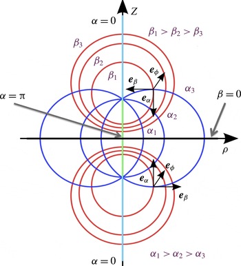
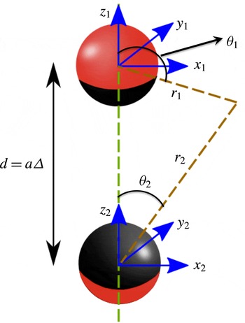
Geometrical sketch of bispherical coordinates
 $({\it\alpha},{\it\beta},{\it\phi})$
.

2 Formulation and analytical solution
Since the key feature here for autonomous motion is the solute concentration field around the colloids, the solute distribution in the presence of both colloids must be captured. Thus, the mass conservation equation for the product solute can be solved in a set of orthogonal curvilinear bispherical coordinates
 $({\it\alpha},{\it\beta},{\it\phi})$
(see figure 1). We assume the colloids have identical radii
 $a$
and their centre-to-centre distance is denoted by
 $d=a{\it\Delta}$
. The colloids are partially active and the extent of their active regions is defined by two angles,
 ${\it\theta}_{cap}^{1}$
and
 ${\it\theta}_{cap}^{2}$
, which vary between
 $0^{\circ }$
and
 $180^{\circ }$
, where
 $0^{\circ }$
accounts for a passive particle while
 $180^{\circ }$
indicates a colloid that is catalytically active over its entire surface. Furthermore, to investigate the relative orientation of the particles, we define a unit orientation vector for each colloid directing from the active to the passive poles. The inclination angles of the two colloids,
 ${\it\Xi}_{1}$
and
 ${\it\Xi}_{2}$
, can be considered as angles between their unit orientation vectors and the positive direction of centre-to-centre line (
 $z$
-direction); these angles varies between
 $0^{\circ }$
and
 $360^{\circ }$
(see figure 2). The motion of the particles is considered to be non-Brownian (
 $t\ll 1/D_{r}$
) and in pseudosteady state and the hydrodynamics is in the Stokes flow regime where the inertial terms can be neglected.
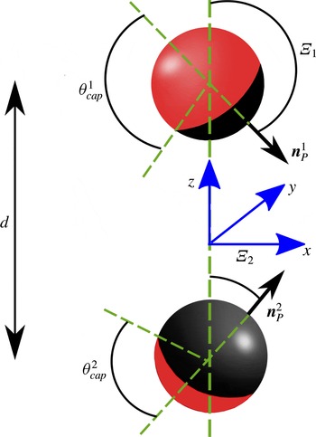
Schematic representation of two catalytically active motors where
 ${\it\theta}_{cap}^{j}$
accounts for the extent of the active region for the colloids,
 $\boldsymbol{n}_{P}^{j}$
is the unit normal directing from active to passive poles and
 ${\it\Xi}_{j}$
determines the relative orientation of the two colloids (
 $j=1$
and
 $2$
).

2.1 Concentration field of product solute
A simple form for the activity of the colloidal particles is taken which consists of a constant flux production of solutes uniformly distributed on the catalytic surface. For small solute in infinite dilution limit, the non-dimensional concentration field of the solute product in the comoving frame can be written as (Khair Reference Khair2013; Michelin & Lauga Reference Michelin and Lauga2014):
 $$\begin{eqnarray}\displaystyle Pe\left(\frac{\partial n}{\partial t}+\boldsymbol{v}\boldsymbol{\cdot }\boldsymbol{{\rm\nabla}}n\right)={\rm\nabla}^{2}n, & & \displaystyle\end{eqnarray}$$
where
 $\boldsymbol{v}$
is the fluid velocity profile,
 $t$
is time and the Péclet number,
 $Pe$
, appears as a direct consequence of non-dimensionalization identifying the relative importance of the time scale for solute advection (
 $a/U_{c}$
) to the time scale for diffusion of product solute (
 $a^{2}/D_{B}$
). At small Péclet numbers (
 $Pe\ll 1$
), the left-hand side of the above equation can be neglected and hence we have the diffusion equation which can be written as,
 $$\begin{eqnarray}\displaystyle {\rm\nabla}^{2}n=0, & & \displaystyle\end{eqnarray}$$
with the following boundary conditions,
 $$\begin{eqnarray}\displaystyle & \displaystyle \boldsymbol{e}_{n}^{j}\boldsymbol{\cdot }\boldsymbol{{\rm\nabla}}n=-{\it\vartheta}_{j}u_{j}(\boldsymbol{r}),\quad \boldsymbol{r}\in S_{c}^{j},(j=1,2), & \displaystyle\end{eqnarray}$$
 $$\begin{eqnarray}\displaystyle & \displaystyle n\rightarrow 0,\quad (\left|\boldsymbol{r}\right|\rightarrow \infty ), & \displaystyle\end{eqnarray}$$
where
 $\boldsymbol{e}_{n}^{j}$
is the unit normal vector pointing outward to the surface of the
 $j$
th colloid,
 $n$
is the non-dimensional concentration of the product solute,
 $\boldsymbol{r}$
is the non-dimensional position vector with respect to the
 $j$
th colloid centre,
 $S_{c}^{j}$
accounts for the surface domain of the
 $j$
th colloid,
 $u_{j}$
is the coverage function of colloid
 $j$
which is one on its active section and zero elsewhere and
 ${\it\vartheta}_{j}$
represents the scaled solute flux production for colloid
 $j$
defined as,
 $$\begin{eqnarray}\displaystyle {\it\vartheta}_{j}=\frac{N_{j}}{N_{1}}, & & \displaystyle\end{eqnarray}$$
where
 $N_{j}$
denotes the dimensional solute flux production for colloid
 $j$
. All variables mentioned above were non-dimensionalized according to the characteristic concentration of the solute
 $n_{c}\sim N_{1}a/D_{B}$
and particle radius
 $a$
. To satisfy the boundary conditions at both colloid surfaces, we utilize a bispherical coordinate
 $({\it\alpha},{\it\beta},{\it\phi})$
. Bispherical coordinates are related to cylindrical coordinates (
 ${\it\rho},{\it\phi},z$
) with the following transformation:
 $$\begin{eqnarray}\displaystyle & \displaystyle {\it\rho}=\frac{c\;\sin {\it\alpha}\;}{\cosh {\it\beta}-\cos {\it\alpha}}, & \displaystyle\end{eqnarray}$$
 $$\begin{eqnarray}\displaystyle & \displaystyle z=\frac{c\;\sinh {\it\beta}}{\cosh {\it\beta}-\cos {\it\alpha}}. & \displaystyle\end{eqnarray}$$
Note that the
 $z$
-axis is always aligned in the direction of the centre-to-centre line of the particles. The range of coordinates are limited to
 $0\leqslant {\it\alpha}\leqslant {\rm\pi}$
,
 ${\it\beta}_{2}<{\it\beta}<{\it\beta}_{1}$
and
 $0\leqslant {\it\phi}\leqslant 2{\rm\pi}$
, for positive scale factor
 $c$
. Furthermore,
 ${\it\beta}={\it\beta}_{1}>0$
represents a sphere whose centre is located on the positive
 $z$
-axis at point
 $z=c\coth {\it\beta}_{1}$
with radius of
 $r_{c1}=c/\sinh {\it\beta}_{1}$
and
 ${\it\beta}={\it\beta}_{2}<0$
is the other sphere whose centre is located on the negative
 $z$
-axis at point
 $z=c\coth {\it\beta}_{2}$
with radius of
 $r_{c2}=c/|\sinh {\it\beta}_{2}|$
(see figure 1 for details). The parameter
 $c$
is non-dimensional and can be related to the separation distance
 $d$
(for two equal spheres) according to,
 $$\begin{eqnarray}\displaystyle & \displaystyle {\it\beta}_{1}=-{\it\beta}_{2}=\cosh ^{-1}\left(\frac{d}{2a}\right), & \displaystyle\end{eqnarray}$$
 $$\begin{eqnarray}\displaystyle & \displaystyle c=\sinh {\it\beta}_{1}. & \displaystyle\end{eqnarray}$$
The general three-dimensional solution of solute distribution in bispherical coordinates can be found via the following ansatz,
 $$\begin{eqnarray}\displaystyle n({\it\alpha},{\it\beta},{\it\phi}) & = & \displaystyle \sqrt{\cosh {\it\beta}-\cos {\it\alpha}}\mathop{\sum }_{m=0}^{\infty }\mathop{\sum }_{n=m}^{\infty }[(\tilde{A}_{nm}\cosh (n+0.5){\it\beta}\nonumber\\ \displaystyle & & \displaystyle +\,\tilde{B}_{nm}\sinh (n+0.5){\it\beta})\cos m{\it\phi}+ (\tilde{C}_{nm}\cosh (n+0.5){\it\beta}\nonumber\\ \displaystyle & & \displaystyle +\,\tilde{D}_{nm}\sinh (n+0.5){\it\beta})\sin m{\it\phi}]P_{n}^{m}(\cos {\it\alpha}),\end{eqnarray}$$
where
 $\tilde{A}_{nm}$
,
 $\tilde{B}_{nm}$
,
 $\tilde{C}_{nm}$
and
 $\tilde{D}_{nm}$
are unknown coefficients that must be determined by applying the boundary conditions on particle surfaces and
 $P_{n}^{m}(\cos {\it\alpha})$
is the associated Legendre function of the first kind. Having utilized the orthogonality of trigonometric functions and the associated Legendre polynomials, we have a set of recursive relationships which must be solved numerically. These relations are given in appendix A.
2.2 Hydrodynamics
The hydrodynamics in the Stokes regime in non-dimensional (see below for non-dimensionalization schemes) form can be written as
 $$\begin{eqnarray}\displaystyle & \displaystyle \boldsymbol{{\rm\nabla}}\boldsymbol{\cdot }\boldsymbol{v}=0, & \displaystyle\end{eqnarray}$$
 $$\begin{eqnarray}\displaystyle & \displaystyle -\boldsymbol{{\rm\nabla}}p+{\rm\nabla}^{2}\boldsymbol{v}=\mathbf{0}, & \displaystyle\end{eqnarray}$$
where
 $p$
is the pressure. The above equations are then subjected to a slip boundary condition at the surfaces of the colloids (
 $j=1$
or
 $2$
) and the quiescent far-field condition while considering the fact that particles are force and torque free
 $$\begin{eqnarray}\displaystyle & \displaystyle \boldsymbol{v}(\boldsymbol{r}\in S_{c}^{j})=\boldsymbol{v}_{s}^{j}+\boldsymbol{U}^{j}+{\it\bf\Omega}^{j}\times (\boldsymbol{r}-\boldsymbol{r}_{0}^{j}), & \displaystyle\end{eqnarray}$$
 $$\begin{eqnarray}\displaystyle & \displaystyle \boldsymbol{v}(\left|\boldsymbol{r}\right|\rightarrow \infty )\rightarrow \mathbf{0}, & \displaystyle\end{eqnarray}$$
 $$\begin{eqnarray}\displaystyle & \displaystyle \boldsymbol{F}_{T}^{j}=\unicode[STIX]{x0222F}_{S_{c}^{j}}(\boldsymbol{e}_{n}^{j}\boldsymbol{\cdot }{\bf\sigma})\,\text{d}S=\mathbf{0}, & \displaystyle\end{eqnarray}$$
 $$\begin{eqnarray}\displaystyle & \displaystyle \boldsymbol{T}_{T}^{j}=\unicode[STIX]{x0222F}_{S_{c}^{j}}(\boldsymbol{r}-\boldsymbol{r}_{0}^{j})\times (\boldsymbol{e}_{n}^{j}\boldsymbol{\cdot }{\bf\sigma})\,\text{d}S=\mathbf{0}, & \displaystyle\end{eqnarray}$$
where
 ${\bf\sigma}$
is the stress tensor,
 $\boldsymbol{r}_{0}^{j}$
is the location of the
 $j$
th particle centre of mass,
 $\boldsymbol{U}^{j}$
and
 ${\it\bf\Omega}^{j}$
are the non-dimensional translational and angular velocities of the
 $j$
th colloid yet to be determined and finally
 $\boldsymbol{v}_{s}^{j}$
is the non-dimensional slip velocity on the surface of the
 $j$
th colloidal motor, given as
 $$\begin{eqnarray}\displaystyle \boldsymbol{v}_{s}^{j}=-\boldsymbol{{\rm\nabla}}_{s}\,n(\boldsymbol{r}\in S_{c}^{j}), & & \displaystyle\end{eqnarray}$$
where the surface gradient is defined as
 $\boldsymbol{{\rm\nabla}}_{s}=(\boldsymbol{I}-\boldsymbol{e}_{n}\boldsymbol{e}_{n})\boldsymbol{\cdot }\boldsymbol{{\rm\nabla}}$
and all variables introduced in the above were non-dimensionalized with
 $U_{c}\sim bn_{c}/a$
,
 ${\it\Omega}_{c}\sim bn_{c}/a^{2}$
,
 $p$
and
 ${\bf\sigma}\sim {\it\mu}U_{c}/a$
,
 $F_{c}\sim {\it\mu}U_{c}a$
and
 $T_{c}\sim {\it\mu}U_{c}a^{2}$
. The mobility coefficient
 $b$
is defined as
 $$\begin{eqnarray}\displaystyle b=\frac{k_{B}TL^{2}}{{\it\mu}}\int _{0}^{\infty }y^{\prime }\left[\exp \left(-\frac{{\it\psi}}{k_{B}T}\right)-1\right]\text{d}y^{\prime }, & & \displaystyle\end{eqnarray}$$
where
 ${\it\mu}$
is the fluid viscosity,
 $k_{B}$
is the Boltzmann constant,
 $T$
is the absolute fluid temperature,
 $y^{\prime }$
is the distance to the particle edge and
 ${\it\psi}$
is the net potential interaction of the solute molecules with the particle in the presence of solvent. For a hard-sphere potential between solutes and colloids, this reduces to
 $b=-k_{B}TL^{2}/2{\it\mu}$
.
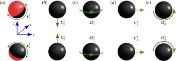
Decomposition of velocity field into (a) surface diffusiophoretic slip with no net movement (translational or rotational) of the colloids (b) translation of colloids parallel to the line of centres (
 $z$
axis) with no rotation or slip (c) rotation of colloids around the line of centres (
 $z$
axis) with no slip or translation (d) translation of colloids perpendicular to the line of centres (
 $x$
or
 $y$
axis) with no slip or rotation (e) rotation of colloids around the third axis (
 $y$
or
 $x$
axis) with no slip or translation.

The arbitrary motion of two colloidal particles in space can be decomposed into translational motion parallel
 $\Vert$
(
 $z$
-axis) and perpendicular
 $\bot$
(
 $x$
- and
 $y$
-axes) to the line of centres and rotational motion around an axis parallel
 $\Vert$
(
 $z$
-axis) to the line of centres and the third axis
 $\otimes$
(
 $y$
- and
 $x$
-axes), (see figure 3 for details). Furthermore, due to linearity of the Stokes flow equations and the boundary conditions, the fluid flow around two catalytically active particles can be decomposed into five subproblems (see figure 3):
-
(i) The colloidal particles are stationary, i.e.
 $U_{\Vert }^{j}=U_{\bot }^{j}={\it\Omega}_{\Vert }^{j}={\it\Omega}_{\otimes }^{j}=0$
and
$j=1$
,
$2$
, but the fluid slips according to the diffusiophoretic slip (2.17) on particles surfaces.
-
(ii) The colloidal particles are translating with velocities
$U_{\Vert }^{1}$
and
$U_{\Vert }^{2}$
parallel to the line of centres (
$z$
-direction) with no translations along the axis perpendicular to the line of centres (
$U_{\bot }^{1}=U_{\bot }^{2}=0$
) or rotations around any axes (
${\it\Omega}_{\Vert }^{j}={\it\Omega}_{\otimes }^{j}=0$
). In this case, the colloids experience hydrodynamic forces in the direction of motion
$F_{\Vert }^{j,H}$
, but the motion is axisymmetric and hence there are no hydrodynamic torques on particles. -
(iii) The colloidal particles are rotating with angular velocities
${\it\Omega}_{\Vert }^{1}$
and
${\it\Omega}_{\Vert }^{2}$
around the axis parallel to the line of centres (
$z$
-direction) with no translations along any direction (
$U_{\Vert }^{j}=U_{\bot }^{j}=0$
) or rotations around any other axes (
${\it\Omega}_{\otimes }^{1}={\it\Omega}_{\otimes }^{2}=0$
). In this case, the colloids experience hydrodynamic torques
$T_{\Vert }^{j,H}$
, but their motions are axisymmetric and hence there are no hydrodynamic forces on the particles. We will show below that this contribution is identically zero in self-diffusiophoresis. -
(iv) The colloidal particles are translating with velocities
$U_{\bot }^{1}$
and
$U_{\bot }^{2}$
along an axis perpendicular to the line of centres with no translations along the axis parallel to the line of centres (
$U_{\Vert }^{1}=U_{\Vert }^{2}=0$
) or rotations around any other axes (
${\it\Omega}_{\Vert }^{j}={\it\Omega}_{\otimes }^{j}=0$
). In this case, due to the hydrodynamic coupling between the motions of the particles, there are hydrodynamic forces in the direction of motion and torques around an axis along the third direction. -
(v) The colloidal particles are rotating with angular velocities
${\it\Omega}_{\otimes }^{1}$
and
${\it\Omega}_{\otimes }^{2}$
around the third axis with no translations along any axis (
$U_{\Vert }^{j}=U_{\bot }^{j}=0$
) or rotations around the axis parallel to the line of centres (
${\it\Omega}_{\Vert }^{1}={\it\Omega}_{\Vert }^{2}=0$
). In this case, due to the hydrodynamic coupling between the motions of the particles, there are hydrodynamic forces in a direction perpendicular to the line of centres.



Note that in the above decomposition, each one of problems (iv) and (v) are generally two problems (one along
 $x$
and the other along
 $y$
-directions); nonetheless, the treatment for both are identical. To obtain the swimming velocities of the active colloids, the forces and torques associated with each one of the above five problems should be determined. Additionally, analytical expressions of hydrodynamic forces and torques on two particles for problems (ii)–(v) have already been derived in the literature (Jeffery Reference Jeffery1915; Stimson & Jeffery Reference Stimson and Jeffery1926; Maude Reference Maude1961; Goldman, Cox & Brenner Reference Goldman, Cox and Brenner1966; Wakiya Reference Wakiya1967; Davis Reference Davis1969; O’Neill & Majumdar Reference O’Neill and Majumdar1970a
; Spielman Reference Spielman1970) and (in a general linear form) can be written as
 $$\begin{eqnarray}\displaystyle \boldsymbol{F}^{H}=-\unicode[STIX]{x1D64D}\boldsymbol{\cdot }\boldsymbol{U}, & & \displaystyle\end{eqnarray}$$
where
 $\unicode[STIX]{x1D64D}$
(a
 $12\times 12$
matrix) is the grand resistance matrix,
 $\boldsymbol{F}^{H}$
is the
 $12$
-component vector including the hydrodynamic forces and torques on two particles and the
 $12$
-component vector
 $\boldsymbol{U}$
contains the translational and rotational velocities (
 $\boldsymbol{U}^{j}$
and
 ${\it\bf\Omega}^{j}$
) of the particles in Cartesian coordinates. Having known that both colloids are force and torque free, i.e.
 $\boldsymbol{F}^{H}+\boldsymbol{F}^{P}=0$
, the swimming translational and rotational velocities of the particles are linearly related to the propulsive (diffusiophoretic) forces and torques (problem (i) in the above decomposition) through the grand mobility matrix
 $\unicode[STIX]{x1D64D}^{-1}$
which in general form can be given as
 $$\begin{eqnarray}\displaystyle \boldsymbol{U}=\unicode[STIX]{x1D64D}^{-1}\boldsymbol{\cdot }\boldsymbol{F}^{P}, & & \displaystyle\end{eqnarray}$$
where
 $\boldsymbol{F}^{P}$
is the
 $12$
-component vector including the propulsive forces and torques on two particles (force and torques on particles in figure 3
a). To obtain
 $\boldsymbol{U}$
and eventually the trajectory of swimmers, the only task that has to be done is to evaluate the propulsive forces and torques
 $\boldsymbol{F}^{P}$
. This can be achieved by utilizing the analytical solution for Stokes flow in bispherical coordinates (Lee & Leal Reference Lee and Leal1980). In this case, the velocity components are in terms of infinite series with coefficients that must be found numerically. Thereafter, the forces and torques on the particles associated with problem (i) in figure 3(a) can be numerically calculated. This method has been used in a number of studies, including ones involving the dynamics of two spherical particles, a spherical particle in the vicinity of a planar solid wall in electrophoresis (Keh & Chen Reference Keh and Chen1988; Zeng, Zinchenko & Davis Reference Zeng, Zinchenko and Davis1999) and the self-diffusiophoresis of a catalytic particle near a solid wall (Mozaffari et al.
Reference Mozaffari, Sharifi-Mood, Koplik and Maldarelli2016). This approach is straightforward, however the details of the calculation and algebra are cumbersome and hence our objective here is to employ an alternative approach to obtain expressions for swimming translational and angular velocities
 $\boldsymbol{U}^{j}$
and
 ${\it\bf\Omega}^{j}$
of the particles due to self-diffusiophoresis. Here, we use the RRT (Teubner Reference Teubner1982; Happel & Brenner Reference Happel and Brenner1983; Stone & Samuel Reference Stone and Samuel1996; Masoud & Stone Reference Masoud and Stone2014) to simplify the calculation of propulsive forces and torques on particles as explicit integrals in terms of the stress tensor of classical Stokes flow problems involving translational and rotational motion of two spherical particles. A significant advantage of RRT is that the hydrodynamics (2.11) and (2.12) does not need to be solved in order to evaluate the force and torque and therefore the calculations is significantly reduced.
Suppose (
 $\boldsymbol{v}^{\prime },{\bf\sigma}^{\prime }$
) and (
 $\boldsymbol{v}^{\prime \prime },{\bf\sigma}^{\prime \prime }$
) are the solutions of the Stokes flow of an incompressible fluid for some arbitrary fluid volume
 ${\it\Sigma}$
. According to RRT, one can state that:
 $$\begin{eqnarray}\displaystyle \unicode[STIX]{x0222F}_{\partial {\it\Sigma}}\boldsymbol{n}_{{\it\Sigma}}\boldsymbol{\cdot }{\bf\sigma}^{\prime }\boldsymbol{\cdot }\boldsymbol{v}^{\prime \prime }\,\text{d}S=\unicode[STIX]{x0222F}_{\partial {\it\Sigma}}\boldsymbol{n}_{{\it\Sigma}}\boldsymbol{\cdot }{\bf\sigma}^{\prime \prime }\boldsymbol{\cdot }\boldsymbol{v}^{\prime }\,\text{d}S, & & \displaystyle\end{eqnarray}$$
where
 $\partial {\it\Sigma}$
represents the boundaries enclosing the volume
 ${\it\Sigma}$
; for instance, in the case of two spherical colloids,
 $\partial {\it\Sigma}$
accounts for a union of the boundaries including the colloids surfaces and an enclosing surface boundary far away from the two colloids, where
 $\boldsymbol{n}_{{\it\Sigma}}$
are the unit normals on these boundaries. Inasmuch as the velocity field of the test problem around the colloidal particles attenuates as
 $v\sim |\boldsymbol{r}|^{-1}$
or faster, the far-field area integral does not contribute to the calculation and can be neglected.
Having utilized RRT to evaluate the propulsive forces and torques on the particles
 $\boldsymbol{F}^{P}$
(see below for detail), we can substitute the propulsive forces and torques on the particle in (2.20) to construct a compact formula which express swimming translational and angular velocities of the particles according to (see Stone & Samuel Reference Stone and Samuel1996; Elfring Reference Elfring2015; Elfring & Lauga Reference Elfring and Lauga2015)
 $$\begin{eqnarray}\displaystyle \boldsymbol{U}=\unicode[STIX]{x1D64D}^{-1}\boldsymbol{\cdot }\mathop{\sum }_{j=1}^{2}\unicode[STIX]{x0222F}_{S_{c}^{j}}\boldsymbol{v}_{s}^{j}\boldsymbol{\cdot }(\boldsymbol{e}_{n}^{j}\boldsymbol{\cdot }\unicode[STIX]{x1D64F})\,\text{d}s, & & \displaystyle\end{eqnarray}$$
where
 $\unicode[STIX]{x1D64F}$
denotes the triadic hydrodynamic stress fields (a
 $[3\times 3]\times 12$
matrix) associated with translations and rotations of two spherical particles and note that in the above expression we utilized the linearity of the Stokes equations by letting
 ${\bf\sigma}^{\prime \prime }=\unicode[STIX]{x1D64F}\boldsymbol{\cdot }\boldsymbol{U}$
. Below we evaluate the integral in (2.22) to discuss the propulsive forces and torques on particles in different directions.
2.2.1 Propulsive forces on two colloidal motors along the centre-to-centre line
To quantify the forces on the particles along the line of centres (
 $z$
-direction), (
 $\boldsymbol{v}^{\prime \prime }$
,
 ${\bf\sigma}^{\prime \prime }$
) in (2.21) is chosen to be the solution of translational motion of two colloids along their line of centres which satisfies the following boundary conditions at the particle surfaces and far field,
 $$\begin{eqnarray}\displaystyle & \displaystyle \boldsymbol{v}^{\prime \prime }(\boldsymbol{r}\in S_{c}^{j})=\boldsymbol{e}_{\Vert },\quad (j=1,2), & \displaystyle\end{eqnarray}$$
 $$\begin{eqnarray}\displaystyle & \displaystyle \boldsymbol{v}^{\prime \prime }(|\boldsymbol{r}|\rightarrow \infty )=\mathbf{0}, & \displaystyle\end{eqnarray}$$
where
 $\boldsymbol{e}_{\Vert }$
is the unit normal vector along the line of centres. This problem was analysed in detail by Stimson & Jeffery (Reference Stimson and Jeffery1926). Having substituted (
 $\boldsymbol{v}^{\prime \prime }$
,
 ${\bf\sigma}^{\prime \prime }$
) in (2.21), it can be shown that
 $$\begin{eqnarray}\displaystyle F_{\Vert }^{1,P}+F_{\Vert }^{2,P}=\unicode[STIX]{x0222F}_{S_{c}^{1}}\boldsymbol{e}_{{\it\beta}}\boldsymbol{\cdot }{\bf\sigma}_{S-J}\boldsymbol{\cdot }\boldsymbol{{\rm\nabla}}_{s}n\,\text{d}S-\unicode[STIX]{x0222F}_{S_{c}^{2}}\boldsymbol{e}_{{\it\beta}}\boldsymbol{\cdot }{\bf\sigma}_{S-J}\boldsymbol{\cdot }\boldsymbol{{\rm\nabla}}_{s}n\,\text{d}S, & & \displaystyle\end{eqnarray}$$
where
 ${\bf\sigma}_{S-J}$
is the stress tensor corresponding to the Stimson & Jeffery (Reference Stimson and Jeffery1926) analysis. At the moment we have one equation (2.25) with two unknowns (
 $F_{\Vert }^{1,P}$
and
 $F_{\Vert }^{2,P}$
) and hence one more equation is required to close the problem. To obtain the second relationship, RRT can be used one more time by assuming (
 $\boldsymbol{v}^{\prime \prime }$
,
 ${\bf\sigma}^{\prime \prime }$
) in (2.21) is the solution of translational motion of two colloids along their line of centres and which translate in an opposite direction,
 $$\begin{eqnarray}\boldsymbol{v}^{\prime \prime }(\boldsymbol{r}\in S_{c}^{j})=\mp \boldsymbol{e}_{\Vert },(j=1,2),\end{eqnarray}$$
 $$\begin{eqnarray}\boldsymbol{v}^{\prime \prime }(|\boldsymbol{r}|\rightarrow \infty )=\mathbf{0},\end{eqnarray}$$
where the minus sign in (2.26) is for particle
 $1$
on top and the plus sign is for the particle
 $2$
on the bottom. This problem was analysed initially by Maude (Reference Maude1961) (but with some errors) and, by substitution of the solution, we have
 $$\begin{eqnarray}\displaystyle -F_{\Vert }^{1,P}+F_{\Vert }^{2,P}=\unicode[STIX]{x0222F}_{S_{c}^{1}}\boldsymbol{e}_{{\it\beta}}\boldsymbol{\cdot }{\bf\sigma}_{M}\boldsymbol{\cdot }\boldsymbol{{\rm\nabla}}_{s}n\,\text{d}S-\unicode[STIX]{x0222F}_{S_{c}^{2}}\boldsymbol{e}_{{\it\beta}}\boldsymbol{\cdot }{\bf\sigma}_{M}\boldsymbol{\cdot }\boldsymbol{{\rm\nabla}}_{s}n\,\text{d}S, & & \displaystyle\end{eqnarray}$$
where
 ${\bf\sigma}_{M}$
is the stress tensor corresponding to the Maude (Reference Maude1961) analysis. Having solved equations (2.25) and (2.28) simultaneously, the two unknowns
 $F_{z}^{1,P}$
and
 $F_{z}^{2,P}$
can be evaluated. Note that the above integrals were calculated numerically to find the magnitude of the propulsive forces along the line of centres (
 $z$
-direction) of the two colloids.
2.2.2 Propulsive torques on two colloidal motors parallel to their line of centres
Propulsive torques on colloids around the line of centres (
 $z$
-axis) can be directly evaluated with RRT by letting (
 $\boldsymbol{v}^{\prime \prime }$
,
 ${\bf\sigma}^{\prime \prime }$
) in (2.21) be the solution of the rotations of the two colloids around their line of centres. This analysis was performed by Jeffery (Reference Jeffery1915) and it is reiterated in appendix B. In this case, the problem is axisymmetric and the only non-zero component of the velocity field is in the azimuthal angle direction
 ${\it\phi}$
, and hence all non-zero components of the stress tensor associated with this problem do not have a
 ${\it\phi}$
dependency. On the other hand, the solute concentration gradient does depend on
 ${\it\phi}$
and hence the propulsive torques on colloids along the line of centres can be proven to be identically zero,
 $$\begin{eqnarray}\displaystyle T_{\Vert }^{j,P}=\mp \unicode[STIX]{x0222F}_{S_{c}^{j}}\boldsymbol{e}_{{\it\beta}}\boldsymbol{\cdot }{\bf\sigma}_{J}\boldsymbol{\cdot }\boldsymbol{{\rm\nabla}}_{s}n\;\text{d}S=0, & & \displaystyle\end{eqnarray}$$
where
 ${\bf\sigma}_{J}$
is the non-dimensional stress tensor associated with Jeffery’s problem.
2.2.3 Propulsive forces and torques on two colloidal motors perpendicular to their line of centres and around the third axis
In this case, the propulsive forces and torques on colloidal particles are in a direction perpendicular to the line of centres and around the third axis respectively. These directions can be either in
 $x$
or
 $y$
(see figure 2) and the analysis for each one of the directions is similar. The translational (or rotational) motion of colloidal particles in this case is no longer axisymmetric and the colloids experience a torque (or force) in the
 $y$
(or
 $x$
) direction.
To use RRT (2.21) for calculation of the propulsive forces and torques on the colloids, (
 $\boldsymbol{v}^{\prime \prime }$
,
 ${\bf\sigma}^{\prime \prime }$
) is chosen to be the solution of four subproblems:
(I) Two colloids are translating with no rotation in the same direction with a unit velocity perpendicular to the line of centres
 $$\begin{eqnarray}\displaystyle & \displaystyle \boldsymbol{v}^{\prime \prime }(\boldsymbol{r}\in S_{c}^{1})=\boldsymbol{e}_{\bot }, & \displaystyle\end{eqnarray}$$
 $$\begin{eqnarray}\displaystyle & \displaystyle \boldsymbol{v}^{\prime \prime }(\boldsymbol{r}\in S_{c}^{2})=\boldsymbol{e}_{\bot }, & \displaystyle\end{eqnarray}$$
 $$\begin{eqnarray}\displaystyle & \displaystyle \boldsymbol{v}^{\prime \prime }(|\boldsymbol{r}|\rightarrow \infty )=\mathbf{0}, & \displaystyle\end{eqnarray}$$
where
 $\boldsymbol{e}_{\bot }$
can be either
 $\boldsymbol{e}_{x}$
or
 $\boldsymbol{e}_{y}$
. This problem was analysed by Goldman et al. (Reference Goldman, Cox and Brenner1966). Having utilized RRT (2.21), one can show
 $$\begin{eqnarray}\displaystyle F_{\bot }^{1,P}+F_{\bot }^{2,P}=\unicode[STIX]{x0222F}_{S_{c}^{1}}\boldsymbol{e}_{{\it\beta}}\boldsymbol{\cdot }\tilde{{\bf\sigma}_{1}}\boldsymbol{\cdot }\boldsymbol{{\rm\nabla}}_{s}n\,\text{d}S-\unicode[STIX]{x0222F}_{S_{c}^{2}}\boldsymbol{e}_{{\it\beta}}\boldsymbol{\cdot }\tilde{{\bf\sigma}_{1}}\boldsymbol{\cdot }\boldsymbol{{\rm\nabla}}_{s}n\,\text{d}S, & & \displaystyle\end{eqnarray}$$
where
 $\tilde{{\bf\sigma}}_{1}$
is the non-dimensional stress tensor corresponding to analysis in Goldman et al. (Reference Goldman, Cox and Brenner1966).
(II) Two colloids are rotating with no translation in opposite directions around the third direction which can be either the
 $y$
- or
 $x$
-axis,
 $$\begin{eqnarray}\displaystyle & \displaystyle \boldsymbol{v}^{\prime \prime }(\boldsymbol{r}\in S_{c}^{1})=\boldsymbol{e}_{\otimes }\times (\boldsymbol{r}-\boldsymbol{r}_{0}^{1}), & \displaystyle\end{eqnarray}$$
 $$\begin{eqnarray}\displaystyle & \displaystyle \boldsymbol{v}^{\prime \prime }(\boldsymbol{r}\in S_{c}^{2})=-\boldsymbol{e}_{\otimes }\times (\boldsymbol{r}-\boldsymbol{r}_{0}^{2}), & \displaystyle\end{eqnarray}$$
 $$\begin{eqnarray}\displaystyle & \displaystyle \boldsymbol{v}^{\prime \prime }(|\boldsymbol{r}|\rightarrow \infty )=\mathbf{0}, & \displaystyle\end{eqnarray}$$
where
 $\boldsymbol{e}_{\otimes }$
accounts for the unit vector in the third direction, i.e.
 $y$
or
 $x$
. This problem was also analysed by Goldman et al. (Reference Goldman, Cox and Brenner1966). Having utilized RRT (2.21), one can show
 $$\begin{eqnarray}\displaystyle T_{\otimes }^{1,P}-T_{\otimes }^{2,P}=\unicode[STIX]{x0222F}_{S_{c}^{1}}\boldsymbol{e}_{{\it\beta}}\boldsymbol{\cdot }\tilde{{\bf\sigma}_{2}}\boldsymbol{\cdot }\boldsymbol{{\rm\nabla}}_{s}n\,\text{d}S-\unicode[STIX]{x0222F}_{S_{c}^{2}}\boldsymbol{e}_{{\it\beta}}\boldsymbol{\cdot }\tilde{{\bf\sigma}_{2}}\boldsymbol{\cdot }\boldsymbol{{\rm\nabla}}_{s}n\,\text{d}S, & & \displaystyle\end{eqnarray}$$
where
 $\tilde{{\bf\sigma}}_{2}$
is the non-dimensional stress tensor corresponding to the analysis performed by Goldman et al. (Reference Goldman, Cox and Brenner1966).
(III) Two colloids are translating with no rotation in an opposite direction with a unit velocity perpendicular to the line of centres,
 $$\begin{eqnarray}\displaystyle & \displaystyle \boldsymbol{v}^{\prime \prime }\left(\boldsymbol{r}\in S_{c}^{1}\right)=\boldsymbol{e}_{\bot }, & \displaystyle\end{eqnarray}$$
 $$\begin{eqnarray}\displaystyle & \displaystyle \boldsymbol{v}^{\prime \prime }\left(\boldsymbol{r}\in S_{c}^{2}\right)=-\boldsymbol{e}_{\bot }, & \displaystyle\end{eqnarray}$$
 $$\begin{eqnarray}\displaystyle & \displaystyle \boldsymbol{v}^{\prime \prime }\left(|\boldsymbol{r}|\rightarrow \infty \right)=\mathbf{0}. & \displaystyle\end{eqnarray}$$
This problem was analysed by O’Neill (Reference O’Neill1969). Having utilized RRT (2.21), we find
 $$\begin{eqnarray}\displaystyle F_{\bot }^{1,P}-F_{\bot }^{2,P}=\unicode[STIX]{x0222F}_{S_{c}^{1}}\boldsymbol{e}_{{\it\beta}}\boldsymbol{\cdot }\tilde{{\bf\sigma}_{3}}\boldsymbol{\cdot }\boldsymbol{{\rm\nabla}}_{s}n\,\text{d}S-\unicode[STIX]{x0222F}_{S_{c}^{2}}\boldsymbol{e}_{{\it\beta}}\boldsymbol{\cdot }\tilde{{\bf\sigma}_{3}}\boldsymbol{\cdot }\boldsymbol{{\rm\nabla}}_{s}n\,\text{d}S, & & \displaystyle\end{eqnarray}$$
where
 $\tilde{{\bf\sigma}}_{3}$
is the non-dimensional stress tensor corresponding to the analysis performed by O’Neill (Reference O’Neill1969).
(IV) Two colloids are rotating with no translation in the same direction
 $$\begin{eqnarray}\displaystyle & \displaystyle \boldsymbol{v}^{\prime \prime }\left(\boldsymbol{r}\in S_{c}^{1}\right)=\boldsymbol{e}_{\otimes }\times \left(\boldsymbol{r}-\boldsymbol{r}_{0}^{1}\right), & \displaystyle\end{eqnarray}$$
 $$\begin{eqnarray}\displaystyle & \displaystyle \boldsymbol{v}^{\prime \prime }\left(\boldsymbol{r}\in S_{c}^{2}\right)=\boldsymbol{e}_{\otimes }\times \left(\boldsymbol{r}-\boldsymbol{r}_{0}^{2}\right), & \displaystyle\end{eqnarray}$$
 $$\begin{eqnarray}\displaystyle & \displaystyle \boldsymbol{v}^{\prime \prime }\left(|\boldsymbol{r}|\rightarrow \infty \right)=\mathbf{0}. & \displaystyle\end{eqnarray}$$
This problem was also analysed by O’Neill (Reference O’Neill1969). Having utilized RRT (2.21), we find
 $$\begin{eqnarray}\displaystyle T_{\otimes }^{1,P}+T_{\otimes }^{2,P}=\unicode[STIX]{x0222F}_{S_{c}^{1}}\boldsymbol{e}_{{\it\beta}}\boldsymbol{\cdot }\tilde{{\bf\sigma}_{4}}\boldsymbol{\cdot }\boldsymbol{{\rm\nabla}}_{s}n\,\text{d}S-\unicode[STIX]{x0222F}_{S_{c}^{2}}\boldsymbol{e}_{{\it\beta}}\boldsymbol{\cdot }\tilde{{\bf\sigma}_{4}}\boldsymbol{\cdot }\boldsymbol{{\rm\nabla}}_{s}n\,\text{d}S, & & \displaystyle\end{eqnarray}$$
where
 $\tilde{{\bf\sigma}}_{4}$
is the non-dimensional stress tensor corresponding to the O’Neill (Reference O’Neill1969) analysis.
By combining equations (2.33) and (2.41) and (2.37) and (2.45), the forces and torques around the third axis can be evaluated respectively.
The solution to the four classical problems (Goldman et al.
Reference Goldman, Cox and Brenner1966; O’Neill Reference O’Neill1969) mentioned above are reiterated in appendix B. The above relations provide forces and torques on the particles in (2.20) and the integral on the right-hand side of (2.22). The integrands were all evaluated according to the analytical relations, however, the integrations were performed numerically. In the evaluation of these quadratures, all stress tensors associated with the classical problems are in the form of infinite sums and, in our calculation, these series are truncated according to the fact that the coefficients vanish for sufficiently large number of terms. Also, more terms in the truncated series were required for small separation distances to reach numerically accurate and consistent results for both concentration field and stress tensor components. Once the propulsive forces and torques on the particles
 $\boldsymbol{F}^{P}$
are known, we can utilize the mobility relation given in (2.22) (or alternatively (2.20)) to obtain swimming translational and angular velocity of the particles.
3 Results and discussion
At a given separation distance, the dynamics of two catalytic motors depends on colloids coverage
 ${\it\theta}_{cap}^{j}$
and their relative orientation
 $\boldsymbol{n}_{P}^{j}$
. Here, we consider the case where the orientation vectors are in the same plane and we choose this to be the
 $x$
–
 $z$
plane. Furthermore, a net repulsive hard-sphere excluded volume interaction is considered between product solute and colloids in the presence of solvent so that the particles swim along their orientation vectors when they are far away from each other.
3.1 Concentration field
The solute concentration field around the colloids is independent of azimuthal angle
 ${\it\phi}$
when the inclination angles of the colloids are either
 $0^{\circ }$
or
 $180^{\circ }$
. For the situation where the active sections of colloids are opposite to each other, i.e.
 ${\it\Xi}_{1}=180^{\circ }$
and
 ${\it\Xi}_{2}=0^{\circ }$
, the solute distribution does not change drastically, except for very high coverage, as the colloids approach each other since the solutes can freely diffuse away from them (see figure 4
a,d). By contrast, in the other case where the active caps of the colloids face towards each other,
 ${\it\Xi}_{1}=0^{\circ }$
and
 ${\it\Xi}_{2}=180^{\circ }$
, as the separation distance between the particle decreases, the concentration of solute increases precipitously in the gap region adjacent to the colloids (see figure 4
b,e). When the active section of one colloid faces the passive section of the other one, i.e.
 ${\it\Xi}_{1}={\it\Xi}_{2}=0^{\circ }$
, the concentration of solute in the gap increases again as the separation distance between the colloids decreases. The major difference between this situation and the other two previous axisymmetric cases is the fact that the concentration field is no longer symmetric with respect to the midplane
 $x$
–
 $y$
and hence, as we show later, the swimming velocities of the colloids are no longer equal in magnitude (see figure 4
c,f).
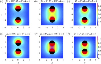
Non-dimensional concentration field for half active Janus colloids
 $({\it\theta}_{cap}^{1}={\it\theta}_{cap}^{2}=90^{\circ })$
in the
 $x$
–
 $z$
plane for axisymmetric orientation of colloids with
 ${\it\Xi}_{1}=180^{\circ }$
and
 ${\it\Xi}_{2}=0^{\circ }$
at two different non-dimensional centre-to-centre distances of (a)
 ${\it\Delta}=4$
and (d)
 ${\it\Delta}=3$
, and
 ${\it\Xi}_{1}=0^{\circ }$
and
 ${\it\Xi}_{2}=180^{\circ }$
at (b)
 ${\it\Delta}=4$
and (e)
 ${\it\Delta}=3$
, and
 ${\it\Xi}_{1}={\it\Xi}_{2}=0^{\circ }$
at (c)
 ${\it\Delta}=4$
and (f)
 ${\it\Delta}=3$
. Note that the red caps indicate the catalytic surface of the colloids.

For all other orientations, the solution of the concentration field is three-dimensional in bispherical coordinates,
 $n\left({\it\alpha},{\it\beta},{\it\phi}\right)$
. Representative concentration fields in the
 $x$
–
 $z$
plane around two Janus colloids
 $({\it\theta}_{cap}^{1}={\it\theta}_{cap}^{2}=90)$
for various relative inclination angles and a fixed separation distance
 ${\it\Delta}=3$
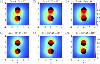
are shown in figure 5. The pair interaction effect is more pronounced when the active sections are close to each other and therefore the solute concentration is boosted in the gap. Furthermore, for all values of the inclination angles except the symmetric cases, the concentration fields around the colloids are no longer symmetric with respect to the centre-to-centre line (see figure 5) and hence results in the rotation of particles. These rotations are the direct consequence of diffusiophoresis, which is due to the asymmetric distribution of product solute; this effect will be discussed in detail presently. Furthermore, the asymmetric distribution around the colloid axis is more pronounced as the inclination angles of colloids approach
 ${\it\Xi}_{j}\rightarrow 90^{\circ }$
or
 ${\it\Xi}_{j}\rightarrow 270^{\circ }$
(
 $j=1,2$
).
Non-dimensional concentration field for half active Janus colloids
 $({\it\theta}_{cap}^{1}={\it\theta}_{cap}^{2}=90^{\circ })$
in the
 $x$
–
 $z$
plane for asymmetric orientations and non-dimensional centre-to-centre distance of
 ${\it\Delta}=3$
. Note that the red caps indicate the catalytic surface of the colloids.

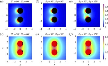
The concentration field around colloids can be altered not only by changing the orientation of colloids but also by varying the extent of the active sections. Figure 6(a–c) demonstrates concentration fields in the
 $x$
–
 $z$
plane for small (
 ${\it\theta}_{cap}^{1}={\it\theta}_{cap}^{2}=40^{\circ }$
) and large (
 ${\it\theta}_{cap}^{1}={\it\theta}_{cap}^{2}=140^{\circ }$
) active coverages. Note that for
 ${\it\theta}_{cap}^{j}=140^{\circ }$
, there is a substantial increase in solute concentration in the gap relative to the case where
 ${\it\theta}_{cap}^{j}=40^{\circ }$
for similar inclination angles. Thus, the diffusiophoretic effect for colloids with large active coverage is more significant compared to the colloids with smaller coverage.
Non-dimensional concentration field for active colloids at various inclination angles in the
 $x$
–
 $z$
plane for asymmetric orientation of colloids at non-dimensional centre-to-centre distance of
 ${\it\Delta}=3$
with (a–c)
 ${\it\theta}_{cap}^{1}={\it\theta}_{cap}^{2}=40^{\circ }$
and (d–f)
 ${\it\theta}_{cap}^{1}={\it\theta}_{cap}^{2}=140^{\circ }$
. Note that the red caps indicate the catalytic surface of the colloids.

3.2 Swimming velocities and trajectories
3.2.1 Axisymmetric motion of two colloidal motors swimming in the direction parallel to the centre-to-centre line
To study the hydrodynamics of colloidal self-propulsion, we first focus on the axisymmetric motion of two motors, i.e. the inclination angles of the colloids are either
 $0^{\circ }$
or
 $180^{\circ }$
. In this situation, the only non-zero component of the swimming velocity is in the
 $z$
-direction (see figure 2). Moreover, since the flow is axisymmetric, the colloids do not undergo a rotation around any axis. This condition simplifies the governing equations significantly and the flow field can be found by using the conventional streamfunction technique in bispherical coordinates for the Stokes flow regime (Popescu et al.
Reference Popescu, Tasinkevych and Dietrich2011; Sharifi-Mood Reference Sharifi-Mood2013; Reigh & Kapral Reference Reigh and Kapral2015). Additionally, to obtain a far-field solution, we employ a method of reflections to validate our analytical solution. The detailed derivation of this solution is discussed in appendix C.
Non-dimensional swimming velocities of two half active Janus colloidal motors (
 ${\it\theta}_{cap}^{1}={\it\theta}_{cap}^{2}=90^{\circ }$
) as a function of non-dimensional separation distance
 ${\it\Delta}-2$
for axisymmetric motions. Open symbols represent the full solution while the solid lines are the results from the method of reflections.

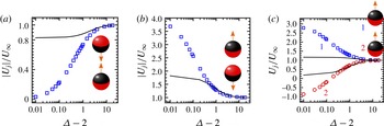
Figure 7 illustrates the non-dimensional swimming velocities of two Janus colloids as a function of the centre-to-centre separation distance
 ${\it\Delta}$
for three relative orientations. In all cases, the colloids move along the centre-to-centre line (
 $z$
-direction), however, the dependency of the swimming velocities on the separation distance are substantially different for them. The concentration field can be symmetric or asymmetric with respect to the
 $x$
–
 $y$
plane. For a situation where the active sections of the motors face opposite to each other, figure 7(a), the swimming velocities of the colloids are equal in magnitude due to the symmetric orientation of the colloids with respect to the
 $x$
–
 $y$
plane, and the magnitudes of swimming velocities of the colloids are equal to the reference swimming velocity
 $U_{\infty }$
when the colloids are a few radii away from each other. This magnitude decreases monotonically as a function of separation distance between the colloids. In this case, the propulsive force does not change as the particles approach each other because the concentration field around each one of them does not change drastically by the presence of the other (see figure 4
a,d) and therefore the reduction in swimming velocity is solely due to an increase in hydrodynamic resistance which in the near-field scales as
 ${\sim}1/({\it\Delta}-2)$
(Kim & Karrila Reference Kim and Karrila2005). By contrast, when the active sections of the colloids face towards each other, the swimming velocities of particles increase considerably as the separation distance between them becomes smaller as shown in figure 7(b). In this case, the concentration of solute in the gap between the colloids becomes larger in magnitude precipitously as the separation distance between the colloids decreases (see figure 4
b,e) and consequently the propulsive force is greatly amplified so that it overtakes the increase in lubrication resistance. When the relative orientation of the colloids is not symmetric with respect to the
 $x$
–
 $y$
plane, e.g. the active section of one colloid faces the passive section of the other colloid, the swimming velocities of the colloidal particles are no longer identical in magnitude because the concentration field around the colloids are no longer symmetric with respect to
 $x$
–
 $y$
plane. Here, for a given orientation in figure 7(c), as the separation distance decreases, the concentration gradient around the colloid on top (colloid
 $1$
) increases while the concentration gradient around the one on the bottom (colloid
 $2$
) decreases and hence they swim faster and slower, respectively. At very small separation distances,
 ${\it\Delta}-2\sim 0.3$
, the concentration build up in the thin gap becomes so strong that it ultimately forces the colloid at the bottom (colloid
 $2$
) to cease and for even smaller separation distances
 ${\it\Delta}-2<0.3$
, the direction of translation reverses as the location where the surface concentration is maximum shifts from the centre of the active cap to the perimeter closer to the passive cap. The results found from the method of reflections (solid black lines in figures 7 and 8) can reasonably capture the far-field swimming velocities of the particles, however, for smaller separation distances, this method loses its accuracy and more reflected terms should be taken into account for precise results.
Non-dimensional swimming velocities of (a) two catalytically active colloids (
 ${\it\theta}_{cap}^{1}={\it\theta}_{cap}^{2}=180^{\circ }$
) and (b) a catalytically active colloid (
 ${\it\theta}_{cap}^{1}=180^{\circ }$
) and an inert colloid (cargo,
 ${\it\theta}_{cap}^{2}=0^{\circ }$
). Solid black lines are the method of reflections solutions.

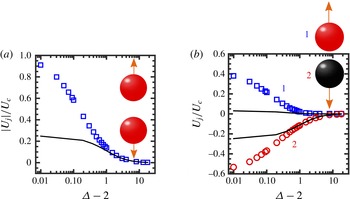
Similarly, a catalytically active colloid with a uniform reaction at its surface can be propelled due to the presence of another active (or passive) colloid. Figure 8(a) represents the non-dimensional velocities (scaled with
 $U_{c}$
) of two catalytically active colloids (
 ${\it\theta}_{cap}^{1}={\it\theta}_{cap}^{2}=180^{\circ }$
) as a function of their separation distance. When the colloids are far from each other, they do not interact as the concentration field is uniform. However, when the separation distance becomes smaller, the presence of the other colloid distorts the concentration field around the first one and it eventually yields a propulsion. Likewise, this scenario would take place for a catalytic colloid (
 ${\it\theta}_{cap}^{1}=180^{\circ }$
) and an inert colloid (
 ${\it\theta}_{cap}^{2}=0^{\circ }$
) which can be considered as a cargo, figure 8(b). Notice the swimming velocities are not equal in magnitude in this case because the solute concentration gradient around the inert particle is stronger compared to the catalytically active particle and hence it translates faster in all separation distances. The solid black lines in figure 8 represent the results found from the method of reflection analysis suggesting the far-field velocity of the catalytic colloids
 ${\sim}1/{\it\Delta}^{5}$
and for the inert one
 ${\sim}1/{\it\Delta}^{2}$
(see appendix C for details). In a similar fashion, it has been recently shown that the symmetry can be also broken not only by taking different chemical activity for two colloids but also by considering two different particle sizes (Michelin & Lauga Reference Michelin and Lauga2015).
3.2.2 Asymmetric motion of two colloidal motors
For arbitrary inclination angles of the colloidal particles, they swim in all three directions and they also undergo solid body rotation. In particular, the motions of colloidal motors are influenced not only by hydrodynamic interactions (problem (b), (d) and (e) in figure 3) but also via diffusive interaction of the solute concentration generated at the active caps of the colloids with the boundary of the other colloid which modifies the propulsive force (problem (a) in figure 3). To disentangle these effects better, we focus on situations where the orientation vectors of the particles
 $\boldsymbol{n}_{p}^{1}$
and
 $\boldsymbol{n}_{p}^{2}$
are in the same plane
 $x$
–
 $z$
and do not have a component in
 $y$
-direction.
As we have observed in the axisymmetric motions, the swimming velocities of colloids depend considerably on their relative orientation, e.g. it does matter in which direction two colloidal motors approach or move away from each other. In order to systematically elucidate this effect, three sets of relative orientations of the colloids are considered. The inclination angles of the colloidal particles are chosen to be complimentary,
 ${\it\Xi}_{1}+{\it\Xi}_{2}=180^{\circ }$
in the first two cases and
 ${\it\Xi}_{1}-{\it\Xi}_{2}=180^{\circ }$
for the third case. In this way, by considering equal surface coverages for the particles, the magnitudes of the swimming translational and angular velocities are identical.
Non-dimensional translational and angular velocities of two Janus colloidal motors (
 ${\it\theta}_{cap}^{1}={\it\theta}_{cap}^{2}=90^{\circ }$
) for three distinct relative orientations as a function of non-dimensional separation distance
 ${\it\Delta}-2$
. The translational non-dimensional velocities in the (a)
 $z$
-direction (parallel to the centre-to-centre line) and (b)
 $x$
-direction (perpendicular to the centre-to-centre line) are non-dimensionalized with the swimming velocity of a Janus colloid at infinite medium
 $U_{\infty }$
and angular velocity (c) around the
 $y$
axis is non-dimensionalized with
 $U_{\infty }/a$
.

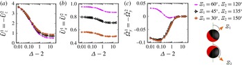
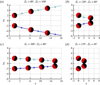
In the first scenario, the active areas of the colloidal motors are on one side and adjacent to each other. Figure 9 illustrates the translational and angular velocities of two Janus colloids as a function of separation distance for three relative orientations. The non-dimensional swimming velocity component, which is along the direction of the centre-to-centre line, approaches the reference value when the colloids are far from each other, i.e.
 $\tilde{U} _{z}^{j}\rightarrow \text{cos}{\it\Xi}_{j}$
, however, for smaller separation distances, this value increases as the concentration of solute becomes larger in the thin gap for all given inclination angles as shown in figure 9(a). The component of non-dimensional swimming velocity in the direction perpendicular to the centre-to-centre line,
 $\tilde{U} _{x}$
, behaves similarly; when the motors are far away from each other, it approaches the reference value
 $\tilde{U} _{x}^{j}\rightarrow \text{sin}{\it\Xi}_{j}$
and when the separation distance is smaller, the colloids translate faster (figure 9
b). This behaviour is predictable based on what was discussed regarding the axisymmetric motions: for smaller separation distances, the solute concentration is strengthened in the thin gap and brings about stronger propulsions. In addition, the hydrodynamic resistance associated with problem (d) in figure 3 becomes weaker as the particles translate in the same direction (see Goldman et al.
Reference Goldman, Cox and Brenner1966) and therefore particles can swim faster. The angular rotation around the
 $y$
axis, on the other hand, is non-monotonic. To explain this trend, we should first determine the sign of the propulsive torques (torques associated with problem (a) in figure 3) on the particles. For the complementary relative orientations given in the first scenario, the propulsive torques on the colloids are always equal and opposite, however, depending on the relative orientations, the signs can be positive (clockwise with respect to the negative
 $y$
axis) or negative (counterclockwise with respect to the negative
 $y$
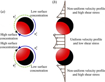
axis). To resolve this complex behaviour, we have to first elucidate the sign of propulsive torques on the particles. The propulsive torques on particles are controlled by the local distribution of the force in the gap which depends on the relative orientations of the colloids and their separation distance. In figure 10(a), the directions of slip velocity
 $\boldsymbol{v}_{s}$
on particle surfaces are schematically shown. In this case, the high surface concentration is along the active caps and the low concentration at the inert sides. The generated surface flow due to solute gradient adjacent to the gap (shown with solid lines) brings about a counterclockwise (clockwise) torque on the particle on top (bottom) while the surface flow on the other section of the particle (shown with dotted lines) yields a clockwise (counterclockwise) torque on the particle on top (bottom). The surface flow along the solid lines are greater in magnitude relative to the dotted lines because the concentration gradient in the gap is stronger and therefore by neglecting the flow generated by the other particle, it is expected the particle on top (bottom) rotates counterclockwise (clockwise) with negative (positive) propulsive torque. However, the local shear stress (velocity gradient) in the gap region can be drastically altered by the interaction of the surface flows generated by the particles. In figure 10(b) the velocity profiles in the gap region and the regions facing opposite to the gaps are schematically demonstrated. As evident from the figure, the velocity profile inside the gap is always more uniform compared to the regions opposite to the gap. This effect can alleviate the local force in the thin gap and reverse the direction of propulsive torques on the particles and hence the competition between these two effects shown in figure 10 at different relative orientations of the particles brings about the complex trend observed in angular velocity (figure 9
c). Furthermore, it is important to note that the resultant hydrodynamic torque due to translational motion of two colloids (figure 3
d) is also involved in determining the angular velocities of the particles however this effect is weaker relative to the propulsive torque in this case.
Schematic representations of (a) the surface flows generated by the solute concentration gradient along the particle surfaces in the first scenario (the dotted and solid lines indicate weak and strong surface flows respectively) and (b) the local velocity profile around the two particles due to their surface flows (phoretic effect).

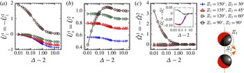
In the second scenario, the passive areas of the colloids are next to each other in an inclined angle and they are both translating in the positive
 $x$
-direction (see figure 11). Figure 11(a) shows the
 $z$
component of the non-dimensional swimming velocity as a function of separation distance for four inclination angles. For three relative inclined orientations, the colloids velocities decrease as the particles swim towards each other and they eventually stops due to the lubrication force in the thin gap. However, for the motion along the positive
 $x$
-direction where
 ${\it\Xi}_{1}={\it\Xi}_{2}=90^{\circ }$
, the non-dimensional swimming velocity in the
 $z$
-direction is amplified by the propulsive force due to the presence of excess solute in the gap between the colloids. The swimming velocity component along
 $x$
and the rotational velocity around
 $y$
for all relative orientations (except the parallel motion (
 ${\it\Xi}_{1}={\it\Xi}_{2}=90^{\circ }$
)) behaves exactly as in the previous case (compare figure 11
b,c with figure 9
b,c). In the case of parallel motion (
 ${\it\Xi}_{1}={\it\Xi}_{2}=90^{\circ }$
), the swimming velocity along the
 $x$
-axis increases initially as the separation distance becomes smaller. However, once the separation distance becomes smaller than
 ${\it\Delta}\sim 2.4$
, the swimming velocity monotonically decreases (see figure 11
b). The rotational velocity around the
 $y$
axis in this case is always positive and it monotonically increases as the colloids approach (open circles in figure 11
c). This complex trend is again due to the coupling of the rotational motion around the
 $y$
axis (positive angular velocity for the colloid on top and negative for the one on the bottom) and positive translational motion in the
 $x$
-direction according to the forces and torques determined from problems (a), (d) and (e) in figure 3.
Non-dimensional translational and angular velocities of two Janus colloidal motors (
 ${\it\theta}_{cap}^{1}={\it\theta}_{cap}^{2}=90^{\circ }$
) for four distinct relative orientations as a function of non-dimensional separation distance
 ${\it\Delta}-2$
. The translational non-dimensional velocities in (a)
 $z$
-direction (parallel to the centre-to-centre line) and (b)
 $x$
-direction (perpendicular to the centre-to-centre line) are non-dimensionalized with the swimming velocity of a Janus colloid at infinite medium
 $U_{\infty }$
and angular velocity (c) around the
 $y$
axis is non-dimensionalized with
 $U_{\infty }/a$
. Inset in (c) demonstrate the non-dimensional angular velocity of the relative orientations with small magnitude of rotation.

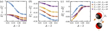
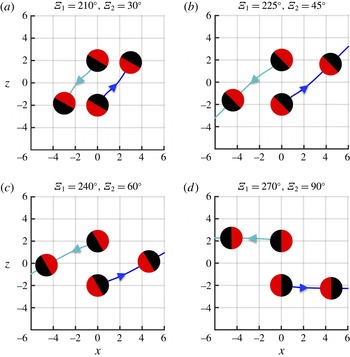
In the third scenario, the active caps face opposite each other in all the given orientations, figure 12. The
 $z$
component of the swimming velocity is identical to the second scenario, figure 12(a). However, the swimming velocity in the
 $x$
-direction and angular velocity behave differently. Figure 12(b) demonstrates the non-dimensional swimming velocity in the
 $x$
-direction as a function of separation distance. The speed of the colloids for all orientations decreases as they move towards each other. To realize the trend in this scenario, we allude again to the hydrodynamic forces associated with problems (d) and (e) in figure 3. For two passive colloidal particles which are translating in opposite directions under a constant force (O’Neill Reference O’Neill1969), the hydrodynamic torques on the two colloids are equal in sign and magnitude and hence the particles rotate in the same direction, e.g. if two passive colloids on the top and bottom of the
 $x$
–
 $y$
plane translate in negative and positive
 $x$
-directions, respectively, the hydrodynamic torque forces both colloids to rotate counterclockwise with respect to the negative
 $y$
-axis. Moreover, the hydrodynamic resistance to the motion of two passive colloids translating in opposite directions along the
 $x$
-axis increases as the separation distance decreases and therefore results in a smaller translational velocity. Figure 12(b) demonstrates the non-dimensional swimming velocity in the
 $x$
-direction as a function of separation distance; the speed of colloids for all of the orientations decreases as they move towards each other since the hydrodynamic resistance scales as
 ${\sim}\text{log}({\it\Delta}-2)$
(Kim & Karrila Reference Kim and Karrila2005). The colloids also rotate faster as they approach each other (see figure 12
c). For the parallel motion (
 ${\it\Xi}_{1}=270^{\circ }$
and
 ${\it\Xi}_{2}=90^{\circ }$
), the rotational velocity is initially positive and then it undergoes a transition to the negative values. The initial positive values are due to the fact that the propulsive torque in this case is always positive, i.e. the torques associated with problem (a) in figure 3 always tend to force the colloids to rotate in such a way that they bring their active sections close to each other and this effect is dominant in the far field once
 ${\it\Xi}_{1}=270^{\circ }$
and
 ${\it\Xi}_{2}=90^{\circ }$
. However, once the colloids approach each other, the hydrodynamic torque associated with problem (d) in figure 3 offsets this positive torque and ultimately compels the colloids to rotate with negative angular velocities.
Non-dimensional translational and angular velocities of two Janus colloidal motors (
 ${\it\theta}_{cap}^{1}={\it\theta}_{cap}^{2}=90^{\circ }$
) for three distinct relative orientations as a function of non-dimensional separation distance
 ${\it\Delta}-2$
. The translational non-dimensional velocities in (a)
 $z$
-direction (parallel to the centre-to-centre line) and (b)
 $x$
-direction (perpendicular to the centre-to-centre line) are non-dimensionalized with the swimming velocity of a Janus colloid at infinite medium
 $U_{\infty }$
and angular velocity (c) around the
 $y$
axis is non-dimensionalized with
 $U_{\infty }/a$
.

3.3 Pair trajectories
To investigate the pair trajectories of colloidal motors, we assume that, similar to previous section, the initial orientation vectors of the motors are both in the
 $x$
–
 $z$
plane and consequently the colloids stay in the same plane for a long time since it was shown that there are no rotations around the
 $z$
and
 $x$
axes and hence the colloids never exit the
 $x$
–
 $z$
plane over a long time period. Generally, for two colloidal particles approaching each other, there are two ultimate possible scenarios: either they (i) interact and ‘escape’ from each other or (ii) they persistently approach and come into contact to assemble. We refer to ‘assembly’ when the non-dimensional separation distance is less than
 ${\it\Delta}<2.01$
. Here, complementary angles for relative orientations are considered, i.e. the initial inclination angles with respect to the line of centres are either
 ${\it\Xi}_{1}+{\it\Xi}_{2}=180^{\circ }$
or
 ${\it\Xi}_{1}-{\it\Xi}_{2}=180^{\circ }$
; the former indicates the conditions where the
 $x$
component of swimming velocities of both motors are in the positive direction while the latter includes situations where the
 $x$
component of swimming velocities are in opposite directions. To obtain particle trajectories, the swimming translational and rotational velocities of the particles were determined initially at each time step in the comoving (Lagrangian) frame and then the particles centre of mass and orientation vectors were updated by explicit integration in time with Euler’s method. The non-dimensional time interval was considered sufficiently small so that the particles do not move (or rotate) considerably in the time interval and the errors due to numerical integration are negligible. For two swimming colloids, the direction of rotation can be altered depending on two parameters: (i) relative orientations and (ii) the active coverages of the colloids.
Pair trajectories of Janus motors for various initial inclination angles where
 ${\it\Xi}_{1}+{\it\Xi}_{2}=180^{\circ }$
.

The relative orientation indicates whether the active sections of the colloidal motors are adjacent or not. If the initial orientation of the motors is set in a fashion similar to the first scenario (see the schematic in figure 9), the build up of the excess concentration of solute in the gap between the particles gives rise to a situation where particles persistently move away from each other until they fail to interact and each one of them swims independently (see figure 13 a).
If the initial relative orientation of the motors is similar to the second scenario, as shown in figure 11, the colloids approach and rotate at the same time until they assemble. For two Janus motors, the directions of rotation at most relative orientations are in a way such that they enhance the assembly process of the particles, i.e. the particles rotate in opposite directions in a way to bring their passive sections aligned and closer. The pair trajectories of two Janus colloids with various initial relative orientations and separation distances of
 ${\it\Delta}=4$
are shown in figure 13(b–d). For initial inclination angles
 ${\it\Xi}_{1}=120^{\circ }$
(figure 13
b) and
 ${\it\Xi}_{1}=100^{\circ }$
(figure 13
c), the particle on top (bottom) rotates clockwise (counterclockwise) with respect to the negative
 $y$
-direction and this in turn enhances the assembly of the particles. For
 ${\it\Xi}_{1}=135^{\circ }$
(figure 13
d), the directions of rotation of the colloids are reversed, however the magnitude of the rotations are too small to allow the particles to escape.
Pair trajectories of Janus motors for various relative initial inclination angles where
 ${\it\Xi}_{1}-{\it\Xi}_{2}=180^{\circ }$
.

In the third scenario, as shown in figure 12, the passive sections of the colloids are adjacent. The typical pair trajectories of two Janus motors for various initial inclination angles
 ${\it\Xi}_{1}$
are illustrated in figure 14. Here, the colloids always rotate in the same direction around the
 $y$
-axis. The particle tend to face their passive sections and for all initial inclination angles
 ${\it\Xi}_{1}>194^{\circ }$
at
 ${\it\Delta}=4$
, the colloids pass each other and escape. For smaller initial inclination angle
 ${\it\Xi}_{1}\leqslant 194^{\circ }$
, the particles block each other’s paths and hence they assemble.
Pair trajectories of catalytically active motors for fixed relative initial inclination angles of
 ${\it\Xi}_{1}={\it\Xi}_{2}=90^{\circ }$
and (a)
 ${\it\theta}_{cap}=90^{\circ }$
, (b)
 ${\it\theta}_{cap}=40^{\circ }$
and (c)
 ${\it\theta}_{cap}=140^{\circ }$
.

In all three scenarios, the active coverages of the colloidal motors play an important role on the pair trajectories. To resolve this fact more clearly, in figure 15 we demonstrate the pair trajectories of active colloidal motors for a fixed relative orientation of
 ${\it\Xi}_{1}={\it\Xi}_{2}=90^{\circ }$
and three different cap angles of
 ${\it\theta}_{cap}^{j}=90^{\circ }$
,
 ${\it\theta}_{cap}^{j}=40^{\circ }$
and
 ${\it\theta}_{cap}^{j}=140^{\circ }$
. In figure 15(a), the pair trajectory of two Janus motors
 ${\it\theta}_{cap}^{j}=90^{\circ }$
is shown; the particles initially move away from each other because the swimming velocity along the
 $z$
-direction is positive (see figure 11
a). However, since the angular velocity around the
 $y$
axis is positive (negative) for the particle on top (bottom) (see figure 11
c), the colloids rotate to bring their passive sections to face the gap and approach in order to assemble. For
 ${\it\theta}_{cap}^{j}=40^{\circ }$
, the directions of rotation of the particles around the
 $y$
axis are reversed (see figure 15
b). This type of pair trajectory is a typical behaviour of two swimming bacteria whose dynamics is usually studied in the context of the squirmer model (Lighthill Reference Lighthill1952; Blake Reference Blake1971; Ishikawa, Simmonds & Pedley Reference Ishikawa, Simmonds and Pedley2006). For larger coverages, the directions of rotation of the particles around the
 $y$
-axis are also reversed. However, the presence of excess solute concentrated in the gap repels the particles to the distant regions where the particles do not interact and therefore swim independently (see figure 15
c). Moreover, for this initial separation distance
 ${\it\Delta}=4$
and inclination angles of
 ${\it\Xi}_{1}={\it\Xi}_{2}=90^{\circ }$
, there is a critical cap angle (coverage)
 ${\it\theta}_{cap}^{1}={\it\theta}_{cap}^{2}=63^{\circ }$
at which the magnitude of the propulsive torque becomes precisely equal in magnitude to the resultant hydrodynamic torques of problem (d) in figure 3 and hence the particles do not rotate. However, this condition is unstable because the swimming velocity component in the
 $z$
-direction is non-zero and hence the particles move away from each other.
Figure 16 shows the pair trajectories that correspond to the third scenario (see figure 12) for three different cap angles. In all cases, the shape of the trajectories are almost similar. However, the direction of rotations are not similar for all coverages. For
 ${\it\theta}_{cap}^{j}=40^{\circ }$
and
 ${\it\theta}_{cap}^{j}=90^{\circ }$
the particles rotate with negative angular velocities since the particles can reach smaller separation distances where the positive propulsive torques (torque associated with problem (a) in figure 3) are small compared to the negative hydrodynamic torques generated by their translational motions in the opposite direction. For high coverage
 ${\it\theta}_{cap}^{j}=140^{\circ }$
on the other hand, the particles are so far that the colloids have positive angular velocities. Moreover, as the particle coverage becomes smaller in size, the particles stay in the sticky lubrication zone much longer and this leads to a more curved pair trajectory (see figure 16
a).
Pair trajectories of catalytically active motors for a fixed relative initial inclination angle
 ${\it\Xi}_{1}=200^{\circ },{\it\Xi}_{2}=20^{\circ }$
and (a)
 ${\it\theta}_{cap}=40^{\circ }$
, (b)
 ${\it\theta}_{cap}=90^{\circ }$
and (c)
 ${\it\theta}_{cap}=140^{\circ }$
. The numbers on (a) are for clarity on particles trajectories.

In the second scenario, particles with very high coverage initially move away to distant regions where they attain positive (particle on top) and negative (particle on bottom) rotations and translate until they reach an axisymmetric orientation, i.e.
 $180^{\circ }$
for the one on top and
 $0^{\circ }$
for the one on bottom, and then approach to assemble (see figure 17
a). Furthermore, the analysis indicates that beyond a critical coverage of
 ${\it\theta}_{cap}=152^{\circ }$
the particles can never be assembled. However, there is one interesting feature in the pair trajectories where the motors become completely stationary (see figure 17
b). At the stationary point, the concentration field around each one of the particles is uniform and hence the propulsive forces/torques are identically zero. Thus they come to a complete stop and then remain stationary indefinitely. This type of trajectory has also been observed for catalytic motors with high coverages in the vicinity of a solid boundary (Uspal et al.
Reference Uspal, Popescu, Dietrich and Tasinkevych2015; Mozaffari et al.
Reference Mozaffari, Sharifi-Mood, Koplik and Maldarelli2016).
Pair trajectories of catalytically active motors for a fixed initial inclination angles of
 ${\it\Xi}_{1}=97^{\circ },{\it\Xi}_{2}=83^{\circ }$
and (a)
 ${\it\theta}_{cap}=140^{\circ }$
(b)
 ${\it\theta}_{cap}=160^{\circ }$
.

4 Conclusions
A combined analytical–numerical solution has been developed to study the pair interaction of catalytically active colloids due to self-diffusiophoresis. These colloids act as ‘motors’ consuming fuel from the immediate environment and create a local concentration gradients of interactive solutes which in turn drive their autonomous motion. Since the driving force for particle propulsion is a solute concentration gradient, we solved for both hydrodynamics and mass transfer equations around two colloidal particles utilizing a continuum approach based on the thin interfacial layer assumption (
 $L\ll a$
) for diffusiophoresis (Anderson Reference Anderson1989). For reaction driven self-diffusiophoresis in non-electrolyte solutions, the interaction length scale
 $L$
depends on the surface interaction being considered, e.g. for a hard-sphere excluded volume interaction,
 $L$
is of the characteristic size of the molecule which would typically be in the range of 1–10 nm. The analysis depicted here was performed employing two important assumptions: firstly, the entire analysis of two colloidal microparticles (
 $a\sim 1~{\rm\mu}\text{m}$
) based on the thin interfacial assumption is valid until that particle minimum separation distance
 $d-2a$
is nanometric and comparable to the surface roughness; below this limit (
 $d-2a<10~\text{nm}$
) we assume the particles are almost in contact and hence we use the term assembly. Furthermore, in the limits of
 $Da\ll 1$
and
 $Pe\ll 1$
the governing equations of the solute mass transfer is decoupled from the hydrodynamics. Considering nanometric-sized solutes and micron-sized motors, these two assumptions remains valid until the gap region between the particle becomes comparable to the solute size
 $d-2a\sim a_{s}\sim 10^{-9}~\text{m}$
. Having utilized these assumptions, the mass transfer problem was solved exactly in bispherical coordinates. For the hydrodynamics, we took advantage of the Reynolds reciprocal theorem to write the propulsive forces and torques on the colloids as quadratures.
The results presented here show that the dynamics and trajectories of two catalytically active colloids are much richer and more complex than other self-propelled particles that solely interact via hydrodynamics, i.e. colloidal squirmers. For catalytic particles, the presence of a second particle distorts the solute concentration around the first particle and therefore modifies its propulsive force and torque. Thus, employing purely hydrodynamic models with a constant force or source dipoles fails to capture the actual dynamics of catalytically driven active colloids. As evident in these systems, the local concentration gradient of solutes can push (or pull) the colloids from the domains with high solute concentration resulting in depleted (or aggregated) zones. The hydrodynamic interaction is the second effect which influences the dynamics and particle trajectories. In conclusion, the dynamics at the pair level is controlled by the active coverage of catalytic caps
 ${\it\theta}_{cap}^{j}$
and the relative orientation of the colloids
 ${\it\Xi}_{j}$
, (
 $j=1$
and 2).
When the active areas of the colloids are aligned, the motions are axisymmetric and particles do not rotate. For situations where active surfaces are adjacent, the solute concentration rises in the gap between the colloids, which causes them to experience an increase in propulsive force. By contrast, when the passive surfaces of the particles are adjacent, the propulsive forces do not changes significantly while particles are approaching each other and therefore their swimming velocities are reduced by lubrication forces.
When the active areas of the colloids are not aligned completely, the motions are asymmetric and the colloids rotate and translate at the same time. For situations where the orientation vectors of the colloidal motors are in the
 $x$
–
 $z$
plane (see figure 2), there are two possible scenarios for the particles: colloids can either swim towards each other and come into contact (assembly) or they can move away from each other (escape). Note that the criteria for assembly of the particles are considered when the non-dimensional centre-to-centre separation distance
 ${\it\Delta}$
is less than 2.01. The direction of colloids rotations determine which one of the two scenarios takes place. Based on the predictions of this model, a phase diagram is sketched in figure 18 for the long-time behaviour of two non-Brownian particles with similar coverage
 ${\it\theta}_{cap}$
at an initial separation distance of
 ${\it\Delta}=4$
and complementary relative orientations of
 ${\it\Xi}_{1}+{\it\Xi}_{2}=180^{\circ }$
(figure 18
a) and
 ${\it\Xi}_{1}-{\it\Xi}_{2}=180^{\circ }$
(figure 18(b)). For small coverages, there are a greater range of angles of initial relative orientation of the particles for which they come into contact, while for larger coverage, the condition of assembly occurs under more stringent conditions and beyond a critical coverage of
 ${\it\theta}_{cap}=152^{\circ }$
the particles never come into contact. We believe this phase diagram has important implications on the elucidation of the clustering and phase separation of catalytically self-propelled particles from a mechanical perspective and could be useful for experimentalists.
Phase diagrams of pair trajectories of catalytically active colloids with identical coverage
 ${\it\theta}_{cap}$
and initial separation distance of
 ${\it\Delta}=4$
for complementary angles of (a)
 ${\it\Xi}_{1}+{\it\Xi}_{2}=180^{\circ }$
and (b)
 ${\it\Xi}_{1}-{\it\Xi}_{2}=180^{\circ }$
.

While the solution presented here is valid at arbitrary particle separation distances, similar analysis can be readily undertaken for the small gap region where
 $L\ll d-2a\ll a$
, in this case the diffusion equation should be solved in the tangent sphere coordinates similar to other problems discussed in the literature in the context of electrophoresis (Yariv & Brenner Reference Yariv and Brenner2003) and potential flow (Jeffrey & Chen Reference Jeffrey and Chen1977). On the other hand, one can still take advantage of RRT for hydrodynamics but the stress tensor associated with the test problems in RRT should be replaced with the relevant near-field solutions of two spheres in the Stokes flow regime (Cooley & O’Neill Reference Cooley and O’Neill1969; O’Neill & Majumdar Reference O’Neill and Majumdar1970b
).
Finally, the pair level analysis we undertook in the present study can be a basis for pursuing much more complex systems in understanding the hydrodynamics of active matter. In particular, a suspension of catalytically active particles has a unique feature in which the active particles can chemically signal each other and be pulled (or pushed) to the certain regions in the system. However, a detailed and quantitative analysis of the collective behaviour of catalytically driven active particles requires taking into account two formidable challenges: (i) the many-body hydrodynamic and phoretic interactions and (ii) Brownian motion. This can be accomplished by employing Stokesian dynamics simulations (Brady & Bossis Reference Brady and Bossis1988) which we will address in a future communication.
Acknowledgement
N.S.-M. thanks N. Bade for proofreading the paper and helpful discussions. U.M.C.-F. is supported by National Science Foundation grants CBET – 1055284 and EPS – 1010674.
Appendix A. Recursive relations for the concentration field around two colloids
In this section, we provide the recursive relationships found by applying the boundary conditions on particle surfaces for the concentration field,
 $$\begin{eqnarray}\displaystyle & & \displaystyle -\left[n\sinh (n-0.5){\it\beta}_{j}\right]\tilde{A}_{n-1,0}+\left[\sinh {\it\beta}_{j}\cosh (n+0.5){\it\beta}_{j}\right.\nonumber\\ \displaystyle & & \displaystyle \quad \left.+\,(2n+1)\cosh {\it\beta}_{j}\sinh (n+0.5){\it\beta}_{j}\right]\tilde{A}_{n,0}-\left[(n+1)\sinh (n+1.5){\it\beta}_{j}\right]\tilde{A}_{n+1,0}\nonumber\\ \displaystyle & & \displaystyle \quad -\left[n\cosh (n-0.5){\it\beta}_{j}\right]\tilde{B}_{n-1,0}+\left[\sinh {\it\beta}_{j}\sinh (n+0.5){\it\beta}_{j}\right.\nonumber\\ \displaystyle & & \displaystyle \quad \left.+\,(2n+1)\cosh {\it\beta}_{j}\cosh (n+0.5){\it\beta}_{j}\right]\tilde{B}_{n,0}-\left[(n+1)\cosh (n+1.5){\it\beta}_{j}\right]\tilde{B}_{n+1,0}\nonumber\\ \displaystyle & & \displaystyle \quad ={\it\Psi}_{n,0}^{j},\end{eqnarray}$$
 $$\begin{eqnarray}\displaystyle & & \displaystyle -\left[(n-m)\sinh (n-0.5){\it\beta}_{j}\right]\tilde{A}_{n-1,m}+\left[\sinh {\it\beta}_{j}\cosh (n+0.5){\it\beta}_{j}\right.\nonumber\\ \displaystyle & & \displaystyle \quad \left.+\,(2n+1)\cosh {\it\beta}_{j}\sinh (n+0.5){\it\beta}_{j}\right]\tilde{A}_{n,m}-\left[(n+m+1)\sinh (n+1.5){\it\beta}_{j}\right]\tilde{A}_{n+1,m}\nonumber\\ \displaystyle & & \displaystyle \quad -\,\left[(n-m)\cosh (n-0.5){\it\beta}_{j}\right]\tilde{B}_{n-1,m}+\left[\sinh {\it\beta}_{j}\sinh (n+0.5){\it\beta}_{j}\right.\nonumber\\ \displaystyle & & \displaystyle \quad \left.+\,(2n+1)\cosh {\it\beta}_{j}\cosh (n+0.5){\it\beta}_{j}\right]\tilde{B}_{n,m}-\left[(n+m+1)\cosh (n+1.5){\it\beta}_{j}\right]\tilde{B}_{n+1,m}\nonumber\\ \displaystyle & & \displaystyle \quad ={\it\Psi}_{n,m}^{j},\end{eqnarray}$$
 $$\begin{eqnarray}\displaystyle & & \displaystyle -\left[(n-m)\sinh (n-0.5){\it\beta}_{j}\right]\tilde{C}_{n-1,m}+\left[\sinh {\it\beta}_{j}\cosh (n+0.5){\it\beta}_{j}\right.\nonumber\\ \displaystyle & & \displaystyle \quad \left.+\,(2n+1)\cosh {\it\beta}_{j}\sinh (n+0.5){\it\beta}_{j}\right]\tilde{C}_{n,m}-\left[(n+m+1)\sinh (n+1.5){\it\beta}_{j}\right]\tilde{C}_{n+1,m}\nonumber\\ \displaystyle & & \displaystyle \quad -\,\left[(n-m)\cosh (n-0.5){\it\beta}_{j}\right]\tilde{D}_{n-1,m}+\left[\sinh {\it\beta}_{j}\sinh (n+0.5){\it\beta}_{j}\right.\nonumber\\ \displaystyle & & \displaystyle \quad \left.+\,(2n+1)\cosh {\it\beta}_{j}\cosh (n+0.5){\it\beta}_{j}\right]\tilde{D}_{n,m}-\left[(n+m+1)\cosh (n+1.5){\it\beta}_{j}\right]\tilde{D}_{n+1,m}\nonumber\\ \displaystyle & & \displaystyle \quad =\text{Z}_{n,m}^{j},\end{eqnarray}$$
where we have
 $$\begin{eqnarray}\displaystyle & \displaystyle {\it\Psi}_{n,0}^{j}=\frac{2n+1}{4{\rm\pi}}\int _{0}^{2{\rm\pi}}\text{d}{\it\phi}\int _{0}^{{\rm\pi}}\frac{2c{\it\vartheta}_{j}u_{j}}{\sqrt{\cosh {\it\beta}_{j}-\cos {\it\alpha}}}\sin {\it\alpha}P_{n}^{0}(\cos {\it\alpha})\,\text{d}{\it\alpha}, & \displaystyle\end{eqnarray}$$
 $$\begin{eqnarray}\displaystyle & \displaystyle {\it\Psi}_{n,m}^{j}=\frac{(2n+1)(n-m)!}{2{\rm\pi}(n+m)!}\int _{0}^{2{\rm\pi}}\text{d}{\it\phi}\int _{0}^{{\rm\pi}}\frac{2c{\it\vartheta}_{j}u_{j}\cos m{\it\phi}}{\sqrt{\cosh {\it\beta}_{j}-\cos {\it\alpha}}}\sin {\it\alpha}P_{n}^{m}(\cos {\it\alpha})\,\text{d}{\it\alpha}, & \displaystyle\end{eqnarray}$$
 $$\begin{eqnarray}\displaystyle & \displaystyle \text{Z}_{n,m}^{j}=\frac{(2n+1)(n-m)!}{2{\rm\pi}(n+m)!}\int _{0}^{2{\rm\pi}}\text{d}{\it\phi}\int _{0}^{{\rm\pi}}\frac{2c{\it\vartheta}_{j}u_{j}\sin m{\it\phi}}{\sqrt{\cosh {\it\beta}_{j}-\cos {\it\alpha}}}\sin {\it\alpha}P_{n}^{m}(\cos {\it\alpha})\,\text{d}{\it\alpha}. & \displaystyle\end{eqnarray}$$
Note that each one of (A 1)–(A 3) is the two equations for
 $j=1$
and
 $2$
.
Appendix B. Stokes flow solution of two identical spherical colloids
In this section we provide the detailed solution of Stokes flow around two identical colloids. For arbitrary motion of the colloids, the motion can be described as translational motions parallel and perpendicular to the centre-to-centre lines and rotational motion around the third axis. To calculate the hydrodynamic forces and torques on colloids and utilizing Reynolds reciprocal theorem (RRT), we recapitulate the hydrodynamic solutions in this section. The Stokes flow solution of the velocity field in cylindrical coordinates
 $({\it\rho},{\it\phi},z)$
in the form of eigensolutions of bispherical coordinates is given by
 $$\begin{eqnarray}\displaystyle p({\it\alpha},{\it\beta},{\it\phi}) & = & \displaystyle \frac{\sqrt{\cosh {\it\beta}-\cos {\it\alpha}}}{c}\mathop{\sum }_{n=1}^{\infty }\left(A_{n}\sinh \left(n+\frac{1}{2}\right){\it\beta}+B_{n}\cosh \left(n+\frac{1}{2}\right){\it\beta}\right)\nonumber\\ \displaystyle & & \displaystyle P_{n}^{1}(\cos {\it\alpha})\cos {\it\phi},\end{eqnarray}$$
 $$\begin{eqnarray}\displaystyle v_{{\it\rho}} & = & \displaystyle \frac{\sin {\it\alpha}}{2\sqrt{\cosh {\it\beta}-\cos {\it\alpha}}}\mathop{\sum }_{n=1}^{\infty }\!\left(\!A_{n}\sinh \!\left(\!n+\frac{1}{2}\right)\!{\it\beta}+B_{n}\cosh \!\left(\!n+\frac{1}{2}\!\right){\it\beta}\right)P_{n}^{1}(\cos {\it\alpha})\;\cos {\it\phi}\nonumber\\ \displaystyle & & \displaystyle +\,\frac{\sqrt{\cosh {\it\beta}-\cos {\it\alpha}}}{2}\!\left[\mathop{\sum }_{n=2}^{\infty }\!\left(\!E_{n}\sinh \!\left(\!n+\frac{1}{2}\!\right)\!{\it\beta}+F_{n}\cosh \!\left(\!n+\frac{1}{2}\!\right)\!{\it\beta}\!\right)P_{n}^{2}(\cos {\it\alpha})\cos {\it\phi}\right.\nonumber\\ \displaystyle & & \displaystyle \left.+\mathop{\sum }_{n=0}^{\infty }\left(G_{n}\sinh \left(n+\frac{1}{2}\right){\it\beta}+H_{n}\cosh \left(n+\frac{1}{2}\right){\it\beta}\right)\;P_{n}^{0}(\cos {\it\alpha})\;\cos {\it\phi}\right],\end{eqnarray}$$
 $$\begin{eqnarray}\displaystyle v_{{\it\phi}} & = & \displaystyle \frac{\sqrt{\cosh {\it\beta}-\cos {\it\alpha}}}{2}\!\left[\mathop{\sum }_{n=2}^{\infty }\!\left(\!E_{n}\sinh \left(n+\frac{1}{2}\right)\!{\it\beta}+F_{n}\cosh \left(\!n+\frac{1}{2}\right)\!{\it\beta}\!\right)P_{n}^{2}(\cos {\it\alpha})\sin {\it\phi}\right.\nonumber\\ \displaystyle & & \displaystyle \left.-\mathop{\sum }_{n=0}^{\infty }\left(G_{n}\sinh \left(n+\frac{1}{2}\right){\it\beta}+H_{n}\cosh \left(n+\frac{1}{2}\right){\it\beta}\right)P_{n}^{0}(\cos {\it\alpha})\sin {\it\phi}\right],\end{eqnarray}$$
 $$\begin{eqnarray}\displaystyle v_{z} & = & \displaystyle \frac{\sinh {\it\beta}}{2\sqrt{\cosh {\it\beta}-\cos {\it\alpha}}}\mathop{\sum }_{n=1}^{\infty }\left(\!A_{n}\sinh \!\left(n+\frac{1}{2}\right){\it\beta}+B_{n}\cosh \!\left(\!n+\frac{1}{2}\right)\!{\it\beta}\!\right)P_{n}^{1}(\cos {\it\alpha})\cos {\it\phi}\nonumber\\ \displaystyle & & \displaystyle +\,\sqrt{\cosh {\it\beta}-\cos {\it\alpha}}\mathop{\sum }_{n=1}^{\infty }\!\left(\!C_{n}\sinh \!\left(\!n+\frac{1}{2}\right)\!{\it\beta}+D_{n}\cosh \!\left(\!n+\frac{1}{2}\right)\!{\it\beta}\!\right)P_{n}^{1}(\cos {\it\alpha})\cos {\it\phi},\nonumber\\ \displaystyle & & \displaystyle\end{eqnarray}$$
where 8 sets of unknown coefficients, namely
 $A_{n}$
,
 $B_{n},\ldots ,H_{n}$
, have to be obtained from satisfying the boundary conditions at the surface of the two particles and also the equation of continuity.
To study the translational and rotational motions perpendicular to the line of centres and around the third axis, we have to find the following four solutions.
B.1 Slow translation of two identical spheres with similar velocities in magnitude and directions along the direction perpendicular to their line of centres
The slow translation of two non-rotating identical spheres where the two particles are moving in the same direction and with the same velocity
 $U_{\bot }^{1}$
perpendicular to their line of centres is considered here. Boundary conditions at the surface of two particles are equivalent and are given by:
 $$\begin{eqnarray}\displaystyle \left.\begin{array}{@{}c@{}}\left.v_{{\it\rho}}\right|_{{\it\beta}={\it\beta}_{1}}=U_{\bot }^{1}\;\cos {\it\phi},\\ \left.v_{{\it\phi}}\right|_{{\it\beta}={\it\beta}_{1}}=-U_{\bot }^{1}\;\sin {\it\phi},\\ \left.v_{z}\right|_{{\it\beta}={\it\beta}_{1}}=0.\end{array}\right\} & & \displaystyle\end{eqnarray}$$
In the above equations,
 ${\it\beta}={\it\beta}_{1}$
represents the surface of a spherical particle and if
 ${\it\beta}_{1}$
is positive it is located above the
 $x$
–
 $y$
plane. It can be easily shown that the only non-zero coefficients are
 $B_{n}$
,
 $C_{n}$
,
 $F_{n}$
and
 $H_{n}$
and, using boundary conditions given in (B 5), this yields the following recursive relations among these four coefficients
 $$\begin{eqnarray}\displaystyle & & \displaystyle \displaystyle -\frac{1}{2(2n-1)}\cosh \left(n-\frac{1}{2}\right){\it\beta}_{1}\;B_{n-1}+\frac{1}{2(2n+3)}\cosh \left(n+\frac{3}{2}\right){\it\beta}_{1}\;B_{n+1}\nonumber\\ \displaystyle & & \displaystyle \quad \displaystyle -\,\frac{(n-2)}{(2n-1)}\cosh \left(n-\frac{1}{2}\right){\it\beta}_{1}\;F_{n-1}+\cosh {\it\beta}_{1}\cosh \left(n+\frac{1}{2}\right){\it\beta}_{1}\;F_{n}\nonumber\\ \displaystyle & & \displaystyle \quad \displaystyle -\,\frac{(n+3)}{(2n+3)}\;\cosh \left(n+\frac{3}{2}\right){\it\beta}_{1}\;F_{n+1}=0,\end{eqnarray}$$
 $$\begin{eqnarray}\displaystyle & & \displaystyle \displaystyle \frac{(n-1)\;n}{2(2n-1)}\cosh \left(n-\frac{1}{2}\right){\it\beta}_{1}\;B_{n-1}-\frac{(n+1)(n+2)}{2(2n+3)}\cosh \left(n+\frac{3}{2}\right){\it\beta}_{1}\;B_{n+1}\nonumber\\ \displaystyle & & \displaystyle \quad \displaystyle -\,\frac{n}{(2n-1)}\cosh \left(n-\frac{1}{2}\right){\it\beta}_{1}H_{n-1}+\cosh {\it\beta}_{1}\cosh \left(n+\frac{1}{2}\right){\it\beta}_{1}\;H_{n}\nonumber\\ \displaystyle & & \displaystyle \quad \displaystyle -\,\frac{(n+1)}{(2n+3)}\cosh \left(n+\frac{3}{2}\right){\it\beta}_{1}\;H_{n+1}=2\sqrt{2}\nonumber\\ \displaystyle & & \displaystyle \quad \times \,\left[\cosh {\it\beta}_{1}\;\text{e}^{-(n+1/2){\it\beta}_{1}}-\left(\frac{n}{2n-1}\right)\text{e}^{-(n-1/2){\it\beta}_{1}}-\left(\frac{n+1}{2n+3}\right)\text{e}^{-(n+3/2){\it\beta}_{1}}\right],\end{eqnarray}$$
 $$\begin{eqnarray}\displaystyle & & \displaystyle \frac{\sinh {\it\beta}_{1}}{2}\;\cosh \left(n+\frac{1}{2}\right){\it\beta}_{1}\;B_{n}-\frac{(n-1)}{(2n-1)}\sinh \left(n-\frac{1}{2}\right){\it\beta}_{1}\;C_{n-1}\nonumber\\ \displaystyle & & \displaystyle \qquad \quad +\,\cosh {\it\beta}_{1}\sinh \left(n+\frac{1}{2}\right){\it\beta}_{1}\;C_{n}-\frac{(n+2)}{(2n+3)}\sinh \left(n+\frac{3}{2}\right){\it\beta}_{1}\;C_{n+1}=0.\qquad\end{eqnarray}$$
Finally the velocity components should satisfy the equation of continuity,
 $$\begin{eqnarray}\displaystyle & & \displaystyle {\textstyle \frac{-1}{2}}(n-1)\;B_{n-1}+{\textstyle \frac{5}{2}}\;B_{n}+{\textstyle \frac{1}{2}}(n+2)\;B_{n+1}-(n-1)\;C_{n-1}\nonumber\\ \displaystyle & & \displaystyle +\,(2n+1)C_{n}-(n+2)C_{n+1}-{\textstyle \frac{1}{2}}(n-2)(n-1)F_{n-1}+(n+2)(n-1)F_{n}\nonumber\\ \displaystyle & & \displaystyle -\,{\textstyle \frac{1}{2}}(n+2)(n+3)F_{n+1}+{\textstyle \frac{1}{2}}H_{n-1}-H_{n}+{\textstyle \frac{1}{2}}H_{n+1}=0.\end{eqnarray}$$
Equation (B 6) is valid for
 $n\geqslant 2$
, (B 7) for
 $n\geqslant 0$
and (B 8)–(B 9) for
 $n\geqslant 1$
. Four sets of unknown coefficients are obtained from simultaneous solution of the above equations and, as the particle separation distances becomes smaller, more terms in the series should be kept to reach an accurate result. The hydrodynamic forces on the colloids are equal in magnitude and sign, however, the torques are equal in magnitude but opposite in signs:
 $$\begin{eqnarray}\displaystyle & \displaystyle \mathscr{F}_{\bot }^{j,1}=-2\sqrt{2\;}{\rm\pi}\;\sinh {\it\beta}_{1}\;{\it\mu}\;U_{\bot }^{1}\,a\;\mathop{\sum }_{n=0}^{\infty }H_{n}, & \displaystyle\end{eqnarray}$$
 $$\begin{eqnarray}\displaystyle & \displaystyle \mathscr{T}_{\otimes }^{j,1}=\pm 2\sqrt{2\;}{\rm\pi}\;\left(\sinh {\it\beta}_{1}\right)^{2}\;{\it\mu}\;U_{\bot }^{1}\,a^{2}\;\mathop{\sum }_{n=0}^{\infty }\left(2n+1-\coth {\it\beta}_{1}\right)H_{n}, & \displaystyle\end{eqnarray}$$
 $j=1$
or
 $2$
refers to the colloid at positive and negative
 $z$
, respectively.
B.2 Slow rotation of two identical spheres about an axis perpendicular to their line of centres and in opposite directions
In this section, we solve the equations of motion and continuity for two identical non-translating spheres that are rotating around the third axis which passes through their centre and normal to their line of centres with equal angular velocity
 ${\it\Omega}_{\otimes }^{2}$
but in the opposite directions. The relevant boundary conditions at the surface of first sphere are given by
 $$\begin{eqnarray}\displaystyle \left.\begin{array}{@{}c@{}}\left.v_{{\it\rho}}\right|_{{\it\beta}={\it\beta}_{1}}={\it\Omega}_{\otimes }^{2}\left(z-{\it\Delta}/2\right)\cos {\it\phi},\\ \left.v_{{\it\phi}}\right|_{{\it\beta}={\it\beta}_{1}}=-{\it\Omega}_{\otimes }^{2}\left(z-{\it\Delta}/2\right)\sin {\it\phi},\\ \left.v_{z}\right|_{{\it\beta}={\it\beta}_{1}}=-{\it\Omega}_{\otimes }^{2}\;{\it\rho}\cos {\it\phi},\end{array}\right\} & & \displaystyle\end{eqnarray}$$
and the boundary conditions at the surface of the second sphere are
 $$\begin{eqnarray}\displaystyle \left.\begin{array}{@{}c@{}}\left.v_{{\it\rho}}\right|_{{\it\beta}=-{\it\beta}_{1}}=-{\it\Omega}_{\otimes }^{2}\left(z+{\it\Delta}/2\right)\cos {\it\phi},\\ \left.v_{{\it\phi}}\right|_{{\it\beta}=-{\it\beta}_{1}}={\it\Omega}_{\otimes }^{2}\left(z+{\it\Delta}/2\right)\sin {\it\phi},\\ \left.v_{z}\right|_{{\it\beta}=-{\it\beta}_{1}}={\it\Omega}_{\otimes }^{2}\;{\it\rho}\cos {\it\phi}.\end{array}\right\} & & \displaystyle\end{eqnarray}$$
Applying conditions (B 12)–(B 13) in cylindrical components of equations of motion, (B 2)–(B 4), it turns out that the only non-vanishing coefficients are
 $B_{n}$
,
 $C_{n}$
,
 $F_{n}$
and
 $H_{n}$
. Four relationships are needed to obtain this set of four unknown coefficients and it can be readily shown that two following recursive relationships along with (B 6) and (B 9) solves the problem:
 $$\begin{eqnarray}\displaystyle & & \displaystyle \hspace{-30.0pt}\frac{(n-1)\;n}{2(2n-1)}\cosh \left(n-\frac{1}{2}\right){\it\beta}_{1}\;B_{n-1}-\frac{(n+1)(n+2)}{2(2n+3)}\cosh \left(n+\frac{3}{2}\right){\it\beta}_{1}\;B_{n+1}\nonumber\\ \displaystyle & & \displaystyle \hspace{-30.0pt}\qquad -\,\frac{n}{(2n-1)}\cosh \left(n-\frac{1}{2}\right){\it\beta}_{1}H_{n-1}+\cosh {\it\beta}_{1}\cosh \left(n+\frac{1}{2}\right){\it\beta}_{1}\;H_{n}\nonumber\\ \displaystyle & & \displaystyle \hspace{-30.0pt}\qquad -\,\frac{(n+1)}{(2n+3)}\cosh \left(n+\frac{3}{2}\right){\it\beta}_{1}\;H_{n+1}=2\sqrt{2}\;c\left[-\frac{1}{\sinh {\it\beta}_{1}}\;\text{e}^{-(n+1/2){\it\beta}_{1}}\right.\nonumber\\ \displaystyle & & \displaystyle \hspace{-30.0pt}\qquad \left.+\,\coth {\it\beta}_{1}\left(\!\frac{n}{2n-1}\right)\text{e}^{-(n-1/2){\it\beta}_{1}}+\coth {\it\beta}_{1}\left(\frac{n+1}{2n+3}\!\right)\text{e}^{-(n+3/2){\it\beta}_{1}}\right]\!,\quad (n\geqslant 0),\end{eqnarray}$$
 $$\begin{eqnarray}\displaystyle & & \displaystyle \hspace{-30.0pt}\frac{\sinh {\it\beta}_{1}}{2}\;\cosh \left(n+\frac{1}{2}\right){\it\beta}_{1}B_{n}-\frac{(n-1)}{(2n-1)}\sinh \left(n-\frac{1}{2}\right){\it\beta}_{1}C_{n-1}\nonumber\\ \displaystyle & & \displaystyle \hspace{-30.0pt}\qquad +\,\cosh {\it\beta}_{1}\sinh \left(n+\frac{1}{2}\right){\it\beta}_{1}\;C_{n}-\frac{(n+2)}{(2n+3)}\sinh \left(n+\frac{3}{2}\right){\it\beta}_{1}\;C_{n+1}\nonumber\\ \displaystyle & & \displaystyle \hspace{-30.0pt}\quad =-\sqrt{2}\;c\;\left[\left(\frac{-1}{2n-1}\right)\text{e}^{-(n-1/2){\it\beta}_{1}}+\left(\frac{1}{2n+3}\right)\text{e}^{-(n+3/2){\it\beta}_{1}}\right],\quad (n\geqslant 1).\end{eqnarray}$$
The hydrodynamic forces on the colloids are similar in magnitude and sign however, the torques are equal in magnitude but opposite in sign:
 $$\begin{eqnarray}\displaystyle & \displaystyle \mathscr{F}_{\bot }^{j,2}=2\sqrt{2\;}{\rm\pi}\;\sinh {\it\beta}_{1}\;{\it\mu}\;{\it\Omega}_{\otimes }^{2}\,a^{2}\;\mathop{\sum }_{n=0}^{\infty }H_{n}, & \displaystyle\end{eqnarray}$$
 $$\begin{eqnarray}\displaystyle & \displaystyle \mathscr{T}_{\otimes }^{j,2}=\mp 2\sqrt{2\;}{\rm\pi}\;\left(\sinh {\it\beta}_{1}\right)^{2}\;{\it\mu}\;{\it\Omega}_{\otimes }^{2}\,a^{3}\;\mathop{\sum }_{n=0}^{\infty }\left(2n+1-\coth {\it\beta}_{1}\right)H_{n}, & \displaystyle\end{eqnarray}$$
 $j=1$
or
 $2$
refers to the colloid at positive and negative
 $z$
, respectively.
B.3 Slow translation of two identical spheres with similar velocities in magnitude but opposite directions along the direction perpendicular to their line of centres
In this problem, one sphere is translating without rotation with velocity
 $U_{\bot }^{3}$
towards the positive direction normal to the line of centres while the other identical sphere moves with the velocity
 $-U_{\bot }^{3}$
towards the negative direction or vice versa. The boundary conditions at each point on the surface of a sphere whose centre is located at
 $z>0$
can be expressed as
 $$\begin{eqnarray}\displaystyle \left.\begin{array}{@{}c@{}}\displaystyle \left.v_{{\it\rho}}\right|_{{\it\beta}={\it\beta}_{1}}=U_{\bot }^{3}\;\cos {\it\phi},\\ \displaystyle \left.v_{{\it\phi}}\right|_{{\it\beta}={\it\beta}_{1}}=-U_{\bot }^{3}\;\sin {\it\phi},\\ \displaystyle \left.v_{z}\right|_{{\it\beta}={\it\beta}_{1}}=0.\end{array}\right\} & & \displaystyle\end{eqnarray}$$
For the sphere whose centre is located at a negative value of
 $z$
, the related boundary conditions for this non-rotating sphere is given by
 $$\begin{eqnarray}\displaystyle \left.\begin{array}{@{}c@{}}\displaystyle \left.v_{{\it\rho}}\right|_{{\it\beta}=-{\it\beta}_{1}}=-U_{\bot }^{3}\;\cos {\it\phi},\\ \displaystyle \left.v_{{\it\phi}}\right|_{{\it\beta}=-{\it\beta}_{1}}=U_{\bot }^{3}\;\sin {\it\phi},\\ \displaystyle \left.v_{z}\right|_{{\it\beta}=-{\it\beta}_{1}}=0.\end{array}\right\} & & \displaystyle\end{eqnarray}$$
It can be immediately shown that coefficients
 $B_{n}$
,
 $C_{n}$
,
 $F_{n}$
and
 $H_{n}$
in the general solution of the Stokes flow, (B 2)–(B 4), are zero. In order to find the remaining coefficients, the following sets of relations (which can be determined by satisfying appropriate boundary conditions at the particle surfaces as well as the equation of continuity) have to be solved simultaneously:
 $$\begin{eqnarray}\displaystyle & \displaystyle -\frac{1}{2(2n-1)}\sinh \left(n-\frac{1}{2}\right){\it\beta}_{1}\;A_{n-1}+\frac{1}{2(2n+3)}\sinh \left(n+\frac{3}{2}\right){\it\beta}_{1}\;A_{n+1} & \displaystyle \nonumber\\ \displaystyle & \displaystyle -\frac{(n-2)}{(2n-1)}\sinh \left(n-\frac{1}{2}\right){\it\beta}_{1}\;E_{n-1}+\cosh {\it\beta}_{1}\sinh \left(n+\frac{1}{2}\right){\it\beta}_{1}\;E_{n} & \displaystyle \nonumber\\ \displaystyle & \displaystyle -\frac{(n+3)}{(2n+3)}\;\sinh \left(n+\frac{3}{2}\right){\it\beta}_{1}\;E_{n+1}=0,\quad (n\geqslant 2), & \displaystyle\end{eqnarray}$$
 $$\begin{eqnarray}\displaystyle & & \displaystyle \frac{(n-1)\;n}{2(2n-1)}\sinh \left(n-\frac{1}{2}\right){\it\beta}_{1}\;A_{n-1}-\frac{(n+1)(n+2)}{2(2n+3)}\sinh \left(n+\frac{3}{2}\right){\it\beta}_{1}\;A_{n+1}\nonumber\\ \displaystyle & & \displaystyle \quad -\frac{n}{(2n-1)}\sinh \left(n-\frac{1}{2}\right){\it\beta}_{1}G_{n-1}+\cosh {\it\beta}_{1}\sinh \left(n+\frac{1}{2}\right){\it\beta}_{1}\;G_{n}\nonumber\\ \displaystyle & & \displaystyle \quad -\frac{(n+1)}{(2n+3)}\sinh \left(n+\frac{3}{2}\right){\it\beta}_{1}\;G_{n+1}=2\sqrt{2}\;\left[\vphantom{\left(\frac{n}{2n-1}\right)}\cosh {\it\beta}_{1}\;\text{e}^{-(n+1/2){\it\beta}_{1}}\right.\nonumber\\ \displaystyle & & \displaystyle \quad \left.-\left(\frac{n}{2n-1}\right)\text{e}^{-(n-1/2){\it\beta}_{1}}-\left(\frac{n+1}{2n+3}\right)\text{e}^{-(n+3/2){\it\beta}_{1}}\right],\quad (n\geqslant 0),\end{eqnarray}$$
 $$\begin{eqnarray}\displaystyle & & \displaystyle \hspace{-14.39996pt}\frac{\sinh {\it\beta}_{1}}{2}\;\sinh \left(n+\frac{1}{2}\right){\it\beta}_{1}A_{n}-\frac{(n-1)}{(2n-1)}\cosh \left(n-\frac{1}{2}\right){\it\beta}_{1}D_{n-1}\nonumber\\ \displaystyle & & \displaystyle \hspace{-14.39996pt}\quad +\,\cosh {\it\beta}_{1}\cosh \!\left(\!n+\frac{1}{2}\right)\!{\it\beta}_{1}D_{n}-\frac{(n+2)}{(2n+3)}\cosh \!\left(\!n+\frac{3}{2}\right){\it\beta}_{1}D_{n+1}=0,\quad (n\geqslant 1),\qquad\end{eqnarray}$$
 $$\begin{eqnarray}\displaystyle & & \displaystyle {\textstyle \frac{-1}{2}}(n-1)\;A_{n-1}+{\textstyle \frac{5}{2}}\;A_{n}+{\textstyle \frac{1}{2}}(n+2)\;A_{n+1}-(n-1)\;D_{n-1}\nonumber\\ \displaystyle & & \displaystyle \quad +\,(2n+1)D_{n}-(n+2)D_{n+1}-{\textstyle \frac{1}{2}}(n-2)(n-1)E_{n-1}+(n+2)(n-1)E_{n}\nonumber\\ \displaystyle & & \displaystyle \quad -\,{\textstyle \frac{1}{2}}(n+2)(n+3)E_{n+1}+{\textstyle \frac{1}{2}}G_{n-1}-G_{n}+{\textstyle \frac{1}{2}}G_{n+1}=0,\;\;(n\geqslant 1).\end{eqnarray}$$
Two particles experience force in the
 $x$
-direction with the same magnitude but opposite sign. The hydrodynamic torques are in the
 $y$
-direction and are equal. They can be given by the following infinite series relations for the particle in the positive half-space
 $$\begin{eqnarray}\mathscr{F}_{\bot }^{j,3}=\mp 2\sqrt{2\;}{\rm\pi}\;\sinh {\it\beta}_{1}\;{\it\mu}\;U\,a\;\mathop{\sum }_{n=0}^{\infty }G_{n},\end{eqnarray}$$
 $$\begin{eqnarray}\mathscr{T}_{\otimes }^{j,3}=2\sqrt{2\;}{\rm\pi}\;\left(\sinh {\it\beta}_{1}\right)^{2}\;{\it\mu}\;U\,a^{2}\;\mathop{\sum }_{n=0}^{\infty }\left(2n+1-\coth {\it\beta}_{1}\right)G_{n},\end{eqnarray}$$
where
 $j=1$
or
 $2$
refers to the colloid at positive and negative
 $z$
, respectively.
B.4 Slow rotation of two equal spheres about an axis perpendicular to their line of centres and in the same direction
In this problem, two non-translating spheres are rotating with the same angular velocities,
 ${\it\Omega}_{\otimes }^{4}$
, around their diameter which is parallel to the
 $y$
-axis. Cylindrical components of the velocity field are satisfied at the particle surface of the sphere which is located above the
 $x$
–
 $y$
plane if it is written as
 $$\begin{eqnarray}\displaystyle \left.\begin{array}{@{}c@{}}\displaystyle \left.v_{{\it\rho}}\right|_{{\it\beta}={\it\beta}_{1}}={\it\Omega}_{\otimes }^{4}\left(z-{\it\Delta}/2\right)\cos {\it\phi},\\ \displaystyle \left.v_{{\it\phi}}\right|_{{\it\beta}={\it\beta}_{1}}=-{\it\Omega}_{\otimes }^{4}\left(z-{\it\Delta}/2\right)\sin {\it\phi},\\ \displaystyle \left.v_{z}\right|_{{\it\beta}={\it\beta}_{1}}=-{\it\Omega}_{\otimes }^{4}\;{\it\rho}\cos {\it\phi},\end{array}\right\} & & \displaystyle\end{eqnarray}$$
and for the second sphere as
 $$\begin{eqnarray}\displaystyle \left.\begin{array}{@{}c@{}}\displaystyle \left.v_{{\it\rho}}\right|_{{\it\beta}=-{\it\beta}_{1}}={\it\Omega}_{\otimes }^{4}\;\left(z+{\it\Delta}/2\right)\cos {\it\phi},\\ \displaystyle \left.v_{{\it\phi}}\right|_{{\it\beta}=-{\it\beta}_{1}}=-{\it\Omega}_{\otimes }^{4}\;\left(z+{\it\Delta}/2\right)\sin {\it\phi},\\ \displaystyle \left.v_{z}\right|_{{\it\beta}=-{\it\beta}_{1}}=-{\it\Omega}_{\otimes }^{4}\;{\it\rho}\cos {\it\phi}.\end{array}\right\} & & \displaystyle\end{eqnarray}$$
Upon satisfying boundary conditions at the surface of the two particles, the two following recursive relations with four non-zero coefficients (
 $A_{n}$
,
 $D_{n}$
,
 $E_{n}$
and
 $G_{n}$
) are obtained:
 $$\begin{eqnarray}\displaystyle & & \displaystyle \frac{(n-1)\;n}{2(2n-1)}\sinh \left(n-\frac{1}{2}\right){\it\beta}_{1}\;A_{n-1}-\frac{(n+1)(n+2)}{2(2n+3)}\sinh \left(n+\frac{3}{2}\right){\it\beta}_{1}\;A_{n+1}\nonumber\\ \displaystyle & & \displaystyle \quad -\,\frac{n}{(2n-1)}\sinh \left(n-\frac{1}{2}\right){\it\beta}_{1}G_{n-1}+\cosh {\it\beta}_{1}\sinh \left(n+\frac{1}{2}\right){\it\beta}_{1}\;G_{n}\nonumber\\ \displaystyle & & \displaystyle \quad -\,\frac{(n+1)}{(2n+3)}\sinh \left(n+\frac{3}{2}\right){\it\beta}_{1}\;G_{n+1}=2\sqrt{2}\;c\left[-\frac{1}{\sinh {\it\beta}_{1}}\;\text{e}^{-(n+1/2){\it\beta}_{1}}\right.\nonumber\\ \displaystyle & & \displaystyle \quad \left.+\coth {\it\beta}_{1}\!\left(\frac{n}{2n-1}\right)\text{e}^{-(n-1/2){\it\beta}_{1}}+\coth {\it\beta}_{1}\!\left(\frac{n+1}{2n+3}\!\right)\text{e}^{-(n+3/2){\it\beta}_{1}}\right]\!,\quad (n\geqslant 0),\qquad\end{eqnarray}$$
 $$\begin{eqnarray}\displaystyle & & \displaystyle \frac{\sinh {\it\beta}_{1}}{2}\;\sinh \left(n+\frac{1}{2}\right){\it\beta}_{1}\;A_{n}-\frac{(n-1)}{(2n-1)}\sinh \left(n-\frac{1}{2}\right){\it\beta}_{1}\;D_{n-1}\nonumber\\ \displaystyle & & \displaystyle \quad +\,\cosh {\it\beta}_{1}\sinh \left(n+\frac{1}{2}\right){\it\beta}_{1}\;D_{n}-\frac{(n+2)}{(2n+3)}\sinh \left(n+\frac{3}{2}\right){\it\beta}_{1}\;D_{n+1}\nonumber\\ \displaystyle & & \displaystyle \quad =-\sqrt{2}\;c\;\left[\left(\frac{-1}{2n-1}\right)\text{e}^{-(n-1/2){\it\beta}_{1}}+\left(\frac{1}{2n+3}\right)\text{e}^{-(n+3/2){\it\beta}_{1}}\right],\;\;(n\geqslant 1).\end{eqnarray}$$
Equations (B 20) and (B 23), which latter is an equation of continuity, stay the same. The hydrodynamic force and torque on these two particles are equal and can be found from following infinite series relations:
 $$\begin{eqnarray}\mathscr{F}_{\bot }^{j,4}=\pm 2\sqrt{2\;}{\rm\pi}\;\sinh {\it\beta}_{1}\;{\it\mu}\;{\it\Omega}_{\otimes }^{4}\,a^{2}\;\mathop{\sum }_{n=0}^{\infty }G_{n},\end{eqnarray}$$
 $$\begin{eqnarray}\mathscr{T}_{\otimes }^{j,4}=-2\sqrt{2\;}{\rm\pi}\;\left(\sinh {\it\beta}_{1}\right)^{2}\;{\it\mu}\;{\it\Omega}_{\otimes }^{4}\,a^{3}\;\mathop{\sum }_{n=0}^{\infty }\left(2n+1-\coth {\it\beta}_{1}\right)G_{n},\end{eqnarray}$$
where
 $j=1$
or
 $2$
refers to the colloid at positive and negative
 $z$
, respectively.
B.5 Slow rotations of two identical spheres about an axis along their line of centres
This problem has been solved by Jeffrey by streamfunction solution because of the axisymmetric nature of problem. We address this problem by directly solving the Stokes equation in cylindrical coordinates. The general form of the solution in this case can be written as,
 $$\begin{eqnarray}\displaystyle v_{{\it\phi}}=\sqrt{\cosh {\it\beta}-\cos {\it\alpha}}\;\mathop{\sum }_{n=1}^{\infty }\left(\!G_{n,0}\sinh \left(\!n+\frac{1}{2}\!\right){\it\beta}+H_{n,0}\cosh \left(\!n+\frac{1}{2}\!\right){\it\beta}\!\right)P_{n}^{1}(\cos {\it\alpha}). & & \displaystyle \nonumber\\ \displaystyle & & \displaystyle\end{eqnarray}$$
Here, we consider two different scenarios:
(I) Two particles are rotating in the same direction with a boundary condition that can be written as
 $$\begin{eqnarray}\displaystyle \left.v_{{\it\phi}}\right|_{{\it\beta}={\it\beta}_{j}}=\frac{c\sin {\it\alpha}}{\cosh {\it\beta}_{j}-\cos {\it\alpha}}{\it\Omega}_{\Vert }^{1}, & & \displaystyle\end{eqnarray}$$
from which one can instantly obtain:
 $$\begin{eqnarray}\displaystyle & \displaystyle G_{n,0}=0, & \displaystyle\end{eqnarray}$$
 $$\begin{eqnarray}\displaystyle & \displaystyle H_{n,0}=\sqrt{2}c\frac{\text{e}^{-(n+3/2){\it\beta}_{1}}-\text{e}^{-\left(n-1/2\right){\it\beta}_{1}}}{\sinh {\it\beta}_{1}\cosh \left(n+{\displaystyle \frac{1}{2}}\right){\it\beta}_{1}}. & \displaystyle\end{eqnarray}$$
In this case, the hydrodynamic torque on the particle can be written as,
 $$\begin{eqnarray}\displaystyle \mathscr{T}_{\Vert }^{1}=4\sqrt{2\;}{\rm\pi}\;\left(\sinh {\it\beta}_{1}\right)^{2}{\it\mu}\;{\it\Omega}_{\Vert }^{1}\;a^{3}\mathop{\sum }_{n=1}^{\infty }n\left(n+1\right)H_{n,0}. & & \displaystyle\end{eqnarray}$$
(II) Two particles are rotating in opposite directions with a boundary condition can be written as
 $$\begin{eqnarray}\displaystyle \left.v_{{\it\phi}}\right|_{{\it\beta}={\it\beta}_{j}}=\pm \frac{c\sin {\it\alpha}}{\cosh {\it\beta}_{j}-\cos {\it\alpha}}{\it\Omega}_{\Vert }^{2}, & & \displaystyle\end{eqnarray}$$
from which one can instantly obtain:
 $$\begin{eqnarray}\displaystyle & \displaystyle G_{n,0}=\sqrt{2}c\frac{\text{e}^{-(n+3/2){\it\beta}_{1}}-\text{e}^{-(n-1/2){\it\beta}_{1}}}{\sinh {\it\beta}_{1}\sinh \left(n+{\displaystyle \frac{1}{2}}\right){\it\beta}_{1}}, & \displaystyle\end{eqnarray}$$
 $$\begin{eqnarray}\displaystyle & \displaystyle H_{n,0}=0, & \displaystyle\end{eqnarray}$$
and the hydrodynamic torque on the particle can be written as,
 $$\begin{eqnarray}\displaystyle \mathscr{T}_{\Vert }^{2}=\pm 4\sqrt{2\;}{\rm\pi}\;\left(\sinh {\it\beta}_{1}\right)^{2}{\it\mu}\;{\it\Omega}_{\Vert }^{2}\;a^{3}\mathop{\sum }_{n=1}^{\infty }n\left(n+1\right)G_{n,0}. & & \displaystyle\end{eqnarray}$$
Consequently, any rotations around the
 $z$
axis can be written as a linear combination of the these two problems.
Schematic representation of two aligned catalytically active colloids.

Appendix C. Method of reflections
C.1 Two partially coated catalytic colloids
Suppose we have a pair of catalytically active motors (
 $1$
and
 $2$
stand for the one on top and bottom, respectively; see figure 19 for detail) with constant flux production of solute. The non-dimensional concentration field (
 ${\sim}N_{2}a/D_{B}$
) around the first motor in the absence of the second motor can be found according to the following:
 $$\begin{eqnarray}\displaystyle n_{2}(r_{2},{\it\theta}_{2})=\mathop{\sum }_{n=0}^{\infty }\frac{d_{n}}{r_{2}^{n+1}}P_{n}(\cos {\it\theta}_{2}), & & \displaystyle\end{eqnarray}$$
where
 $P_{n}$
are the Legendre polynomials and
 $d_{n}$
are constants determined via the following,
 $$\begin{eqnarray}\displaystyle d_{n}=\frac{(2n+1)}{2(n+1)}\int _{0}^{{\rm\pi}}u_{2}({\it\theta}_{2})\sin {\it\theta}_{2}P_{n}(\cos {\it\theta}_{2})d{\it\theta}_{2}, & & \displaystyle\end{eqnarray}$$
where
 $u_{2}({\it\theta}_{2})$
determines the extent of the active section of the motor. At any arbitrary point
 $\boldsymbol{r}_{0}$
in free space, the concentration field generated by the first colloidal motor can be expressed up to the first term (dipole) as
 $$\begin{eqnarray}\displaystyle n_{2}=\left.n_{2}\right|_{r=r_{0}}+\left.\boldsymbol{r}_{1}\boldsymbol{\cdot }\boldsymbol{{\rm\nabla}}n_{2}\right|_{r=r_{0}}+\cdots \,, & & \displaystyle\end{eqnarray}$$
where
 $\boldsymbol{r}_{1}$
is the position vector located at the centre of mass of particle
 $1$
. The gradient is in Cartesian coordinates and its partial derivatives can be transformed into spherical coordinates according to the following relations derived from the chain rule
 $$\begin{eqnarray}\displaystyle & \displaystyle \frac{\partial }{\partial x}=\cos {\it\phi}\sin {\it\theta}\frac{\partial }{\partial r}+\frac{\cos {\it\phi}\cos {\it\theta}}{r}\frac{\partial }{\partial {\it\theta}}-\frac{\sin {\it\phi}}{r\sin {\it\theta}}\frac{\partial }{\partial {\it\phi}}, & \displaystyle\end{eqnarray}$$
 $$\begin{eqnarray}\displaystyle & \displaystyle \frac{\partial }{\partial y}=\sin {\it\phi}\sin {\it\theta}\frac{\partial }{\partial r}+\frac{\sin {\it\phi}\cos {\it\theta}}{r}\frac{\partial }{\partial {\it\theta}}+\frac{\cos {\it\phi}}{r\sin {\it\theta}}\frac{\partial }{\partial {\it\phi}}, & \displaystyle\end{eqnarray}$$
 $$\begin{eqnarray}\displaystyle & \displaystyle \frac{\partial }{\partial z}=\cos {\it\theta}\frac{\partial }{\partial r}-\frac{\sin {\it\theta}}{r}\frac{\partial }{\partial {\it\theta}}. & \displaystyle\end{eqnarray}$$
For axisymmetric motion, there is no
 ${\it\phi}$
dependency. Also, since we are evaluating the derivatives at
 ${\it\theta}=0^{\circ }$
or
 $180^{\circ }$
, all partial derivatives with respect to
 ${\it\theta}$
vanish and the concentration field created by colloid
 $2$
at the location of colloid
 $1$
is
 $$\begin{eqnarray}\displaystyle n_{2}={\it\zeta}_{0}+{\it\zeta}_{1}r_{1}\cos {\it\theta}_{1}, & & \displaystyle\end{eqnarray}$$
where by evaluation we have,
 $$\begin{eqnarray}\displaystyle & \displaystyle {\it\zeta}_{0}=\left.n_{2}\right|_{{\it\theta}=0,r={\it\Delta}}=\mathop{\sum }_{n=0}^{\infty }\frac{d_{n}}{{\it\Delta}^{n+1}}P_{n}(1), & \displaystyle\end{eqnarray}$$
 $$\begin{eqnarray}\displaystyle & \displaystyle {\it\zeta}_{1}=\left.\frac{\partial n_{2}}{\partial r}\right|_{{\it\theta}=0,r={\it\Delta}}=-\mathop{\sum }_{n=0}^{\infty }\frac{(n+1)d_{n}}{{\it\Delta}^{n+2}}P_{n}(1). & \displaystyle\end{eqnarray}$$
The concentration field around colloid
 $B$
by linear superposition can be established according to
 $$\begin{eqnarray}\displaystyle n_{1}=\mathop{\sum }_{n=0}^{\infty }\frac{f_{n}}{r_{1}^{n+1}}P_{n}(\cos {\it\theta}_{1})+{\it\zeta}_{0}+{\it\zeta}_{1}r_{1}\cos {\it\theta}_{1}, & & \displaystyle\end{eqnarray}$$
where
 $f_{n}$
can be determined by applying the boundary condition at the surface of colloid
 $B$
defined as
 $$\begin{eqnarray}\displaystyle \left.\frac{\partial n_{1}}{\partial r_{1}}\right|_{r_{1}=1}=-{\it\vartheta}u_{1}({\it\theta}_{1}). & & \displaystyle\end{eqnarray}$$
Thus the constant
 $f_{n}$
is found to be
 $$\begin{eqnarray}\displaystyle & \displaystyle f_{n}=\frac{2n+1}{2(n+1)}\int _{0}^{{\rm\pi}}{\it\vartheta}u_{1}\sin {\it\theta}_{B}P_{n}(\cos {\it\theta}_{B})\,\text{d}{\it\theta}_{B},(n\neq 1), & \displaystyle\end{eqnarray}$$
 $$\begin{eqnarray}\displaystyle & \displaystyle f_{1}=\frac{3}{4}\int _{0}^{{\rm\pi}}{\it\vartheta}u_{1}\sin {\it\theta}_{B}\cos {\it\theta}_{B}\text{d}{\it\theta}_{B}+\frac{{\it\zeta}_{1}}{2}, & \displaystyle\end{eqnarray}$$
where
 ${\it\vartheta}=N_{1}/N_{2}$
.
Having evaluated the disturbed concentration field around colloid
 $1$
, we can expand this solution around the centre of mass of colloid
 $2$
similarly to give
 $$\begin{eqnarray}\displaystyle n_{1}={\it\epsilon}_{0}-{\it\epsilon}_{1}r_{2}\cos {\it\theta}_{2}, & & \displaystyle\end{eqnarray}$$
where
 $$\begin{eqnarray}\displaystyle & \displaystyle {\it\epsilon}_{0}=\left.n_{1}\right|_{{\it\theta}={\rm\pi},r={\it\Delta}}=\mathop{\sum }_{n=0}^{\infty }\frac{f_{n}}{{\it\Delta}^{n+1}}P_{n}(-1), & \displaystyle\end{eqnarray}$$
 $$\begin{eqnarray}\displaystyle & \displaystyle {\it\epsilon}_{1}=\left.\frac{\partial n_{1}}{\partial r}\right|_{{\it\theta}={\rm\pi},r={\it\Delta}}=-\mathop{\sum }_{n=0}^{\infty }\frac{(n+1)f_{n}}{{\it\Delta}^{n+2}}P_{n}(-1). & \displaystyle\end{eqnarray}$$
Consequently, the distorted concentration field around colloid
 $2$
, by linear superposition, can be established:
 $$\begin{eqnarray}\displaystyle n_{2}=\mathop{\sum }_{n=0}^{\infty }\frac{g_{n}}{r_{2}^{n+1}}P_{n}(\cos {\it\theta}_{2})+{\it\epsilon}_{0}-{\it\epsilon}_{1}r_{2}\cos {\it\theta}_{2}, & & \displaystyle\end{eqnarray}$$
where
 $g_{n}$
can be determined by applying the boundary condition at the surface of colloid 2, which is defined as
 $$\begin{eqnarray}\displaystyle \left.\frac{\partial n_{2}}{\partial r_{2}}\right|_{r_{2}=1}=-u_{2}. & & \displaystyle\end{eqnarray}$$
Therefore, the constant
 $g_{n}$
is found to be
 $$\begin{eqnarray}\displaystyle & \displaystyle g_{n}=\frac{2n+1}{2(n+1)}\int _{0}^{{\rm\pi}}u_{2}\sin {\it\theta}_{2}P_{n}(\cos {\it\theta}_{2})\,\text{d}{\it\theta}_{2},(n\neq 1), & \displaystyle\end{eqnarray}$$
 $$\begin{eqnarray}\displaystyle & \displaystyle g_{1}=\frac{3}{4}\int _{0}^{{\rm\pi}}u_{2}\sin {\it\theta}_{2}\cos {\it\theta}_{2}\,\text{d}{\it\theta}_{2}-\frac{{\it\epsilon}_{1}}{2}. & \displaystyle\end{eqnarray}$$
Inasmuch as the flow is axisymmetric, the colloids have no angular velocity. Here, we only focus on the single body motion and ignore pair hydrodynamic interactions and therefore for the rest of the text we drop the subscripts
 $1$
and
 $2$
for the coordinates. To do so, we suppose we have a colloidal motor with radius
 $a$
which diffusiophoretically translates along the
 $z$
-axis due to the concentration gradient described in previous sections. We then decompose this problem into two problems: (I) the translational motion of the colloid with constant velocity in the
 $z$
-direction
 $\boldsymbol{U}=U\boldsymbol{e}_{z}$
and (II) the colloid is stationary but the fluid slips on the particle surface. The total force
 $\boldsymbol{F}$
on the colloid can be found by superposition of the force obtained from the two problems and it should be equal to zero,
 $$\begin{eqnarray}\displaystyle \boldsymbol{F}_{T}=\boldsymbol{F}_{1}+\boldsymbol{F}_{2}=0. & & \displaystyle\end{eqnarray}$$
The first problem is the classical Stokes flow problem and can be solved by the streamfunction method which ultimately yields the force on the particle:
 $$\begin{eqnarray}\displaystyle \boldsymbol{F}_{1}=-6{\rm\pi}{\it\mu}Ua\boldsymbol{e}_{z}. & & \displaystyle\end{eqnarray}$$
For the second problem, we use RRT (2.21) to calculate the force. In order to do this, we let (
 $\boldsymbol{v}^{\prime \prime }$
,
 ${\bf\sigma}^{\prime \prime }$
) be the solution of the classical Stokes flow problem which satisfies the following boundary condition on the particle surface:
 $$\begin{eqnarray}\displaystyle \boldsymbol{v}^{\prime \prime }(r=a)=\boldsymbol{e}_{z}. & & \displaystyle\end{eqnarray}$$
The corresponding stress tensor
 ${\bf\sigma}^{\prime \prime }$
is
 $$\begin{eqnarray}\displaystyle {{\bf\sigma}^{\prime \prime }}_{rr}=-p_{\infty }+\frac{3}{2}{\it\mu}\cos {\it\theta}\left(\frac{a^{2}}{r^{3}}+\frac{a}{2r^{2}}-\frac{a^{3}}{2r^{4}}\right), & & \displaystyle\end{eqnarray}$$
 $$\begin{eqnarray}\displaystyle {{\bf\sigma}^{\prime \prime }}_{r{\it\theta}}={{\bf\sigma}^{\prime \prime }}_{{\it\theta}r}=-\frac{3}{2}\frac{{\it\mu}a^{3}}{r^{4}}\sin {\it\theta}, & & \displaystyle\end{eqnarray}$$
where
 $p_{\infty }$
is a constant pressure far away from the colloid and, in this case, (2.21) can be simplified to
 $$\begin{eqnarray}\displaystyle F_{2}^{z}=\unicode[STIX]{x0222F}_{\partial {\it\Sigma}}\boldsymbol{e}_{r}\boldsymbol{\cdot }{\bf\sigma}^{\prime \prime }\boldsymbol{\cdot }\boldsymbol{v}_{s}\,\text{d}S. & & \displaystyle\end{eqnarray}$$
In spherical coordinates, we can write the slip velocity as,
 $$\begin{eqnarray}\displaystyle \boldsymbol{{\rm\nabla}}_{s}=\frac{1}{r}\frac{\partial }{\partial {\it\theta}}\boldsymbol{e}_{{\it\theta}}+\frac{1}{r\sin {\it\theta}}\frac{\partial }{\partial {\it\phi}}\boldsymbol{e}_{{\it\phi}}, & & \displaystyle\end{eqnarray}$$
and therefore we have
 $$\begin{eqnarray}\displaystyle \boldsymbol{v}_{s}=-\frac{bn_{c}}{r}\frac{\partial n}{\partial {\it\theta}}\boldsymbol{e}_{{\it\theta}}, & & \displaystyle\end{eqnarray}$$
 $$\begin{eqnarray}\displaystyle \frac{\partial n}{\partial {\it\theta}}=\mathop{\sum }_{n=0}^{\infty }\frac{a^{n+1}A_{n}}{r^{n+1}}\frac{\text{d}P_{n}(\cos {\it\theta})}{\text{d}{\it\theta}}\pm \frac{{\it\lambda}_{1}r}{a}\sin {\it\theta}, & & \displaystyle\end{eqnarray}$$
where
 $n$
can be governed by (C 10) and (C 17) and therefore
 $A_{n}$
and
 ${\it\lambda}$
represent either
 $f_{n}$
or
 $g_{n}$
and
 ${\it\zeta}_{1}$
or
 ${\it\epsilon}_{1}$
, respectively. Furthermore, we have,
 $$\begin{eqnarray}\displaystyle \boldsymbol{e}_{r}\boldsymbol{\cdot }{\bf\sigma}^{\prime \prime }\boldsymbol{\cdot }\boldsymbol{v}_{s} & = & \displaystyle -{{\bf\sigma}^{\prime \prime }}_{r{\it\theta}}\frac{bn_{c}}{r}\frac{\partial n}{\partial {\it\theta}}\nonumber\\ \displaystyle & = & \displaystyle \frac{3}{2}\frac{a^{3}{\it\mu}}{r^{4}}\sin {\it\theta}\frac{bn_{c}}{r}\left[\mathop{\sum }_{n=0}^{\infty }A_{n}\frac{a^{n+1}}{r^{n+1}}\frac{\text{d}P_{n}(\cos {\it\theta})}{\text{d}{\it\theta}}\pm \frac{{\it\lambda}_{1}r}{a}\sin {\it\theta}\right],\qquad\end{eqnarray}$$
 $$\begin{eqnarray}\displaystyle \hspace{-12.0pt}F_{2}^{z}=\unicode[STIX]{x0222F}_{\partial {\it\Sigma}}\boldsymbol{e}_{r}\boldsymbol{\cdot }{\bf\sigma}^{\prime \prime }\boldsymbol{\cdot }\boldsymbol{v}_{s}dS=3{\rm\pi}{\it\mu}bn_{c}\int _{0}^{{\rm\pi}}\left[\mathop{\sum }_{n=0}^{\infty }A_{n}\sin ^{2}{\it\theta}\frac{\text{d}P_{n}(\cos {\it\theta})}{\text{d}{\it\theta}}\pm {\it\lambda}_{1}\sin ^{3}{\it\theta}\right]\text{d}{\it\theta}, & & \displaystyle\end{eqnarray}$$
 $$\begin{eqnarray}\displaystyle \sin ^{2}{\it\theta}\frac{\text{d}P_{n}(\cos {\it\theta})}{\text{d}{\it\theta}}\text{d}{\it\theta}=(1-{\it\eta}^{2})\frac{\text{d}P_{n}({\it\eta})}{\text{d}{\it\eta}}\text{d}{\it\eta}=n(P_{n-1}({\it\eta})-{\it\eta}P_{n}({\it\eta}))\,\text{d}{\it\eta},\quad & & \displaystyle\end{eqnarray}$$
where we introduce
 $$\begin{eqnarray}\displaystyle {\it\eta}=\cos {\it\theta}. & & \displaystyle\end{eqnarray}$$
One can find that
 $$\begin{eqnarray}\displaystyle F_{2}^{z}=3{\rm\pi}{\it\mu}bn_{c}\int _{-1}^{1}\mathop{\sum }_{n=0}^{\infty }nA_{n}(P_{n-1}({\it\eta})-{\it\eta}P_{n}({\it\eta}))\,\text{d}{\it\eta}=4{\rm\pi}{\it\mu}bn_{c}[A_{1}\pm {\it\lambda}_{1}]. & & \displaystyle\end{eqnarray}$$
Finally by utilizing (C 21) and (C 22) we find that the diffusiophoretic velocity is given by
 $$\begin{eqnarray}\displaystyle U=\frac{2bn_{c}(A_{1}\pm {\it\lambda}_{1})}{3a}, & & \displaystyle\end{eqnarray}$$
the above analysis would be highly simplified for the cases of two catalytically active colloids and a catalytic colloid and a cargo (inert colloid).
C.2 Two catalytic colloids
Suppose we have two catalytic colloids with radius
 $a$
and, due to a chemical reaction, they both generate a surface flux of
 $N_{1}$
and
 $N_{2}$
, respectively. The non-dimensional concentration field around the first colloid in the absence of the second colloid is
 $$\begin{eqnarray}\displaystyle n_{2}=\frac{1}{r_{2}}. & & \displaystyle\end{eqnarray}$$
By expanding this solution at the second colloid’s centre of mass, we can show that
 $$\begin{eqnarray}\displaystyle n_{2}=\frac{1}{{\it\Delta}}-\frac{r_{1}\cos {\it\theta}_{1}}{{\it\Delta}^{2}}. & & \displaystyle\end{eqnarray}$$
The concentration field in this case around the second colloid is
 $$\begin{eqnarray}\displaystyle n_{1}=\frac{{\it\vartheta}}{r_{1}}+\frac{1}{{\it\Delta}}-\frac{\cos {\it\theta}_{1}}{{\it\Delta}^{2}}\left[r_{1}+\frac{1}{2r_{1}^{2}}\right]. & & \displaystyle\end{eqnarray}$$
A similar procedure for colloid
 $1$
yields the concentration field around colloid
 $2$
 $$\begin{eqnarray}\displaystyle n_{2}=\frac{1}{r_{2}}+\frac{{\it\vartheta}}{{\it\Delta}}+\frac{{\it\vartheta}\cos {\it\theta}_{2}}{{\it\Delta}^{2}}\left[r_{2}+\frac{1}{2r_{2}^{2}}\right]. & & \displaystyle\end{eqnarray}$$
Having utilized RRT, we find that the swimming velocities of the colloids are,
 $$\begin{eqnarray}\displaystyle & \displaystyle U_{1}=-\frac{bn_{c}{\it\vartheta}}{r_{c1}{\it\Delta}^{2}}, & \displaystyle\end{eqnarray}$$
 $$\begin{eqnarray}\displaystyle & \displaystyle U_{2}=\frac{bn_{c}}{r_{c2}{\it\Delta}^{2}}. & \displaystyle\end{eqnarray}$$
C.3 A catalytically active colloid and a cargo
In this case, we let colloid
 $2$
be inert and impenetrable to the solute while the first colloid is catalytically active. Utilizing a similar procedure to the one above, the concentration field around the second colloid due to the presence of colloid
 $1$
is given by
 $$\begin{eqnarray}\displaystyle n_{2}=\frac{1}{{\it\Delta}}-\frac{\cos {\it\theta}_{2}}{{\it\Delta}^{2}}\left[r_{2}+\frac{1}{2r_{2}^{2}}\right], & & \displaystyle\end{eqnarray}$$
and the distorted concentration field around colloid
 $1$
due to the presence of colloid
 $2$
is
 $$\begin{eqnarray}\displaystyle n_{1}=\frac{1}{2{\it\Delta}^{4}}+\frac{1}{r}+\frac{\cos {\it\theta}_{1}}{{\it\Delta}^{5}}\left[r_{1}+\frac{1}{2r_{1}^{2}}\right]. & & \displaystyle\end{eqnarray}$$
Taking advantage of the RRT, we determine that the colloid velocities are
 $$\begin{eqnarray}\displaystyle & \displaystyle U_{1}=\frac{bn_{c}{\it\vartheta}_{2}}{a{\it\Delta}^{5}}, & \displaystyle\end{eqnarray}$$
 $$\begin{eqnarray}\displaystyle & \displaystyle U_{2}=-\frac{bn_{c}}{a{\it\Delta}^{2}}. & \displaystyle\end{eqnarray}$$