




No CrossRef data available.
ESTIMATION OF THE MAXIMAL MOMENT EXPONENT OF A GARCH(1,1) SEQUENCE
Published online by Cambridge University Press: 06 June 2003
Abstract
We propose an estimator for the maximal moment exponent of a GARCH(1,1) sequence. We establish its consistency asymptotic normality with rate n−1/2. Finite sample properties are investigated by means of a small simulation study.The research for this paper was partially supported by NSF grant INT-0223262. István Berkes and Lajos Horváth were supported by the Hungarian National Foundation for Scientific Research, grant T 29621. Piotr Kokoszka and Lajos Horváth were supported by NATO grant PST.CLG.977607.
Information
- Type
- Research Article
- Information
- Copyright
- © 2003 Cambridge University Press
1. INTRODUCTION
Suppose {yk} is a strictly stationary stochastic process such that for some ν0 > 0

We refer to 2ν0 as the maximal moment exponent. For many time series models

for some slowly varying function L, and in this context 2ν0 is called the tail index. The factor 2 in these definitions is convenient because for the GARCH(1,1) process considered in this paper ν0 is the maximal moment exponent of the conditional variance process.
The knowledge of ν0 is essential in many applications (see, e.g., Embrechts, Klüppelberg, and Mikosch, 1997, Ch. 7 and references therein; Feuerverger and Hall, 1999, Sect. 1). In the context of actuarial data, the index ν0 is related to several measures of risk all of which utilize information contained in the tails of distributions (for a collection of articles studying such measures, see, e.g., Dempster, 2002). It is also often useful to be able to estimate the value of ν0 when analyzing returns on speculative assets. Quintos, Fan, and Phillips (2001) use such estimates to construct tests for structural changes in stock prices. More generally, it is important to know whether 2ν0 exceeds the values 1 or 2 to be able to use, respectively, the law of large numbers and the central limit theorem and to know whether it exceeds 4 or 8 to be able to apply properly the asymptotic theory for sample autocovariances developed by Mikosch and Stărică (2000).
There is a large body of research on estimating ν0, but most of it relies on the assumption that the yk are independent and identically distributed (i.i.d.). In many applications, most notably in those related to financial time series, such an assumption is unrealistic and methods robust to some dependence in the data are required; we review some recent developments in this area in the following discussion. This paper focuses on estimating the maximal moment exponent of a GARCH(1,1) process that offers a parsimonious specification often used in practice (see, e.g., Hull, 2000, Ch. 15). McNeil and Frey (2000) incorporate estimation of a GARCH(1,1) model in the evaluation of several risk measures for asset returns.
Before presenting our estimator, we briefly review some recent work on estimating ν0 in the context of dependent observations. Most methods postulate (1.2) and are based on the upper order statistics, with Hill's estimator being the most popular and most extensively studied. These methods are are described in Chapter 6 of Embrechts et al. (1997). The idea is to construct an estimator based on k = k(n) upper order statistics, where k → ∞ but k/n → 0. For i.i.d. data these estimators are asymptotically normal but converge at the rate k−1/2, which can be arbitrarily slow. The conditions for the asymptotic normality involve the higher order behavior of the underlying tail distribution. Hill's estimator is consistent for many classes of weakly dependent processes (see Hsing, 1991; Resnick and Stărică, 1995, 1998). Hsing (1991) shows that Hill's estimator is asymptotically normal for certain weakly dependent processes that need not be stationary. Resnick and Stărică (1997) show that if Hill's estimator is based on residuals of an autoregressive process then its asymptotic variance is the same as in the corresponding i.i.d. case. Goldie and Smith (1987) propose the ratio estimator, which is an extension of Hill's estimator. Novak (2000) shows that this estimator is consistent for stationary φ-mixing sequences. As mentioned previously, Quintos et al. (2001) use a form of Hill's estimator that is robust to weak dependence. Leadbetter (1991) studies a POT (peaks over threshold) estimator in the context of dependent observations.
The approach proposed in this paper originated in the problem of estimating the adjustment coefficient in a model for claims arriving at an insurance company. This problem was considered by Pitts, Embrechts, and Grübel (1996), whose goal was to estimate the solution R to the equation

from a sample X1,…,Xn. The estimator is defined as the solution

to the empirical counterpart of the preceding equation:

Pitts et al. (1996) show that if the Xk are i.i.d. then

where

Mathematical ideas related to this problem were earlier explored by Csörgő (1982) and Csörgő and Teugels (1990).
Mikosch and Stărică (2000) use the result of Pitts et al. (1996) with

to estimate the maximal index exponent of a GARCH(1,1) process defined by equations (2.1), (2.2) in Section 2. In (1.5),

are, respectively, maximum likelihood estimators and the sequence of residuals. Clearly the Xi in (1.5) are not independent and the result of Pitts et al. (1996) does not apply. In particular it may be misleading to use the asymptotic variance (1.4) to construct confidence intervals. In the present paper we define precisely the estimator arising from the preceding procedure and study its asymptotic properties. We note that the proof of Pitts et al. (1996) is based on a functional central limit theorem and the delta method. We use a different approach utilizing the ergodic theorem and the central limit theorem for martingales.
The paper is organized as follows. In Section 2, we present the definitions and the asymptotic theory. Section 3 describes the results of a small simulation study. Proofs are collected in Section 4.
2. ASYMPTOTIC THEORY
We consider the GARCH(1,1) sequence {yn, −∞ < n < ∞} defined by the equations


where θ = (ω,α,β) is the parameter of the process, ω > 0,α ≥ 0,β ≥ 0, and

Nelson (1990) shows that (2.1) and (2.2) have a unique stationary solution if and only if

The goal of this paper is to find an n−1/2 consistent estimator for the number of moments of y0.
Let

We are interested in the estimation of ν0 satisfying

because then by the corollary on p. 322 of Nelson (1990) we have

Clearly, if Eε02ν0 < ∞, then (2.6) implies (1.1).
If Zn(t) is an estimator for Z(t), then the natural estimator for ν0 is νn, the smallest positive random variable satisfying

The random variables {εi2, −∞ < i < ∞} cannot be observed and must be estimated from the sample. Using the recursion in (2.2) one can easily verify (cf. also Lee and Hansen, 1994; Lumsdaine, 1996) that

Let

be an estimator for θ. We estimate σk2 with

, where

In light of (2.1),

can be used as an estimator for εk2. We show that

is a uniformly, weakly consistent estimator for Z(t), where

. We assume that

is weakly consistent with order n−γ, i.e.,

where ∥·∥ denotes the maximum norm of vectors. We note that (2.8) holds with γ = ½ in case of quasi (pseudo) -likelihood estimators (cf. Lumsdaine, 1996; Lee and Hansen, 1994; Berkes, Horváth, and Kokoszka, 2002) and in case of likelihood estimators under weak assumptions on the distribution of the innovations and model parameters (cf. Berkes and Horváth, 2001).
THEOREM 2.1. If (2.1)–(2.4) and (2.8) hold and 0 < ν0 < ∞,

and

then there is a unique ν0 satisfying (2.5) and

The main result of this paper is the asymptotic normality of n1/2(νn − ν0), which will require stronger conditions than (2.8). We postulate a representation of the form

where

with some functions [ell ]i and hi satisfying

Representation (2.11) was established by Horváth, Kokoszka, and Teyssière (2001 in the context of ARCH(p) processes for several classes of estimators with the functions [ell ]i and hi explicitly identified. It was extended to GARCH models in Berkes et al. (2002)) and Berkes and Horváth (201).
We now define the quantities needed to define the asymptotic variance. Let

We note that conditions (2.9) and (2.2) imply that p1 < ∞, whereas the existence of p2 will follow from Lemma 4.2 in Section 4.
The asymptotic variance of n1/2(νn − ν0) is given by

THEOREM 2.2. We assume that (2.1)–(2.4), (2.9), (2.11), and (2.12) hold, 0 < ν0 < ∞, and

Then

where N(0,d02) stands for a normal random variable with mean 0 and variance d02.
3. SMALL SAMPLE PROPERTIES
In this section we describe the results of a small simulation study that we conducted to assess the performance of the estimator in finite samples. We worked with time series of length n = 1,000, which may be considered small for applications to financial data; Mikosch and Stărică (2000) consider a sample of 70,000 observations, and samples of this length are not unusual when analyzing intradaily trading of speculative assets. The goal of our study was merely to gain some insight into the behavior of the estimator, and we do not view the results presented in this section as a guide for practitioners; for this a more extensive study focusing on a specific application at hand would be required.
We considered several GARCH(1,1) models with standard normal innovations εk. Roughly speaking, the smaller the parameters α and β in (2.2), and consequently the higher the maximal moment exponent, the worse the performance of the estimator becomes. This is intuitively clear because if the parameters α and β are small, then the observations yk look like the noise sequence εk, which has finite moments of any order. This results in long right tails of the sampling distribution of the moment estimator. In Figures 1a and 2a we plotted the estimated sampling densities of the estimator νn. We also studied the effect of parameter estimation on the moment estimator. Figures 1b and 2b show the estimated sampling densities of νn when the estimators

in the definition of Zn(t) are replaced by the true parameter values β and α. (We used the residuals as Mikosch and Stărică, 2000, not the innovations.) It is seen that the variability of the estimators

has a significant impact on the estimator νn and should be taken into account in empirical studies. This variability is described by (2.11) and the definitions leading to Theorem 2.2.

(a) Estimated sampling density of the estimator νn with n = 1,000. The true data generating process is GARCH(1,1) with α = 0.3,β = 0.3, and standard normal innovations εk. The 2.5, 25, 50, 75, and 97.5 percentiles of the sampling distribution are, respectively, 2.06, 2.68, 3.12, 3.7, and 5.62. The approximate true value of ν is 3.436. (b) Estimated sampling density of the estimator νn with n = 1,000 but with the estimators replaced by the true values β and α. The estimated densities are based on 1,000 replications of νn smoothed by a Gaussian kernel.

(a) Estimated sampling density of the estimator νn with n = 1,000. The true data generating process is GARCH(1,1) with α = 0.1,β = 0.8, and standard normal innovations εk. The 2.5, 25, 50, 75, and 97.5 percentiles of the sampling distribution are, respectively, 3.4, 4.82, 6.04, 7.78, and 14.04. The approximate true value of ν is 6.263. (b) Estimated sampling density of the estimator νn with n = 1,000 but with the estimators replaced by the true values β and α. The estimated densities are based on 1,000 replications of νn smoothed by a Gaussian kernel.
The true value of ν cannot be found analytically even when the values of α and β are known. The “true values” reported in the captions in Figures 1 and 2 were obtained by approximating Z(t) by the mean of one million values of (β + αεi2)t for i.i.d. standard normal εi.
We also investigated the effect of model misspecification on the sampling distribution of the estimator. As can be expected, the estimator is biased in such situations, and the bias is probably not asymptotically negligible. In samples of length n = 1,000 it appears however that for time series with heavy-tailed marginal distributions such that the dependence between the observations decays exponentially, the extremal behavior of the series can to some extent be approximated by fitting a GARCH(1,1) model. Figure 3 shows the sampling density of νn when the true DGP (data generating process) is AR(1) with stable innovations. It is well known (see, e.g., Embrechts et al., 1997, Ch. 7), that for linear processes the extremal moment index of the observations is equal to the index of stability of the innovations, so in this case we know the true value of ν.

Estimated sampling density of the estimator νn with n = 1,000. The true data generating process is AR(1) with the autoregressive parameters equal to 0.5 and i.i.d. symmetric stable innovations with the index of stability equal to 1.75. The 2.5, 25, 50, 75, and 97.5 percentiles of the sampling distribution are, respectively, 0.63, 0.86, 1.05, 1.25, and 1.51. The exact true value of ν is 0.875. The estimated densities are based on 1,000 replications of νn smoothed by a Gaussian kernel.
4. PROOFS OF THEOREMS 2.1 AND 2.2
The following lemma will be used in the proofs of Theorems 2.1 and 2.2.
LEMMA 4.1. Let 0 < a < b < 1 and d > 0 and define

If

then

and

for all t ≥ 1, where κ = ν − ν(log(bb*))/log(b/a) with any 1 < b* < 1/b and C does not depend on k.
Proof. For any N ≥ 1 we have (x ∧ y = min(x,y))

By (4.1) and the Markov inequality we have

It is easy to see that

Assume that t > 1 and let N = c1 log t with c1 = 1/log(b/a). Now (4.4) yields

and by (4.5) we have

completing the proof of (4.2).The proof of (4.3) is similar and hence is omitted. █
The following result is an immediate consequence of Lemma 4.1.
LEMMA 4.2. Let 0 < a < 1 and d > 0 and define

If (4.1) holds with some ν > 0, then

and

for all k ≥ 1 and μ ≥ 0, where C1(μ) and C2(μ) do not depend on k.
Proof. Let μ be given and choose b > a so near to a that κ > μ + 2. Let R be the smallest integer such that iai ≤ bi for R ≤ i < ∞. With this choice of b and R we have that

and by Lemma 4.1 we have that Eξkμ < ∞. On the other hand,

completing the proof of (4.6). Similar arguments give (4.7). █
The proofs of Theorems 1.1 and 1.2 will use the following decomposition:

Using the definition of

we write

where

Let

be arbitrary constants satisfying

and define the event Bn on which

. Condition (2.8) yields that

We continue with a technical lemma. █
LEMMA 4.3. If (2.1)–(2.4), (2.8), and (2.9) hold and

then


and

Proof. By (4.10) we can assume that Bn holds. On the event Bn

So using (2.8) we get

and

Condition (4.11) yields

and therefore (4.17), (4.18), and δ > 1/γ imply (4.12) when i = 1, 2, 5, and 6. On the event Bn we have

By Lemma 2.3 in Berkes et al. (2002), there is ν* such that E|y0|ν* < ∞. We can choose any β < β to have (4.10) so we can choose β < β so close to β such that

Hence by Lemma 4.1 we have

Again using (2.8), (4.19), and (4.20) we conclude

Using the mean-value theorem on the event Bn we have

so following the proof of (4.21) one can easily verify that

The estimates in (4.13) are immediate consequences of (4.10), (4.16), and (4.19).
Following the proofs of (4.12) and (4.13) one can easily verify (3.13) and (4.15). █
The next result shows that Zn(t) and Zn′(t) are uniformly consistent estimators for Z(t) and Z′(t). █
LEMMA 4.4. If the conditions of Lemma 4.3 are satisfied, then

and

Proof. Let η1 > 0 and η2 > 0. Putting together (4.8), (4.9), and Lemma 4.3 we get that there is an integer N = N(η1,η2) satisfying

Since the convergence of monotone functions to a limit is uniform over finite intervals, by the strong law of large numbers we have


Thus by (4.25) and (4.26) we have

Since

and

relation (4.22) is proved. Similar arguments give (4.23). █
Proof of Theorem 2.1. Let us observe first that Z(0) = 1,Z′(t) and Z′′(t) exist on [0,δ]. In (2.10) we assumed that ν0 < δ. By (2.4) we have that Z′(0) < 0. Also Z′′(t) > 0, and thus Z(t) is convex on [0,δ] . The corollary on p. 322 in Nelson (1990) yields that

for any

. Since Z(0) = 1 and Z′(0) < 0 there is μ > 0 such that Z(t) < 1 for all 0 < t ≤ μ. By

we conclude that there is a ν0,

such that Z(ν0) = 1. The observation that Z′′(t) > 0 gives that Z′(t) is strictly increasing. By Z(0) = Z(ν0) = 1 and 0 < ν0, Z(t) reaches its minimum at a unique point ν* satisfying 0 < ν* < ν0. Of course, Z′(ν*) = 0, and by the strict increase of Z′ we obtain that Z′(t) > 0 for all t > ν* and therefore ν0 is unique.
Next we show that

Let

. Then Z(ζ) > 1 and by Lemma 4.4 we have

establishing (4.28).
There are μ* > 0 and η* > 0 such that Z′(t) < −μ* on

. Hence by Lemma 4.4 we obtain that

Since Z′(ν*) = 0, we get that Z(t) < 1 for all 0 < t ≤ ν*. So by Lemma 4.4 we conclude that

Since Zn(t) is uniformly close to Z(t) and ν0 is the only point in [ν*,η*] where Z(t) = 1, standard arguments give Theorem 2.1.
We write

We show that the first term is essentially is a linear combination of

. A two-term Taylor expansion gives

where ηk is between

and β + αεk2. It is easy to see that

LEMMA 4.5. If (2.1)–(2.4), (2.9), (2.11), and (2.12) hold and

then

and

Proof. Since for any i = 1,2,3, the random variables [ell ]i(εk2)hi(yk−1,yk−2,…), −∞ < k < ∞ are stationary and uncorrelated with zero mean, we get

so condition (2.11) yields

By the law of large numbers for any fixed t ≤ δ we have

and therefore the monotonicity argument leading to (4.25) yields

Combining (4.31) and (4.32) we obtain (4.29). Similarly to (3.31) we have

proving (4.30) because of (4.31).
Using the definition of

we write

Next we use (4.9) and get

where

LEMMA 4.6. If the conditions of Lemma 4.5 are satisfied, then

Proof. Applying the ergodic theorem to the stationary ergodic sequence t(β + αεk2)t−1εk2/σk2 and using the monotonicity argument leading to (4.25), we get

and therefore (4.31) implies Lemma 4.6. █
LEMMA 4.7. If the conditions of Lemma 4.5 are satisfied, then

Proof. By (2.7) we have

and therefore

Since 0 < β < 1, we conclude that

and therefore (4.31) and (4.34) yield Lemma 4.7. █
LEMMA 4.8. If the conditions of Lemma 4.5 are satisfied, then

Proof. Two-term Taylor expansion gives

where ηi is between β and

. For any 0 < Δ < Δ′ < 1 − β there is C = C(Δ,Δ′,β) such that

Since Δ,Δ′ can be as small as we wish, Lemma 4.1 and our previous estimate imply that

Again using the ergodic theorem we conclude that

and therefore

By (4.31) we have for any

, and therefore it is sufficient to show that for some Δ > 0

Following the proof of (4.35) one can derive (4.36) from the ergodic theorem and Lemma 4.1. █
LEMMA 4.9. If the conditions of Lemma 4.5 are satisfied, then

Proof. The proof of Lemma 4.9 is similar to the proofs of Lemmas 4.5–4.8 and hence is omitted. █
LEMMA 4.10. If the conditions of Lemma 4.5 are satisfied,

Proof. Combining (4.31) and Lemmas 4.6–4.9 we get that

and therefore

Thus we have

and therefore it suffices to show that

The arguments leading to (4.37) can be used to establish (4.38), and therefore the details are omitted. █
Next we show that n1/2(Zn(t) − Z(t)) converges in

to a continuous Gaussian process. The covariance of the limit is

LEMMA 4.11. If the conditions of Lemma 4.5 are satisfied, then

where Γ(t) is a Gaussian process with EΓ(t) = 0 and EΓ(t)Γ(s) = r(t,s).
Proof. By Lemma 4.10 and condition (2.11) it is enough to prove the weak convergence of Rn(t) = n−1/2 [sum ]1≤i≤n zj(t), where

Let

be the σ-algebra generated by εi,−∞ < i ≤ j. Let K be a positive integer, let λi,0 ≤ ti ≤ δ,1 ≤ i ≤ K be constants, and define zj* = [sum ]1≤i≤K λi zj(ti). It is easy to see that zj* is a stationary and ergodic sequence and

is a martingale.
Using Theorem 23.1 of Billingsley (1968) we conclude the asymptotic normality of [sum ]1≤j≤n zj* and therefore the Cramér–Wald device (cf. Billingsley, 1968, p. 49) gives the convergence of the finite dimensional distributions of Rn(t).
Next we show the tightness of Rn(t). It is easy to see that Rn(0) = 0 and

(i = 1,2,3), since the variance of the preceding sum is O(n). Next we note that

with some constant C. Also, by the mean-value theorem

and therefore

with some constant C. Now Theorem 12.3 in Billingsley (1968) gives tightness. █
Proof of Theorem 2.2 Observing that

by the mean-value theorem we have

where ηn is between νn and ν0. Theorem 2.1 and the continuity of Z′ give that

. Theorem 2.1, Lemma 4.11, and the continuity of Γ(t) yield

, completing the proof of Theorem 2.2. █
References
REFERENCES
Berkes, I. &
L. Horváth,
(2003)
The efficiency of the estimators of the parameters in GARCH
processes.
Annals of Statistics,
forthcoming.Google Scholar
Berkes, I.,
L. Horváth, &
P. Kokoszka
(2002)
GARCH processes: Structure and estimation.
Bernoulli,
forthcoming.
Preprint available at
http://math.usu.edu/∼piotr/research.html.Google Scholar
Billingsley, P.
(1968)
Convergence of Probability Measures.
New York:
Wiley.
Csörgő, S.
(1982)
The empirical moment generating function. In
B.V. Gnedenko,
M.L. Puri, &
I. Vincze,
Nonparametric Statistical Inference (Colloquia Mathematica
Societatis Janos Bolyai 32), pp.
139–159.
Amsterdam:
North-Holland.
Csörgő, S. &
J.L. Teugels
(1990)
Empirical Laplace transform and approximation of compound
distribution.
Journal of Applied Probability
27,
88–101.CrossRefGoogle Scholar
Dempster, M. (ed.)
(2002)
Risk Management: Value at Risk and Beyond.
Cambridge University Press.
Embrechts, P.,
C. Klüppelberg, &
T. Mikosch
(1997)
Modelling Extremal Events for Insurance and Finance.
Berlin:
Springer-Verlag.
Feuerverger, A. &
P. Hall
(1999)
Estimating a tail exponent by modelling departure from a Pareto
distribution.
Annals of Statistics
27,
760–781.Google Scholar
Goldie, C.M. &
R.L. Smith
(1987)
Slow variation with remainder: Theory and applications
Quarterly Journal of Mathematics, Oxford
38,
45–71.Google Scholar
Horváth, L.,
P.S. Kokoszka, &
G. Teyssiére
(2001)
Empirical process of the squared residuals of an ARCH sequence.
Annals of Statistics
29,
445–469.Google Scholar
Hsing, T.
(1991)
On tail index estimation using dependent data.
Annals of Statistics
19,
1547–1569.CrossRefGoogle Scholar
Hull, J.C.
(2000)
Options, Futures, and Other Derivatives.
Upper Saddle River, NJ:
Prentice-Hall.
Leadbetter, M.R.
(1991)
On a basis for “peaks over threshold” modelling.
Statistics and Probability Letters
12,
357–362.CrossRefGoogle Scholar
Lee, S.W. &
B.E. Hansen
(1994)
Asymptotic theory for the GARCH(1,1) quasi-maximum likelihood
estimator.
Econometric Theory
10,
29–52.CrossRefGoogle Scholar
Lumsdaine, R.L.
(1996)
Consistency and asymptotic normality of the quasi-likelihood
estimator in IGARCH(1,1) and covariance stationary GARCH(1,1)
models.
Econometrica
64,
575–596.CrossRefGoogle Scholar
McNeil, A.J. &
R. Frey
(2000)
Estimation of tail-related risk measures for heteroskedastic
financial time series: An extreme value approach.
Journal of Empirical Finance
7,
271–300.
Available at
http://www.math.ethz.ch/∼mcneil/.Google Scholar
Mikosch, T. &
C. Stărică
(2000)
Limit theory for the sample autocorrelation and extremes of a
GARCH(1,1) process.
Annals of Statistics
28,
1427–1451.Google Scholar
Nelson, D.B.
(1990)
Stationarity and persistence in the GARCH(1,1) model.
Econometric Theory
6,
318–334.CrossRefGoogle Scholar
Novak, S.Y.
(2000)
Confidence intervals for a tail index estimator. In
J. Franke,
W. Haerdle, &
G. Stahl (eds.),
Proceedings of the Conference “Measuring Risk in Complex
Stochastic Systems, pp.
229–236.
Berlin:
Springer-Verlag.
Pitts, S.M.,
P. Embrechts, &
R. Grübel
(1996)
Confidence bounds for the adjustment coefficient.
Advanced Applied Probability
28,
802–827.CrossRefGoogle Scholar
Quintos, C.,
Z. Fan, &
P.C.B. Phillips
(2001).
Structural change tests in tail behaviour and the Asian crisis.
Review of Economic Studies
68
633–663.CrossRefGoogle Scholar
Resnick, S.I. &
C. Stărică
(1995)
Consistency of Hill's estimator for dependent data.
Journal of Applied Probability
32,
139–167.CrossRefGoogle Scholar
Resnick, S.I. &
C. Stărică
(1997)
Asymptotic behaviour of Hill's estimator for autoregressive
data.
Communications in Statistics: Stochastic Models
13,
703–721.Google Scholar
Resnick, S.I. &
C. Stărică
(1998)
Tail estimation for dependent data.
Annals of Applied Probability
8,
1156–1183.Google Scholar
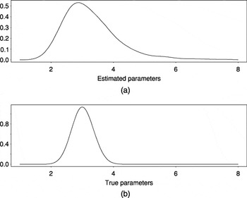
(a) Estimated sampling density of the estimator νn with n = 1,000. The true data generating process is GARCH(1,1) with α = 0.3,β = 0.3, and standard normal innovations εk. The 2.5, 25, 50, 75, and 97.5 percentiles of the sampling distribution are, respectively, 2.06, 2.68, 3.12, 3.7, and 5.62. The approximate true value of ν is 3.436. (b) Estimated sampling density of the estimator νn with n = 1,000 but with the estimators replaced by the true values β and α. The estimated densities are based on 1,000 replications of νn smoothed by a Gaussian kernel.
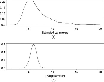
(a) Estimated sampling density of the estimator νn with n = 1,000. The true data generating process is GARCH(1,1) with α = 0.1,β = 0.8, and standard normal innovations εk. The 2.5, 25, 50, 75, and 97.5 percentiles of the sampling distribution are, respectively, 3.4, 4.82, 6.04, 7.78, and 14.04. The approximate true value of ν is 6.263. (b) Estimated sampling density of the estimator νn with n = 1,000 but with the estimators replaced by the true values β and α. The estimated densities are based on 1,000 replications of νn smoothed by a Gaussian kernel.
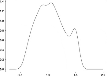
Estimated sampling density of the estimator νn with n = 1,000. The true data generating process is AR(1) with the autoregressive parameters equal to 0.5 and i.i.d. symmetric stable innovations with the index of stability equal to 1.75. The 2.5, 25, 50, 75, and 97.5 percentiles of the sampling distribution are, respectively, 0.63, 0.86, 1.05, 1.25, and 1.51. The exact true value of ν is 0.875. The estimated densities are based on 1,000 replications of νn smoothed by a Gaussian kernel.
 You have
Access
- 19
- Cited by