

1 Introduction
The flow induced in a stably stratified medium near an inclined boundary by the no-flux boundary condition is a well-known phenomenon. Contours of constant density are horizontal in the stratified ambient, but are bent to be normal to the inclined no-flux boundary, resulting in horizontal density gradients near the boundary, so that the associated baroclinic torque drives a flow in the boundary layer. Phillips (Reference Phillips1970) and Wunsch (Reference Wunsch1970) independently elaborated on this in the context of a sloping ocean bottom, and found a steady boundary layer solution for the wall-normal profile of the wall-tangent velocity as a result of a balance between viscous and buoyancy forces. Their analysis considered an infinitely long inclined wall. The induced flow is up-slope if the wall bounds the fluid from below, and down-slope if it is bounded from above. The boundary layer solution breaks down as the orientation of the no-flux wall approaches horizontal. Peacock, Stocker & Aristoff (Reference Peacock, Stocker and Aristoff2004) presented the first experimental validation of the inclination angle dependence of this solution, noting that the critical angle for solution failure is expected to depend on the strength of the stratification and the Prandtl/Schmidt number. This flow is often referred to as a diffusion-driven flow, and is often thought of as being slow. The slowness is attributed to the very large Schmidt number of salt-stratified water (of order  $10^{3}$), which is often the context that this problem is studied in.
Here, we are interested in studying this phenomenon in a controlled fully enclosed flow. There have been a number of related studies. Quon (Reference Quon1976, Reference Quon1983) presented simulations and asymptotics for a square cavity with two insulated walls and two walls with specified temperatures, corresponding to a linear temperature variation with the vertical direction, ostensibly trying to maintain a stable linear stratification. Page (Reference Page2011) studied the same problem, but over a wide range of tilt angles, overcoming the analytical difficulties Quon (Reference Quon1983) faced. These studies assumed the flow to be steady. The imposed linear temperature profiles are difficult to implement experimentally in a variable tilt angle set-up. Ulloa & Ochoa (Reference Ulloa and Ochoa1997) also considered a number of closely related configurations, having different combinations of insulating and conducting walls. They also specified the temperature on the conducting walls to correspond to a uniform stable stratification. In contrast, we are interested in specifying fixed constant temperatures on the conducting walls, and in investigating what happens as the tilt angle is varied. This is what is done with Rayleigh–Bénard convection (hot plate on the bottom, cold plate on the top) subjected to tilt, which has been studied widely and is experimentally realizable (e.g. Hart Reference Hart1971; Shishkina & Horn Reference Shishkina and Horn2016; Jiang, Sun & Calzavarini Reference Jiang, Sun and Calzavarini2019). At tilt angle  $\unicode[STIX]{x1D703}=90^{\circ }$, this set-up corresponds to the well-studied natural convection in a laterally heated cavity problem (e.g. Gill Reference Gill1966; Patterson & Imberger Reference Patterson and Imberger1980; Bejan, Al-Homoud & Imberger Reference Bejan, Al-Homoud and Imberger1981; Ivey Reference Ivey1984; Paolucci & Chenoweth Reference Paolucci and Chenoweth1989; Le Quéré & Behnia Reference Le Quéré and Behnia1998; Xin & Le Quéré Reference Xin and Le Quéré2006; Oteski et al. Reference Oteski, Duguet, Pastur and Le Quéré2015). There have also been experimental and numerical studies at selected tilt angles in the range
 $\unicode[STIX]{x1D703}\in [0^{\circ },180^{\circ }]$ (Ozoe et al. Reference Ozoe, Yamamoto, Sayama and Churchill1974; Cliffe & Winters Reference Cliffe and Winters1984; Inaba & Fukuda Reference Inaba and Fukuda1984; Baïri Reference Baïri2008; Corvaro, Paroncini & Sotte Reference Corvaro, Paroncini and Sotte2012; Torres et al. Reference Torres, Henry, Komiya, Maruyama and Ben Haldid2013), but these have either been in steady regimes or only reported time-averaged flows. Here, we investigate the situation where the cold plate is on the bottom and the hot plate is on the top, and tilt this through angles
 $0^{\circ }\leqslant \unicode[STIX]{x1D703}\leqslant 90^{\circ }$. In particular, the parameter regimes in which the resultant flow becomes unsteady are determined, the physical mechanisms responsible for the unsteadiness are described, as is how the flow transitions to the well-studied natural convection scenario as
 $\unicode[STIX]{x1D703}\rightarrow 90^{\circ }$.
2 Governing equations, symmetries and numerics
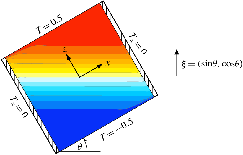
Schematic of the square cavity tilted by an angle  $\unicode[STIX]{x1D703}$ from the horizontal; the upward vertical direction is indicated by
 $\unicode[STIX]{x1D743}$. The isotherms correspond to buoyancy number
 $R_{N}=10^{4}$, Prandtl number
 $\unicode[STIX]{x1D70E}=0.71$ and tilt angle
 $\unicode[STIX]{x1D703}=30^{\circ }$, with 14 filled equispaced isotherms
 $T\in [-0.5,0.5]$, with cold as blue and hot as red.

Consider a fluid of kinematic viscosity  $\unicode[STIX]{x1D708}$, thermal diffusivity
 $\unicode[STIX]{x1D705}$ and coefficient of volume expansion
 $\unicode[STIX]{x1D6FD}$ contained in a square cavity of side lengths
 $L$ that is inclined to the horizontal by an angle
 $\unicode[STIX]{x1D703}$; see figure 1. Two opposite walls of the cavity are insulated and the other two are held at different fixed temperatures. When the inclination angle
 $\unicode[STIX]{x1D703}=0^{\circ }$, the insulated walls are the vertical walls, and the top and bottom walls are at fixed temperatures
 $T_{hot}$ and
 $T_{cold}$ respectively, such that
 $\unicode[STIX]{x0394}T=T_{hot}-T_{cold}>0$. Gravity
 $g$ acts in the downward vertical direction. In the absence of any other external force, the fluid is linearly stratified.
The non-dimensional temperature is  $T=(T^{\ast }-T_{cold})/\unicode[STIX]{x0394}T-0.5$, where
 $T^{\ast }$ is the dimensional temperature. Length is scaled by
 $L$ and time by
 $1/N$, where
 $N=\sqrt{g\unicode[STIX]{x1D6FD}\unicode[STIX]{x0394}T/L}$ is the buoyancy frequency. A two-dimensional Cartesian coordinate system
 $\text{x}=(x,z)\in [-0.5,0.5]\times [-0.5,0.5]$ is attached to the cavity with its origin at the centre and the directions
 $x$ and
 $z$ aligned with the sides. In this non-dimensional reference frame, the velocity is
 $\text{u}=(u,w)$, and the unit vector in the upward vertical direction is
 $\unicode[STIX]{x1D743}=(\sin \unicode[STIX]{x1D703},\cos \unicode[STIX]{x1D703})$. The velocity boundary condition is no slip on all walls. The insulated walls have zero heat flux:
 $T_{x}=0$ at
 $x=\pm 0.5$, and the conducting walls have fixed temperatures:
 $T=\pm 0.5$ at
 $z=\pm 0.5$.
Under the Boussinesq approximation, the non-dimensional governing equations are
 $$\begin{eqnarray}\left.\begin{array}{@{}c@{}}\displaystyle \text{u}_{t}+\text{u}\boldsymbol{\cdot }\unicode[STIX]{x1D735}\text{u}=-\unicode[STIX]{x1D735}p+\frac{1}{R_{N}}\unicode[STIX]{x1D6FB}^{2}\text{u}+T\unicode[STIX]{x1D743},\quad \unicode[STIX]{x1D735}\boldsymbol{\cdot }\text{u}=0,\\ \displaystyle T_{t}+\text{u}\boldsymbol{\cdot }\unicode[STIX]{x1D735}T=\frac{1}{\unicode[STIX]{x1D70E}R_{N}}\unicode[STIX]{x1D6FB}^{2}T,\end{array}\right\}\end{eqnarray}$$
where  $p$ is the reduced pressure, the buoyancy number
 $R_{N}=NL^{2}/\unicode[STIX]{x1D708}$ is the ratio of the viscous and buoyancy time scales (it is the square root of the Grashof number) and
 $\unicode[STIX]{x1D70E}=\unicode[STIX]{x1D708}/\unicode[STIX]{x1D705}$ is the Prandtl number. Here, we fix
 $\unicode[STIX]{x1D70E}=0.71$ (air at room temperature), and consider
 $R_{N}\in [1,10^{6}]$ and
 $\unicode[STIX]{x1D703}\in [0^{\circ },90^{\circ }]$. When
 $\unicode[STIX]{x1D703}=0^{\circ }$, the static linear stratified equilibrium
 $(\text{u}=\mathbf{0},\,T=z)$ is a solution of (2.1). For
 $\unicode[STIX]{x1D703}>0^{\circ }$ with
 $R_{N}>0$, the static equilibrium no longer exists and the resulting solutions are non-trivial.
The system (2.1) together with the boundary conditions described above is invariant to a centrosymmetry, corresponding to reflection through the origin. The action of this symmetry is
 $$\begin{eqnarray}{\mathcal{C}}:[u,w,T](x,z,t)\mapsto [-u,-w,-T](-x,-z,t).\end{eqnarray}$$
All observed steady states  $S$ have this invariance. Time periodic states that bifurcate from a steady state via Hopf bifurcations come in two flavours. Either the limit cycle preserves this symmetry instantaneously, in which case we say that it is pointwise invariant, or it does not. Limit cycles that are not pointwise invariant may instead be setwise invariant, whereby they are invariant to a spatio-temporal symmetry consisting of
 ${\mathcal{C}}$ composed with a half-period translation in time. The action of this spatio-temporal symmetry is
 $$\begin{eqnarray}{\mathcal{C}}_{st}:[u,w,T](x,z,t)\mapsto [-u,-w,-T](-x,-z,t+\unicode[STIX]{x1D70F}/2),\end{eqnarray}$$
where  $\unicode[STIX]{x1D70F}$ is the period of the limit cycle.
The heat fluxes needed to maintain the constant temperatures at the hot and cold walls at  $z=\pm 0.5$ are quantified by the Nusselt numbers
 $$\begin{eqnarray}Nu_{h}=\int _{-0.5}^{0.5}T_{z}(x,0.5)\,\text{d}x\quad \text{and}\quad Nu_{c}=\int _{-0.5}^{0.5}T_{z}(x,-0.5)\,\text{d}x,\end{eqnarray}$$
where  $T_{z}(x,\pm 0.5)$ is the normal gradient of the temperature evaluated at the corresponding conducting walls
 $z=\pm 0.5$. For the static state at
 $\unicode[STIX]{x1D703}=0^{\circ }$,
 $T(x,z)=z$ and so
 $Nu_{h}=Nu_{c}=1$. When
 $\unicode[STIX]{x1D703}>0^{\circ }$, the steady states have
 $Nu_{h}=Nu_{c}>1$. For unsteady flows,
 $Nu_{h}$ and
 $Nu_{c}$ are unsteady and in general differ at any instant in time, but their long-time averages are the same. For limit cycles,
 $Nu_{h}$ and
 $Nu_{c}$ are periodic, and if the limit cycle is pointwise invariant they are in phase whereas for setwise invariant limit cycles,
 $Nu_{h}$ and
 $Nu_{c}$ are half a period out of phase. This phase information on the heat fluxes provides a convenient way to determine the spatio-temporal symmetry of a limit cycle.
The governing equations are solved numerically using a spectral-collocation method. It is the same technique as was used in Wu, Welfert & Lopez (Reference Wu, Welfert and Lopez2018) and Yalim, Welfert & Lopez (Reference Yalim, Welfert and Lopez2019). Briefly, the velocity, pressure and temperature are approximated by polynomials of degree  $n$, associated with the Chebyshev–Gauss–Lobatto grid. A fractional-step improved projection method, based on a linearly implicit and stiffly stable second-order accurate scheme, is used to integrate in time with time step
 $\unicode[STIX]{x1D6FF}t$. For
 $R_{N}\leqslant 3\times 10^{4}$, the spatial and temporal resolution used was
 $n=72$ and
 $\unicode[STIX]{x1D6FF}t=2\times 10^{-7}R_{N}$. For
 $R_{N}>3\times 10^{4}$, the resolution was increased up to
 $n=512$ and
 $\unicode[STIX]{x1D6FF}t=5\times 10^{-9}R_{N}$.
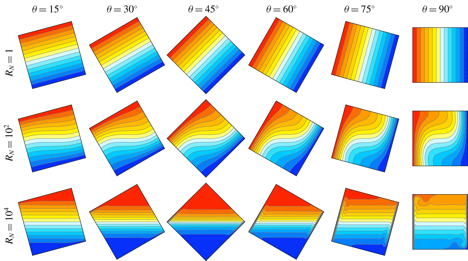
Isotherms of the steady states S at the indicated  $\unicode[STIX]{x1D703}$ and
 $R_{N}$, showing 14 filled equispaced isotherms in
 $T\in [-0.5,0.5]$, with cold as blue and hot as red. The online movie ‘Movie 1’ (available at https://doi.org/10.1017/jfm.2019.913) animates the isotherms and vorticity of the steady states at
 $R_{N}=2\times 10^{4}$ over
 $\unicode[STIX]{x1D703}\in [0^{\circ },90^{\circ }]$; unstable steady states were computed using selective frequency damping.

3 Static and steady states
For the untilted problem with  $\unicode[STIX]{x1D703}=0^{\circ }$, the static linear stratified equilibrium (
 $\text{u}=\mathbf{0}$,
 $T=z$) is stable for all
 $R_{N}$ and
 $\unicode[STIX]{x1D70E}$. It is also the stable equilibrium for all
 $\unicode[STIX]{x1D703}$ and
 $\unicode[STIX]{x1D70E}$ in the limit
 $R_{N}\rightarrow 0$. For any
 $R_{N}>0$ and
 $\unicode[STIX]{x1D703}>0^{\circ }$, this static equilibrium is no longer a solution. For very small
 $R_{N}$, the isotherms are essentially linear in
 $z$, irrespective of the tilt, as can be seen in figure 2 for
 $R_{N}=1$. For such small
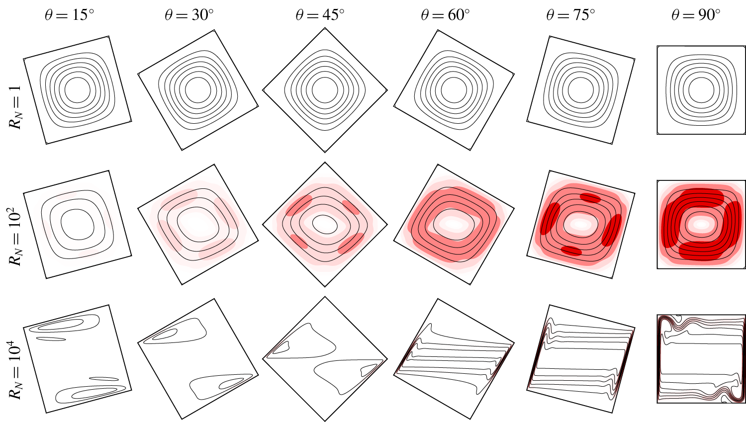
 $R_{N}$, the flow is very slow and consists of a weak clockwise circulation centred at the origin; as illustrated by the corresponding streamlines in figure 3. The streamlines are isocontours of the streamfunction
 $\unicode[STIX]{x1D713}$, which is obtained by solving
 $$\begin{eqnarray}\unicode[STIX]{x1D6FB}^{2}\unicode[STIX]{x1D713}=-\unicode[STIX]{x1D702},\quad \unicode[STIX]{x1D713}(x,\pm 0.5)=\unicode[STIX]{x1D713}(\pm 0.5,z)=0,\end{eqnarray}$$
where  $\unicode[STIX]{x1D702}=u_{z}-v_{x}$ is the vorticity. This Poisson equation is solved using diagonalization of the second-order pseudospectral operators, as in the main solver. Except for large
 $R_{N}$ and
 $\unicode[STIX]{x1D703}\approx 90^{\circ }$, the streamfunction
 $\unicode[STIX]{x1D713}$ is positive everywhere in the cavity and the flow is in the clockwise direction. The streamfunction isocontours are equispaced linearly, such that the local speed is inversely proportional to the spacing between the streamlines, and the velocity vector is locally tangent to the streamlines. The speed is given by
 $\sqrt{2E}$, the kinetic energy
 $E$ is also included in figure 3.
Kinetic energy  $E$ and scaled streamfunction
 $\unicode[STIX]{x1D713}/\sin \unicode[STIX]{x1D703}$, corresponding to the steady flows shown in figure 2.
 $E$ is represented with seven red filled log-spaced contours in the range
 $E\in [3.5\times 10^{-5},3.5\times 10^{-2}]$, where
 $E_{max}=3.5\times 10^{-2}$. There are eight equispaced streamlines with
 $\unicode[STIX]{x1D713}\in [0,\unicode[STIX]{x1D713}_{max}]$ where
 $\unicode[STIX]{x1D713}_{max}=1.3\times 10^{-3}$,
 $6.2\times 10^{-2}$ and
 $7\times 10^{-3}$ for
 $R_{N}=1$,
 $10^{2}$ and
 $10^{4}$ respectively.

Increasing  $R_{N}$ to
 $10^{2}$ results in a relatively faster flow. The nonlinear terms in the governing equations are no longer negligible and the isotherms begin bending about the centre of the cavity due to advection. The bending increases with the tilt angle
 $\unicode[STIX]{x1D703}$ and the isotherms tend to be horizontal near the origin. The isotherms cannot be horizontal all the way out to the cavity walls due to the thermal boundary conditions. On the hot and cold walls the isotherms must be tangential and also must approach the insulated walls orthogonally. These constraints result in temperature gradients near the walls which baroclinically drive the circulation. The boundary flows on the insulated and fixed temperature walls are quite similar, as can be seen from the streamlines at
 $R_{N}=10^{2}$. However, the details of the boundary layers are quite different. On the insulated walls, the bending of the isotherms into the horizontal in the interior together with the boundary constrain them to meet the insulated walls orthogonally. This causes the isotherms to bunch up towards the two corners
 $(x,z)=(\pm 0.5,\pm 0.5)$ on the insulated walls at
 $x=\mp 0.5$, resulting in larger horizontal temperature gradients (and hence faster flows) than near the other two corners at
 $(x,z)=(\pm 0.5,\mp 0.5)$. On the conducting walls, this means that the heat flux required to maintain the fixed temperature is greatest near the two opposite corners
 $(x,z)=(\pm 0.5,\pm 0.5)$.
For  $R_{N}>10^{2}$, buoyancy effects dominate over diffusive effects. The stronger stratification results in the horizontal isotherms extending further out from the centre and the interior becomes more vertically stratified, albeit in a nonlinear way. This is clearly seen in the isotherms at
 $R_{N}=10^{4}$ shown in figure 2. Also, the flow is no longer a simple circulation about the centre of the cavity. Instead, at higher
 $R_{N}$ the flow is predominately in the boundary layers on the conducting walls, with very different characteristics between the flows for
 $\unicode[STIX]{x1D703}<45^{\circ }$ and
 $\unicode[STIX]{x1D703}>45^{\circ }$. As
 $\unicode[STIX]{x1D703}$ and
 $R_{N}$ are increased, the contribution from bent isotherms to the horizontal temperature gradient becomes negligible compared to the horizontal component of the temperature stratification. One striking feature of these higher
 $R_{N}$ flows is the presence of triangular isothermal regions near the two corners
 $(x,z)=(\pm 0.5,\mp 0.5)$; these regions being largest for
 $\unicode[STIX]{x1D703}=45^{\circ }$. Their presence is due to the large gradients in temperature near the two corners
 $(x,z)=(\pm 0.5,\pm 0.5)$ on the insulated walls, noted earlier for lower
 $R_{N}$. The near constant temperature in these regions is consistent with the wall temperature being constant, and since the temperature is very close to being constant near the insulated walls in these regions, the no-flux condition is also satisfied. These triangular isothermal regions vanish as
 $\unicode[STIX]{x1D703}$ approaches
 $0^{\circ }$ or
 $90^{\circ }$, and their vertical extent is maximal at
 $\unicode[STIX]{x1D703}=45^{\circ }$.
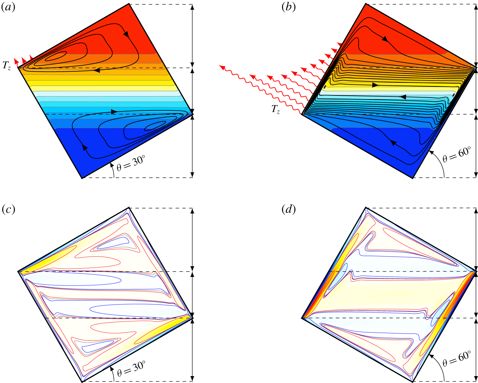
Steady states S at  $R_{N}=10^{4}$,
 $\unicode[STIX]{x1D70E}=0.71$, and
 $\unicode[STIX]{x1D703}$ as indicated. (a,b) Isotherms with superimposed streamlines (fourteen equispaced isotherms
 $T\in [-0.5,0.5]$ and streamlines
 $\unicode[STIX]{x1D713}\in [0,3.7\times 10^{-3}]$), and (c,d) the corresponding vorticity with symmetric log-spaced filled contours normalized by the absolute maximum vorticity of (d), and the contour lines are at
 $\pm 10^{-n}\unicode[STIX]{x1D702}_{max}$ with
 $n=1$, 2, 3 and 4 and
 $\unicode[STIX]{x1D702}_{max}=36.5$. The red (blue) lines are positive (negative)
 $\unicode[STIX]{x1D702}$, and the
 $\unicode[STIX]{x1D702}=0$ contour is grey. Also shown schematically, but drawn to scale, is the heat flux
 $T_{z}$ along the hot wall; the length of each wiggly arrow is proportional to the local heat flux.

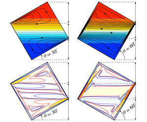
Figure 4 illustrates the fundamental differences between the  $\unicode[STIX]{x1D703}<45^{\circ }$ and
 $\unicode[STIX]{x1D703}>45^{\circ }$ flows for high
 $R_{N}$, using typical steady states at
 $\unicode[STIX]{x1D703}=30^{\circ }$ and
 $60^{\circ }$, both at
 $R_{N}=10^{4}$. The isotherms together with superimposed streamlines are shown in figure 4(a,b). Also shown schematically, but drawn to scale, is the heat flux
 $T_{z}$ along the hot wall. The isolevels for the streamlines are the same in both plots, showing that the
 $\unicode[STIX]{x1D703}=60^{\circ }$ flow is much faster that the
 $\unicode[STIX]{x1D703}=30^{\circ }$ flow. In both cases the temperature distribution is similarly partitioned into two near isothermal triangular regions near the two corners at
 $(x,z)=(\pm 0.5,\pm 0.5)$, separated by a central, almost linearly stratified region. The vertical extent (
 $\unicode[STIX]{x1D709}=\sqrt{x^{2}+z^{2}}$) of the isothermal regions is
 $0\lesssim \unicode[STIX]{x1D709}\lesssim \sin \unicode[STIX]{x1D703}$ for
 $\unicode[STIX]{x1D703}<45^{\circ }$ and
 $0\lesssim \unicode[STIX]{x1D709}\lesssim \cos \unicode[STIX]{x1D703}$ for
 $\unicode[STIX]{x1D703}>45^{\circ }$, and the central stratified regions have vertical extent
 $|\text{sin}\,\unicode[STIX]{x1D703}-\cos \unicode[STIX]{x1D703}|=\sqrt{2}|\text{sin}\,(\unicode[STIX]{x1D703}-45^{\circ })|$.
The flow in the central region differs significantly depending on  $\unicode[STIX]{x1D703}$. For
 $\unicode[STIX]{x1D703}=30^{\circ }$ (in general, for
 $\unicode[STIX]{x1D703}<45^{\circ }$), the horizontal temperature gradients on the hot and cold walls at
 $z=\pm 0.5$ near the two corners
 $(x,z)=(\mp 0.5,\pm 0.5)$ lead to the baroclinic production of vorticity. This locally produced vorticity (shown in figure 4c) drives fast boundary layer flows on the hot and cold walls, which are turned when they reach the two corners
 $(x,z)=(\pm 0.5,\pm 0.5)$, and then return horizontally back to the corners from which they originated, leaving the central stratified region essentially stagnant. The vorticity plot reveals a pair of weak horizontal shear layers separating the central stagnant region and the upper and lower isothermal regions. These shear layers are strongest near the two corners
 $(x,z)=(\pm 0.5,\mp 0.5)$. They connect these corners horizontally to the insulated walls at
 $x=\pm 0.5$. The corner at
 $(x,z)=(-0.5,0.5)$ is higher than the corner at
 $(x,z)=(0.5,-0.5)$, so that the central stratified region is bounded horizontally by portions of the insulated walls. In contrast, for
 $\unicode[STIX]{x1D703}=60^{\circ }$ (in general, for
 $\unicode[STIX]{x1D703}>45^{\circ }$), the central stratified region is bounded horizontally by portions of the hot and cold walls at
 $z=\pm 0.5$. This sets up a natural convection scenario (albeit with slanted walls) that drives strong boundary layer flows up the hot wall and down the cold wall, with the flow into and out of these boundary layers being replenished by slower horizontal flow between the two walls, with the isotherms in this interior central region also being horizontal (Gill Reference Gill1966). Although this interior horizontal flow is much slower that the flow in the boundary layers, it is significantly faster that the flow in the triangular isothermal regions, which has speed comparable to those in the isothermal regions for
 $\unicode[STIX]{x1D703}<45^{\circ }$. The boundary layer flows at the hot and cold walls have strong associated temperature gradients, resulting in a heat flux at the hot and cold walls which is an order of magnitude larger than that for
 $\unicode[STIX]{x1D703}=30^{\circ }$.
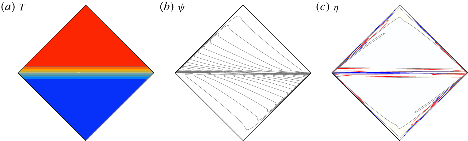
Isotherms, streamlines and vorticity of the steady state S at  $R_{N}=10^{6}$ and
 $\unicode[STIX]{x1D703}=45^{\circ }$. There are 14 equispaced isotherms
 $T\in [-0.5,0.5]$ and streamlines
 $\unicode[STIX]{x1D713}\in [0,7\times 10^{-5}]$. The vorticity contours are symmetric log spaced and based on the absolute maximum vorticity,
 $\unicode[STIX]{x1D702}_{max}=117.7$; the contour lines are at
 $\pm 10^{n}\unicode[STIX]{x1D702}_{max}$ with
 $n=1$, 2, 3 and 4. The red (blue) contour lines are positive (negative), and the
 $\unicode[STIX]{x1D702}=0$ contour is grey.

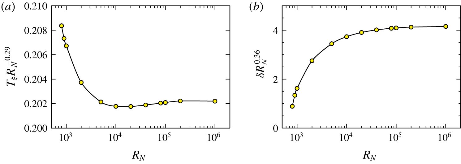
Variations with  $R_{N}$ of (a) the vertical temperature gradient at the centre of the container,
 $T_{\unicode[STIX]{x1D709}}$, and (b) the half-thickness of the shear layer,
 $\unicode[STIX]{x1D6FF}$, for
 $\unicode[STIX]{x1D703}=45^{\circ }$. The results are plotted to reveal the power laws
 $T_{\unicode[STIX]{x1D709}}\approx 0.2R_{N}^{\;0.29}$ and
 $\unicode[STIX]{x1D6FF}\approx 4R_{N}^{-0.36}$ as
 $R_{N}$ becomes large.

The case  $\unicode[STIX]{x1D703}=45^{\circ }$ is particular in that the vertical extent of the central stratified region becomes vanishingly small with increasing
 $R_{N}$, with the two corners
 $(x,z)=(\pm 0.5,\mp 0.5)$ being at the same height. The upper and lower triangular regions are essentially isothermal at the temperature of the corresponding hot and cold walls. The isotherms of the steady state at
 $R_{N}=10^{6}$ are shown in figure 5(a). The fluid is almost stagnant in these regions, which are separated by a strong horizontal shear layer, with the flow from left-to-right above it and right-to-left below it. The fluid in this shear layer flows into the two corners
 $(x,z)=(\pm 0.5,\mp 0.5)$, and is then turned into thin boundary layers along the hot and cold walls. There is a slow flow from these boundary layers back into the shear layer. The corresponding streamlines in figure 5(b) illustrate this flow. The half-thickness
 $\unicode[STIX]{x1D6FF}$ of this shear layer is quantified by the vertical distance from the origin to the first zero in the vorticity (shown in figure 5c). Figure 6 shows how the vertical temperature gradient at the origin, denoted
 $T_{\unicode[STIX]{x1D709}}$, and
 $\unicode[STIX]{x1D6FF}$ vary with
 $R_{N}$ for
 $\unicode[STIX]{x1D703}=45^{\circ }$. It is apparent that an asymptotic regime is reached for
 $R_{N}>10^{5}$, with power laws
 $T_{\unicode[STIX]{x1D709}}\approx 0.2R_{N}^{0.29}$ and
 $\unicode[STIX]{x1D6FF}\approx 4R_{N}^{-0.36}$. These indicate that the shear layer thickness
 $\unicode[STIX]{x1D6FF}$ vanishes faster than the temperature gradient
 $T_{\unicode[STIX]{x1D709}}$ becomes unbounded as
 $R_{N}$ increases.
4 Unsteady periodic flows
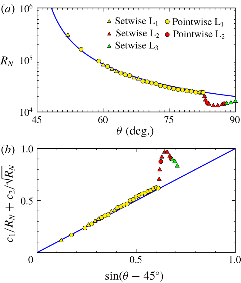
(a) Loci of the first limit cycle (filled markers) for given  $\unicode[STIX]{x1D703}$ as
 $R_{N}$ is increased, and (b) the fit
 $7000/R_{N}+50/\sqrt{R_{N}}=\sin (\unicode[STIX]{x1D703}-45^{\circ })$ (blue curve), also shown in (a).

For tilt angles  $\unicode[STIX]{x1D703}<45^{\circ }$, the flow remains steady for all
 $R_{N}$ considered (
 $R_{N}\leqslant 10^{6}$). However, for
 $\unicode[STIX]{x1D703}>45^{\circ }$ the steady state S loses stability as
 $R_{N}$ is increased above a critical value that depends on
 $\unicode[STIX]{x1D703}$. Figure 7(a) shows the loci of the first limit cycles (yellow symbols) for a given
 $\unicode[STIX]{x1D703}$ as
 $R_{N}$ is increased. The blue line in the figure is the fit
 $7000/R_{N}+50/\sqrt{R_{N}}=\sin (\unicode[STIX]{x1D703}-45^{\circ })$ which collapses the loci (for
 $\unicode[STIX]{x1D703}\lesssim 82.5^{\circ }$) onto a straight line, as shown in figure 7(b). The
 $O(1/\sqrt{R_{N}})$ contribution in the fit reflects the dominance of nonlinear effects at large
 $R_{N}$, while the
 $O(1/R_{N})$ term corresponds to linear viscous contributions. The former dominates as soon as
 $R_{N}\gtrsim 15\,600$, but still accounts for only
 $67\,\%$ at the onset of instability for
 $\unicode[STIX]{x1D703}=60^{\circ }$ and
 $R_{N}\approx 8\times 10^{4}$ (i.e.
 $(50/\sqrt{R_{N}})/(7000/R_{N}+50/\sqrt{R_{N}})\approx 0.67$ for
 $R_{N}\approx 8\times 10^{4}$). This suggests that both viscous and nonlinear terms contribute non-trivially at onset. The fit also emphasizes the fact that the flow remains steady at tilt angle
 $\unicode[STIX]{x1D703}=45^{\circ }$ and that a small but increasing amount of viscosity (decreasing
 $R_{N}$) is needed to stabilize the flow as
 $\unicode[STIX]{x1D703}$ increases from
 $45^{\circ }$.
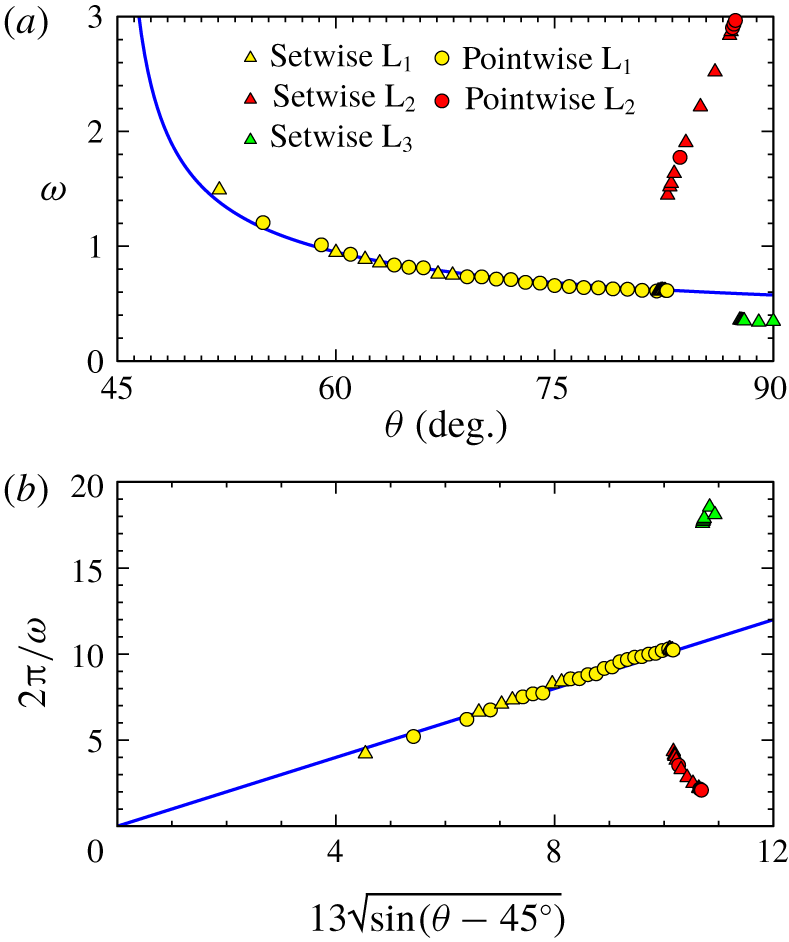
(a) Variation of the frequency  $\unicode[STIX]{x1D714}$ of limit cycles
 $\text{L}_{1}$,
 $\text{L}_{2}$ and
 $\text{L}_{3}$ (symbols) with
 $\unicode[STIX]{x1D703}$ at onset (
 $R_{N}$ just above the critical values shown in figure 7), together with the fit
 $2\unicode[STIX]{x03C0}/\unicode[STIX]{x1D714}=13\sqrt{\sin (\unicode[STIX]{x1D703}-45^{\circ })}$; (b) same data as in (a).

The steady state loses stability via supercritical Hopf bifurcations for tilt angles  $45^{\circ }<\unicode[STIX]{x1D703}\leqslant 90^{\circ }$ as
 $R_{N}$ is increased above a critical
 $\unicode[STIX]{x1D703}$-dependent value, spawning a stable limit cycle. Figure 8(a) shows the limit cycle frequency as a function of tilt angle
 $\unicode[STIX]{x1D703}$. There are three distinct ranges:
 $\unicode[STIX]{x1D703}\in (45^{\circ },82^{\circ }]$,
 $\unicode[STIX]{x1D703}\in [83^{\circ },87^{\circ }]$ and
 $\unicode[STIX]{x1D703}\in [88^{\circ },90^{\circ }]$. These correspond to three distinct limit cycles, referred to as
 $\text{L}_{1}$,
 $\text{L}_{2}$ and
 $\text{L}_{3}$. Figure 8(b) provides a fit
 $2\unicode[STIX]{x03C0}/\unicode[STIX]{x1D714}=13\sqrt{\sin (\unicode[STIX]{x1D703}-45^{\circ })}$ for the period of
 $\text{L}_{1}$ along the critical curve.
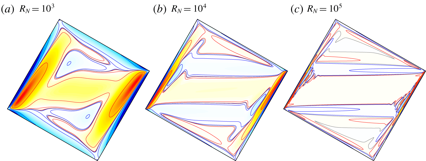
Vorticity of steady states S at  $\unicode[STIX]{x1D703}=60^{\circ }$ for
 $R_{N}$ as indicated. The filled contours are symmetric log spaced based on the absolute maximum vorticity,
 $\unicode[STIX]{x1D702}_{max}=10.7$,
 $36.5$ and
 $120.1$ for (a), (b) and (c) respectively. The contour levels are at
 $\pm 10^{-n}\unicode[STIX]{x1D702}_{max}$ with
 $n=1$, 2, 3 and 4. The red (blue) lines are positive (negative), and the
 $\unicode[STIX]{x1D702}=0$ contour is grey. Note that the conducting hot wall is along the ‘upper left’.

Figure 9 illustrates how the  $\text{L}_{1}$ instability develops with increasing
 $R_{N}$ for
 $\unicode[STIX]{x1D703}=60^{\circ }$. At relatively low
 $R_{N}=10^{3}$, the imbalance between the boundary layer flows on the constant temperature walls and the insulated walls is evident. From the two corners at
 $(\pm 0.5,\mp 0.5)$, the zero vorticity contour meanders out horizontally towards the opposite constant temperature wall, but dwindles before reaching the wall. Increasing
 $R_{N}$ to
 $10^{4}$, the
 $\unicode[STIX]{x1D702}=0$ contour comes straight out of the corners and proceeds horizontally until it reaches the boundary layer on the opposite constant temperature wall, which is much thinner and more intense at this larger
 $R_{N}$. The associated streamlines (shown in figure 3) indicate that the flows near these horizontal
 $\unicode[STIX]{x1D702}=0$ contours are horizontal shear flows, and that outside of these internal shear layers and the boundary layers, the flow is essentially stagnant, as is to be expected for a steady strongly stratified flow. Where these horizontal shear layers meet the constant temperature wall boundary layers, the boundary layers are locally perturbed. The steady state S loses stability to the
 $\text{L}_{1}$ limit cycle at
 $R_{N}\approx 8\times 10^{4}$. By using selective frequency damping (Åkervik et al. Reference Åkervik, Brandt, Henningson, Hœpffner, Marxen and Schlatter2006; Lopez et al. Reference Lopez, Welfert, Wu and Yalim2017), we have also computed the unstable steady states beyond the critical
 $R_{N}$. Figure 9 shows the vorticity of the unstable steady state at
 $R_{N}=10^{5}$. The horizontal shear layers are much sharper and the localized undulations in the constant temperature wall boundary layers are more clearly evident.
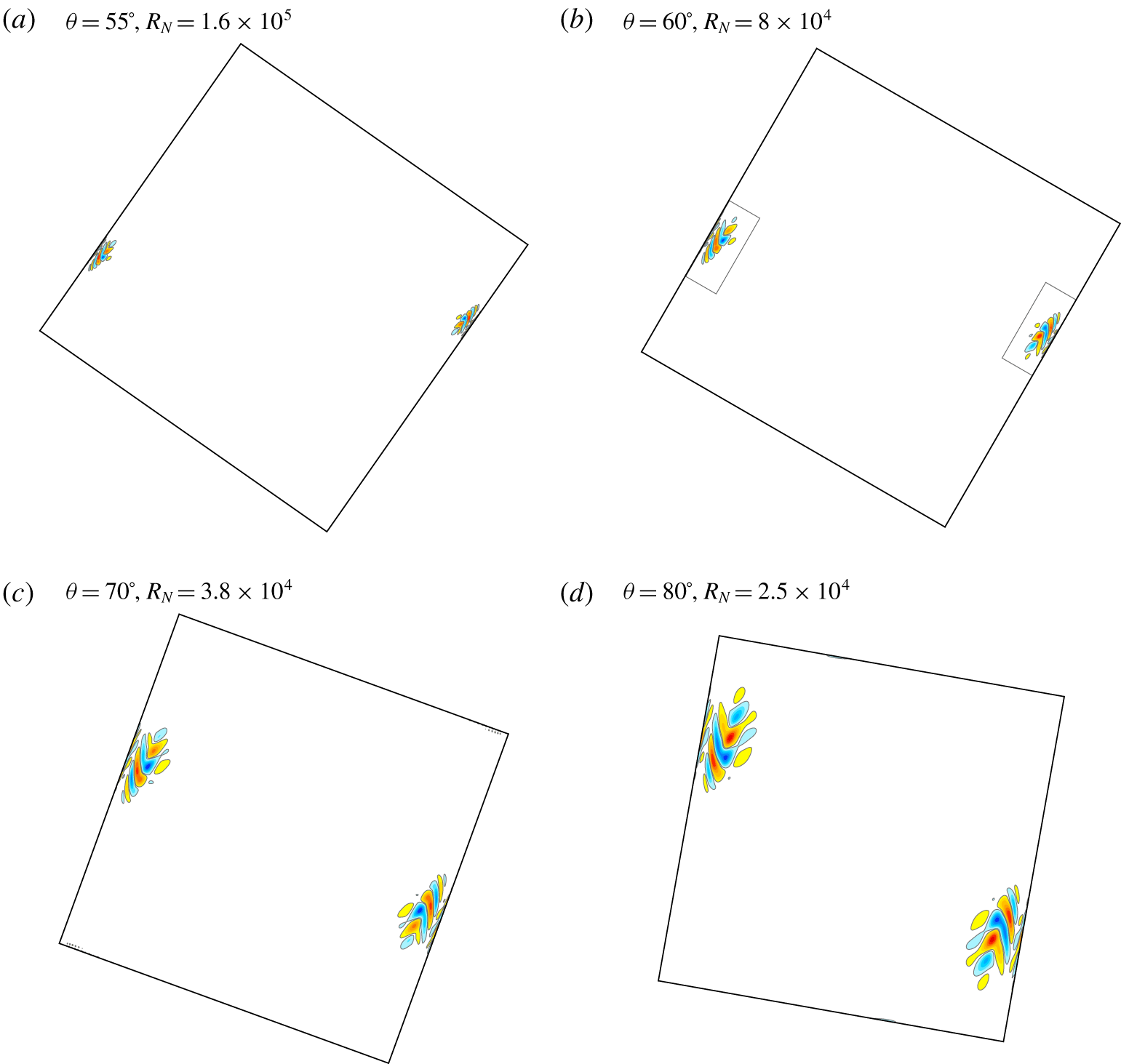
Snapshots of the perturbation vorticity of  $\text{L}_{1}$ for
 $\unicode[STIX]{x1D703}$ and
 $R_{N}$ just above onset, as indicated. The rectangular regions in (b) outlined in grey are further examined in figure 13.

To examine the spatio-temporal nature of the instability, we use the perturbation vorticity,  $\unicode[STIX]{x1D702}-\unicode[STIX]{x1D702}_{s}$, where
 $\unicode[STIX]{x1D702}_{s}$ is the vorticity of the unstable steady state S. The perturbation vorticity for
 $\text{L}_{1}$ consists of two localized standing wave packets, one on each of the hot and cold fixed temperature walls. Their locations on the respective walls correspond to the vertical level of the two corners at
 $(x,z)=(\pm 0.5,\mp 0.5)$, with downward (upward) phase velocity on the hot (cold) wall at
 $z=+0.5$ (
 $z=-0.5$). Figure 10 shows snapshots of the perturbation vorticity of
 $\text{L}_{1}$ near onset for a few tilt angles, illustrating that the size of the associated disturbance wave packets grows with the tilt angle, and its location moves up (down) the hot (cold) wall with increasing
 $\unicode[STIX]{x1D703}$.
Closer inspection of  $\text{L}_{1}$ near onset for various tilt angles reveals that it comes in two flavours: one is pointwise
 ${\mathcal{C}}$-invariant and the other is setwise
 ${\mathcal{C}}_{st}$-invariant. Which one bifurcates first from the steady state S depends on the parameters
 $\unicode[STIX]{x1D703}$ and
 $R_{N}$. In figures 7 and 8, different symbols are used to designate pointwise (circles) or setwise (triangles) limit cycles; there does not seem to be a regular pattern for which type bifurcates first from the steady state S. For
 $\unicode[STIX]{x1D703}=60^{\circ }$, the setwise
 $\text{L}_{1}$ is the first to bifurcate as
 $R_{N}$ is increased. Of the four cases shown in figure 10,
 $\text{L}_{1}$ at
 $\unicode[STIX]{x1D703}=55^{\circ }$,
 $70^{\circ }$ and
 $80^{\circ }$ is pointwise invariant, whereas for
 $\unicode[STIX]{x1D703}=60^{\circ }$ it is setwise invariant.
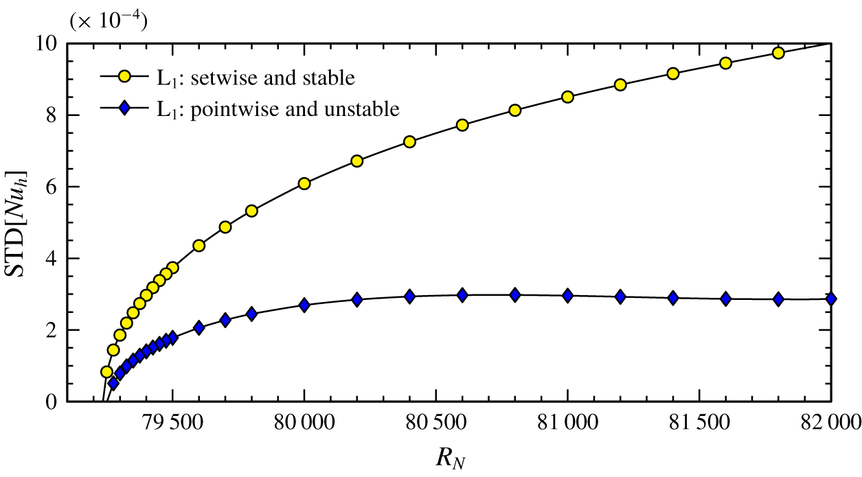
Standard deviation of the hot wall Nusselt number,  ${\rm \small{STD}}[Nu_{h}]$, for
 $\text{L}_{1}$ near onset at
 $\unicode[STIX]{x1D703}=60^{\circ }$. The setwise invariant
 $\text{L}_{1}$ is the first to bifurcate at
 $R_{N}\approx 79\,235$, followed by the pointwise invariant
 $\text{L}_{1}$ at
 $R_{N}\approx 79\,251$. The pointwise invariant
 $\text{L}_{1}$ is unstable, but it is stable in the
 ${\mathcal{C}}$-invariant subspace.

For the  $\unicode[STIX]{x1D703}=60^{\circ }$ case, we have also restricted the simulations to the
 ${\mathcal{C}}$-invariant subspace, in which the setwise
 $\text{L}_{1}$ does not exist, and found that the pointwise
 $\text{L}_{1}$ bifurcates at an
 $R_{N}$ slightly larger than the critical
 $R_{N}$ for the setwise
 $\text{L}_{1}$ in the full space. Figure 11 shows the standard deviation of the hot wall Nusselt number,
 ${\rm \small{STD}}[Nu_{h}]$, for the setwise and pointwise
 $\text{L}_{1}$ limit cycles near onset for
 $\unicode[STIX]{x1D703}=60^{\circ }$. The time averages (means) of
 $Nu_{h}$ are the same for both
 $\text{L}_{1}$ limit cycles, and grow linearly with
 $R_{N}$, from
 $Nu_{h}=42.25$ at
 $R_{N}=79\,300$ to
 $Nu_{h}=43.00$ at
 $R_{N}=82\,000$. The standard deviation
 ${\rm \small{STD}}[Nu_{h}]$, a measure of the oscillation amplitude, is less than
 $0.001\,\%$ of the mean for both limit cycles over this range of
 $R_{N}$. The oscillations have very small amplitude and are localized in space. The setwise
 $\text{L}_{1}$ at
 $\unicode[STIX]{x1D703}=60^{\circ }$ bifurcates at a supercritical Hopf bifurcation at
 $R_{N}\approx 79\,235$, and the pointwise
 $\text{L}_{1}$ also bifurcates at a supercritical Hopf bifurcation from the now unstable steady state S at
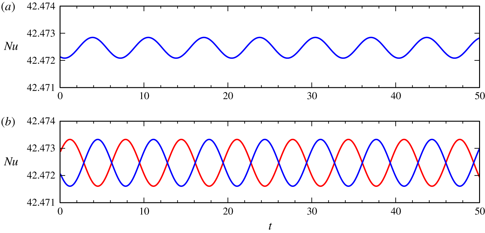
 $R_{N}\approx 79\,251$. Figure 12 shows the temporal variations of the Nusselt numbers on the hot and cold walls for the pointwise
 $\text{L}_{1}$ and setwise
 $\text{L}_{1}$ at
 $\unicode[STIX]{x1D703}=60^{\circ }$ and
 $R_{N}=8\times 10^{4}$. The pointwise
 $\text{L}_{1}$ has
 $Nu_{h}(t)=Nu_{c}(t)$ and the two time series are exactly the same. The setwise
 $\text{L}_{1}$ has
 $Nu_{h}(t)=Nu_{c}(t+\unicode[STIX]{x1D70F}/2)$. The oscillation period
 $\unicode[STIX]{x1D70F}$ is almost identical for the pointwise
 $\text{L}_{1}$ and setwise
 $\text{L}_{1}$. This means that the onset of instability for
 $\text{L}_{1}$ is close to a 1 : 1 resonant double-Hopf bifurcation between the pointwise
 $\text{L}_{1}$ and setwise
 $\text{L}_{1}$.
Time series of Nusselt numbers on the hot (red) and cold (blue) walls for (a) pointwise invariant  $\text{L}_{1}$ and (b) setwise invariant
 $\text{L}_{1}$, at
 $\unicode[STIX]{x1D703}=60^{\circ }$ and
 $R_{N}=8\times 10^{4}$.

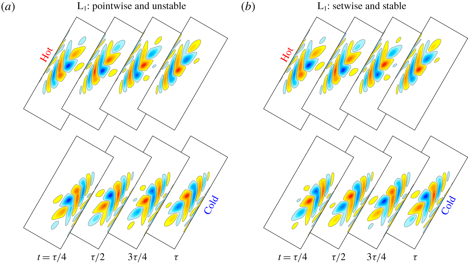
Zoomed snapshots of the perturbation vorticity  $\unicode[STIX]{x1D703}=60^{\circ }$ and
 $R_{N}=8\times 10^{4}$ over one period for (a) pointwise invariant
 $\text{L}_{1}$, and (b) setwise invariant
 $\text{L}_{1}$. The first row focuses on a region at the hot wall (
 $x\in [-0.35,0.05]$ and
 $z\in [0.4,0.5]$) and the second row focuses on the centrosymmetry-related region at the cold wall (
 $x\in [-0.05,0.35]$ and
 $z\in [-0.5,-0.4]$). These are the regions indicated in figure 10(b). See the online movie ‘Movie 2’ for an animation of the two flows in the entire container.

Spatio-temporal details of the pointwise  $\text{L}_{1}$ and setwise
 $\text{L}_{1}$ at
 $\unicode[STIX]{x1D703}=60^{\circ }$ and
 $R_{N}=8\times 10^{4}$ are shown in figure 13. The figure shows snapshots of the perturbation vorticity at four phases of the oscillation, in the zoomed-in areas delineated in figure 10(b). The online movie ‘Movie 2’ provides animations of the two limit cycles over one period. Despite the Nusselt number oscillation amplitudes being very different for the two flavours of
 $\text{L}_{1}$, the perturbation vorticity shows very little difference between the pointwise and setwise limit cycles.
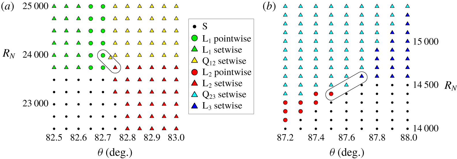
States observed in the neighbourhoods of the double-Hopf bifurcations between (a)  $\text{L}_{1}$ and
 $\text{L}_{2}$, and (b)
 $\text{L}_{2}$ and
 $\text{L}_{3}$. The symbols are loci of stable states: steady state S, limit cycles
 $\text{L}_{1}$,
 $\text{L}_{2}$ and
 $\text{L}_{3}$ and mixed-mode quasiperiodic states
 $\text{Q}_{12}$ and
 $\text{Q}_{23}$; their spatio-temporal symmetry types are also indicated.

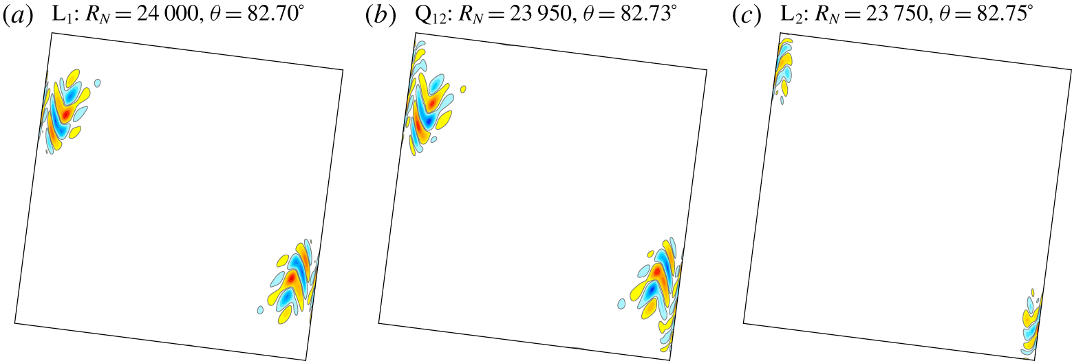
Snapshots of the perturbation vorticity in the neighbourhood of the double-Hopf bifurcation point shown in figure 14(a): (a)  $\text{L}_{1}$, (b)
 $\text{Q}_{12}$ and (c)
 $\text{L}_{2}$, at
 $R_{N}$ and
 $\unicode[STIX]{x1D703}$ as indicated. See the online movie ‘Movie 3’ for an animation.

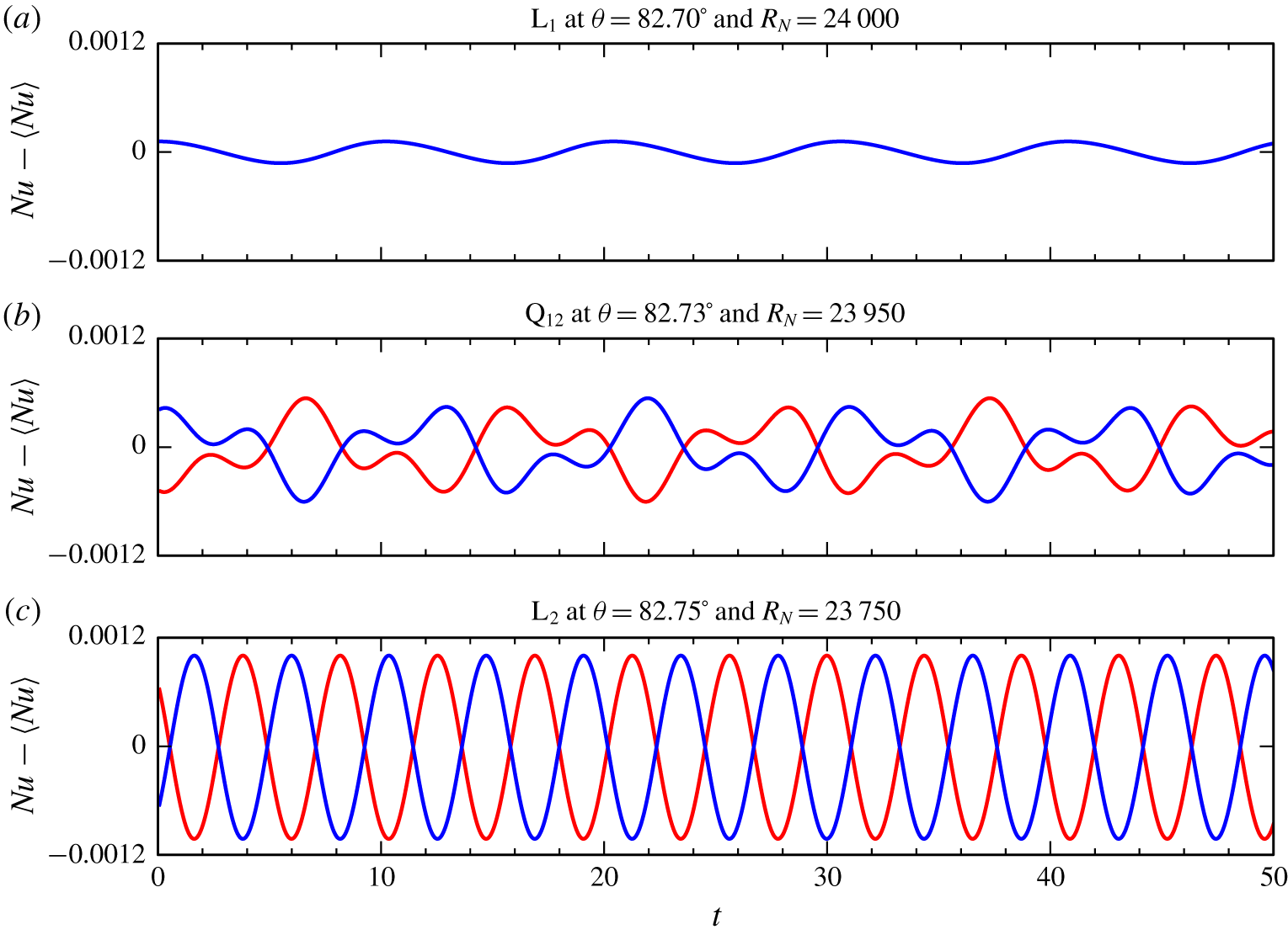
Time series of the perturbation Nusselt number on the cold wall,  $Nu_{c}-\langle Nu_{c}\rangle$ (blue), and on the hot wall
 $Nu_{h}-\langle Nu_{h}\rangle$ (red), for the flows shown in figure 15 in the neighbourhood of a double-Hopf bifurcation.

As  $\unicode[STIX]{x1D703}$ is increased beyond approximately
 $82.75^{\circ }$, the primary instability of the steady state S switches from a supercritical Hopf bifurcation spawning
 $\text{L}_{1}$ to a different supercritical Hopf bifurcation spawning
 $\text{L}_{2}$. The two limit cycles,
 $\text{L}_{1}$ and
 $\text{L}_{2}$, differ in a number of ways;
 $\text{L}_{2}$ has a higher frequency than
 $\text{L}_{1}$ which increases rapidly with increasing
 $\unicode[STIX]{x1D703}$ (see figure 8). The propagation direction (phase velocity) of the perturbation vorticity oscillations of
 $\text{L}_{2}$ is opposite that of
 $\text{L}_{1}$. For
 $\text{L}_{2}$, the small opposite-signed cells in the perturbation vorticity cycle up (down) the hot (cold) wall, and they are localized much closer to the wall and very close to the corners of the cavity. At
 $\unicode[STIX]{x1D703}\approx 82.75^{\circ }$ and
 $R_{N}\approx 23\,800$, the two Hopf bifurcation curves cross at a codimension-2 double-Hopf bifurcation. The ratio of the
 $\text{L}_{1}$ and
 $\text{L}_{2}$ frequencies near the double-Hopf bifurcation is close to 3 : 7, which is not close to a strong resonance. Figure 14(a) is a regime diagram in the neighbourhood of the double-Hopf bifurcation between
 $\text{L}_{1}$ and
 $\text{L}_{2}$, showing the loci of stable states. In this neighbourhood,
 $\text{L}_{2}$ is setwise invariant and
 $\text{L}_{1}$ is pointwise invariant, although for slightly lower
 $\unicode[STIX]{x1D703}$,
 $\text{L}_{1}$ is setwise invariant. Also in this neighbourhood, there is a stable quasiperiodic state
 $\text{Q}_{12}$ which bifurcates via a Neimark–Sacker bifurcation from either
 $\text{L}_{1}$ or
 $\text{L}_{2}$, depending on the path taken in
 $(\unicode[STIX]{x1D703},R_{N})$-space;
 $\text{Q}_{12}$ is stable in the neighbourhood of the double-Hopf point shown, and the limit cycles lose stability at the Neimark–Sacker bifurcations. Figure 15 shows snapshots of
 $\text{L}_{1}$,
 $\text{L}_{2}$ and
 $\text{Q}_{12}$ very close to the double-Hopf point (the three states encircled in figure 14a). The online movie ‘Movie 3’ provides an animation of the three states. It is apparent that
 $\text{Q}_{12}$ is essentially a linear combination of
 $\text{L}_{1}$ and
 $\text{L}_{2}$. With the frequencies of
 $\text{L}_{1}$ and
 $\text{L}_{2}$ being close to a rational ratio,
 $\text{Q}_{12}$ is close to being a locked periodic solution on a two-torus. This is also apparent from the time series of the perturbation Nusselt numbers (
 $Nu-\langle Nu\rangle$, where
 $\langle \cdot \rangle$ indicates time average) shown in figure 16, which also indicates that
 $\text{L}_{1}$ is pointwise invariant and both
 $\text{L}_{2}$ and
 $\text{Q}_{12}$ are setwise invariant. Setwise invariance for non-periodic states, such as
 $\text{Q}_{12}$, means that applying
 ${\mathcal{C}}$ at any point in time results in the same state at some later time. If an unsteady state is neither pointwise nor setwise invariant, applying
 ${\mathcal{C}}$ results in a different (conjugate) state.
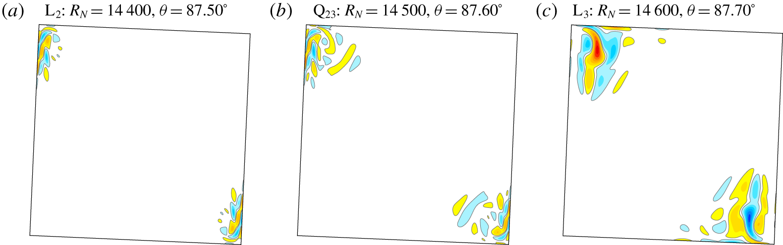
Snapshots of the perturbation vorticity for observed states in the neighbourhood of the double-Hopf point of  $\text{L}_{2}$ and
 $\text{L}_{3}$: (a)
 $\text{L}_{2}$, (b)
 $\text{Q}_{23}$ and
 $(c)$
 $\text{L}_{3}$, at
 $R_{N}$ and
 $\unicode[STIX]{x1D703}$ as indicated and
 $\unicode[STIX]{x1D703}$ as indicated. See online movie ‘Movie 4’ for an animation.

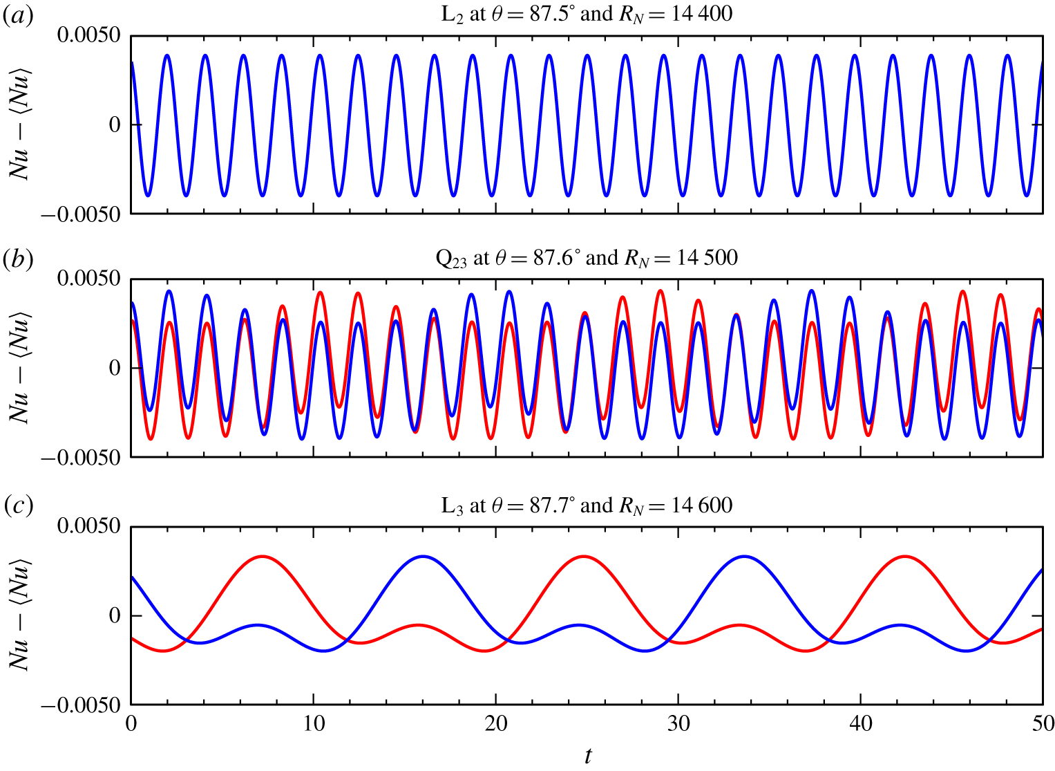
Time series of the perturbation Nusselt numbers on the cold wall  $Nu_{c}-\langle Nu_{c}\rangle$ (blue) and the hot wall
 $Nu_{h}-\langle Nu_{h}\rangle$ (red) for the flows shown in figure 17 in the neighbourhood of a double-Hopf bifurcation.

Increasing the tilt angle beyond  $\unicode[STIX]{x1D703}\approx 87.6^{\circ }$, the primary instability of the steady state S switches to a Hopf bifurcation spawning another limit cycle
 $\text{L}_{3}$. Figure 14(b) is a regime diagram in the neighbourhood of the double-Hopf bifurcation between
 $\text{L}_{2}$ and
 $\text{L}_{3}$, where again there exists a stable quasiperiodic mixed mode
 $\text{Q}_{23}$. Snapshots of the perturbation vorticity of
 $\text{L}_{2}$,
 $\text{Q}_{23}$ and
 $\text{L}_{3}$ in the neighbourhood of the double-Hopf bifurcation (the three states encircled in figure 14b) are shown in figure 17 and they are animated in the online movie ‘Movie 4’. Again, it is clearly evident that
 $\text{Q}_{23}$ is a mixed mode of
 $\text{L}_{2}$ and
 $\text{L}_{3}$;
 $\text{L}_{2}$ has the same local behaviour as the example
 $\text{L}_{2}$ shown at lower
 $\unicode[STIX]{x1D703}$ in figure 15, albeit localized much closer to the two corners at
 $(x,z)=(\pm 0.5,\pm 0.5)$. However, whereas the one shown in figure 15 is setwise invariant, the
 $\text{L}_{2}$ in figure 17 is pointwise invariant. The mixed-mode
 $\text{Q}_{23}$ is also setwise invariant. These invariances are evident from the time series of the perturbation Nusselt numbers shown in figure 18.
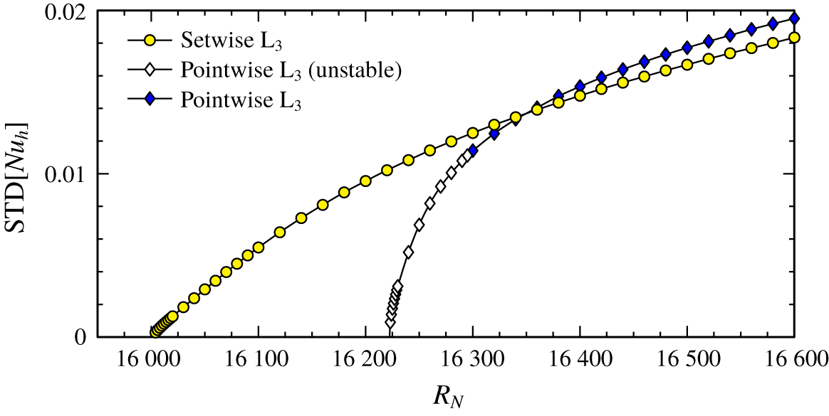
Bifurcation diagram for  $\unicode[STIX]{x1D703}=90^{\circ }$ as the buoyancy number
 $R_{N}$ is varied.

Figure 19 is a bifurcation diagram for  $\unicode[STIX]{x1D703}=90^{\circ }$, using the standard deviation in the perturbation Nusselt number
 $Nu_{h}$ at the hot wall as a measure of oscillation amplitudes. The steady state S loses stability via a supercritical symmetry-breaking Hopf bifurcation at
 $R_{N}\approx 16\,004$, giving birth to a setwise invariant
 $\text{L}_{3}$ limit cycle. Restricting the simulations to the
 ${\mathcal{C}}$-invariant subspace, S loses stability at the slightly higher
 $R_{N}\approx 16\,223$ at a supercritical Hopf bifurcation that spawns the pointwise invariant
 $\text{L}_{3}$. In the full space, this
 $\text{L}_{3}$ is unstable near onset (as it bifurcates supercritically from an unstable S), but regains stability at
 $R_{N}\approx 16\,300$ (presumably via a Neimark–Sacker bifurcation that spawns an unstable quasiperiodic state). These results are consistent with what was found by Le Quéré & Behnia (Reference Le Quéré and Behnia1998), Xin & Le Quéré (Reference Xin and Le Quéré2006).
5 Discussion and conclusions
The flow in a differentially heated tilted square container, with two opposite thermally conducting walls and two opposite insulated walls presents a non-intuitively obvious connection between two well known but completely different states. When the tilt angle  $\unicode[STIX]{x1D703}=0^{\circ }$ (the top wall is the hot one), the state is static with a stable linear stratification, regardless of how strong the stratification is (as quantified by the buoyancy number
 $R_{N}$ giving the balance between buoyancy and viscous effects). At the other extreme, with the cavity tilted at
 $\unicode[STIX]{x1D703}=90^{\circ }$, above a critical
 $R_{N}$ there is an unsteady flow that quickly becomes complicated with increasing
 $R_{N}$ (e.g. Paolucci & Chenoweth Reference Paolucci and Chenoweth1989). What we have addressed is what happens for intermediate tilt angles. What makes this problem non-intuitive is that small
 $R_{N}$ could be interpreted as implying large dissipative viscous effects, so that steady states are to be expected, while on the other hand large
 $R_{N}$ could imply a strong stable stratification, which should also be stabilizing. Yet, above a critical
 $\unicode[STIX]{x1D703}$-dependent
 $R_{N}$ there is instability. The competition between these two normally stabilizing effects (viscous dissipation and stable stratification) plays out in the boundary layers.
While the competition is in the boundary layers, the cause of the instability is not entirely local. The boundary layer flows on the conducting and insulated walls are not balanced, and this leads to the emission of horizontal shear layers from the corners where they meet. These shear layers are horizontal because the flow below the critical  $R_{N}$ is steady and stably stratified. They impinge on the wall opposite the corner. If that wall is insulated (this is so when
 $\unicode[STIX]{x1D703}<45^{\circ }$), the flow remains steady (at least for
 $R_{N}\leqslant 10^{6}$, the largest value considered). For
 $\unicode[STIX]{x1D703}>45^{\circ }$, the wall of impingement is conducting, and the strong boundary layer on it is locally perturbed by the shear layer. Below the critical
 $R_{N}$ the flow remains steady, but for larger
 $R_{N}$ unsteadiness ensues. For
 $45^{\circ }<\unicode[STIX]{x1D703}\lesssim 83^{\circ }$, the limit cycle
 $\text{L}_{1}$ has a frequency that is close to the buoyancy frequency, decreasing with increasing
 $\unicode[STIX]{x1D703}$, and the local unsteady perturbations emit internal waves when the frequency is less than the buoyancy frequency. These internal waves are very weak. Their associated vorticity is a fraction of a per cent of the vorticity in the impinging shear layers, and are of no dynamical consequence. The internal waves are a symptom of, rather than the cause of the instability.
The nature of the instability changes for  $83^{\circ }\lesssim \unicode[STIX]{x1D703}\lesssim 88^{\circ }$. The horizontal shear layers are now very close to the insulated walls and are absorbed into their boundary layers. Now, the boundary layer flows on the conducting walls are much faster than at lower
 $\unicode[STIX]{x1D703}$ and they impinge into the corner regions, leading to a corner-localized instability. The resulting limit cycle
 $\text{L}_{2}$ has a higher frequency than
 $\text{L}_{1}$, and larger than the buoyancy frequency. For
 $88^{\circ }\lesssim \unicode[STIX]{x1D703}\lesssim 90^{\circ }$, the instability is the familiar instability of the laterally heated cavity flow, with limit cycle
 $\text{L}_{3}$ at onset. Now, the fast boundary layer flows along the conducting walls hit the corners and rebound back into the interior, advecting hotter (colder) fluid from the top (bottom) insulated wall boundary layers, resulting in local convectively unstable flow regions. The limit cycle
 $\text{L}_{3}$ has a low frequency, approximately 30 % of the buoyancy frequency in the bulk and, as with
 $\text{L}_{1}$, weak internal waves are driven.
Acknowledgements
We thank ASU Research Computing facilities and the NSF XSEDE programme for providing compute resources, and K. Wu for the original code. This research was also supported via the resources provided by the Open Science Grid (Pordes et al. Reference Pordes, Petravick, Kramer, Olson, Livny, Roy, Avery, Blackburn, Wenaus and Würthwein2007; Sfiligoi et al. Reference Sfiligoi, Bradley, Holzman, Mhashilkar, Padhi and Wurthwein2009), which is supported by the National Science Foundation award 1148698, and the US Department of Energy’s Office of Science.
Declaration of interests
The authors report no conflict of interest.
Supplementary movies
Supplementary movies are available at https://doi.org/10.1017/jfm.2019.913.