3. Results and discussion

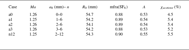
One case with only random, short-wavelength perturbations (hereafter referred to as the cylindrical case), and four cases with superimposed single-mode, long-wavelength perturbations (referred to as single-mode cases), are investigated. The initial conditions for each case are summarised in table 1. This shows that all cases are nearly identical in terms of flow parameters except for the initial interface shape. In cylindrical coordinate systems, the interface shape is described as $R=R_0 + a_0 \cos (n \theta )$ , where $a_0$ is the initial amplitude, $n$ is the azimuthal mode number, and $R_0$ is the radius of the initial interface, taken as 55 mm in this study. Case n12 exhibits the highest amplitude-to-wavelength ratio 0.048, which still corresponds to a relatively small perturbation. The Atwood number $A$ is defined as $A = (\rho _2 - \rho _1)/(\rho _2 + \rho _1)$ , where $\rho _1$ and $\rho _2$ are the gas densities outside and inside the interface, respectively. The gas enclosed by the interface is a three-component mixture of SF $_6$ , acetone vapour, and a small amount of residual air. The mass fraction of SF $_6$ is estimated using one-dimensional gas dynamics theory.

Table 1.

Initial conditions for a case without long-wavelength perturbation and cases with single-mode long-wavelength perturbation: $\textit{Ma}$ is the Mach number of the incident shock when it arrives at the interface; $a_0$ is the initial amplitude of long-wavelength perturbation; $n$ is the initial azimuthal mode number of long-wavelength perturbation; $R_0$ is the radius of initial interface; mfra(SF $_6$ ) is the SF $_6$ mass fraction; $A$ is the Atwood number; and $\chi _{\mathit{acetone}}$ is the acetone volume fraction.

Before reconstructing the scalar field, the distortion of the imaging system is corrected using a circular calibration plate. Quantitative extraction of the heavy-gas mole fraction from PLIF images accounts for both the divergence and spatial variation of the laser sheet as well as absorption losses governed by Beer’s law. The spatial intensity distribution of the laser sheet is measured by filling the test section with a uniformly mixed air–acetone mixture. Because the laser operates in burst mode, the laser-sheet profile is calibrated on a pulse-resolved basis. Although the sheet profile varies within a burst due to thermal lensing, repeated calibration experiments demonstrate that profiles corresponding to the same pulse number are highly repeatable across bursts. Accordingly, each PLIF image is corrected using the laser-sheet profile associated with the same pulse index within the burst. Assuming adiabatic mixing (Herzog et al. Reference Herzog, Ames, Noble, Oakley, Bonazza and Rothamer2019), the mole-fraction field is iteratively computed along each ray path using the equations

(3.1) \begin{equation} \xi ^r=\displaystyle {\frac {S^{f,r}}{\displaystyle { \frac{S^{f,R}}{\xi ^R}} {\frac{\sigma ^r\phi ^r}{\sigma ^R\phi ^R}} {\frac{p^rT^R}{p^RT^r}}-n_0\sigma ^r\phi ^r {\frac{T_0p^r}{T^rp_0}}\int _r^R \frac{S^f}{\phi }\,\text{d}r}}, \end{equation}

(3.2) \begin{equation} T^r=\displaystyle {\frac {\xi ^r C_{p,1}T_1+\left ( 1-\xi ^r \right ) C_{p,2}T_2}{\xi ^r C_{p,1}+\left ( 1-\xi ^r \right ) C_{p,2}}}, \end{equation}

where $\xi$ is the mole fraction of the seeded gas mixture, $S^f$ is the recorded fluorescence signal, $p$ and $T$ are the pressure and temperature, $n$ is the gas number density, $\sigma$ is the absorption cross-section, $\phi$ is the fluorescence quantum yield, and $C_{\!p}$ is the specific heat at constant pressure. The superscripts $r$ and $R$ denote local and reference positions, respectively, subscript 0 indicates the initial condition, and the overbar represents an averaged quantity. Here, $T_1$ and $T_2$ correspond to the temperatures inside and outside the interface. Because the SF $_6$ /air pair has different thermal properties, the two gases can reach different post-shock temperatures even under the present shock conditions. This, in turn, affects the acetone absorption cross-section and fluorescence quantum yield, necessitating an iterative solution of (3.1) and (3.2). Converged mole-fraction fields of the heavy gas are obtained after approximately six iterations.

Figure 2.

Schematic diagram of the region division in the PLIF processing.

Because the laser sheet enters from the side, the mole-fraction reconstruction is performed differently in the central and side regions, as illustrated in figure 2. In the central region, each ray traverses a sufficiently long path through uniformly seeded SF $_6$ before reaching the mixing layer, allowing a reference state to be defined in the pure seeded gas. Equations (3.1) and (3.2) are then solved iteratively along the ray path. In the side regions, rays pass through only a short segment of the seeded gas, and no reliable reference state is available. Owing to the weak absorption, the PLIF signal is first corrected using the transverse laser-sheet profile measured at the corresponding pulse index in a uniformly seeded calibration field. The local heavy-gas mole fraction is then estimated from the corrected intensity via a linear relationship, following the weak-absorption treatment adopted in previous RM experiments (Tomkins et al. Reference Tomkins, Kumar, Orlicz and Prestridge2008). The two reconstructions are finally blended within a narrow overlap region to obtain a continuous mole-fraction field.

Figure 3.

(a) Initial interface morphologies, and (b) the power spectra of the initial perturbations. The black line in (b) serves as a reference for a scaling law.

Figure 3(a) presents the initial interface morphologies for the cylindrical and single-mode cases. All interfaces display thin diffusion layers that are almost imperceptible, implying that initial interfacial mixing between the two gases is very limited. Also, the single-mode interfaces exhibit well-defined sinusoidal shapes. Note that the small-scale defects near the walls, caused by minor air entrainment, have little effect on the central region and can therefore be neglected in subsequent statistical analyses. Compared with our previous gas interfaces produced using the soap-film technique, where surface tension suppresses most high-frequency perturbations, the present interfaces preserve randomly distributed short-wavelength disturbances superimposed on the regular long-wavelength modulations. To quantitatively characterise the perturbations, the isocontour at $\xi =0.5$ is extracted to represent the interface. Because this contour is single-valued, a spatial Fourier transform can be applied to obtain the initial perturbation power spectra, as shown in figure 3(b).

The power spectra show that compared with the cylindrical case, the single-mode interfaces exhibit distinct low-wavenumber peaks associated with the imposed long-wavelength structures. For cases a1, a2 and a3 with mode number $n=6$ , the spectral peak appears at 17.5 m $^{-1}$ , while case n12 with $n=12$ peaks at 35 m $^{-1}$ , satisfying the expected doubling relation. Beyond the dominant peaks, all single-mode cases display broadband low-energy perturbations following a $k^{-4/3}$ scaling, similar to the high-wavenumber behaviour in the cylindrical case. This consistency indicates that although the short-wavelength components are not actively controlled, the shared fabrication process ensures similar spectral features across cases. Therefore, variations in the scalar energy spectra observed later can be attributed to the interaction between long-wavelength structures and the converging shock, as well as differences in energy transfer associated with interface morphology.

Figure 4.

Time-resolved PLIF mole-fraction fields for all cases: II indicates initial interface; SI indicates shocked interface; TS indicates transmitted shock; RTS indicates reflected transmitted shock; RI indicates reshocked interface. The time origin is $t=0$ at first shock–interface contact.

Temporal evolutions of the mole-fraction distributions for all cases are presented in figure 4. Each column in figure 4 shows a time-resolved sequence of PLIF diagnostics capturing the evolution of the converging RM instability, from linear growth through nonlinear development to turbulent mixing. The time origin ( $t=0$ ) is defined as the moment when the incident shock wave first interacts with the interface. The first row displays the interface prior to shock arrival, while the second row shows the post-shock state. Compared to previous studies (Weber et al. Reference Weber, Haehn, Oakley, Rothamer and Bonazza2014; Mohaghar et al. Reference Mohaghar, Carter, Musci, Reilly, McFarland and Ranjan2017), the pre-reshock interface in the present experiments exhibits reduced diffusivity, while retaining rich small-scale structures that are conducive to turbulent transition. When the transmitted shock reaches the centre of convergence, it generates an outward-propagating reflected shock that subsequently reshocks the interface. During reshock, the interface is temporarily compressed, and the amplitude of the perturbations is reduced to a minimum. However, this phase is short-lived. In the cylindrical case (case a0), short-wavelength perturbations grow rapidly following reshock, initiating an early transition to turbulence at approximately $t = 0.35$ ms. In the single-mode case (case a1), both short- and long-wavelength perturbations increase continuously, accompanied by a clear phase inversion, in which the azimuthal positions of spikes and bubbles are reversed. This results in the emergence of a large-scale azimuthal pattern of interleaving spikes and bubbles. For cases a2 and a3, the post-reshock interfaces exhibit similar behaviour: prominent spikes rapidly penetrate outwards, and exit the observable region of the test section, thereby limiting the number of recorded frames. In contrast, the interface in case n12 does not extend beyond the field of view but exhibits more intense mixing. The close spatial proximity between spikes and bubbles in case n12 enhances their mutual interaction, strongly stretching the interface and promoting fragmentation of large-scale structures.

Figure 5.

Trajectories of the interface and shock waves: IS indicates incident shock; RS indicates first reflected shock; TS indicates first transmitted shock; RTS indicates reflected transmitted shock; TS $_2$ indicates second transmitted shock. The interface position is defined by the azimuthal average $\langle \xi \rangle =0.5$ . Vertical lines mark incident shock and reshock.

An $r$ – $t$ diagram illustrating the trajectories of interfaces and shock waves is presented in figure 5. The shock trajectories, obtained from a one-dimensional gas dynamics calculation, show good agreement with the experimentally observed wave motions. The interface position is extracted from the PLIF-derived mole-fraction fields using the azimuthally averaged condition $\langle \xi \rangle = 0.5$ . The azimuthal averaging is defined as

(3.3) \begin{equation} \left \langle \xi \right \rangle ={\frac {1}{r\left ( \theta _2-\theta _1 \right )}}\int _{\theta _1}^{\theta _2}{\xi r\,\text{d}\theta }, \end{equation}

where $r$ denotes the local radius, and $\theta$ is the azimuthal angle, ranging from $\theta _1 = 0$ to $\theta _2 = \pi$ . The interface trajectories for all cases closely coincide, confirming that the initial conditions (e.g. shock strength and fluid properties) are nearly identical, with differences only in the imposed interface perturbation. Following incident shock impact, the interface moves inwards with initial velocity approximately 110 m s $^{-1}$ . As the shock focuses at the geometrical centre, the adverse pressure gradient along the radial direction causes significant deceleration of the interface. After reshock, all cases again exhibit similar interface velocities, followed by further deceleration. From an RT instability perspective, inward deceleration tends to stabilise the interface, whereas outward deceleration following reshock promotes instability and mixing. At later times, the interface undergoes oscillations in radial direction induced by reverberating waves, during which case-dependent discrepancies in interface position begin to emerge. These differences arise primarily from asymmetric interfacial deformation: cases with larger initial amplitudes or higher azimuthal mode numbers tend to produce more inwardly displaced interfaces. Overall, the $r$ – $t$ diagram highlights the dominance of shock-induced acceleration histories in shaping the interfacial evolution, while also demonstrating how subtle variations in initial geometry can lead to diverging flow behaviour at later stages. Such observations underscore the importance of initial conditions in determining the onset and development of RT-type mixing in converging shock-driven flows.

Figure 6.

(a) Time variations of the perturbation amplitudes for single-mode cases. Here, $a$ is the amplitude of the interface, normalised by the initial amplitude $a_0$ . The dimensionless time is expressed as $\tau =t V_0 / R_0$ , where $t$ is time (ms), $V_0$ is the initial interface velocity induced by the incident shock, and $R_0$ is the initial interface position. (b) Temporal variations of the mixing width.

Prior to reshock, the interfaces in the single-mode cases exhibit well-defined peaks and troughs. For the single-mode cases, the imposed dominant perturbation remains approximately sinusoidal before reshock, so its amplitude is measured directly from the PLIF images and is defined as one-half of the visual mixing width of the dominant mode. This allows direct comparison of perturbation growth with classical theoretical models developed for converging RM instability. For cylindrical single-mode perturbation growth, a modified Bell model, referred to as the Bell-RTS model, was proposed by Ding et al. (Reference Ding, Si, Yang, Lu, Zhai and Luo2017) to incorporate RM impulsive growth, Bell–Plesset geometric effect and RT effect:

(3.4) \begin{equation} a( t ) -a_0=\dot {a}_0r_{0}^{2}\int _{t_{0}^{+}}^t{\frac {1}{r^2}\,\mathrm{d}t+\left ( nA-1 \right )}\int _{t_{0}^{+}}^t{\left ( \frac {1}{r^2}\int _{t_{0}^{+}}^t{ar\ddot {r}\,\mathrm{d}t^{\prime }} \right ) \mathrm{d}t}, \end{equation}

where $a$ is the perturbation amplitude, $\dot {a}_0$ is the post-shock initial growth rate, $r$ is the time-dependent radius, and $n$ is the azimuthal mode number. As shown in figure 6(a), the early-time growth of interface amplitudes in the single-mode cases collapses onto a common trend when appropriately normalised, and is well captured by the Bell-RTS model. In particular, the experimental data strongly support the theoretically predicted reduction of amplitude growth rate due to RT stabilisation effects.

The evolution of the mixing layer width $h$ is presented in figure 6(b), where $h$ is defined by the radial distance between two scalar thresholds:

(3.5) \begin{equation} h=r_{\left \langle \xi \right \rangle =0.05}-r_{\left \langle \xi \right \rangle =0.95}, \end{equation}

with $r_{\langle \xi \rangle = 0.05}$ and $r_{\langle \xi \rangle = 0.95}$ representing the mean radii of the spike and bubble fronts, respectively, based on azimuthally averaged mole-fraction profiles. Following the impact of incident shock, case n12 develops the widest mixing region, whereas case a0 remains the narrowest, in positive correlation with the initial amplitude-to-wavelength ratio. Following reshock, the mixing width first suffers a sudden drop due to shock compression, then presents a long period of quasi-linear growth with a higher growth rate. The post-reshock growth can be evaluated using the empirical linear model by Mikaelian (Reference Mikaelian1989):

(3.6) \begin{equation} \frac {\mathrm{d}h}{\mathrm{d}t}=C_{\!M}\,\Delta V\left | A_{r}^{+} \right |\!, \end{equation}

where $\Delta V$ is the velocity jump across the interface after reshock, $A_r^+$ is the post-reshock Atwood number, and $C_{\!M}$ is an empirical coefficient. While $C_{\!M}$ is typically $0.28{-} 0.39$ for planar reshocked RM flows (Leinov et al. Reference Leinov, Malamud, Elbaz, Levin, Ben-Dor, Shvarts and Sadot2009), values obtained from the current experiments are significantly higher: 0.99, 0.97, 1.02, 1.23 and 1.09 for cases a0, a1, a2, a3 and n12, respectively. This enhancement suggests that geometric convergence significantly accelerates scalar mixing relative to planar configurations. The present growth rates are close to those reported in three-dimensional simulations of converging RM turbulence in unconstrained domains by Li et al. (Reference Li, Fu, Yu and Li2021). This agreement suggests that the limited height of the test section does not materially affect the overall growth of the mixing layer. Although the confined dimension may eventually restrict the growth of the largest transverse structures at sufficiently late times, no such confinement effect is evident in the present measurements.

The elevated growth rates after reshock are primarily driven by RT instability arising from the deceleration of the outward-moving interface, as evidenced by the interface dynamics in figure 5. Moreover, the relatively small variations in $C_{\!M}$ across the cases, except for the slightly larger value in case a3, imply that reshock largely suppresses differences originating from the initial interface morphology. At later times, the mixing width growth tends to saturate, and the presence of reverberating waves introduces oscillatory behaviour in the width evolution. These observations highlight that while early-time evolution is strongly influenced by initial amplitude and wavelength, the late-stage turbulent mixing is predominantly governed by reshock dynamics and RT instability that is unique to converging RM turbulence. The enhanced mixing efficiency in cylindrical geometry further underscores the critical influence of geometric effects on RM turbulence.

Figure 7.

Temporal evolution of mixedness $\varPsi$ for all cases (definition given in (3.7)).

The degree of molecular mixing is a key metric for quantifying the homogeneity of the scalar field within the mixing layer, particularly reflecting the interpenetration and diffusion of the fluids. In the present study, the mixing degree is defined by the normalised mixed mass introduced by Zhou, Cabot & Thornber (Reference Zhou, Cabot and Thornber2016):

(3.7) \begin{align} \varPsi =\frac {\int {\left \langle \rho \xi \left ( 1-\xi \right ) \right \rangle \text{d}r}}{\int {\left \langle \rho \right \rangle \left \langle \xi \right \rangle \left \langle 1-\xi \right \rangle \text{d}r}}, \end{align}

where $\xi$ denotes the mole fraction of the heavy gas, $\rho$ is the local density, and $\langle {\cdot }\rangle$ denotes azimuthal averaging. The local density $\rho$ is evaluated from the mole-fraction field by assuming approximately uniform pressure within the thin mixing layer and applying a linear mixture relation $\rho =\rho _1'+(\rho _2'-\rho _1')\xi$ , where $\rho _1'$ and $\rho _2'$ are the post-shock densities on the light- and heavy-gas sides. A value $\varPsi = 1$ corresponds to fully homogenised molecular mixing, while $\varPsi = 0$ represents a completely unmixed, segregated interface.

As shown in figure 7, the initial values of $\varPsi$ differ across cases, reflecting variations in initial interface sharpness and fine-scale structures. Case a0 exhibits the highest initial $\varPsi$ , likely owing to the absence of long-wavelength perturbations and its relatively smooth interface, whereas single-mode cases begin with smaller $\varPsi$ values due to stronger spatial segregation. Following shock–interface interaction, perturbation growth rapidly increases the interfacial surface area, resulting in a sharp decline of $\varPsi$ to a local minimum. Subsequently, RT stabilisation due to interface deceleration reduces the growth rate of the mixing width and gradually increases $\varPsi$ , indicating progressive homogenisation. After reshock, distinct trends emerge among these cases. In case a0, $\varPsi$ shows a slight decline, suggesting that large-scale structures, such as merging bubbles, contribute more to the entrainment of unmixed fluid than to homogenisation. In contrast, the single-mode cases continue to exhibit increasing $\varPsi$ , driven by enhanced small-scale mixing during phase inversion and the nonlinear growth of perturbations. The development of azimuthally distributed spikes and bubbles facilitates localised turbulent transitions, which significantly promote molecular mixing. Eventually, $\varPsi$ saturates in the range $0.8{-}0.9$ for cases a0, a1 and n12, consistent with efficient turbulent homogenisation. In contrast, lower saturation values of $\varPsi$ are observed in cases a2 and a3, attributed to the dominance of large-scale structures with insufficient fragmentation. As is evident from figure 4, spike regions tend to exhibit greater mixing homogeneity than bubble regions, whereas bubbles often maintain sharper gradients and coherent morphology. These observations underscore the asymmetric role of spike and bubble dynamics in controlling the scalar homogenisation process. The variations in mixing across cases highlight the sensitivity of scalar-field development to both the initial perturbations and the evolution of large-scale coherent structures. This reinforces the importance of modal content and geometric effects in determining the efficiency of turbulent mixing in converging RM flows.

Figure 8.

Dissipation rate field overlaid on the mole-fraction field.

The scalar dissipation rate, defined as $\chi = D\, \boldsymbol{\nabla }\xi \boldsymbol{\cdot }\boldsymbol{\nabla }\xi$ , serves as a key indicator of local mixing intensity in turbulent flows, capturing both the sharpness of scalar gradients and the efficiency of molecular diffusion (Sreenivasan Reference Sreenivasan1991; Warhaft Reference Warhaft2000; Dimotakis Reference Dimotakis2005). Here, $\xi$ denotes the mole fraction of the heavy gas, and the diffusion coefficient $D$ is estimated using the empirical model proposed by Ramshaw (Reference Ramshaw1990). The evolutions of dissipation rate fields for all cases are presented in figure 8, superimposed on the corresponding mole-fraction distribution to highlight the spatial structure of dissipation relative to scalar features. At early times, prior to and shortly after the incident shock, the scalar dissipation field is primarily localised along the perturbed interface, and exhibits elongated structures aligned with the interface direction. These features reflect the intense scalar gradients formed by shock compression and baroclinic generation. As the reflected shock impinges on the interface, the scalar field rapidly evolves into smaller scales, and the dissipation field becomes increasingly fragmented and disordered, indicating enhanced mixing and a transition towards local isotropy.

In the single-mode cases, the dissipation is initially concentrated along the arc-shaped interface, and progressively spreads into the interior of the mixing layer. The orientation of dissipation structures gradually shifts from being tangential to the interface to a more radial and scattered distribution, consistent with the expansion of the mixing layer and the onset of small-scale turbulence. Despite the dominance of large-scale spike and bubble structures in the single-mode configuration, numerous fine-scale, randomly distributed dissipative features persist within the mixing layer. These structures, rooted in the initial multi-mode, short-wavelength perturbations, significantly enhance scalar gradients and support the turbulent cascade. Notably, in the well-mixed case (n12), the dissipation structures diminish within the mixing layer interior at later times, while becoming more prominent near the mixing boundaries. This redistribution suggests a gradual decay of scalar gradients in the core region, and reflects the decreasing internal mixing rate as the scalar field approaches a more homogeneous state. Note that the measured dissipation is affected by the finite spatial resolution of the PLIF system. With image resolution 0.17 mm per pixel and laser-sheet thickness approximately 0.5 mm, scalar gradients at smaller scales are smoothed by optical blur and pixel averaging. As a result, the finest gradient structures are not fully resolved, and the measured $\chi$ should be regarded as a lower-bound estimate of the true scalar dissipation, especially after reshock when sharp scalar gradients become more abundant.

Figure 9.

Evolution of the spatially averaged dissipation rate ( $\bar {\chi }$ ) and mixing area ( $S$ ). Hollow symbols represent $\bar {\chi }$ , while solid symbols represent $S$ .

To assess the global evolution of dissipation, the area-averaged scalar dissipation rate is computed as $\bar {\chi } = \iint \chi r\,\text{d}r\text{d}\theta / S$ , where the mixing area $S$ is defined as the region satisfying $0.05 \lt \xi \lt 0.95$ , i.e.

(3.8) \begin{equation} S=\iint {H\left ( \left | \xi -0.5 \right |-0.45 \right ) r\,\mathrm{d}r \mathrm{d}\theta }, \end{equation}

with $H({\cdot })$ denoting the Heaviside function. As shown in figure 9, the temporal evolution of $\bar {\chi }$ is surprisingly consistent across all cases, regardless of their initial perturbation spectra. This result suggests that while the shape of the initial interface significantly affects the degree of mixing, the overall rate at which scalar dissipation is generated is less sensitive to such differences, indicating a form of dynamical convergence in turbulent scalar transport. Following the passage of the incident shock, the mixing layer expands slowly and remains weakly turbulent. During this period, concentration gradients weaken, resulting in a rapid decay of $\bar {\chi }$ at average rate $-8.5 \times 10^3 \ \mathrm{s}^{-2}$ . Following reshock, however, intense straining and stretching induced by shock-driven vortical structures substantially amplify the scalar gradients, leading to a sharp increase in $\bar {\chi }$ at average rate $251.2 \ \mathrm{s}^{-2}$ up to approximately 0.75 ms. As local turbulent transitions mature and energy cascades to smaller scales, the scalar field becomes increasingly homogenised, and dissipation subsequently decays again at a slower rate $-135.8 \ \mathrm{s}^{-2}$ . In the late-time regime, case n12 maintains the largest mixing area due to its broad initial perturbation spectrum and intense post-reshock activity. In contrast, cases a1, a2 and a3 achieve smaller yet comparably sustained mixing area growth, while the cylindrical case a0 stagnates. These trends imply that although interface geometry can delay or accelerate the onset of mixing, the fundamental dissipation dynamics within converging RM flows ultimately exhibit robust statistical behaviour once turbulent mixing occurs. This suggests a robust trend consistent with universality hypotheses, although further collapse using the convergence ratio is needed.

Figure 10.

(a) Example material lines (case n12) at contour levels $\xi \in \{0.1,\,0.2,\ldots ,0.9\}$ . (b) Total contour length $L$ at $\xi =0.1$ (spike) and $\xi =0.9$ (bubble), normalised by the unperturbed semi-perimeter $L_0$ .

The evolution of material interfaces and their geometric deformation is a key feature in scalar mixing processes. In this regard, the interface contour lines and their corresponding stretching lengths provide useful diagnostics of morphological complexity. Figure 10(a) presents material lines for case n12, extracted from the mole-fraction field at contour levels ranging from $\xi =0.1$ to $\xi =0.9$ in increments of 0.1. Contours near $\xi =0.1$ are typically associated with spike fronts (heavy gas penetrating into the light gas), while those near $\xi =0.9$ represent bubble fronts (light gas rising into the heavy gas). The temporal evolution of the total length of selected contour lines at $\xi =0.1$ and $\xi =0.9$ is shown in figure 10(b). To facilitate comparison across different stages, the contour length $L$ is normalised by the semi-perimeter $L_0$ of the unperturbed interface at each time. Following the incident shock compression, the interface initially contracts but quickly elongates due to perturbation growth. When RT stabilisation occurs during inward deceleration, the elongation rate slows down and eventually reverses. This behaviour is consistent with the observed stagnation in the growth of the mixing width. After reshock, the contour lengths associated with both spikes and bubbles increase sharply, particularly for the spike side, where exponential growth persists over approximately 0.3 ms. This behaviour echoes findings from earlier numerical and experimental studies of shock-accelerated gas cylinders, which reported exponential growth of material line lengths of the form $L(t)/L(0) = A\exp (\lambda t/t_0)$ , with a typical stretching exponent $\lambda \approx 0.025$ (Yang, Kubota & Zukoski Reference Yang, Kubota and Zukoski1993; Kumar et al. Reference Kumar, Orlicz, Tomkins, Goodenough, Prestridge, Vorobieff and Benjamin2005). The fitted exponents are obtained from the $\xi = 0.1$ isocontour on the spike side, which shows more pronounced post-reshock stretching. In the present study, due to the different normalisation and initial configuration, larger fitted exponents are obtained: $\lambda = 0.64$ , $0.57$ , $0.62$ , $0.62$ and $0.67$ for cases a0, a1, a2, a3 and n12, respectively. The similarity in $\lambda$ across cases suggests a robust exponential stretching regime, governed primarily by the shock-induced vorticity and interfacial shear.

As the flow evolves, the divergence in stretching behaviour becomes more pronounced. This divergence can be traced back to the initial perturbation spectra shown in figure 3(b). Cases a1, a2 and a3 all share the same dominant low-wavenumber peak at $n=6$ , therefore their contour-length evolutions remain relatively close to one another. The differences among these three cases mainly arise from the different amplitudes of this same large-scale mode. By contrast, case n12 is characterised by a dominant peak at $n=12$ , which corresponds to a shorter initial wavelength and a smaller spacing between adjacent spikes and bubbles. This initial spectral shift promotes stronger interface folding and stretching, and therefore leads to the largest contour length. In the late-time regime, the stretching length of single-mode cases continues to increase, whereas the cylindrical case (a0) shows a slight decline due to the progressive homogenisation of the scalar field. A notable asymmetry is also observed between the spike and bubble sides: the stretching lengths of bubble contours remain significantly smaller and plateau beyond 1 ms, while spike contours continue to elongate. This asymmetry indicates that turbulent mixing is more vigorous near the lighter (air) side than in the heavier (SF $_6$ ) region. In a broader context, the exponential elongation of material interfaces serves as a precursor to the onset of fine-scale turbulent structures. The similar exponents across cases suggest late-stage stretching dynamics that are broadly similar within experimental scatter, rather than demonstrably universal. These findings suggest that interface stretching can be a reliable predictor of transition and small-scale generation in converging RM flows.

As an intrinsically unsteady phenomenon, RM turbulence lacks a universally accepted temporal marker for the onset of turbulent transition. In particular, for single-mode cases, the imposed long-wavelength perturbations generate large-scale azimuthal spike-and-bubble structures that break planar symmetry, such that no quasi-isotropic plane emerges at the mixing-layer centre as in the random perturbation case, thereby complicating the definition of Reynolds number and other turbulence statistics based on planar averaging. As a result, conventional analyses based on Reynolds number and characteristic turbulent scales become inapplicable for characterising the onset of turbulence. In such scenarios, the fractal dimension of scalar interfaces offers a robust, geometry-independent metric for assessing the complexity and scale-invariance of the flow. Theoretical analyses by Sreenivasan, Ramshankar & Meneveau (Reference Sreenivasan, Ramshankar and Meneveau1989) demonstrated that the onset of turbulence in passive scalar fields is accompanied by the emergence of a fractal dimension $D_{\!F} = 7/3$ , underpinned by the requirement for scale-independent flux through isoconcentration surfaces. This threshold aligns with the turbulent transition criterion suggested by Dimotakis (Reference Dimotakis2000), which correlates the scalar interface geometry with a critical Reynolds number of the order of $10^4$ . In laser-sheet diagnostic studies of shock-driven gas curtains and boundary layers (Vorobieff, Rightley & Benjamin Reference Vorobieff, Rightley and Benjamin1999; de Silva et al. Reference de Silva, Philip, Chauhan, Meneveau and Marusic2013), the fractal dimension $\sim1.3$ has been reported as an empirical marker for turbulent transition in two-dimensional projections.

Figure 11.

Fractal dimension $D_{\!F}$ of the $\xi =0.1$ isocontour versus time; the reshock time is indicated. For reference, the two-dimensional projection empirical threshold $D_{\!F}\approx 1.3$ is shown as a horizontal guide.

In the present study, the scalar isocontour at $\xi = 0.1$ is extracted to assess the interface complexity via the box-counting method. Square boxes of size $r$ are used to tile the scalar contour line, and the number of required boxes $N(r)$ is expected to scale as $N(r) \sim r^{-D_{\!F}}$ within a defined inertial range, where $D_{\!F}$ is the fractal dimension. Figure 11 presents the temporal evolution of $D_{\!F}$ for each case. Initially, the fractal dimension is close to 1 across all cases, consistent with the nearly smooth, low-amplitude interface geometry. After interaction with the incident converging shock, $D_{\!F}$ increases as the interface is stretched by baroclinic vorticity, then decreases transiently due to RT stabilisation caused by interface deceleration. The reshock event introduces significant complexity to the interface geometry. As shown in previous studies (Balakumar et al. Reference Balakumar, Orlicz, Tomkins and Prestridge2008b ), reshock-induced vorticity leads to more chaotic interface wrinkling and interfacial instability, thereby promoting the emergence of small-scale structures. In the present experiments, case n12 exhibits the earliest transition, with $D_{\!F}$ exceeding the empirical threshold 1.3 at approximately 0.3 ms after reshock, following a brief period of compression and interface inversion. Case a0 transitions later, at approximately 0.5 ms after reshock. This delay, compared with previous predictions based on Reynolds number scaling, may be attributed to the resolution limitations and optical blur in the current PLIF imaging system, which underestimate the contribution of small-scale structures.

In contrast, case a1 reaches the transition threshold much later, and cases a2 and a3 do not reach $D_{\!F} \geqslant 1.3$ within the observable time frame. However, this does not imply the absence of local turbulence, but rather reflects the inherently global nature of the fractal metric. Localised turbulent structures, especially around spike tips, are still evident, but they are insufficient to elevate the overall fractal dimension. These observations suggest that while fractal dimension offers a useful scalar-based indicator for global transition, it should be complemented by localised diagnostics in strongly anisotropic or spatially inhomogeneous flows. More broadly, the current findings support the use of interface geometry as a predictive tool for turbulent transition in converging RM instability flows. The consistency in fractal scaling trends across diverse initial conditions points to a universal behaviour governed by the interplay of shock-induced baroclinicity, geometric confinement, and RT stability. Future efforts integrating multi-scale imaging and velocity field diagnostics would offer a more complete picture of both global and local transition dynamics.

Figure 12.

The post-reshock scalar energy spectra of (a) case a0, (b) case a1, (c) case a2, (d) case a3 and (e) case n12.

The scalar energy spectrum characterises the distribution of scalar fluctuations across scales. The post-reshock spectra for all cases are presented in figure 12. The calculation of the scalar energy spectrum proceeds as follows. First, the mole fraction is azimuthally averaged over each radius, and the mean value is subtracted to obtain the scalar fluctuations. The scalar fluctuations are calculated by $\xi ^\ast =\xi -\langle \xi \rangle$ . Next, the scalar fluctuations for different radii are Fourier transformed and multiplied by their conjugates to calculate the scalar energy spectrum:

(3.9) \begin{equation} E(k)=F(\xi ^\ast )\,F^{\textit{conj}}(\xi ^\ast ), \end{equation}

where $F({\cdot })$ denotes the Fourier transform, and $k$ is the azimuthal wavenumber. To isolate the spectral characteristics of the most actively mixing region, the spectra are spatially averaged within the inner mixing zone, defined by the scalar variance threshold $4\langle \xi \rangle {} (1 - \langle \xi \rangle ) \geqslant 0.9$ , following the criterion proposed by Tritschler et al. (Reference Tritschler, Olson, Lele, Hickel, Hu and Adams2014). This region corresponds to the portion of the flow where the mixing is most intense and the scalar field is neither pure nor completely homogenised, thus capturing the transition scales most effectively. To quantify the intermediate-wavenumber decay, the spectral exponent for each case is determined from the post-reshock spectra at later times. The fitting is performed at two such instants using a log–log relation of the form $E(k)\sim k^{\alpha }$ . The fitting range is selected around the intermediate wavenumber $k \approx 200\ \mathrm{m}^{-1}$ to exclude both the low-wavenumber energy-containing range and the high-wavenumber range affected by finite PLIF resolution. Owing to optical blur and pixel averaging, PLIF measurements smooth the smallest scalar structures, leading to attenuation of the high-wavenumber spectral tail. The fitted slopes should therefore be interpreted within this intermediate range, where the influence of residual coherent structures and resolution-induced attenuation is relatively weak.

Case a0 provides a useful reference because its initial interface contains only random short-wavelength perturbations. Its post-reshock spectrum shows an intermediate-wavenumber decay close to $-2.3$ , which is close to the $-7/3$ scaling reported for fully three-dimensional reshocked RM turbulence by Noble et al. (Reference Noble, Ames, McConnell, Oakley, Rothamer and Bonazza2023). This behaviour differs from strictly two-dimensional turbulence, where the forward enstrophy cascade is associated with a $k^{-3}$ spectrum (Boffetta & Ecke Reference Boffetta and Ecke2012). In the present experiments, the post-reshock flow continues to generate finer scalar structures, indicating a sustained transfer towards smaller scales rather than the inverse-cascade-dominated behaviour of two-dimensional flow. This further confirms that the limited height of the test section does not fundamentally affect the growth of the mixing layer. Relative to case a0, the single-mode cases retain a stronger imprint of the imposed large-scale structure after reshock, as reflected by higher energy levels at low wavenumbers, and distinct decay rates in the intermediate-wavenumber range. For the three cases with the same dominant mode number $n=6$ (a1, a2 and a3), the spectral differences primarily reflect the effect of the initial amplitude. As the initial amplitude increases from a1 to a3, a larger fraction of scalar energy remains concentrated at large scales after reshock, and the intermediate-wavenumber decay becomes steeper. This trend is consistent with the fractal-dimension results shown in figure 11, where flows dominated by persistent large-scale structures exhibit lower interfacial complexity and delayed development of fine-scale features. Although cases a2 and a3 exhibit slopes close to $-3$ over the fitted range, this should not be interpreted as evidence of a two-dimensional turbulent state. In the present flow, a larger imposed long-wavelength amplitude enhances large-scale segregation and strengthens nonlinear entrainment, thereby retaining more scalar energy at low wavenumbers, and producing a steeper fitted decay. By contrast, case a1, with a weaker imposed long-wavelength mode, exhibits more effective transfer of scalar energy towards smaller scales, and its spectrum remains closer to that of case a0. Case n12 does not follow the same amplitude trend because its dominant mode is shifted from $n=6$ to $n=12$ . The shorter initial wavelength reduces the spacing between neighbouring spikes and bubbles, promoting stronger post-reshock interaction, merging and break-up of large-scale structures. As a result, scalar energy is transferred more efficiently towards smaller scales than in cases a2 and a3, and its spectral scaling remains closer to that of cases a0 and a1.