

INTRODUCTION
Empirical maps of schistosomiasis transmission are important tools in guiding control interventions. Usually, these maps are based on hospital records or data arising from cross-sectional epidemiological surveys carried out over a number of locations within a designated study area (Doumenge et al. Reference Doumenge, Mott, Cheung, Villenave, Chapuis, Perrin and Reaud-Thomas1987; Brooker et al. Reference Brooker, Rowlands, Haller, Savioli and Bundy2000; Brooker, Reference Brooker2007). The data are spatially correlated because common exposures influence transmission similarly at neighbouring locations. Among other factors, these common exposures include climatic and environmental features governing the survival and longevity of the intermediate host snails (Stensgaard et al. Reference Stensgaard, Jørgensen, Kabatereine, Rahbek and Kristensen2006) and proximity of human habitations to transmission sites (Booth et al. Reference Booth, Vennervald, Kenty, Butterworth, Kariuki, Kadzo, Ireri, Amaganga, Kimani, Mwatha, Otedo, Ouma, Muchiri and Dunne2004; Kitron et al. Reference Kitron, Clennon, Cecere, Gürtler, King and Vazquez-Prokopec2006). Risk maps of schistosomiasis are produced by predicting the transmission outcome at non-sampled locations. These predictions are more accurate when they are based on models relating transmission to known environmental predictors of schistosomiasis, and when they make use of the spatial correlation present in the data, which filters the noise and highlights the existing patterns. The standard regression models assume independence of the data, leading to inaccurate estimation of the precision of the parameter estimates and of the predictions when they are applied to spatially-correlated data (Cressie, Reference Cressie1991).
In this paper, we first summarize how our ability to map and predict the distribution of schistosomiasis transmission has improved as a result of advances made with Bayesian geostatistical approaches. However, research has mainly focused on mapping and prediction of prevalence data. In view of morbidity control being the declared goal of national schistosomiasis control programmes, new research is needed for modeling infection intensity data (WHO, 2002; Bergquist, Johansen and Utzinger, Reference Bergquist, Johansen and Utzinger2009). Thus far, only one attempt has been made to predict infection intensity of Schistosoma mansoni using Bayesian inference (Clements, Moyeed and Brooker, Reference Clements, Moyeed and Brooker2006b). We examine the underlying assumptions of that model, i.e. stationarity and negative binomial distribution of egg counts. We then propose an approach that might predict the infection intensity of S. mansoni more accurately; namely a Bayesian non-stationary zero-inflated (ZI) negative binomial model. We compare the performance of this model with a negative binomial and a ZI Poisson model on the basis of credible intervals of the predictive ability of the models, using an existing high-quality georeferenced database from western Côte d'Ivoire. Finally, we discuss future research directions to further improve upon the mapping of infection intensity of schistosomiasis and other tropical diseases that are often neglected.
BAYESIAN APPROACHES FOR MAPPING AND PREDICTING SCHISTOSOMIASIS
Spatial geostatistical models introduce at each observed location an additional parameter, the so-called random effect, and build spatial correlation on the distribution of the random effects. The latter is done by assuming that the distribution arises from a multivariate normal distribution with correlation matrix often to be a parametric decreasing function of distance between any pair of locations. Fitting these models, however, is not straightforward, which is illuminated on the following grounds. First, the models include a large number of parameters, proportional to the number of observed locations. Second, computational challenges arise in relation to the large correlation matrices. Bayesian formulation of these models (Diggle, Moyeed and Tawn, Reference Diggle, Moyeed and Tawn1998), facilitates parameter estimation via Markov chain Monte Carlo (MCMC) simulation methods. The availability of software for fitting these models, although for a relatively small number of locations (Lunn et al. Reference Lunn, Thomas, Best and Spiegelhalter2000), together with the earlier established geographical information system (GIS) software and remote sensing (RS) tools enabled spatial analyses of cross-sectional prevalence data and the generation of model-based schistosomiasis risk maps (Raso et al. Reference Raso, Matthys, N'Goran, Tanner, Vounatsou and Utzinger2005, Reference Raso, Vounatsou, Singer, N'Goran, Tanner and Utzinger2006a; Yang et al. Reference Yang, Vounatsou, Zhou, Tanner and Utzinger2005a; Clements et al. Reference Clements, Lwambo, Blair, Nyandindi, Kaatano, Kinung'hi, Webster, Fenwick and Brooker2006a, Reference Clements, Brooker, Nyandindi, Fenwick and Blair2008; Beck-Wörner et al. Reference Beck-Wörner, Raso, Vounatsou, N'Goran, Rigo, Parlow and Utzinger2007; Brooker and Clements, Reference Brooker and Clements2009). These risk maps, emphasizing areas where the prevalence of schistosome infections is higher relative to other locations, are useful tools for spatial targeting of control interventions and to enhance cost-effectiveness (Brooker et al. Reference Brooker, Kabatereine, Fleming and Devlin2008, Reference Brooker, Gyapong, Kabatereine, Stothard and Utzinger2009).
Interestingly, only a single effort has been made to date for mapping and predicting schistosomiasis transmission intensity levels (Clements et al. Reference Clements, Moyeed and Brooker2006b). In that study, the authors made the following assumptions. Firstly, the spatial correlation of S. mansoni infection intensity is stationary. Secondly, the distribution of excreted eggs, which is a proxy for quantifying transmission intensity, shows a negative binomial distribution. The assumption of negative binomial distribution was tested against ZI Poisson and ZI negative binomial models in a non-spatial context. Both assumptions warrant scrutiny, before presenting a promising approach for mapping S. mansoni infection intensity, i.e. a Bayesian non-stationary ZI geostatistical model.
The issue of stationarity
Stationarity is a common assumption in geostatistical modelling. It asserts that spatial correlation is only a function of distance between locations and independent of the location itself. The covariance is the same between any two points that are at the same distance apart no matter which two points are chosen. However, local effects such as man-made ecological transformations (e.g. water resources development and management projects; for recent reviews see Steinmann et al. Reference Steinmann, Keiser, Bos, Tanner and Utzinger2006; Li et al. Reference Li, Raso, Zhao, He, Ellis and McManus2007), climate change (Suthers, Reference Sutherst2004; Yang et al. Reference Yang, Vounatsou, Zhou, Tanner and Utzinger2005b; Zhou et al. Reference Zhou, Yang, Yang, Wang, Hong, Sun, Malone, Kristensen, Bergquist and Utzinger2008) or disease control interventions (Yang et al. Reference Yang, Vounatsou, Zhou, Tanner and Utzinger2005a; Brooker, Reference Brooker2007) may alter correlation, and hence resulting in non-stationarity.
Non-stationary models in disease mapping have been developed and find increasing application in malaria (Gemperli et al. Reference Gemperli, Vounatsou, Kleinschmidt, Bagayoko, Lengeler and Smith2004; Gosoniu et al. Reference Gosoniu, Vounatsou, Sogoba and Smith2006; Silué et al. Reference Silué, Raso, Yapi, Vounatsou, Tanner, N'Goran and Utzinger2008). Recently, these models have been extended from malaria to helminth infections, including schistosomiasis (Raso et al. 2005, Reference Raso, Vounatsou, Gosoniou, Tanner, N'Goran and Utzinger2006b; Beck-Wörner et al. Reference Beck-Wörner, Raso, Vounatsou, N'Goran, Rigo, Parlow and Utzinger2007).
The issue of overdispersion
The transmission intensity of schistosomiasis is a function of the parasitic worm load within a group of individuals, which can indirectly be quantified by the number of eggs that are excreted. Host heterogeneities in exposure and susceptibility to infection lead to an aggregated distribution of worm burden across individuals (Bradley, Reference Bradley1972; Polderman, Reference Polderman1979; Anderson and May, Reference Anderson and May1985). Hence, a few individuals harbour large numbers of worms, whilst the majority of individuals are uninfected or only carry a low worm burden. In addition, widely used diagnostic approaches for schistosomiasis (e.g. the Kato-Katz technique for S. mansoni diagnosis) fail to detect some infected individuals, particularly when only a single stool sample is examined and infection intensities are light (de Vlas and Gryseels, Reference de Vlas and Gryseels1992; Engels, Sinzinkayo and Gryseels, Reference Engels, Sinzinkayo and Gryseels1996; Utzinger et al. Reference Utzinger, Booth, N'Goran, Müller, Tanner and Lengeler2001; Booth et al. Reference Booth, Vounatsou, N'Goran, Tanner and Utzinger2003). Due to these two issues, often a large proportion of individuals are considered as ‘zero egg excretors’.
The standard Poisson distribution, which assumes equal variance and mean and is commonly employed to model count data, is not appropriate to fit the observed egg counts since the variance of the counts is much larger than their mean. Three decades ago, the use of the negative binomial distribution was proposed to model the excessive variation, known as overdispersion, in helminth egg counts (Cohen, Reference Cohen1977). In the meantime, negative binomial regression models have been widely used to analyse helminth infection intensity data (Utzinger et al. Reference Utzinger, Vounatsou, N'Goran, Tanner and Booth2002; Scott et al. Reference Scott, Diakhaté, Vereecken, Fall, Diop, Ly, De Clercq, de Vlas, Berkvens, Kestens and Gryseels2003; Yapi et al. Reference Yapi, Briët, Diabate, Vounatsou, Akodo, Tanner and Teuscher2005; Brooker et al. Reference Brooker, Alexander, Geiger, Moyeed, Stander, Fleming, Hotez, Correa-Oliveira and Bethony2006).
ZI models
Rationale and previous applications
Negative binomial models are not the only approach to tackle overdispersed count data. Recently, there has been considerable interest in modelling count data with an excessive number of zeros, and the use of ZI models is particularly noteworthy. These models assume that a proportion of individuals have no chance to be infected, as they are not exposed. In other words, there is a process which determines whether an individual is likely to be infected at all and a second process determining the number of excreted eggs among those who are at risk of infection. ZI Poisson (ZIP) models assume that the number of excreted eggs follows a Poisson distribution. ZI negative binomial (ZINB) models assume that the number of worms among those who are at risk of infection has a negative binomial distribution. ZI models have been initially developed by Mullahy (Reference Mullahy1986) and further extended by Lambert (Reference Lambert1992). A Bayesian analysis of ZIP models is given in Rodrigues (Reference Rodrigues2003) and of ZINB models in Denwood et al. (Reference Denwood, Stear, Matthews, Reid, Toft and Innocent2008). To our knowledge, Agarwal, Gelfand and Citron-Pousty (Reference Agarwal, Gelfand and Citron-Pousty2002) were the first to employ ZIP models for stationary count data in a Bayesian framework.
Motivating example
The data which motivated the current Bayesian geostatistical application stem from a study for mapping and predicting the spatial distribution of S. mansoni and hookworm monoinfection and single infection (Raso et al. Reference Raso, Matthys, N'Goran, Tanner, Vounatsou and Utzinger2005, Reference Raso, Vounatsou, Gosoniou, Tanner, N'Goran and Utzinger2006b, Reference Raso, Vounatsou, McManus and Utzinger2007), S. mansoni-hookworm co-infection (Raso et al. Reference Raso, Vounatsou, Singer, N'Goran, Tanner and Utzinger2006a) and Plasmodium falciparum infection in the Man region, western Côte d'Ivoire (Silué et al. Reference Silué, Raso, Yapi, Vounatsou, Tanner, N'Goran and Utzinger2008). Details of the study area, population surveyed, geostatistical analyses used and implications for schistosomiasis, soil-transmitted helminthiasis and malaria control have been described in previous publications. In brief, the field work was carried out between May and August 2002 in the Man region, which is the major focus of intestinal schistosomiasis in Côte d'Ivoire (Doumenge et al. Reference Doumenge, Mott, Cheung, Villenave, Chapuis, Perrin and Reaud-Thomas1987; Utzinger et al. Reference Utzinger, N'Goran, Ossey, Booth, Traoré, Lohourignon, Allangba, Ahiba, Tanner and Lengeler2000; Raso et al. Reference Raso, Matthys, N'Goran, Tanner, Vounatsou and Utzinger2005). All children attending grades 3–5 from 55 rural schools were enrolled. Demographic data (name, age and sex) were obtained from existing registries for the respective school year. Children's socio-economic status was indirectly assessed by means of a questionnaire that collected information on household assets ownership (e.g. possession of a radio) and household characteristics (e.g. walls constructed with bricks). Parasitological data were obtained following the microscopic examination of a single Kato-Katz thick smear per child, using a standardised, quality-controlled method (Katz, Chaves and Pellegrino, Reference Katz, Chaves and Pellegrino1972; Raso et al. Reference Raso, Matthys, N'Goran, Tanner, Vounatsou and Utzinger2005). The number of S. mansoni eggs was counted and the number of eggs per gram of stool (EPG) recorded. S. mansoni-infected children were treated with a single 40 mg/kg oral dose of praziquantel (WHO, 2002). The S. mansoni risk map was discussed with local and national health authorities and governed the spatial targeting of prevention and control interventions, facilitated by the establishment of village health committees and improved access to anthelminthic drugs.
Geographical coordinates of each school were collected using a hand-held global positioning system (GPS; Thales Navigation, Santa Clara, CA, USA). Streets, village boundaries, rivers, elevation lines and soil types were digitized from existing ground maps. A GIS database was built linking the parasitological data with RS environmental and climatic factors associated with transmission. In particular, normalized difference vegetation index (NDVI) and land surface temperature (LST) were extracted at 1×1 km spatial resolution from Moderate Resolution Imaging Spectroradiometer (MODIS) from USGS EROS Data Centre. Rainfall estimate (RFE) data with an 8×8 km spatial resolution from Meteosat 7 satellite were obtained from the Africa Data Dissemination Service (ADDS). A digital elevation model (DEM) was employed originating from the Shuttle Radar Topography Mission (SRTM) to delineate watersheds and rivers (Beck-Wörner et al. Reference Beck-Wörner, Raso, Vounatsou, N'Goran, Rigo, Parlow and Utzinger2007). Rivers were ordered after a system proposed by Strahler some 50 years ago (Beck-Wörner et al. Reference Beck-Wörner, Raso, Vounatsou, N'Goran, Rigo, Parlow and Utzinger2007).
Model specification
Negative binomial model
Let Y ij be the S. mansoni egg count of child j in village i. We assumed that Y ij arises from a negative binomial distribution, Y ij~;Nb(μij,r) with mean μij, dispersion parameter r and probability density function
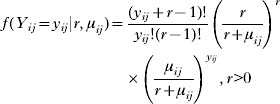
The negative binomial model assumes that the variance of the counts, var(Y ij) is equal to

with k=1/r, known as aggregation parameter. The Poisson distribution arises as r→∞ (or equivalently k→0) and thus var(Y ij)=μij.
ZI models
The ZI count models have mixed specifications that add extra weight to the probability of observing a zero (Lambert, Reference Lambert1992). In particular they are mixture models having two components and mixing probability, π related to the proportion of non-infected individuals who have no chance to be infected. (1−π) corresponds to the probability of observing a positive egg count arising from an adopted count distribution f(y ij) such as Poisson or negative binomial. In the general form, the model can be written as:

where I {0}(y ij) is the one-point distribution, putting all its mass at zero, that is I {0}(y ij)=1 if y ij=0 and zero otherwise. Equivalently the model can be specified by:

The ZIP model has the Poisson density f(y ij)=(1−π)exp(−μij)μijyij/y ij!, y ij>0 and the ZINB model has the negative binomial density function which is given in equation (1). The mean of the ZI model is equal to πI {0}(y ij)+(1−π)μij(1−I {0}(y ij)) and the variance is Var(Y ij)=(1−π)2Var f(Y ij), where Var f(Y ij)=μij for the ZIP model and it is given in equation (2) for the ZINB model.
Bayesian non-stationary overdispersed count model
In the above negative binomial and ZI models we introduce covariates X ij and village-specific spatial random effect φi on the log(μij), that is log(μij)=X ijTβ+φi, where β is the vector of regression coefficients. We assume that the random effects model a continuous spatial process that is φ=(φ1, φ2, …, φN)T~;MVN(0,Σ), has a multivariate normal distribution with variance-covariance matrix Σil=σ2exp(−ρd il), where d il is the shortest straight-line distance between villages i and l, σ2 is the geographic variability known as the sill, and ρ is a smoothing parameter that controls the rate of correlation decay with increasing distance. To take into account non-stationarity, we partitioned the study area in K ecologic sub-regions, i.e. watersheds of the local hydrology (Beck-Wörner et al. Reference Beck-Wörner, Raso, Vounatsou, N'Goran, Rigo, Parlow and Utzinger2007), and assumed a local stationary spatial process  in each sub-region k=1, 2, …, K. We then viewed spatial correlation in our area as a mixture of the different spatial processes and modelled the spatial random effect φi at location i as a weighted average of the sub-region-specific (independent) stationary processes as follows:
 , with weights a ik, which are decreasing functions of the distance between location i and the centroids of the sub-regions k (Banerjee et al. Reference Banerjee, Gelfand, Knight and Sirmans2004). Assuming
 , (Σk)il=σk2exp(−ρkd il), we have
 , where A k=diag{a 1k, a 2k, …, a nk}. The range is defined as the minimum distance at which spatial correlation between locations is below 5% and it can be calculated as
 .
Model fit and implementation
Model fit was carried out in WinBUGS version 1.4 (Imperial College & Medical Research Council, London, UK) and in specialized Bayesian geostatistical codes written in Fortram 95 by the authors. Following a Bayesian model specification, we adopted prior distributions for the model parameters. We choose vague Normal distributions for the β parameters with large variances (i.e. 10 000), gamma prior for r with large variance, inverse gamma priors for σk2 and uniform priors for ρk, k=1, 2, …, K. MCMC simulation was employed to estimate the model parameters (Gelfand and Smith, Reference Gelfand and Smith1990). We ran a single chain sampler with a burn-in of 5000 iterations. Convergence was assessed by inspection of ergodic averages of selected model parameters. Covariates from the multivariate model were used to generate a smooth risk map for S. mansoni infection intensity using Bayesian kriging (Diggle et al. Reference Diggle, Moyeed and Tawn1998).
Model validation
For the model validation a training sample from the current database was used. From the 55 schools, 43 schools were randomly selected and fitted into the models. The remaining 12 schools were used for validation purposes. Validation was done at the individual level to take into account age, sex and socio-economic status as these factors significantly influenced S. mansoni infection intensity (n=731 children). The predictive ability of the models was assessed by calculating for each model credible intervals (the equivalent of confidence interval in Bayesian statistics) with probability coverage varying between 1% and 100% of the posterior predictive distribution of test data. The model with the best predictive ability was the one with the highest percentage of locations within the interval of smallest coverage.
Results
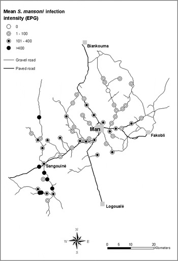
Complete demographic, socio-economic and parasitological data were available for 3818 schoolchildren. The S. mansoni infection prevalence was 38·9% with a mean egg count among infected children of 162 EPG (range: 24 to 6768 EPG). Fig. 1 shows the average S. mansoni infection intensity at the unit of the school; the mean egg excretion ranged from 0 to 875 EPG.
Observed mean S. mansoni infection intensity at the unit of the school in the region of Man, western Côte d'Ivoire.

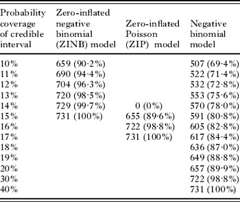
The non-stationary ZINB model showed a better fit to the data than the ZIP model and the negative binomial model. Table 1 summarizes the results from the model validation, according to the percentage of test data with S. mansoni infection intensity falling within credible intervals of probability coverage ranging between 10% and 40%. The ZINB model included 100% of the test data in the narrowest 15% credible interval.
Absolute and cumulative frequency of S. mansoni infection intensity among 731 schoolchildren within the 12 test locations falling within credible intervals of probability coverage ranging between 10% and 40% of the posterior predictive distribution

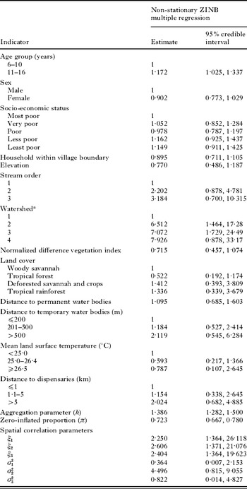
Table 2 displays the results from the best fitting non-stationary ZINB regression model. The covariates that explained significantly the geographical variation of S. mansoni infection intensity were age group and watershed, since the mean coefficient estimates were within the credible intervals. The ZI mixing proportion parameter (π) was 0·723 (95% credible interval=0·667–0·780) suggesting that the proportion of zero counts which was higher than that assumed by the negative binomial distribution was 72·3%. A possible interpretation could be that over half of children who tested negative had no chance to be infected with S. mansoni because they were not exposed. The aggregation parameter k was estimated equal to 1·386 (95% credible interval=1·282–1·500), indicating that there is still over-dispersion even though some of the excessive zeros have been modelled separately. The range parameters ξk, k=1, 2, …, K were similar for the three fixed tiles, indicating that spatial correlation was not significant at distances of approximately 2·6 km and above. In contrast, the geographical variability varied between the tiles from 0·364 to 4·496 indicating non-stationarity.
Posterior summaries (medians and 95% credible intervals) of the parameters of the non-stationary ZINB multiple regression. The estimate of the regression coefficients parameters represent density ratio (DR) of excreted egg counts. The range parameters ξk, k=1,2,3 are given in km

a Arbitrary measure (for further details; see Beck-Wörner et al. Reference Beck-Wörner, Raso, Vounatsou, N'Goran, Rigo, Parlow and Utzinger2007).
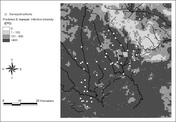
Fig. 2 displays the S. mansoni intensity risk obtained from the non-stationary ZINB regression model. The model predicted low intensities in the north-eastern part of the study area, and high infection intensities in the southern and north-western region. The highest intensities were predicted along the rivers.
Smoothed map of S. mansoni infection intensity based on the Bayesian geostatistical ZINB model.

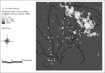
The lowest prediction error of the infection intensity was estimated in the north-eastern part of the study area, where accordingly the infection intensity was predicted to be low (Fig. 3).
Prediction error of S. mansoni infection intensity based on the Bayesian geostatistical ZINB model.

IMPLICATIONS OF OUR FINDINGS AND FUTURE RESEARCH DIRECTIONS
Areas of intensive schistosomiasis transmission are usually associated with a high morbidity, and hence burden of the disease. Although schistosomiasis prevalence maps are useful tools in guiding control interventions (Brooker et al. Reference Brooker, Rowlands, Haller, Savioli and Bundy2000; Raso et al. Reference Raso, Matthys, N'Goran, Tanner, Vounatsou and Utzinger2005; Clements et al. Reference Clements, Lwambo, Blair, Nyandindi, Kaatano, Kinung'hi, Webster, Fenwick and Brooker2006a; Brooker, Reference Brooker2007), maps of transmission intensity provide additional information on the severity of the infection. Such maps allow identification of hot spots with potentially high morbidity and the largest attributable disease fraction, and hence provide insight about where to target ‘preventive chemotherapy’ for morbidity control. Geostatistical models which are based on realistic assumptions about the distributions which generated the intensity data, including the underlying spatial processes, will provide more accurate estimation of the environment-transmission relations, and hence improve the current prediction accuracies (Brooker, Reference Brooker2007).
A general feature of helminth egg output data is that approximately one-fifth of the population are responsible for an estimated 80% of the environmental contamination (Anderson and May, Reference Anderson and May1985). It follows that the egg count data which quantify transmission intensity usually include a large number of zeros or very light infections, which lead to overdispersion. Hence, the variance of such a typical helminth egg distribution is considerably larger than the one assumed by the Poisson distribution. Conventionally the negative binomial distribution has been adopted to take into account overdispersion by an alternative variance-mean specification (Cameron and Trivedi, Reference Cameron and Trivedi1986). However, this approach ignores that a proportion of individuals have no exposure to the disease and therefore neglects the process which generated the additional zeros. ZI models explicitly incorporate this process in the modelling framework. The models we have employed in the current application assume that exposed individuals have a probability to be negative according to the Poisson or negative binomial model which is applied to fit the counts. This may be true due to diagnostic error or possibly genetic factors. We could assess this assumption by applying an alternative class of models, the so-called hurdle, two-part or conditional models (Mullahy, Reference Mullahy1986; Heilbron, Reference Heilbron1994), which assume a zero-truncated standard distribution (Poisson or negative binomial) in the exposed group. Such a model would require further modification to take into account the possibility of false-negatives, which otherwise will be wrongly allocated to the unexposed group.
Another extension of the ZI models discussed here arises when allowing covariates not only on the average count of the exposed group, but also on the mixing proportion, that is the proportion of the non-exposed individuals. An issue related with modelling covariates is that of linearity. Environmental covariates influencing the transmission intensity is less likely to have a linear effect on intensity. The standard approach of categorising the covariates relies on arbitrary cut-off values of those covariates. An alternative modelling approach that could be assessed in mapping infection intensity and other transmission-related outcomes could include the use of spline functions (Eubank, Reference Eubank1988; Dimatteo, Genovese and Kass, Reference Dimatteo, Genovese and Kass2001). Our own experience with spline regression models in malaria mapping (Gosoniu et al. Reference Gosoniu, Vounatsou, Sogoba, Maire and Smith2009) suggests that this is a promising approach, when taking into account non-linearity in disease mapping.
Non-stationarity is an important aspect of geographically-explicit databases, which should be considered, especially when fitting spatial models over large areas. The non-stationary modelling approach we have adopted here relies on a partition of the study region into meaningful ecological sub-regions, such as those governed by water catchment areas (Beck-Wörner et al. Reference Beck-Wörner, Raso, Vounatsou, N'Goran, Rigo, Parlow and Utzinger2007). This approach is more appropriate when modelling schistosomiasis data over large areas covering different ecological zones which define the fixed partitions. An extension of the model will allow different covariate effects in each zone since it is likely to have an interaction effect between the zone and environmental effects on transmission. The model, in addition, smoothes the estimates at the border of the regions, and hence avoids discontinuities, which would otherwise arise (Sogoba et al. Reference Sogoba, Vounatsou, Bagayoko, Doumbia, Dolo, Gosoniu, Traoré, Touré and Smith2007).
Another form of non-stationarity is anisotropy which implies that spatial correlation depends not only on distance between any pair of locations but also on their relative orientation. To our knowledge, anisotropy has not been considered in any of the schistosomiasis transmission mapping exercises carried out thus far. We speculate that the spatial correlation is stronger on directions towards transmission sites rather than in the opposite direction, governed by hydrological factors upon which the intermediate host snails depend (Kitron et al. Reference Kitron, Clennon, Cecere, Gürtler, King and Vazquez-Prokopec2006; Stensgaard et al. Reference Stensgaard, Jørgensen, Kabatereine, Rahbek and Kristensen2006; Clennon et al. Reference Clennon, King, Muchiri and Kitron2007).
Modelling multiple species parasitic infections is receiving increasing interest recently (Raso et al. Reference Raso, Vounatsou, Singer, N'Goran, Tanner and Utzinger2006a; Brooker and Clements, Reference Brooker and Clements2009) as it has been recognised that in tropical and sub-tropical environments multiparasitism is the norm rather than the exception (Raso et al. Reference Raso, Luginbühl, Adjoua, Tian-Bi, Silué, Matthys, Vounatsou, Wang, Dumas, Holmes, Singer, Tanner, N'Goran and Utzinger2004; Utzinger and de Savigny, Reference Utzinger and de Savigny2006; Brooker and Utzinger, Reference Brooker and Utzinger2007; Steinmann et al. Reference Steinmann, Du, Wang, Wang, Jiang, Li, Marti, Zhou and Utzinger2008). Individual exposures or genetic factors are likely to introduce positive or negative correlation in the infection intensities of the different parasites. It is conceivable that control measures can be employed in a more cost-effective manner, once areas of high infection intensities of multiple parasites have been identified and the underlying risk factor(s) determined, so that an integrated control approach can be envisaged. These analyses will require extending the ZIP and the ZINB models to their multivariate analogues, as well as considering multivariate spatial processes (Majumdar and Gelfand, Reference Majumdar and Gelfand2007) to model spatial correlation of coinfection intensity data.
ACKNOWLEDGEMENTS
We thank Dr. J. Russell Stothard for inviting us to prepare this article for a special issue of Parasitology. With regard to the motivating example, we thank the education officers, the school directors and teachers, the participating schoolchildren, and the field and laboratory team for their commitment. PV (project no. 3252B0-102136), GR (project no. PBBSB-109011) and JU (project no. PPOOB-102883, PPOOB-119129) are financially supported by the Swiss National Science Foundation. GR also received funds from Novartis Foundation, the Roche Research Foundation through a fellowship and the University of Queensland for a postdoctoral research fellowship.