1 Introduction
Many fish and marine mammals swim by using a combination of an active swimming phase and a passive coasting phase known as burst-and-coast or burst-and-glide swimming (Videler Reference Videler1981; Videler & Weihs Reference Videler and Weihs1982; Müller, Stamhuis & Videler Reference Müller, Stamhuis and Videler2000; Kramer & McLaughlin Reference Kramer and McLaughlin2001; Williams Reference Williams2001; Wu, Yang & Zeng Reference Wu, Yang and Zeng2007; Gleiss et al. Reference Gleiss, Jorgensen, Liebsch, Sala, Norman, Hays, Quintana, Grundy, Campagna and Trites2011; Takagi, Tamura & Weihs Reference Takagi, Tamura and Weihs2013). This intermittent swimming gait adopted by fish, has been predicted by dynamical models to yield an energy saving to swim a given distance of over 50 % (Weihs Reference Weihs1974, Reference Weihs1980). These predictions are based on the Bone–Lighthill boundary layer thinning hypothesis, which proposes that there is an increase in skin friction drag on a fish body when it undulates (Lighthill Reference Lighthill1971). Under these conditions, a fish may then reduce its overall skin friction drag by interspersing an undulation phase with a coasting phase. The skin friction increase is caused by the thinning of the boundary layer from the body-normal velocity component that is present during undulation. In fact, Lighthill originally estimated that the skin friction drag on a swimming body can be up to a factor of 5 times larger than a gliding body (Lighthill Reference Lighthill1971). Others estimated that the factor could be in a range of 4–10 (Webb Reference Webb1975; Videler Reference Videler1981; Wu et al. Reference Wu, Yang and Zeng2007). More recently, detailed analysis confirms the boundary layer thinning hypothesis, but estimates the skin friction drag increase to be much more modest than originally proposed and in the range of a 20–70 % drag increase (Ehrenstein & Eloy Reference Ehrenstein and Eloy2013; Ehrenstein, Marquillie & Eloy Reference Ehrenstein, Marquillie and Eloy2014).
Given this range of skin friction increase, the total drag of a low Reynolds number swimmer of
 $O(10^{3})$
and a high Reynolds number swimmer of
 $O(10^{6})$
will only increase by 34 % and 46 %, respectively, when typical ratios of skin friction and form drag are considered. By using these scaling estimates in Weihs’ dynamical model (Weihs Reference Weihs1974) energy savings of 14 % and 19 % are predicted for low and high Reynolds number swimmers, respectively. Furthermore, experiments conducted on a swimming trout reveal that although the skin friction increases on one side of the fish, the opposite side of the fish has a skin friction decrease cancelling out the net skin friction rise when averaged over the full cycle of motion (Yanase & Saarenrinne Reference Yanase and Saarenrinne2015, Reference Yanase and Saarenrinne2016). It is then clear that the viscous mechanism proposed by Bone and Lighthill (Reference Lighthill1971) is not sufficient to create a 50 % saving in energy by itself. Yet, a 45 % energy saving was indirectly estimated from digital particle image velocimetry (DPIV) experiments that measured the thrust impulse imparted to the wake of koi carps (Wu et al.
Reference Wu, Yang and Zeng2007). Also, a 56 % energy saving for an intermittent fish-like swimmer was directly calculated by using a two-dimensional Navier–Stokes solver (Chung Reference Chung2009).
Motivated by these observations, we hypothesize that there is an inviscid mechanism that can account for the majority of the energetic benefit seen in intermittent swimming for parameters typical of biology. To examine this hypothesis, we show that by using inviscid computations there is an energy saving for intermittent swimming as compared to continuous swimming at the same swimming speed. Then we consider three questions: How do the forces and energetics of intermittent swimming scale with the swimming parameters, what is the nature of the inviscid mechanism that leads to the observed energy savings and what are the limitations of the benefit?
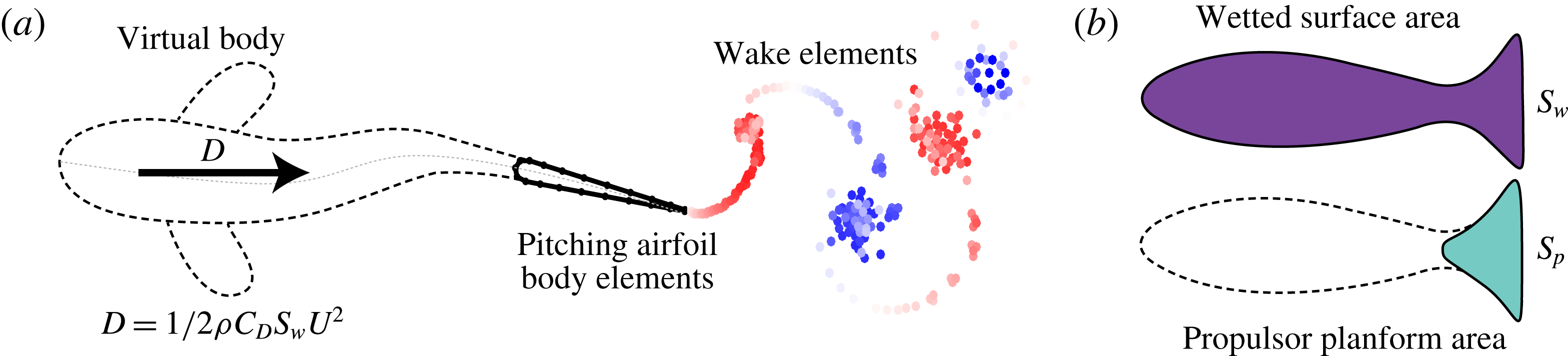
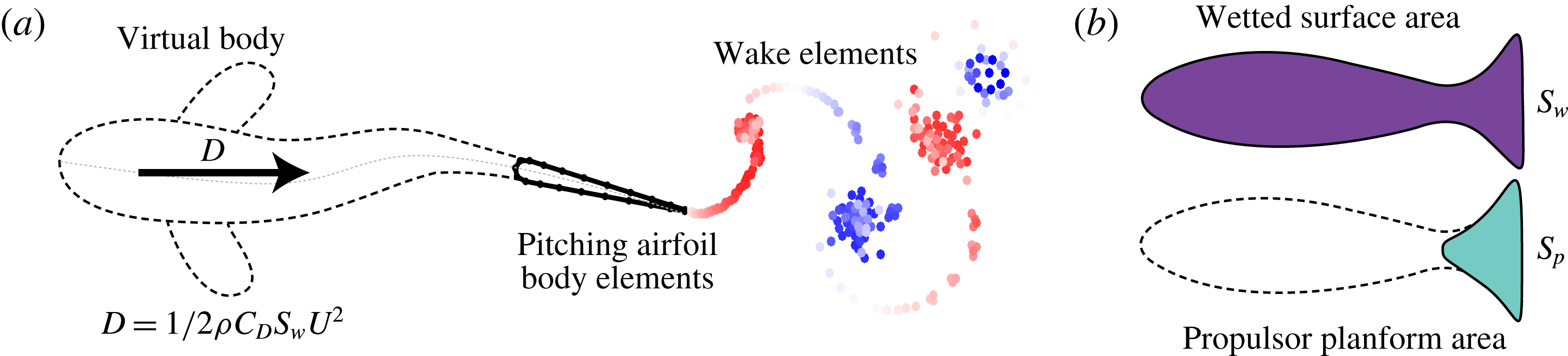
(a) Schematic of the idealized self-propelled swimmer. Dashed line represents the virtual body. There is a drag force,
 $D$
, acting on the hydrofoil that represents the effect of the virtual body. The wake element endpoints are coloured red and blue for counter clockwise and clockwise circulation, respectively. (b) Schematic representation of the wetted surface area,
 $S_{w}$
, (purple shaded area) and the propulsor area,
 $S_{p}$
, (teal shaded area) for a generic swimmer.
2 Approach and numerical methods
2.1 Problem formulation and input parameters
A computational study is performed to compare the performance and flow fields of idealized continuous and intermittent swimmers. A self-propelled swimmer is used to model the problem that is a combination of a virtual body and a two-dimensional hydrofoil pitching about its leading edge (figure 1
a). The virtual body is not present in the computational domain, however, its presence is modelled as a drag force,
 $D$
, that acts to resist the motion of the swimmer. The magnitude of the drag force is determined from a drag law based on high Reynolds number swimming conditions (Munson, Young & Okiishi Reference Munson, Young and Okiishi1990),
 $$\begin{eqnarray}\displaystyle D=1/2\,\unicode[STIX]{x1D70C}C_{D}S_{w}U^{2}, & & \displaystyle\end{eqnarray}$$
where
 $\unicode[STIX]{x1D70C}$
is the density of the fluid,
 $C_{D}$
is the coefficient of drag of the virtual body,
 $S_{w}$
is the combined wetted surface area of the virtual body and the propulsor (figure 1
b) and
 $U$
is the speed of the swimmer. The planform area of the hydrofoil,
 $S_{p}$
, is defined as the chord length,
 $c$
, multiplied by a unit span length. The chord length is fixed to
 $c=0.07$
m, which is typical of species that use intermittent swimming gaits (Beamish Reference Beamish1966; Videler Reference Videler1981). An area ratio can then be formed as the ratio of the wetted surface area to the propulsor planform area,
 $$\begin{eqnarray}\displaystyle S_{wp}\equiv \frac{S_{w}}{S_{p}}. & & \displaystyle\end{eqnarray}$$
The area ratio, used to calculate
 $S_{w}$
in the drag law, is selected to be
 $S_{wp}=8$
, which is also typical for intermittently swimming species (Beamish Reference Beamish1966; Videler Reference Videler1981; Videler & Wardle Reference Videler and Wardle1991; Webber et al.
Reference Webber, Boutilier, Kerr and Smale2001). In addition, the pitching hydrofoil has a teardrop cross-sectional shape (Marais et al.
Reference Marais, Thiria, Wesfreid and Godoy-Diana2012) with a thickness-to-chord ratio of
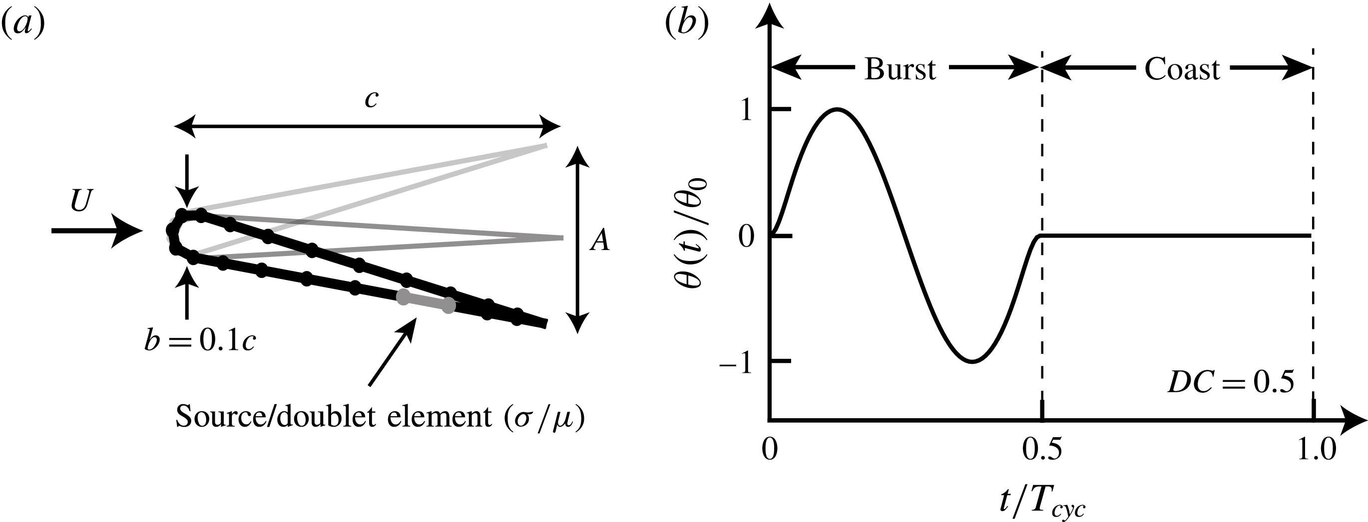
 $b/c=0.1$
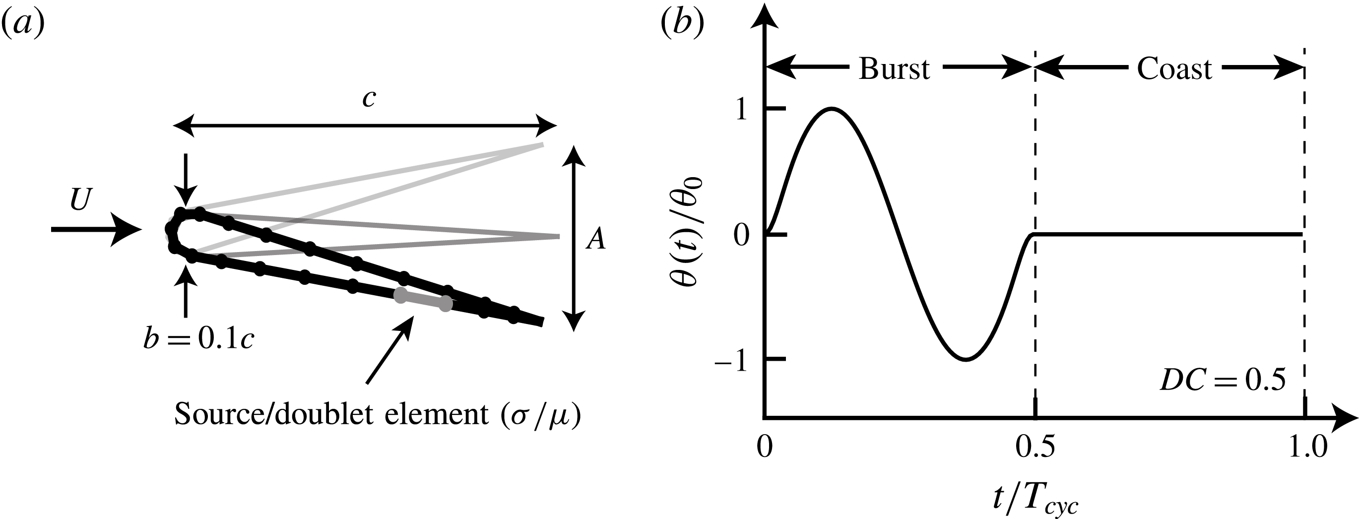
(see figure 2
a).
Previous analytical and computational models of intermittent swimming assume a higher
 $C_{D}$
during a bursting phase than a gliding phase by referring to the Bone–Lighthill boundary layer thinning hypothesis (Weihs Reference Weihs1974; Müller et al.
Reference Müller, Stamhuis and Videler2000; Wu et al.
Reference Wu, Yang and Zeng2007; Chung Reference Chung2009). However, in this study we set
 $C_{D}$
to be a constant value for both the bursting and gliding phases of intermittent swimming. This allows us to probe the hypothesis that the energy saving observed in intermittent swimming is not wholly due to the boundary layer thinning hypothesis. In other words, when
 $C_{D}$
is fixed regardless of whether a swimmer is oscillating its fin or gliding, then any observed energy saving comes purely from potential flow mechanisms and is not associated with a skin friction rise due to the oscillating fin and/or body. In this study, three different constant drag coefficients,
 $C_{D}=0.005,0.01$
and 0.05, are used to represent the range of average drag coefficients observed in biology (Videler Reference Videler1981; Videler & Weihs Reference Videler and Weihs1982; Webb, Kostecki & Stevens Reference Webb, Kostecki and Stevens1984; Anderson, McGillis & Grosenbaugh Reference Anderson, McGillis and Grosenbaugh2001; Wu et al.
Reference Wu, Yang and Zeng2007; Ehrenstein & Eloy Reference Ehrenstein and Eloy2013; Ehrenstein et al.
Reference Ehrenstein, Marquillie and Eloy2014).
(a) Geometric and numerical parameters for the teardrop hydrofoil. (b) Normalized pitching angle as a function of normalized time for an intermittent swimmer with
 $DC=0.5$
.
The drag coefficient and the area ratio can be grouped together into a combination parameter known as the Lighthill number (Eloy Reference Eloy2013),
 $$\begin{eqnarray}\displaystyle Li=C_{D}\,S_{wp}. & & \displaystyle\end{eqnarray}$$
The Lighthill number characterizes how the body and propulsor geometry affect the balance of thrust and drag forces on a swimmer. For example, for a fixed swimming speed and propulsor area, a high Lighthill number means that the body of the swimmer will have high drag and vice versa. One physical interpretation of the Lighthill number is that it indicates how streamlined a swimmer is with a high
 $Li$
representing a poorly streamlined swimmer. The streamlining of a swimmer will consequently affect the fin loading on the propulsor, analogous to wing loading in birds, leading to an alternative interpretation of
 $Li$
. By using the definition of drag and the fact that the thrust and drag must balance in self-propelled swimming, the Lighthill number may be alternatively defined as the thrust coefficient based on the dynamic pressure, that is,
 $Li=(T/S_{p})/(1/2\,\unicode[STIX]{x1D70C}U^{2})=C_{T}^{dyn}$
. This non-dimensional fin loading is high for high
 $Li$
and vice versa. In the present study, the Lighthill numbers examined are
 $Li=0.04,\,0.08$
and 0.4, which fall in a range typical of biology (Eloy Reference Eloy2013).
The virtual body also must be given a mass,
 $m$
, which can be non-dimensionalized with the added mass of the hydrofoil propulsor, that is,
 $$\begin{eqnarray}\displaystyle m^{\ast }\equiv \frac{m}{\unicode[STIX]{x1D70C}S_{p}c}. & & \displaystyle\end{eqnarray}$$
The non-dimensional mass,
 $m^{\ast }$
, affects not only the acceleration of a swimmer due to any net time-averaged forces over a period, but it also affects the magnitude of the surging oscillations that occur within a period due to the unsteady forcing of the pitching hydrofoil. By using the mass of a typical intermittent swimmer and the dimensions of the pitching hydrofoil, the non-dimensional mass is set to
 $m^{\ast }=3.86$
throughout this study. Even though this mass ratio is based on the biology, previous self-propelled numerical solutions show that the time-averaged forces and energetics are effectively independent of the amplitude of surging oscillations for
 $m^{\ast }>1$
(Moored & Quinn Reference Moored and Quinn2017) even though the instantaneous forces can be affected (Wen & Lauder Reference Wen and Lauder2013).
The kinematic motion is parameterized with a pitching frequency,
 $f$
, and a peak-to-peak trailing-edge amplitude,
 $A$
, reported as a non-dimensional amplitude-to-chord ratio,
 $A^{\ast }=A/c$
, and a duty cycle,
 $DC$
. The amplitude-to-chord ratio is related to the maximum pitch angle, that is,
 $\unicode[STIX]{x1D703}_{0}=\sin ^{-1}(A^{\ast }/2)$
. The degree of intermittency of swimming is captured in the duty cycle, which is,
 $$\begin{eqnarray}\displaystyle DC=\frac{\text{burst period}}{\text{total cycle period}}=\frac{T_{burst}}{T_{cycle}}. & & \displaystyle\end{eqnarray}$$
Figure 2(b) shows a characteristic pitching motion with the burst, coast and total cycle periods defined. The intermittent motion is a combination of a sinusoidal pitching motion for the burst period and it is followed by a fixed pitch angle of
 $\unicode[STIX]{x1D703}=0$
for the duration of the coast period. The total cycle period is simply the addition of the burst and coast periods. The combined burst and coast pitching motions about the leading edge of the hydrofoil is then defined as,
 $$\begin{eqnarray}\displaystyle \unicode[STIX]{x1D703}(t)=\left\{\begin{array}{@{}ll@{}}y_{s}(t)[\unicode[STIX]{x1D703}_{0}\sin (2\unicode[STIX]{x03C0}ft)],\quad & 0\leqslant t\leqslant T_{burst},\\ 0,\quad & T_{burst}\leqslant t\leqslant T_{cycle},\end{array}\right. & & \displaystyle\end{eqnarray}$$
where
 $$\begin{eqnarray}\displaystyle y_{s}(t)=\left\{\begin{array}{@{}ll@{}}-\tanh (m\,t)\,\tanh [m\,(t-1)],\quad & DC<1,\\ 1,\quad & DC=1.\end{array}\right. & & \displaystyle\end{eqnarray}$$
Equation (2.6) defines a reference signal where
 $0\leqslant t\leqslant T_{cycle}$
. The signal used in the simulations has
 $N_{cyc}$
repetitions of this reference signal. Here,
 $T_{burst}=1/f$
and
 $T_{cycle}=T_{burst}/DC$
.
In order to obtain discretization independent solutions as the time step size is reduced, the discontinuous angular rates and accelerations at the junction of the burst phase and coast phase must be smoothed. To do this, a hyperbolic tangent envelope function,
 $y_{s}(t)$
, is multiplied with the sinusoidal burst signal and is defined in (2.7). This function modifies the slope of the sine wave at
 $t/T_{burst}=0$
and
 $t/T_{burst}=1$
to ensure a desingularized smooth junction with the coast phase where
 $m$
controls the radius of curvature of the junction. In the current study,
 $m=9$
is used. Additionally, if
 $DC=1$
, then the signal (2.6) reverts to a continuous sinusoidal signal. In the current study the duty cycle ranges from
 $DC=0.2$
to
 $DC=1$
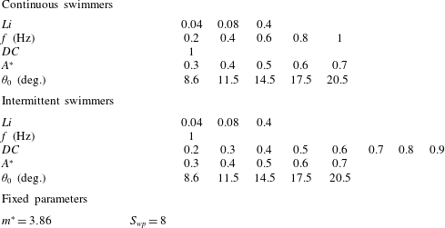
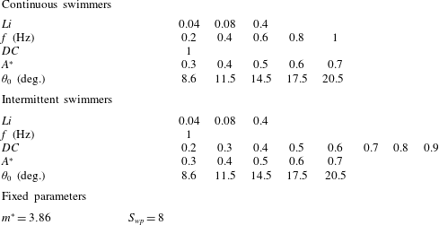
in 0.1 increments. A summary of the input parameters used in the current study are in table 1.
2.2 Numerical methods
To model a high Reynolds number fluid flow, the field around the hydrofoils is assumed inviscid, irrotational (except on the boundary elements) and incompressible. For an incompressible and irrotational fluid the continuity equation reduces to Laplace’s equation,
 $\unicode[STIX]{x1D6FB}^{2}\unicode[STIX]{x1D719}^{\ast }=0$
, where
 $\unicode[STIX]{x1D719}^{\ast }$
is the perturbation potential in an inertial frame fixed to the undisturbed fluid. In addition, the no-flux boundary condition must be satisfied on the body’s surface,
 ${\mathcal{S}}_{b}$
that is,
 $$\begin{eqnarray}\displaystyle \unicode[STIX]{x1D735}\unicode[STIX]{x1D719}^{\ast }\boldsymbol{\cdot }\boldsymbol{n}=0\quad \text{on}~{\mathcal{S}}_{b}, & & \displaystyle\end{eqnarray}$$
where
 $\boldsymbol{n}$
is a vector normal to the body’s surface, and the velocity is
 $\boldsymbol{u}=\unicode[STIX]{x1D735}\unicode[STIX]{x1D719}^{\ast }$
. Additionally, the velocity disturbances created by the motion should satisfy the far-field boundary condition and decay far from the body,
 $$\begin{eqnarray}\displaystyle \lim _{r\rightarrow \infty }(\unicode[STIX]{x1D735}\unicode[STIX]{x1D719}^{\ast })=0, & & \displaystyle\end{eqnarray}$$
where
 $\boldsymbol{r}=x\,\hat{\boldsymbol{x}}+z\,\hat{\boldsymbol{z}}$
measured from a body-fixed frame.
Simulation parameters used in the present study.
Following Katz & Plotkin (Reference Katz and Plotkin2001) and Quinn et al. (Reference Quinn, Moored, Dewey and Smits2014), the general solution for the perturbation potential, also known as the boundary integral equation, is explicitly stated as a combination of a distribution of sources of strength
 $\unicode[STIX]{x1D70E}$
and doublets of strength
 $\unicode[STIX]{x1D707}$
on the body surface
 ${\mathcal{S}}_{b}$
and a distribution of doublets of strength
 $\unicode[STIX]{x1D707}_{w}$
on the wake surface
 ${\mathcal{S}}_{w}$
,
 $$\begin{eqnarray}\displaystyle ~\unicode[STIX]{x1D719}_{i}^{\ast }(\boldsymbol{r})=\unicode[STIX]{x0222F}_{{\mathcal{S}}_{b}}[\unicode[STIX]{x1D70E}(\boldsymbol{r}_{\mathbf{0}})\,G(\boldsymbol{r};\boldsymbol{r}_{\mathbf{0}})-\unicode[STIX]{x1D707}(\boldsymbol{r}_{\mathbf{0}})\,\hat{\boldsymbol{n}}\boldsymbol{\cdot }\unicode[STIX]{x1D735}G(\boldsymbol{r};\boldsymbol{r}_{\mathbf{0}})]\,\text{d}{\mathcal{S}}_{0}-\unicode[STIX]{x0222F}_{{\mathcal{S}}_{w}}\unicode[STIX]{x1D707}_{w}(\boldsymbol{r}_{\mathbf{0}})\,\hat{\boldsymbol{n}}\boldsymbol{\cdot }\unicode[STIX]{x1D735}G(\boldsymbol{r};\boldsymbol{r}_{\mathbf{0}})\,\text{d}{\mathcal{S}}_{0},\hspace{-6.99997pt} & & \displaystyle \nonumber\\ \displaystyle & & \displaystyle\end{eqnarray}$$
where,
 $$\begin{eqnarray}\displaystyle & \displaystyle \unicode[STIX]{x1D70E}=\hat{\boldsymbol{n}}\boldsymbol{\cdot }\unicode[STIX]{x1D735}(\unicode[STIX]{x1D719}^{\ast }-\unicode[STIX]{x1D719}_{i}^{\ast }), & \displaystyle\end{eqnarray}$$
 $$\begin{eqnarray}\displaystyle & \displaystyle -\unicode[STIX]{x1D707}=\unicode[STIX]{x1D719}^{\ast }-\unicode[STIX]{x1D719}_{i}^{\ast }, & \displaystyle\end{eqnarray}$$
 $$\begin{eqnarray}\displaystyle & \displaystyle -\unicode[STIX]{x1D707}_{w}=\unicode[STIX]{x1D719}_{+}^{\ast }-\unicode[STIX]{x1D719}_{-}^{\ast }. & \displaystyle\end{eqnarray}$$
Here
 $\unicode[STIX]{x1D719}_{i}^{\ast }$
is the internal potential,
 $\boldsymbol{r}_{\mathbf{0}}$
is the location of a source or doublet,
 $\boldsymbol{r}$
is the target point and Green’s function for the two-dimensional Laplace equation is
 $G(\boldsymbol{r};\,\boldsymbol{r}_{0})=(1/2\unicode[STIX]{x03C0})\ln |\boldsymbol{r}-\boldsymbol{r}_{\mathbf{0}}|$
. Conveniently, doublets and sources both implicitly satisfy the far-field boundary condition (2.9). The problem is then reduced to determining the source distribution,
 $\unicode[STIX]{x1D70E}$
, and the doublet distribution,
 $\unicode[STIX]{x1D707}$
, over the surfaces such that the no-flux boundary condition (2.8) is satisfied. Here a Dirichlet formulation is used to enforce the boundary condition by fixing the potential within the body surface to be equal to zero, that is,
 $\unicode[STIX]{x1D719}_{i}^{\ast }=0$
. This leads to the potential field at the surface of the body equated to the local doublet strength as
 $-\unicode[STIX]{x1D707}=\unicode[STIX]{x1D719}_{b}^{\ast }$
and the local velocity normal to the body surface equated to the source strength as
 $\unicode[STIX]{x1D70E}=\hat{\boldsymbol{n}}\boldsymbol{\cdot }\unicode[STIX]{x1D735}\unicode[STIX]{x1D719}_{b}^{\ast }=\hat{\boldsymbol{n}}\boldsymbol{\cdot }(\boldsymbol{u}_{rel}+\boldsymbol{U})$
. The velocity of the centre of each source element is
 $\boldsymbol{u}_{rel}$
, which is relative to a body-fixed frame of reference located at the leading edge of the hydrofoil and
 $\boldsymbol{U}$
is the velocity of the body-fixed frame with respect to the undisturbed fluid.
To solve the problem numerically, surface
 ${\mathcal{S}}_{b}$
is discretized into
 $N$
source and doublet boundary elements and surface
 ${\mathcal{S}}_{w}$
is discretized into
 $N_{w}$
doublet boundary elements. Each line element is formed of a constant strength distribution of point sources or doublets. In addition, the no-flux Dirichlet boundary condition (equation (2.10) with
 $\unicode[STIX]{x1D719}_{i}^{\ast }=0$
) is enforced at
 $N$
discrete collocation points. These points are located at the centre of the elements moved inside the hydrofoil along the surface normal vector by 15 % of the body half-thickness. Also, an explicit Kutta condition is applied by introducing a wake panel at the trailing edge with a strength
 $\unicode[STIX]{x1D707}_{w,TE}=\unicode[STIX]{x1D707}_{t,TE}-\unicode[STIX]{x1D707}_{b,TE}$
where
 $\unicode[STIX]{x1D707}_{t,TE}$
and
 $\unicode[STIX]{x1D707}_{b,TE}$
are the strengths of the top and bottom body elements at the trailing edge, respectively. The trailing-edge wake element is oriented along a line that bisects the upper and lower body surfaces at the trailing edge. The length of the element is set to
 $0.4\,U\unicode[STIX]{x0394}t$
where
 $\unicode[STIX]{x0394}t$
is the time step for the computations.
To satisfy the Kelvin circulation theorem a wake shedding procedure must be applied. At every time step, the first wake panel is ‘shed’ by advecting the element downstream by a distance of
 $U\unicode[STIX]{x0394}t$
while its strength remains fixed for all time at
 $\unicode[STIX]{x1D707}_{w,TE}$
from the previous time step. Subsequently, a new trailing-edge wake element is formed and the shed wake panel is further advected with the local induced velocity field from the other wake and body elements. During this rollup process, the endpoints of the doublet elements, which are mathematically equivalent to point vortices, must be desingularized for the numerical stability of the solution. Following Krasny (Reference Krasny1986) the induced velocity on a wake element from other doublet elements is then calculated with a desingularized Biot–Savart law,
 $$\begin{eqnarray}\displaystyle \boldsymbol{u}(\boldsymbol{r})=\frac{\unicode[STIX]{x1D6E4}}{2\unicode[STIX]{x03C0}}\frac{\hat{\boldsymbol{y}}\times (\boldsymbol{r}-\boldsymbol{r}_{\boldsymbol{i}})}{|\boldsymbol{r}-\boldsymbol{r}_{\boldsymbol{i}}|^{2}+\unicode[STIX]{x1D6FF}^{2}} & & \displaystyle\end{eqnarray}$$
and
 $$\begin{eqnarray}\displaystyle \boldsymbol{r}-\boldsymbol{r}_{\boldsymbol{i}}=(x-x_{i})\,\hat{\boldsymbol{x}}+(z-z_{i})\,\hat{\boldsymbol{z}}. & & \displaystyle\end{eqnarray}$$
Here
 $x_{i}$
and
 $z_{i}$
are the positions of the
 $i$
th endpoint of the doublet elements. The desingularized point vortex circulation is related to its doublet element strength as
 $\unicode[STIX]{x1D6E4}=-\unicode[STIX]{x1D707}$
. As the desingularization parameter,
 $\unicode[STIX]{x1D6FF}$
, approaches zero the classical Biot–Savart law is recovered. In the current study,
 $\unicode[STIX]{x1D6FF}/c=6\times 10^{-2}$
is selected for the desingularization.
A matrix form of the boundary integral equation (2.10) is constructed with
 $\unicode[STIX]{x1D719}_{i}^{\ast }=0$
, the explicit Kutta condition applied and the wake element representation described above governing the development of the free shear layer. The linear equations are solved to determine the unknown body doublet element strengths and subsequently the perturbation potential field
 $\unicode[STIX]{x1D719}^{\ast }(\boldsymbol{r})$
and the velocity field
 $\boldsymbol{u}(\boldsymbol{r})$
. Then the perturbation velocity on the surface of the body is found by a local differentiation of the perturbation potential,
 $$\begin{eqnarray}\displaystyle \boldsymbol{u}_{\boldsymbol{b}}=\unicode[STIX]{x1D735}\unicode[STIX]{x1D719}_{b}^{\ast }=\frac{\unicode[STIX]{x2202}\unicode[STIX]{x1D719}^{\ast }}{\unicode[STIX]{x2202}s}\,\hat{\boldsymbol{s}}+\frac{\unicode[STIX]{x2202}\unicode[STIX]{x1D719}^{\ast }}{\unicode[STIX]{x2202}n}\,\hat{\boldsymbol{n}}=-\frac{\unicode[STIX]{x2202}\unicode[STIX]{x1D707}}{\unicode[STIX]{x2202}s}\,\hat{\boldsymbol{s}}+\unicode[STIX]{x1D70E}\,\hat{\boldsymbol{n}}, & & \displaystyle\end{eqnarray}$$
where
 $\hat{\boldsymbol{s}}$
is the tangential vector along the surface of the body. In addition, the pressure field acting on the body is calculated using the unsteady Bernoulli equation,
 $$\begin{eqnarray}\displaystyle P_{b}(x,z,t)=\unicode[STIX]{x1D70C}\left.\frac{\unicode[STIX]{x2202}\unicode[STIX]{x1D707}}{\unicode[STIX]{x2202}t}\right|_{body}+\unicode[STIX]{x1D70C}(\boldsymbol{u}_{rel}+\boldsymbol{U})\boldsymbol{\cdot }\boldsymbol{u}_{\boldsymbol{b}}-\unicode[STIX]{x1D70C}\frac{\boldsymbol{u}_{\boldsymbol{b}}^{2}}{2}. & & \displaystyle\end{eqnarray}$$
Finally, the forces acting on the pitching hydrofoil are calculated from a combination of the pressure forces acting on the body and the drag law (2.1),
 $$\begin{eqnarray}\boldsymbol{F}(t)=\int _{{\mathcal{S}}_{b}}-P_{b}\,\hat{\boldsymbol{n}}\,\text{d}{\mathcal{S}}_{b}+D\,\hat{\boldsymbol{x}}.\end{eqnarray}$$
To examine intermittent motions the computations are required to model self-propelled swimming conditions. Consequently, a simple single degree of freedom equation of motion, which only allows the streamwise translation of the hydrofoil, is loosely coupled to the boundary element fluid solver. Following Borazjani et al. (Reference Borazjani and Sotiropoulos2009), the velocity of the swimmer at the
 $(n+1)$
th time step is calculated through forward differencing and the position is calculated by using the trapezoidal rule,
 $$\begin{eqnarray}\displaystyle & \displaystyle U^{n+1}=U^{n}+\frac{F_{x,net}^{n}}{m}\unicode[STIX]{x0394}t, & \displaystyle\end{eqnarray}$$
 $$\begin{eqnarray}\displaystyle & \displaystyle x_{LE}^{n+1}=x_{LE}^{n}+{\textstyle \frac{1}{2}}(U^{n+1}+U^{n})\unicode[STIX]{x0394}t, & \displaystyle\end{eqnarray}$$
where
 $F_{x,net}^{n}$
is the net force acting on the hydrofoil in the streamwise direction at the
 $n$
th time step,
 $x_{LE}$
is the leading-edge position of the hydrofoil. The two-dimensional formulation in the current study has been validated extensively against continuous swimming theoretical solutions and experiments (Quinn et al.
Reference Quinn, Moored, Dewey and Smits2014). There is also a three-dimensional counterpart that has been extensively validated and used to examine bio-inspired (Moored Reference Moored2017) and biological self-propelled swimming (Fish et al.
Reference Fish, Schreiber, Moored, Liu, Dong and Bart-Smith2016).
2.3 Output parameters and performance metrics
There are several output parameters used throughout this study. For many of them, we examine their mean values time averaged over an oscillation cycle, which are denoted with an overbar such as
 $\overline{(\boldsymbol{\cdot })}$
. Mean quantities are only taken after a swimmer has reached the steady state of its cycle-averaged swimming speed. When this occurs, the steady-state cycle-averaged swimming speed will be described as the mean swimming speed and denoted as
 $\overline{U}$
. The computations are considered to be at a steady-state condition when there is negligible mean net thrust acting on the swimmer, defined as,
 $$\begin{eqnarray}\displaystyle C_{T,net}=\frac{\overline{T}-\overline{D}}{\unicode[STIX]{x1D70C}S_{p}\overline{U}^{2}}<10^{-4}, & & \displaystyle\end{eqnarray}$$
where
 $\overline{T}$
is the mean thrust force calculated as the streamwise force from the pressure integration term in (2.18) alone. The Strouhal number and the reduced frequency are typical non-dimensional frequencies used in bio-propulsion studies and are defined as,
 $$\begin{eqnarray}\displaystyle St=\frac{fA}{\overline{U}},\quad k=\frac{fc}{\overline{U}}. & & \displaystyle\end{eqnarray}$$
The Strouhal number represents the ratio of the cross-stream spacing to the streamwise spacing of the vortices in the wake of a swimmer. The reduced frequency is a ratio of the time that is takes a fluid particle to traverse the chord of the hydrofoil compared to the period of motion and is a measure of the unsteadiness of the flow. Since in self-propelled swimming the mean speed is unknown a priori both the Strouhal number and the reduced frequency are also unknown a priori. The time-averaged thrust and power coefficients depend upon the Strouhal number and the reduced frequency and are,
 $$\begin{eqnarray}\displaystyle C_{T}\equiv \frac{\overline{T}}{\unicode[STIX]{x1D70C}S_{p}\hspace{1.0pt}f^{2}A^{2}},\quad C_{P}\equiv \frac{\overline{P}}{\unicode[STIX]{x1D70C}S_{p}\hspace{1.0pt}f^{2}A^{2}\overline{U}}. & & \displaystyle\end{eqnarray}$$
These coefficients are non-dimensionalized with the added-mass forces and added-mass power from linear theory (Garrick Reference Garrick1936). Additionally, the mean power input to the fluid is calculated as the negative inner product of the force vector and velocity vector of each boundary element. The ratio of these coefficients leads to the propulsive efficiency,
 $\unicode[STIX]{x1D702}$
, which is linked to the cost of transport,
 $CoT$
,
 $$\begin{eqnarray}\displaystyle \unicode[STIX]{x1D702}=\frac{\overline{TU}}{\overline{P}},\quad CoT=\frac{\overline{P}}{m\overline{U}}. & & \displaystyle\end{eqnarray}$$
The propulsive efficiency,
 $\unicode[STIX]{x1D702}$
, is defined as the ratio of useful mean power output to the mean power input to the fluid. In self-propelled swimming we define this quantity in the potential flow sense (Lighthill Reference Lighthill1971), that is, the mean thrust force is calculated as the integration of the pressure forces alone. In this sense the propulsive efficiency is not ill defined for self-propelled swimming as is the case when the net thrust force is used. The cost of transport is a measure of the amount of energy it takes to swim a unit distance reported on a per unit mass basis. It is widely used throughout the biological literature (Videler & Wardle Reference Videler and Wardle1991) and is a useful engineering metric since its inverse is the proportionality constant between the range of a vehicle,
 ${\mathcal{R}}$
, and its energy density (
 ${\mathcal{E}}\equiv \text{energy per unit mass}=E/m$
), that is,
 ${\mathcal{R}}=(1/CoT){\mathcal{E}}$
.
To compare the energetic performance of an intermittent swimmer with a continuous swimmer at the same mean speed the normalized cost of transport and efficiency are introduced,
 $$\begin{eqnarray}\displaystyle \hat{CoT}\equiv \left.\frac{CoT_{int}}{CoT_{cont}}\right|_{\overline{U}},\quad \hat{\unicode[STIX]{x1D702}}\equiv \left.\frac{\unicode[STIX]{x1D702}_{int}}{\unicode[STIX]{x1D702}_{cont}}\right|_{\overline{U}}. & & \displaystyle\end{eqnarray}$$
Here the cost of transport of an intermittent and continuous swimmer are
 $CoT_{int}$
and
 $CoT_{cont}$
, respectively, and the efficiency of an intermittent and continuous swimmer are
 $\unicode[STIX]{x1D702}_{int}$
and
 $\unicode[STIX]{x1D702}_{cont}$
, respectively.
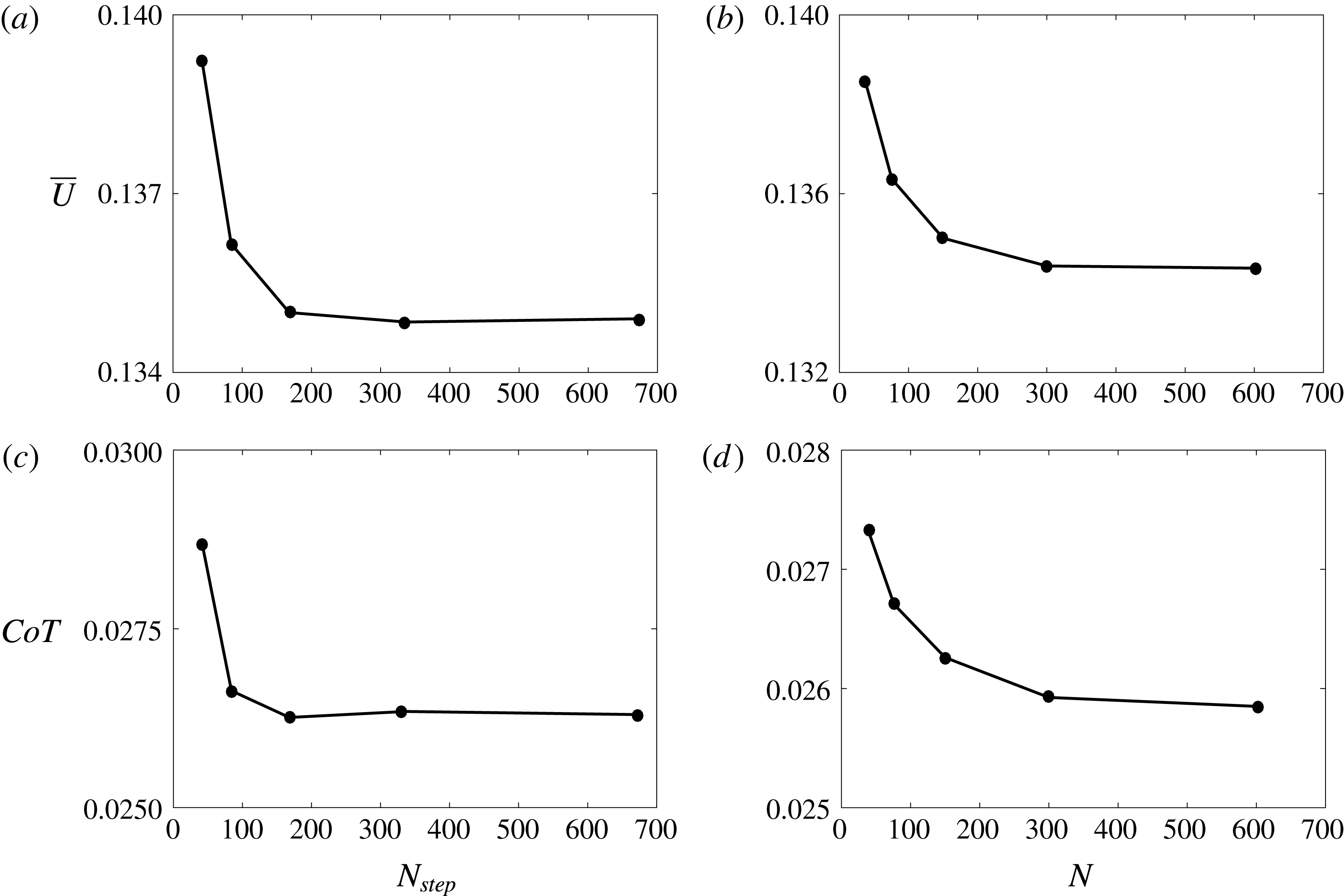
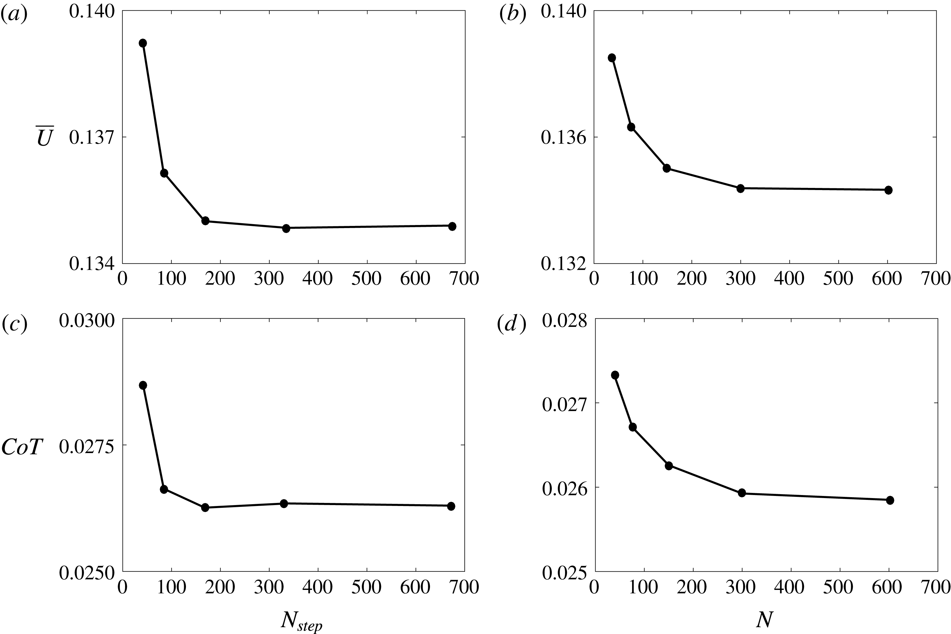
Mean swimming speed as a function of the (a) number of time steps during the bursting period and (b) number of body elements. Cost of transport as a function of the (c) number of time steps during the bursting period and (d) number of body elements. For these discretization independence simulations the parameters used are
 $Li=0.08,A^{\ast }=0.5,DC=0.5$
and
 $f=1$
Hz.
2.4 Discretization independence
Figure 3 shows the mean swimming speed and cost of transport as a function of the number of body elements and the number of time steps during the bursting period used in the simulations. The parameters used are
 $Li=0.08,A^{\ast }=0.5,DC=0.5$
and
 $f=1$
Hz. It is evident that the mean speed and cost of transport are converging to discretization independent solutions as the number of body elements and time steps is increased. Both performance metrics change by less than 2 % when
 $N=150$
is doubled or
 $N_{step}=150$
is doubled. Therefore throughout this study these values for the number of body elements and number of time steps during the bursting period will be used.
3 Results
3.1 Performance
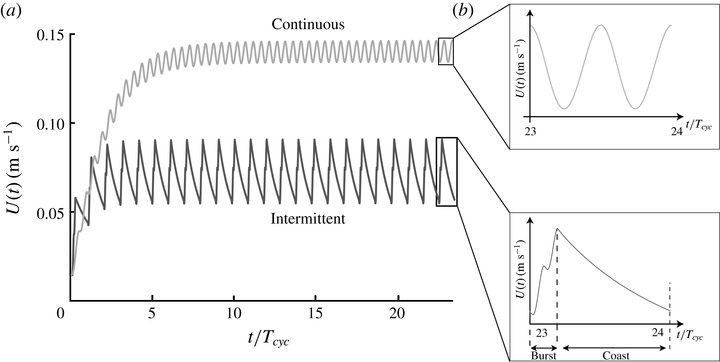
Figure 4(a) presents the swimming speed as a function of time for a representative continuous and intermittent swimmer. Both swimmers have the same Lighthill number of
 $Li=0.04$
, and are operating with the same frequency and amplitude of
 $f=1$
Hz and
 $A^{\ast }=0.7$
, respectively. The swimmers only differ in their duty cycle with the continuous swimmer using
 $DC=1$
and the intermittent swimmer using
 $DC=0.2$
. The swimmers start with an initial velocity of
 $U=0.1~\text{m}~\text{s}^{-1}$
and accelerate up to a steady-state condition after 10–20 cycles. Predictably, the intermittent swimmer has a lower mean speed at steady state than the continuous swimmer. Figure 4(b) shows the velocity as a function of time only over a single cycle for both swimmers. The continuous swimmer has the typical pattern observed in self-propelled studies (Borazjani & Sotiropoulos Reference Borazjani and Sotiropoulos2009; Moored & Quinn Reference Moored and Quinn2017) where there are two surging oscillations about the mean speed in a given cycle. This correlates with the two vortex shedding events and the two thrust peaks observed in oscillatory pitching motions. In contrast, the intermittent swimmer produces a different swimming pattern. During the bursting phase there are two surging oscillations as observed in the continuous swimmer case that are superposed onto an overall acceleration of the intermittent swimmer. When coasting the swimmer can be observed to decelerate nonlinearly as expected from a
 $U^{2}$
drag law with no oscillations in speed since the hydrofoil propulsor is static.
(a) Swimming speed as a function of the non-dimensional time normalized by the total cycle period for a characteristic continuous and a characteristic intermittent swimmer operating with
 $DC=0.2$
. (b) Swimming speed as a function of non-dimensional time over a single cycle of motion with the continuous swimmer in the top inlay and the intermittent swimmer in the bottom inlay.
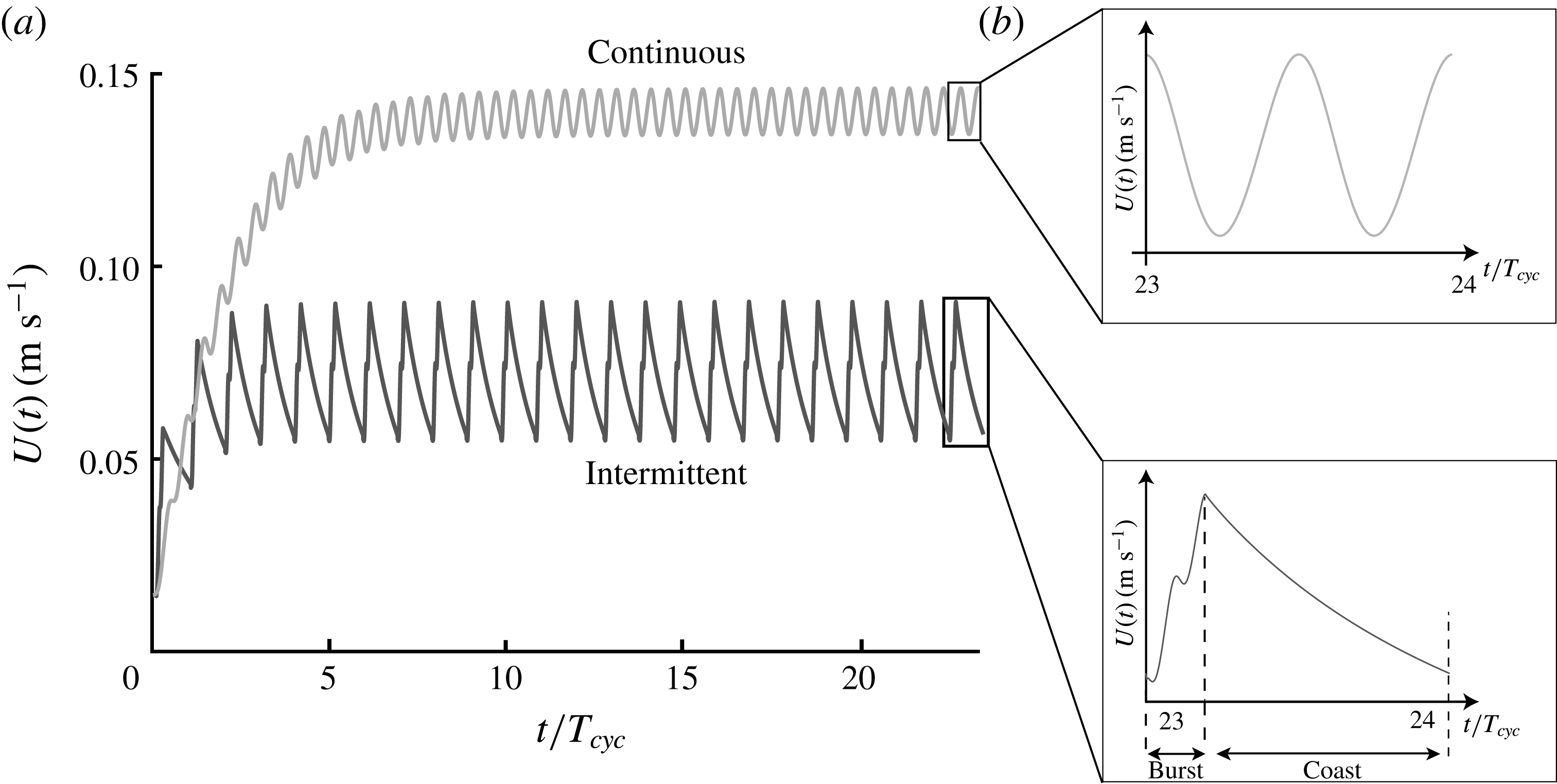
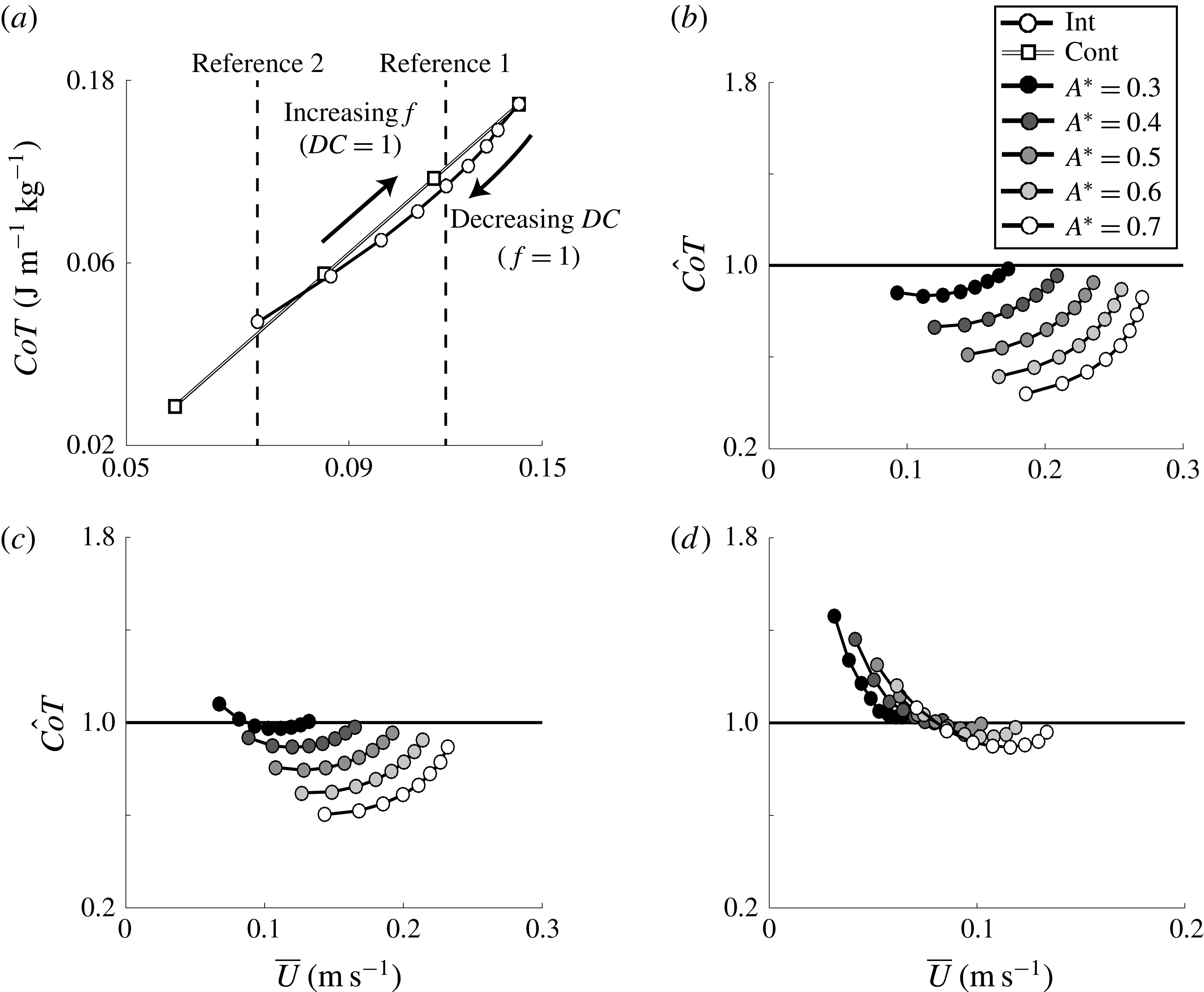
Figure 5(a) presents the
 $CoT$
as a function of the mean speed for a continuous and intermittent swimmer on a log–log scale. For both swimmers their amplitude of motion and Lighthill number are
 $A^{\ast }=0.7$
and
 $Li=0.4$
, respectively. The continuous swimmer has a fixed duty cycle of
 $DC=1$
and increases its oscillation frequency from
 $f=0.2$
–1 Hz. As the frequency of motion increases the mean speed increases linearly and the
 $CoT$
increases quadratically, which is made evident by the slope of the continuous swimmer line being equal to two on a log–log scale.
(a) Cost of transport as a function of the mean speed for a continuous and intermittent swimmer on a log–log scale. The swimming parameters are
 $A^{\ast }=0.7$
and
 $Li=0.4$
for both swimmers. The intermittent swimmer’s duty cycle ranges from
 $0.2\leqslant DC\leqslant 1$
with the lowest
 $DC$
associated with the lowest speed and vice versa. Normalized cost of transport as a function of the mean speed for three Lighthill numbers: (b)
 $Li=0.04$
, (c)
 $Li=0.08$
and (d)
 $Li=0.4$
. The intermittent swimmer’s duty cycle ranges from
 $0.2\leqslant DC\leqslant 0.9$
with the lowest
 $DC$
associated with the lowest speed and vice versa.
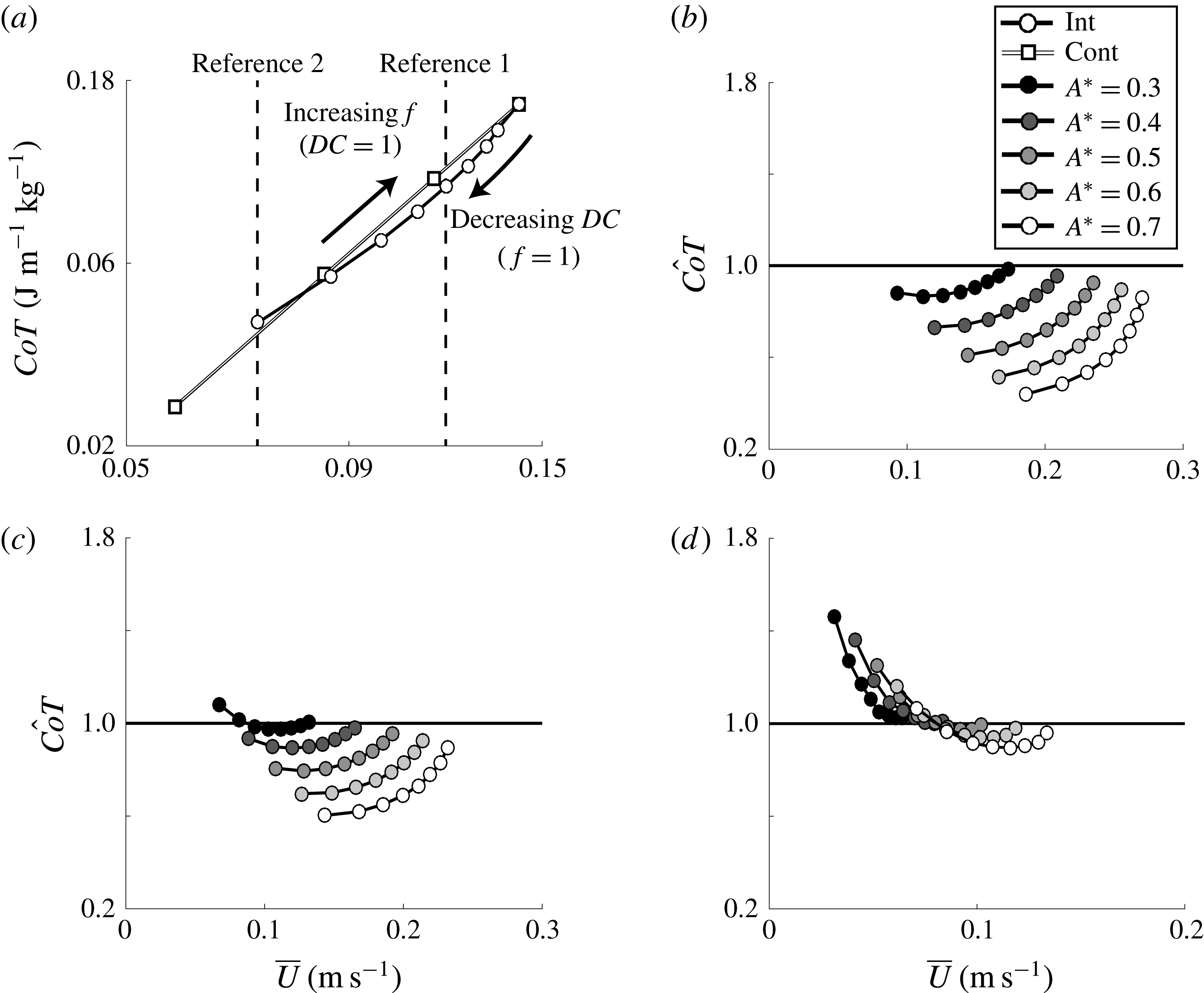
In contrast, the intermittent swimmer has a fixed frequency of
 $f=1$
Hz and decreases its duty cycle from
 $DC=1$
–0.2. At
 $DC=1$
and
 $f=1$
Hz, the intermittent and continuous swimmers are equivalent. When the duty cycle is decreased, the mean speed of the intermittent swimmer drops and consequently the
 $CoT$
decreases. It can be observed that there is a range of
 $DC$
where by using an intermittent gait swimmers can lower their
 $CoT$
while maintaining their swimming speed as compared to a continuous swimming gait (reference line 1), albeit with an increased oscillation frequency during the burst period. Additionally, there is a range of
 $DC$
where by using an intermittent gait costs more energy than continuous swimming at the same mean speed (reference line 2). Importantly, the energetically favourable regime of intermittent swimming is observed with potential flow simulations that do not compute the skin friction from the boundary layer, but instead rely on a drag law with a constant drag coefficient. This means that the observed benefit in the computations cannot be due to the viscous Bone–Lighthill boundary layer thinning hypothesis (Lighthill Reference Lighthill1971), which relies on an increase in the skin friction drag during oscillation to make intermittent swimming energetically favourable over continuous swimming. Instead, since a beneficial regime is still observed with potential flow computations then it must be due to an inviscid mechanism. This leads to a host of questions such as, how much of a benefit is observed? In what range of parameters does this benefit exist? What is the inviscid mechanism? How do the forces and energetics of intermittent swimming scale? What role does viscosity and the Bone–Lighthill mechanism play? The first four of these questions are examined in the current study while the last question is the subject of future work.
Figure 5(b–d) shows the normalized cost of transport as a function of the mean swimming speed for three different Lighthill numbers, that is,
 $Li=0.04,0.08$
and 0.4. For reference, low
 $Li$
represents highly streamlined swimmers with low non-dimensional fin loading and vice versa. Also, the the duty cycle ranges from
 $0.2\leqslant DC\leqslant 0.9$
with increasing
 $DC$
leading to higher speeds. If
 $\hat{CoT}>1$
then a continuous swimming gait is energetically beneficial. If
 $\hat{CoT}=1$
then both gaits are energetically equivalent. Finally, if
 $\hat{CoT}<1$
then an intermittent gait is energetically beneficial. Regardless of the
 $Li$
, choosing intermittent swimming is energetically more favourable as the amplitude of pitching increases. Additionally, the available energetic benefit from intermittent swimming becomes greater for decreasing
 $Li$
of swimmers. In fact, at
 $Li>0.4$
there is essentially a negligible energetic saving with only minute savings at very high duty cycles that can be garnered by switching to an intermittent gait. However, the
 $Li$
limit can be recast into a limit on the Reynolds number of swimming. Based on the drag coefficient of the laminar boundary layer on a flat plate
 $C_{D}=0.664\,Re_{l}^{-1/2}$
and the area ratio of
 $S_{wp}=8$
, then
 $Li=5.312\,Re^{-1/2}$
and intermittent swimming would produce no observable energetic benefits for
 $Re<175$
. At least this is an estimate for the inviscid benefit of intermittent swimming, but a Bone–Lighthill viscous benefit is not necessarily restricted in the same manner.
The lower bound on
 $Re$
where an intermittent benefit can be observed is reflected in biological studies. Larval northern anchovy uses continuous swimming whereas adult northern anchovy use an intermittent swimming mode (Weihs Reference Weihs1980; Müller et al.
Reference Müller, Stamhuis and Videler2000; Noda et al.
Reference Noda, Fujioka, Fukuda, Mitamura, Ichikawa and Arai2016). As larval northern anchovy reach 5 mm in length their typical Reynolds number during swimming is
 $Re\approx 100$
and coincidently the fish begin to swim intermittently.
For the lowest
 $Li$
and highest amplitude examined in this study, the
 $CoT$
reduction is as high as 60 %. In other words, a swimmer can choose to swim intermittently rather than continuously and save as much as 60 % of its energy per unit mass to travel a unit distance at the same speed. Importantly, unlike previous studies, this conclusion is obtained by fixing the drag coefficient for both bursting and coasting periods of swimming, meaning that the observed benefit is not due to the Bone–Lighthill boundary layer thinning hypothesis, but instead there is an inviscid mechanism that leads to the energy saving.
The simple scaling analysis presented in the introduction estimated that the Bone–Lighthill boundary layer thinning mechanism would lead to energy savings of 14 % and 19 % for low and high Reynolds number swimmers, respectively. Similar estimates of the energy savings from the inviscid mechanism are now 15 % and 60 % for low and high Reynolds numbers (
 $A^{\ast }=0.7$
). Now, by comparing the viscous and inviscid energy savings it is estimated that the inviscid mechanism will be comparable or dominate the energy savings of both low and high Reynolds number swimmers, respectively, that operate in a Reynolds number range of
 $O(10^{3})<Re<O(10^{6})$
.
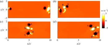
Evolution of the vorticity field of an intermittently pitching hydrofoil with
 $DC=0.2$
,
 $A^{\ast }=0.7$
and
 $Li=0.08$
. The evolution of the vortex wake is shown at times (a)
 $t/T_{cyc}=1/20$
, (b)
 $t/T_{cyc}=1/5$
, (c)
 $t/T_{cyc}=3/5$
and (d)
 $t/T_{cyc}=1$
.

3.2 Wake dynamics
Now that the inviscid energy benefit has been established, the characteristic wake topology for an intermittent swimmer is detailed. Figure 6 shows the evolution of the vorticity field throughout a cycle for an intermittent swimmer with
 $DC=0.2$
. The distribution of positive (anti-clockwise) and negative (clockwise) vorticity are represented with white and black, respectively. There is no near wake at the beginning of the burst period since previous wake structures have advected multiple chord lengths away (figure 6
a). Over each bursting period, four vortices are shed; one starting vortex (vortex A), two vortices are shed as the hydrofoil changes direction (vortices B and C) and one weak stopping vortex (D) (figure 6
b). Vortices B and C are stronger and form a pair as they travel downstream (figure 6
c,d). Due to mutual induction, vortices B and C advect downstream faster than vortices A and D. On the other hand, vortex A induces some vorticity from vortex B to be left behind in its downstream propagation (figure 6
d). The evolution of the vortex wake shown in figure 6 for
 $DC=0.2$
is characteristic of all of the duty cycles examined of intermittent swimmers. The vortex group A–D is repeated for each oscillation cycle with the spacing between vortex groups being reduced as the
 $DC$
increases.
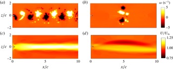
The vorticity field of hydrofoils pitching with
 $A^{\ast }=0.7$
and
 $Li=0.08$
at (a)
 $DC=1$
and (b)
 $DC=0.2$
. Time-averaged velocity fields of (c) the continuous and (d) the intermittent gait at a mean speed of
 $\overline{U}=0.14~\text{m}~\text{s}^{-1}$
.

The induced velocities among the three strong vortices shed during a bursting period of an intermittent gait (figure 7
b) leads to an asymmetry in the time-averaged velocity field. Figure 7(c,d) shows the comparison of the time-averaged
 $x$
-velocity field of a continuously pitching hydrofoil (
 $f=0.58$
Hz and
 $DC=1$
) with its intermittently pitching counterpart swimming at the same mean speed of
 $\overline{U}=0.14~\text{m}~\text{s}^{-1}$
. For the continuous swimmer, the symmetrically shed vortices create a reverse von Kármán street, which time averages to a single-core jet aligned in the streamwise direction. For the intermittent swimmer, in the near wake (
 $x/c\leqslant 1$
), the vortices are shed in a similar manner to a classic reverse von Kármán street creating a time-averaged momentum jet aligned in the streamwise direction. In the far wake (
 $x/c\geqslant 1$
), the three strong vortices evolve into two pairs with one pair inducing a velocity in the downstream direction while the other induces a velocity upstream. In the time-averaged sense this creates a momentum surplus and deficit branch that are parallel to each other for
 $2\leqslant x/c\leqslant 8$
. The momentum jet is observed to also have an asymmetry suggesting that there is finite time-averaged lateral force produced by the swimmer.
3.3 Scaling laws of intermittent swimming
Here the scaling of the forces and energetics of intermittent swimming with the swimming parameters will be considered. Of prime importance are the scaling of the mean swimming speed and the cost of transport, which are inherently linked to the scaling of the mean thrust production and mean power consumption of a swimmer (Moored & Quinn Reference Moored and Quinn2017). Here, we will show that a simple scaling of the thrust and power with the duty cycle can be used to transform the intermittent swimming problem into a continuous swimming problem. Then previously derived scaling relations for continuous swimming will be shown to seamlessly apply to scaling the transformed thrust and power.
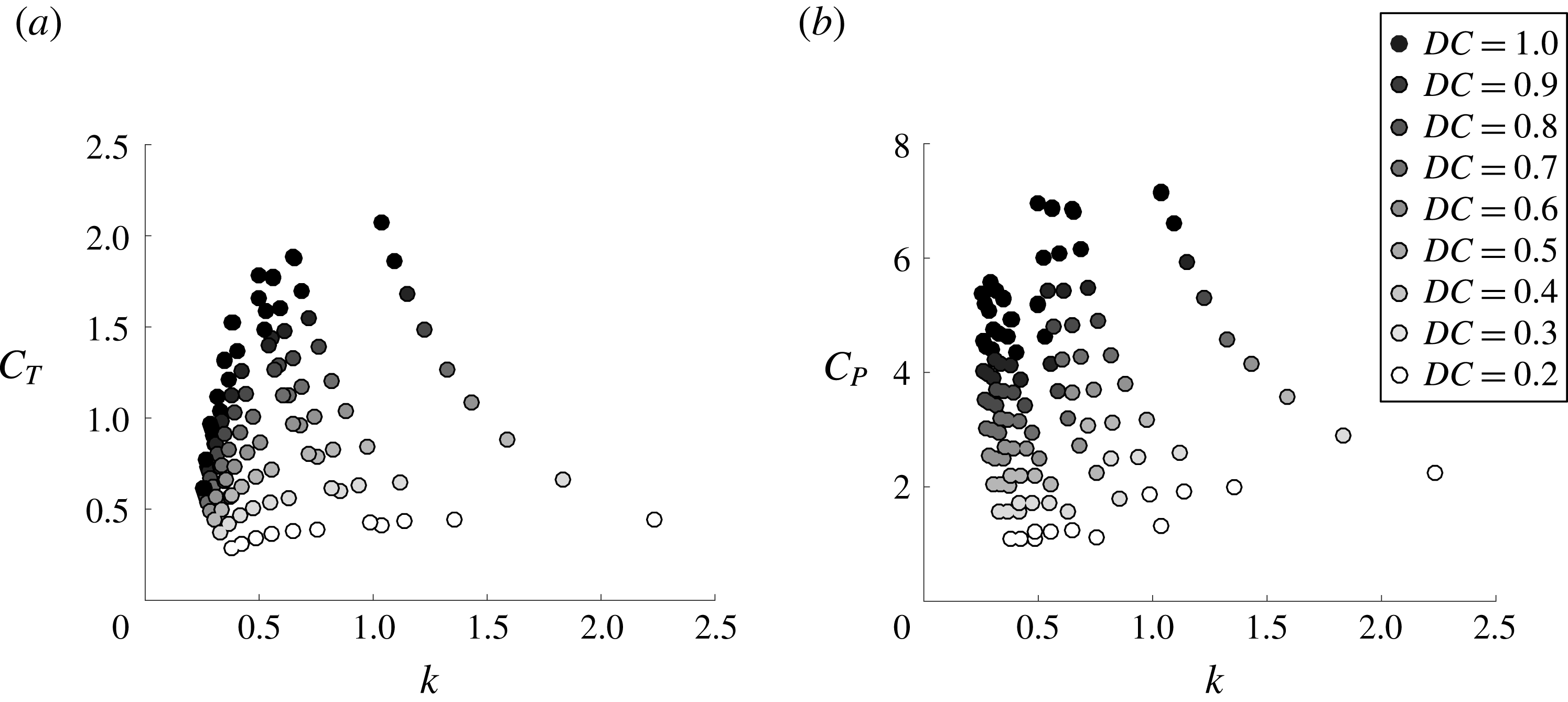
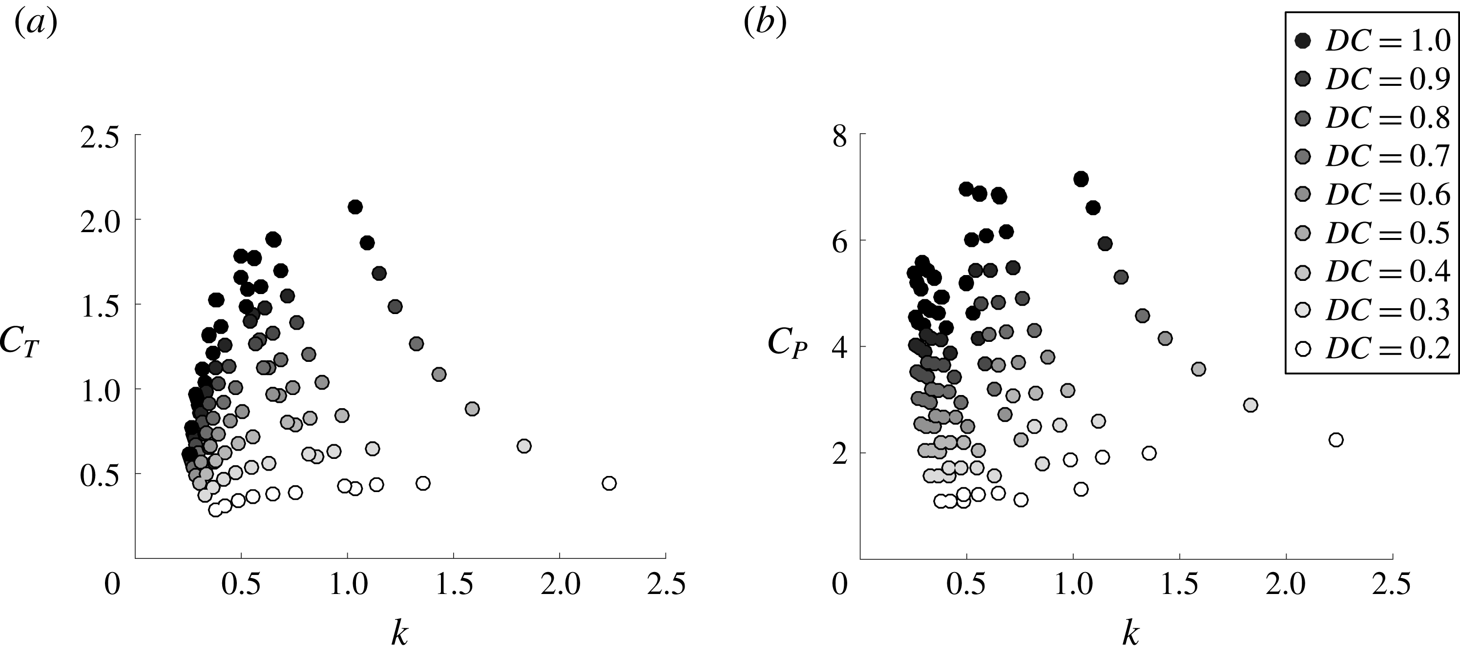
Figure 8(a) shows the thrust coefficient for swimmers as a function of the reduced frequency for various duty cycles ranging from
 $0.2\leqslant DC\leqslant 1$
. The mean thrust used in the definition of the thrust coefficient is averaged over an entire cycle, that is, the combined bursting and coasting periods. For a given duty cycle, the thrust is observed to increase with an increase in the reduced frequency. Similarly, for a fixed reduced frequency the thrust increases with an increase in the duty cycle. Figure 8(b) presents the power coefficient as a function of the reduced frequency. Like the thrust coefficient, the power is seen to increase with increasing reduced frequency and duty cycle. The thrust and power both show a large range of values with the variation of the parameters
 $f,Li,DC$
, and
 $A^{\ast }$
.
Mean (a) thrust coefficient and (b) power coefficient as a function of reduced frequency.
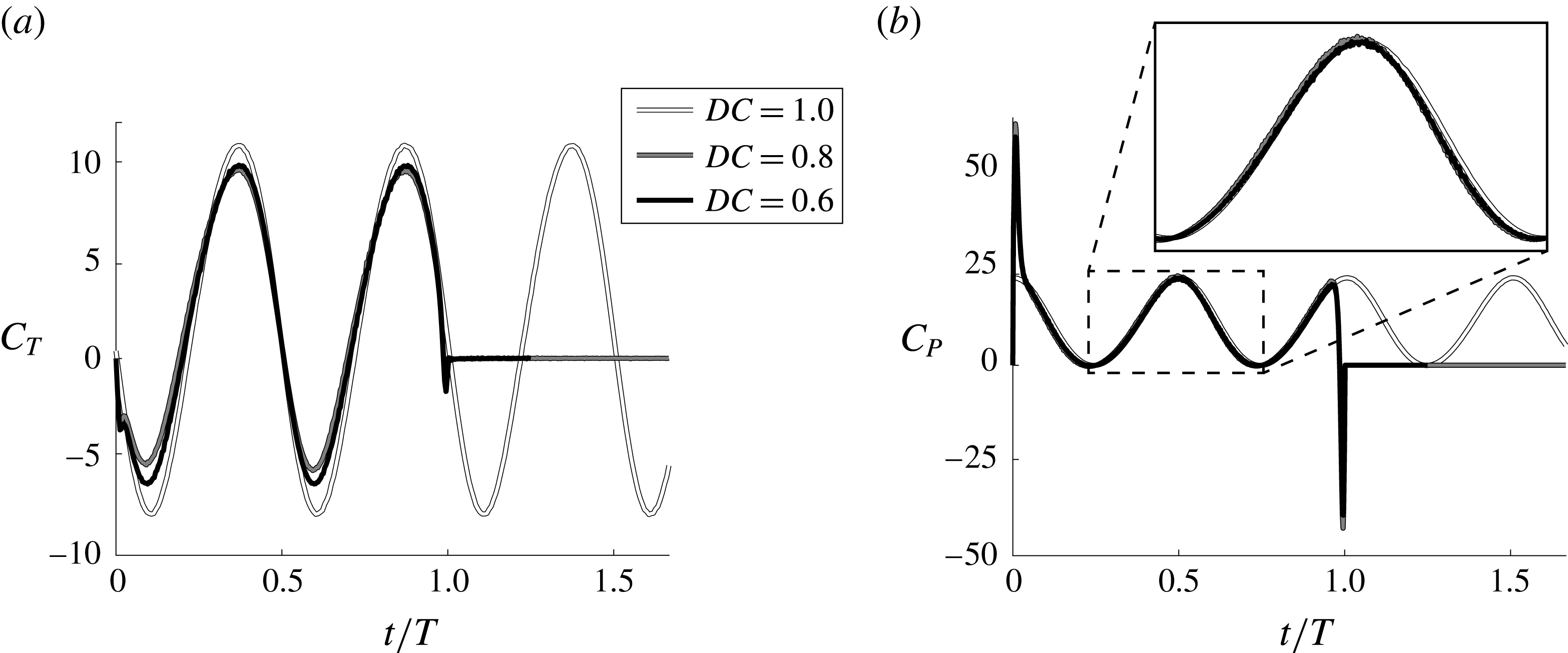
To gather more insight into how the thrust and power scale with the kinematic parameters, the instantaneous thrust and power are presented in figure 9. The thrust for the continuous swimmer shows two characteristic peaks that are associated with the peak angular accelerations that occur during a cycle and the subsequent shedding of two vortices per oscillation cycle (figure 7
a). Similarly, the intermittent swimmers with
 $DC=0.6$
and 0.8 show two peaks in thrust that are associated with the shedding of the two strongest vortices that form during an intermittent swimming cycle (vortices B and C in § 3.2). In contrast, there are two small troughs in the instantaneous thrust at the beginning and end of the burst period that are associated with shedding of the starting and stopping vortices (vortices A and D in § 3.2) that occur from the high accelerations at the beginning and end of the burst period. As the duty cycle is lowered from
 $DC=1$
the peaks and troughs of the instantaneous thrust are attenuated with the troughs showing large reductions in their peak drag. By considering only the bursting period, the mean thrust actually rises as the duty cycle decreases. However, when considering the mean thrust over the entire cycle, this small rise in thrust during the bursting period is overcome by the effectively zero thrust throughout the coasting phase. In this respect, a better comparison of the mean thrust among different duty cycles of swimming would average the thrust only over the bursting period,
 $C_{T,burst}$
. The mean thrust over the bursting period and the mean thrust over the entire cycle are simply connected as,
 $$\begin{eqnarray}\displaystyle C_{T,burst}=\frac{C_{T}}{DC}. & & \displaystyle\end{eqnarray}$$
The major effect of the thrust reduction with decreasing duty cycle can then be accounted for by scaling the mean thrust over the entire cycle with the duty cycle as in (3.1).
Instantaneous (a) thrust coefficient and (b) power coefficient for three duty cycles of
 $DC=0.6$
, 0.8 and 1. The frequency, amplitude and Lighthill number are
 $f=1$
Hz,
 $A^{\ast }=0.7$
and
 $Li=0.04$
, respectively, for all of the duty cycles.
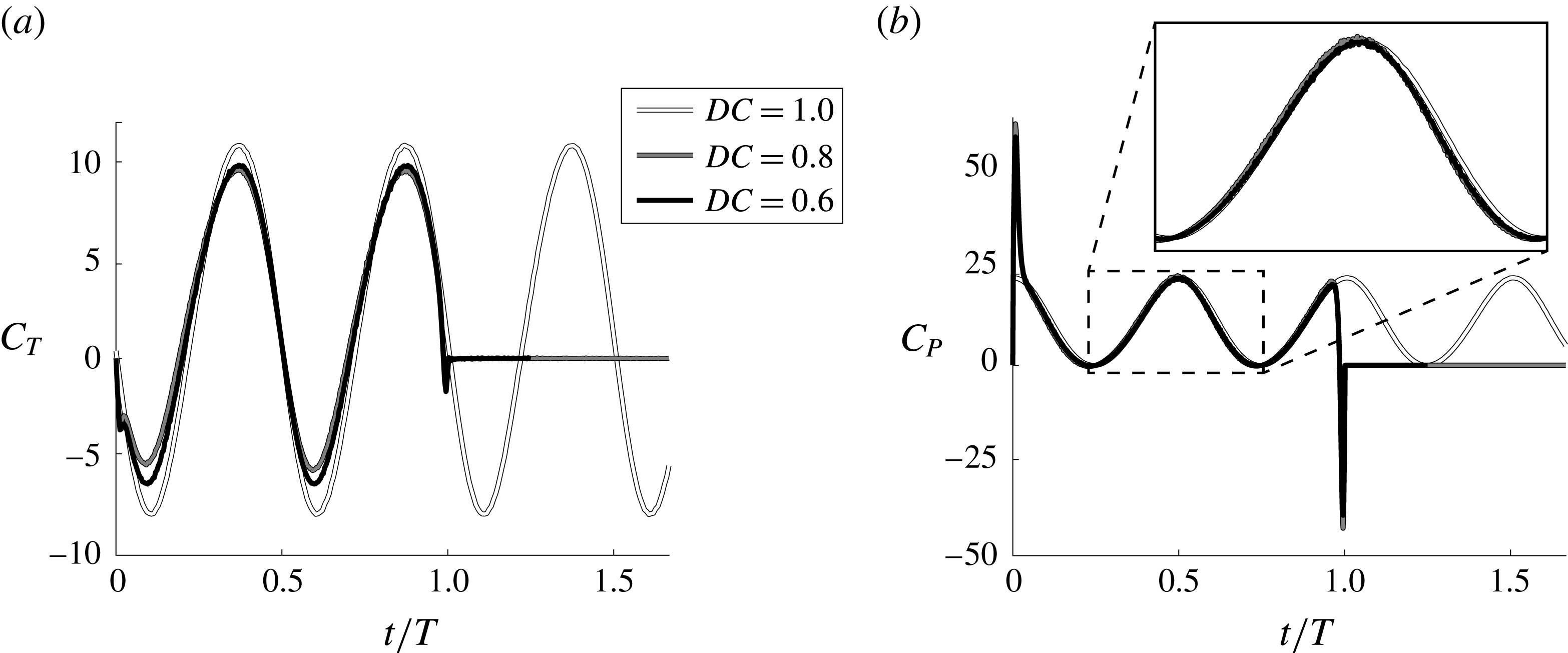
In figure 9(b) the continuous swimmer is seen to have two peaks in power over an oscillation cycle that occurs near the peak angular velocity of the pitching hydrofoil. In contrast, the intermittent swimmers have a prominent peak and trough in the power consumption at the beginning and end of the bursting period in accordance with the high accelerations at those times, however, they essentially cancel and provide a negligible contribution to the mean power. As the duty cycle decreases the instantaneous power is seen to be amplified only slightly over the bursting period and consequently the mean power over the bursting phase is observed to increase minutely for this case. The instantaneous power also shows zero power consumption during the coasting phase since the pitching hydrofoil has no angular velocity during that phase. Like the thrust, this leads to a reduction in the mean power over the entire cycle, which can be accounted for by averaging the power over the bursting period or equivalently by scaling the power with the duty cycle,
 $$\begin{eqnarray}\displaystyle C_{P,burst}=\frac{C_{P}}{DC}. & & \displaystyle\end{eqnarray}$$
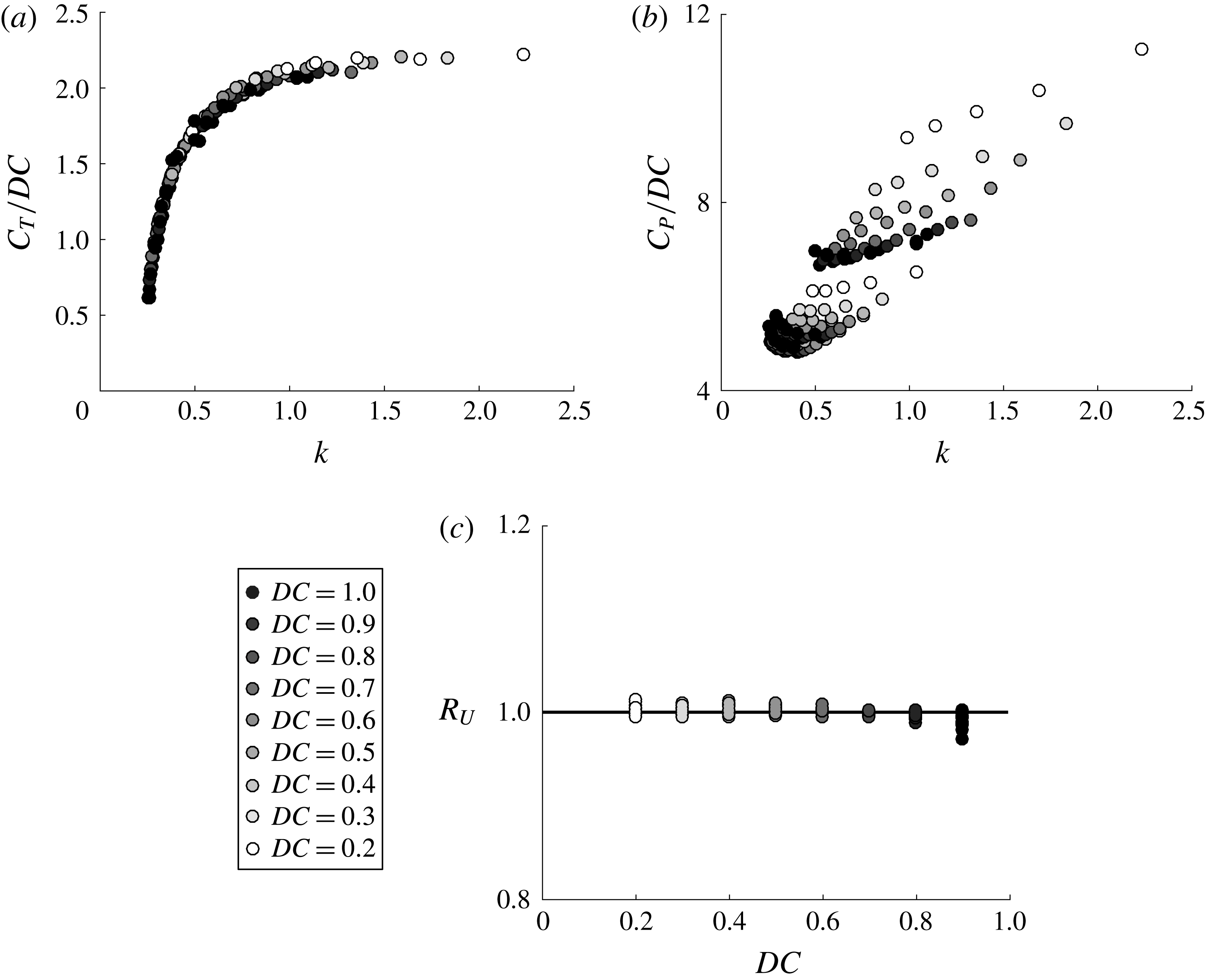
Now, the thrust and power coefficients are scaled in accordance with (3.1) and (3.2) and presented in figure 10(a,b). The thrust data have now collapsed to a line while the power data are more compact, but there is still stratification in the data. What is particularly striking is that the data now resemble self-propelled data from only continuous swimmers (Moored & Quinn Reference Moored and Quinn2017). This shows that by applying the simple scalings in (3.1) and (3.2), the intermittent swimming problem has been transformed into a continuous swimming problem. It is now hypothesized that previously derived scaling relations for self-propelled continuous swimmers can account for the physics of the transformed problem.
(a) Mean scaled thrust coefficient as a function of the reduced frequency. (b) Mean scaled power coefficient as a function of the reduced frequency. (c) Ratio of the predicted mean speed from the scaling relation to the mean speed from the simulations as a function of
 $DC$
.

Moored & Quinn (Reference Moored and Quinn2017) examined the inviscid scaling laws of a self-propelled pitching hydrofoil combined with a virtual body (same model as the current study). The numerical results were compared with the exact scaling relations from Garrick’s theory (Garrick Reference Garrick1936). Surprisingly, the linear theory was found to capture the scaling behaviour of the mean thrust from the nonlinear numerical results (Moored & Quinn Reference Moored and Quinn2017). Now, a generalized scaling relation for mean thrust of an intermittent swimmer is determined by applying the duty cycle transformation to the thrust relation proposed by Moored & Quinn (Reference Moored and Quinn2017),
 $$\begin{eqnarray}\displaystyle \frac{C_{T}(k)}{DC}=c_{1}-c_{2}\,w(k), & & \displaystyle\end{eqnarray}$$
where
 $$\begin{eqnarray}\displaystyle w(k)=\frac{3F(k)}{2}+\frac{F(k)}{\unicode[STIX]{x03C0}^{2}k^{2}}-\frac{G(k)}{2\unicode[STIX]{x03C0}k}-[F(k)^{2}+G(k)^{2}]\left(\frac{1}{\unicode[STIX]{x03C0}^{2}k^{2}}+\frac{9}{4}\right). & & \displaystyle\end{eqnarray}$$
Here
 $F$
and
 $G$
are the real and imaginary parts of Theodorsen’s lift deficiency function (Theodorsen Reference Theodorsen1935) and
 $c_{1}$
and
 $c_{2}$
are coefficients that are to be determined from the data. The wake function
 $w(k)$
is specified for a pitching axis about the leading edge.
From this relation, by plotting
 $C_{T}/DC$
on a vertical axis and
 $k$
on a horizontal axis the data should collapse to a line that is only a function of
 $k$
. This is precisely what is observed in figure 10(a), which confirms that the scaling relation (3.3) captures the proper physics.
The physical meaning of the first and second terms on the right-hand side of (3.3) can be directly interpreted from Garrick’s theory where they represent the added-mass and circulatory streamwise forces, respectively. In fact, for pitching about the leading edge, the circulatory term is always drag inducing for all
 $k$
and the added-mass term is always thrust producing. Consequently, as the reduced frequency of a swimmer is increased, it will increase the ratio of the thrust-producing added-mass forces relative to the drag-inducing circulatory forces.
Through a simple algebraic extension the thrust scaling relation can be used to calculate the self-propelled mean swimming speed of an intermittent swimmer. By recognizing that during steady-state swimming the mean thrust is balanced by the mean drag then the thrust relation can be combined with the drag law (2.1) to determine the mean swimming speed,
 $$\begin{eqnarray}\displaystyle \overline{U}_{scale}=fA\sqrt{2\,DC\frac{C_{T}^{cont}(k)}{Li}}. & & \displaystyle\end{eqnarray}$$
To make this scaling relation predictive only two simulations would need to be run to determine the coefficients in (3.3). Here, the coefficients are determined to be
 $c_{1}=0.536$
and
 $c_{2}=2.3$
by minimizing the squared residuals with the entire set of simulation data. Now, the scaling relation prediction can be directly assessed against the data gathered from the numerical simulations by forming a ratio of the mean swimming speeds as,
 $R_{U}=\overline{U}_{scale}/\overline{U}_{sim}$
. If this ratio is equal to one then the scaling relation provides an exact prediction of the mean speed from the nonlinear simulations. Figure 10(c) presents the ratio of swimming speeds as a function of the duty cycle. It is evident that the scaling relation provides an excellent prediction of the mean swimming speed for an intermittent swimmer where the mean speed scaling prediction is within 3 % of its full-scale value from the simulations. Here the drag law used in the simulations was prescribed a priori, however, the key to predicting the swimming speed is to have the proper thrust scaling relation, which is not prescribed a priori in the simulations. This result confirms the algebraic extension from thrust to swimming speed and that the thrust scaling is accurate for a range of reduced frequencies.
The scaled mean power coefficient as a function of
 $\unicode[STIX]{x1D719}_{1}$
and
 $\unicode[STIX]{x1D719}_{2}$
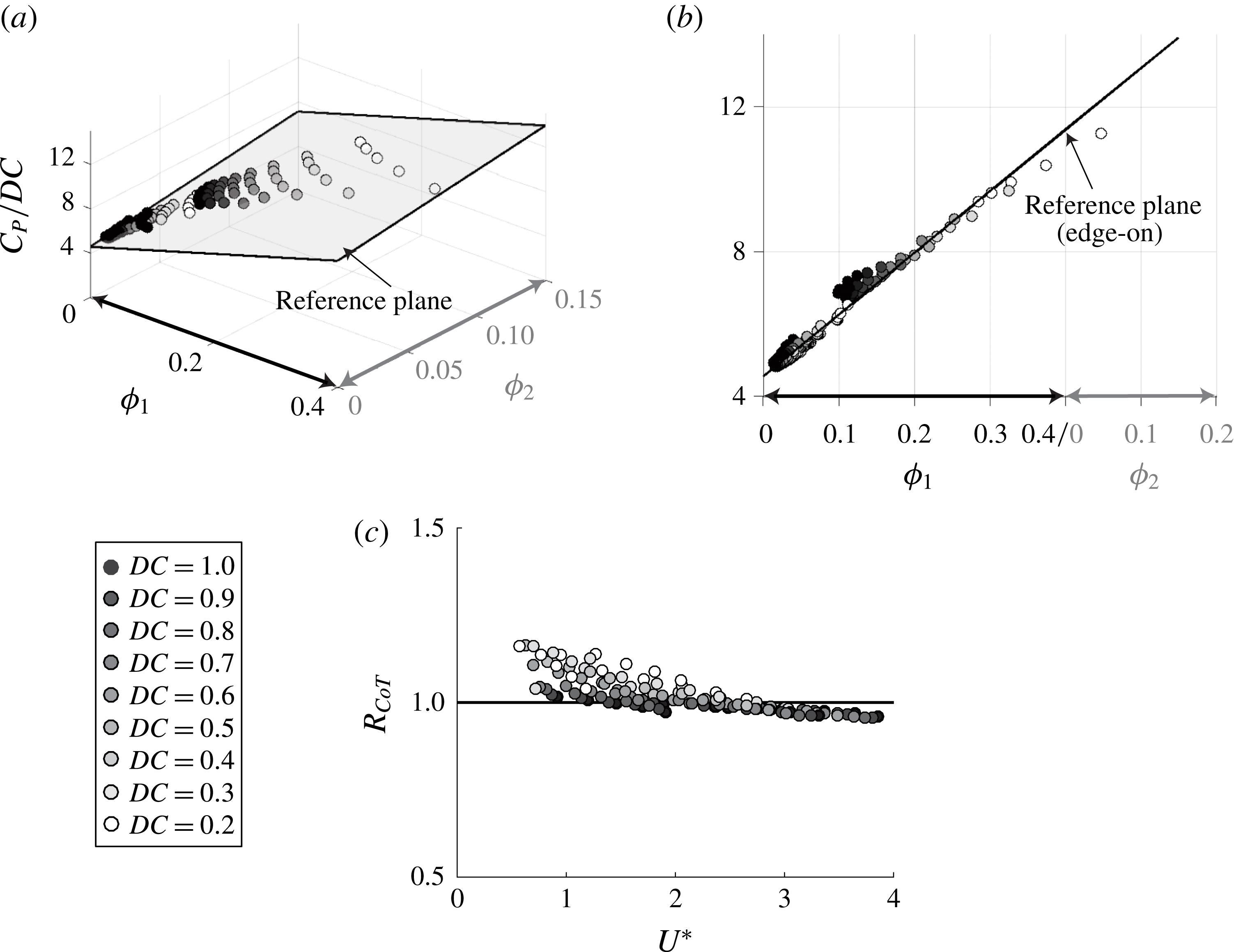
from (a) a perspective view and (b) an ‘edge-on’ view of the reference plane. (c) Ratio of the cost of transport predicted from the scaling laws to the actual computational data as a function of the duty cycle.

In contrast to the thrust scaling relation, Moored & Quinn (Reference Moored and Quinn2017) determined that Garrick’s linear theory did not accurately capture the scaling trends in the power coefficient for their nonlinear simulation data. They argued that linear theory needed to be augmented by two nonlinear corrections that are not accounted for in linear theory due to its assumptions. The power scaling relation for continuous swimming proposed by Moored & Quinn (Reference Moored and Quinn2017) is then generalized for intermittent motions by applying the duty cycle transformation to the scaling relation,
 $$\begin{eqnarray}\displaystyle \frac{C_{P}(k,St)}{DC}=c_{3}+c_{4}\,\frac{St^{2}}{k}\left(\frac{k^{\ast }}{k^{\ast }+1}\right)+c_{5}\,St^{2}k^{\ast }. & & \displaystyle\end{eqnarray}$$
Here the modified reduced frequency is
 $k^{\ast }=k/(1+4St^{2})$
. Following Moored & Quinn (Reference Moored and Quinn2017), the first term represents the added-mass power directly from linear theory, the second term represents the power from the large-amplitude separating shear layer and the third term represents the power from the proximity of the trailing-edge vortex. Here the coefficients
 $c_{3}$
,
 $c_{4}$
and
 $c_{5}$
are to be determined from the numerical data. By examining (3.6), if
 $C_{P}/DC$
is plotted as a function of
 $\unicode[STIX]{x1D719}_{1}=(St^{2}/k)(k^{\ast }/(k^{\ast }+1))$
and
 $\unicode[STIX]{x1D719}_{2}=St^{2}k^{\ast }$
in a three-dimensional graph, then the numerical data should collapse to a plane. Figure 11(a) shows a perspective view of the three-dimensional data and figure 11(b) shows an ‘edge-on’ view of the data with a reference plane. It can be seen that there is an excellent collapse of the scaled power coefficient data to a plane. This confirms that the continuous swimming scaling relations account for the physics of intermittent swimming once the intermittent transformation is applied.
The power coefficient scaling relation can be extended through simple algebra to calculate a scaling relation for the cost of transport giving
 $$\begin{eqnarray}\displaystyle CoT_{scale}=\frac{\unicode[STIX]{x1D70C}S_{p}f^{2}A^{2}}{m}DC\,C_{P}(k,St). & & \displaystyle\end{eqnarray}$$
To make this scaling relation predictive, only three simulations would need to be run to determine the three coefficients,
 $c_{3}$
,
 $c_{4}$
and
 $c_{5}$
. Here, the coefficients are determined to be
 $c_{3}=4.551$
,
 $c_{4}=17.08$
and
 $c_{5}=16.86$
by minimizing the squared residuals for the entire data set. Subsequently, the ratio of the predicted cost of transport compared to the cost of transport from the simulations can be formed as
 $R_{CoT}=CoT_{scale}/CoT_{sim}$
. Figure 11(c) shows the ratio of the cost of transports as a function of the non-dimensional speed where
 $R_{CoT}=1$
represents a perfect scaling prediction of the actual simulation data. The scaling prediction is observed to predict the actual cost of transport to within 18 % of its full-scale value. This confirms the algebraic extension of the power coefficient scaling to the cost of transport and that the power scaling relation is accurate for a range of
 $k$
and
 $St$
.
3.4 Inviscid energy saving mechanism
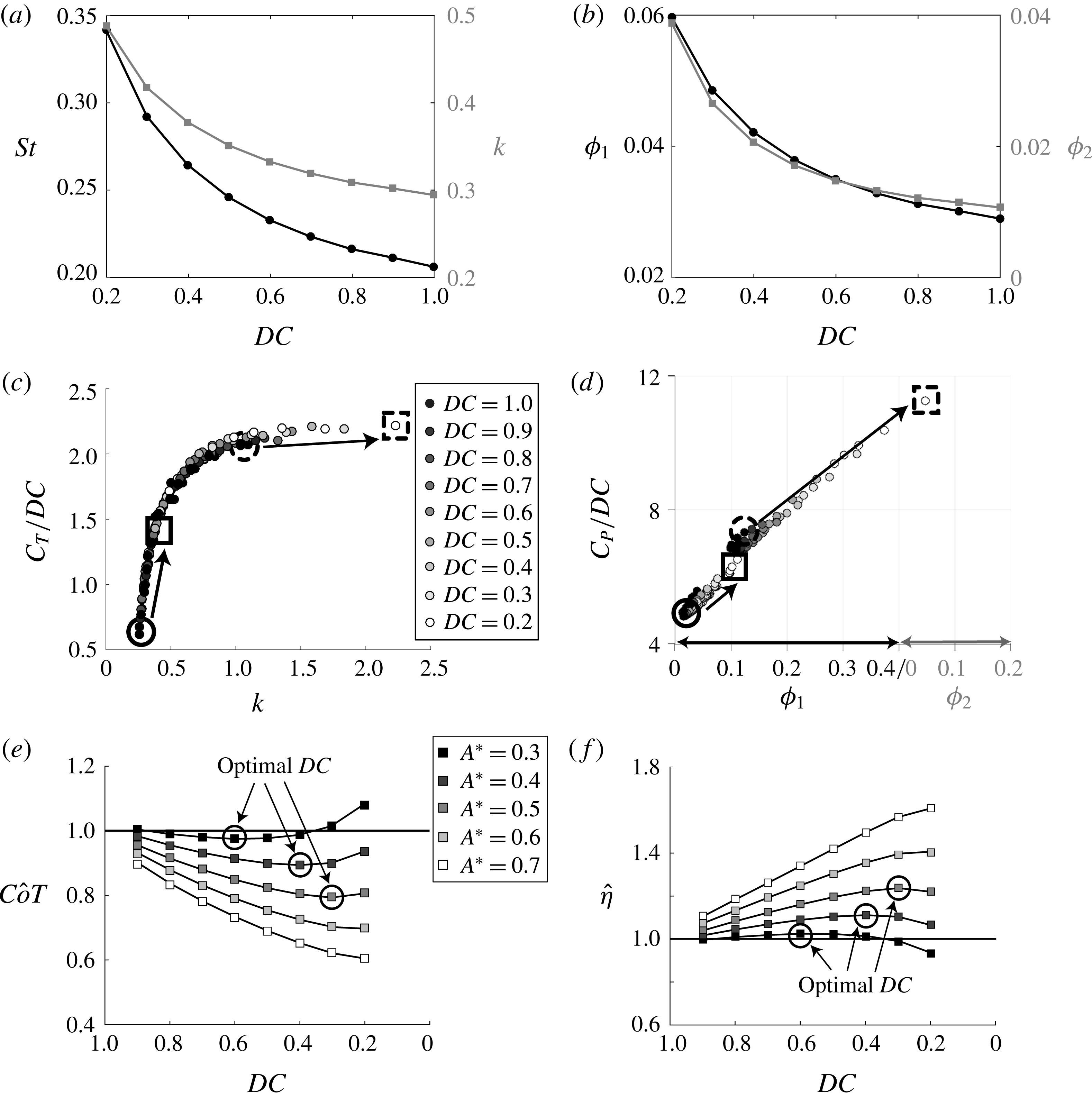
Section 3.1 presented that an intermittent swimmer can save energy compared to a continuous swimmer when swimming at the same mean speed in an inviscid environment. Now, the scaled data from § 3.3 can be examined to elucidate the inviscid mechanism behind the energetic benefit as well as the limits of the energy savings.
(a) Strouhal number and reduced frequency as a function of the duty cycle for
 $A^{\ast }=0.7$
and
 $Li=0.08$
. (b) Large-amplitude separating shear layer term and the vortex proximity term as a function of the duty cycle for
 $A^{\ast }=0.7$
and
 $Li=0.08$
. (c) Scaled thrust as a function of reduced frequency. (d) Scaled power as a function of
 $\unicode[STIX]{x1D719}_{1}$
and
 $\unicode[STIX]{x1D719}_{2}$
. (e) Normalized cost of transport as a function of duty cycle,
 $Li=0.08$
. (f) Normalized efficiency as a function of duty cycle,
 $Li=0.08$
. The black circles indicate the optimal duty cycle for each
 $A^{\ast }$
.

When a swimmer switches from continuous to intermittent swimming and reduces its duty cycle it will consequently swim slower (figure 5), which will result in a rise in
 $k$
and
 $St$
. As expected, figure 12(a) presents a monotonic increase in the reduced frequency and Strouhal number as the
 $DC$
decreases for
 $A^{\ast }=0.7$
and
 $Li=0.08$
. At the same time, the large-amplitude separating shear layer term,
 $\unicode[STIX]{x1D719}_{1}=(St^{2}/k)(k^{\ast }/(k^{\ast }+1))$
, and the vortex proximity term,
 $\unicode[STIX]{x1D719}_{2}=St^{2}k^{\ast }$
, also show a monotonic increase with decreasing duty cycle (figure 12
b). Since
 $k$
,
 $\unicode[STIX]{x1D719}_{1}$
, and
 $\unicode[STIX]{x1D719}_{2}$
all increase monotonically with decreasing
 $DC$
the scaled thrust and power coefficients are observed to also increase monotonically with decreasing
 $DC$
(figure 12
c,d). However, the rate of change of increase is different for scaled thrust and power coefficients as the duty cycle decreases. This difference determines whether choosing intermittent swimming saves energy over continuous swimming or not.
To examine this more closely a high-amplitude low
 $Li$
swimmer and a low-amplitude high
 $Li$
swimmer are compared in terms of their scaled thrust and power data. A swimmer with
 $A^{\ast }=0.7$
,
 $Li=0.04$
, and
 $DC=1$
is highlighted on both the scaled thrust and power graphs by solid black circles in figure 12(c,d). When the swimmer reduces its duty cycle to
 $DC=0.2$
, its new scaled thrust and power conditions are highlighted on the graphs by solid black squares. It is observed that the thrust coefficient rises by 113 % while the power coefficient rises by only 8 %. For this high-amplitude low
 $Li$
swimmer, the rise in thrust outweighs the rise in power and the propulsive efficiency therefore increases by 98 %. There is a second swimmer with
 $A^{\ast }=0.3$
,
 $Li=0.4$
and
 $DC=1$
that is highlighted on both the scaled thrust and power graphs by dashed black circles. The swimmer then lowers its duty cycle to
 $DC=0.2$
and its new scaled thrust and power conditions are highlighted on the graphs by dashed black squares. For this low-amplitude high
 $Li$
swimmer, it is observed that when the
 $DC$
decreases the thrust coefficient only rises by 7 % while the power coefficient rises by 54 % which results in a 30 % drop in efficiency.
To connect the energy saving results presented in § 3.1 with the optimum duty cycle behaviour, the normalized efficiency and cost of transport (see (2.25)) are plotted as a function of the duty cycle (figure 12
e,f). If
 $\hat{\unicode[STIX]{x1D702}}>1$
intermittent swimming is more efficient than the continuous swimming and vice versa. Similarly, if
 $\hat{CoT}<1$
intermittent swimming uses less energy than the continuous swimming and vice versa. Furthermore, the efficiency and cost of transport can be directly linked at the same mean speed by recognizing that during steady-state swimming the mean thrust and drag must balance, which leads to
 $\overline{T}=1/2\,C_{d}\unicode[STIX]{x1D70C}S_{p}U^{2}$
and
 $$\begin{eqnarray}\displaystyle CoT=\frac{\overline{P}}{m\overline{U}}=\frac{\overline{P}\overline{T}}{m\overline{U}\overline{T}}=\frac{\frac{1}{2}C_{d}\unicode[STIX]{x1D70C}U^{2}}{m\,\unicode[STIX]{x1D702}}=\frac{\text{const.}}{\unicode[STIX]{x1D702}}. & & \displaystyle\end{eqnarray}$$
This relation shows that at the same mean speed,
 $CoT\propto 1/\unicode[STIX]{x1D702}$
and figure 12(f) is just the inverse of figure 12(e). It can be observed that there is an optimal duty cycle marked by the black circles in figure 12(e,f) that minimizes the normalized cost of transport and maximizes the normalized efficiency simultaneously. Additionally, the optimal duty cycle decreases with increasing amplitude of motion.
Overall, high energy savings can occur when a continuous swimmer has a sufficiently low reduced frequency in the range of
 $0.25\leqslant k\leqslant 1$
such that by reducing their
 $DC$
will result in a thrust increase that will outweigh their power increase. Consequently, their efficiency will increase and their cost of transport will decrease. If a continuous swimmer has a high reduced frequency of
 $k>1$
then lowering their
 $DC$
will result in a power increase that outweighs their thrust increase, which will lead to lower efficiency and higher cost of transport.
Now, the inviscid mechanism behind the energy savings observed in intermittent swimming can be described as a Garrick mechanism since it relies on the trade-off between the added-mass and circulatory forces, which is predicted by Garrick’s theory (Garrick Reference Garrick1936). Importantly, the Garrick mechanism leads to an improvement in the propulsive efficiency that is independent of the Bone–Lighthill viscous mechanism. It is also expected that the general results presented in this study would apply to three-dimensional swimmers given that the added-mass and circulatory forces acting on pitching wings is similar in two and three dimensions (Dewey et al. Reference Dewey, Boschitsch, Moored, Stone and Smits2013). However, future work will extend this study to fully examine three-dimensional and viscous effects on the performance and wake topologies of intermittent swimmers. Further extensions that consider the effects of flexibility may be informed by recent theoretical work on the subject (Moore Reference Moore2014, Reference Moore2015, Reference Moore2017) and are being pursued.
4 Conclusion
The performance and wake structures of a self-propelled swimmer modelled as a combination of a virtual body and an intermittently pitching hydrofoil are examined by using an inviscid boundary element method. Intermittent swimming is characterized by a wake topology consisting of four vortices shed per pitching cycle and an asymmetric time-averaged jet structure with both momentum surplus and deficit branches. The mean thrust and power coefficients are shown to scale with the
 $DC$
, which can be used to transform the intermittent swimming problem into a continuous swimming problem. Previous continuous swimming scaling relations are generalized to include intermittent swimming, and extended to calculate the mean swimming speed and the cost of transport. These relations are shown to become predictive by tuning a few coefficients with a handful of simulations. In the current study, the mean speed and cost of transport are predicted to within 3 % and 18 % of their full-scale values by using these relations.
In contrast to previous studies, a drag law is prescribed for the virtual body that has a constant drag coefficient, that is, it does not depend upon whether a swimmer is bursting or coasting. Under these conditions it is discovered that swimming intermittently can save as much as 60 % of the energy it takes to swim continuously at the same mean speed even in an inviscid environment. This finding shows that in addition to the viscous Bone–Lighthill boundary layer thinning mechanism proposed by Lighthill (Reference Lighthill1971) there is another inviscid ‘Garrick’ mechanism behind the energy savings of intermittent swimming. This mechanism is determined to lead to an improvement in the propulsive efficiency of a swimmer by altering the ratio of its added-mass thrust-producing forces relative to its circulatory drag-inducing forces. A key discovery is that this occurs in self-propelled swimming by reducing the duty cycle of an intermittent swimmer, and consequently increasing its reduced frequency. Additionally, the energy saving potential is shown to be the greatest for low Lighthill number continuous swimmers using high-amplitude motions, where a low Lighthill number represents a swimmer with a highly streamlined body. This occurs during self-propelled locomotion since these parameters lead to low reduced frequency swimming, which has the greatest potential for a large bursting period thrust enhancement. In contrast, the energy savings of intermittent swimming switches to an additional energetic cost over continuous swimming when the force production of the swimmer is dominated by added-mass forces. Under this condition during the bursting period there is a negligible thrust enhancement benefit and instead there is a large additional power cost as the swimmer’s duty cycle is reduced.
Acknowledgement
This work was funded by the Office of Naval Research under Program Director Dr B. Brizzolara, MURI grant no. N00014-14-1-0533.