1. Introduction and background
Surface roughness is found in abundance in natural environments and plays an important role in a variety of practical and engineering applications. Nevertheless, while rough walls are of great importance, they are much less well understood than their smooth-wall counterparts (Jimenez Reference Jimenez2004). It is well established that, compared with the law of the wall for smooth walls, any rough surface morphology results in a downward shift in the logarithmic portion of the velocity profile. For a rough-wall boundary layer, the velocity profile in the log region can be expressed as
 $$\begin{eqnarray}U^{+}=\frac{1}{{\it\kappa}}\ln \left(\frac{y-d}{y_{0}}\right)\equiv \frac{1}{{\it\kappa}}\ln (y-d)^{+}+B-{\rm\Delta}U^{+},\end{eqnarray}$$
where
 ${\it\kappa}$
is the von Kármán constant and
 $B$
is the smooth-wall intercept. It is important to point out that the left-hand-side expression is only valid in fully rough conditions (i.e.
 $y_{0}^{+}>2$
as in Castro Reference Castro2007) where viscous effects at the surface are negligible, as in the current study. The downward shift of the log region is represented by the roughness length
 $y_{0}$
in meteorology, or equivalently by
 ${\rm\Delta}U^{+}$
in the engineering community. The term
 $d$
is referred to as the zero-plane displacement, which Jackson (Reference Jackson1981) proposed should be interpreted as the height at which the mean surface drag appears to act.
Early experimental studies of rough surfaces were focused on high-density rough walls. For these wall morphologies, a good defining parameter was found to be the ‘equivalent sand roughness’,
 $h_{s}$
(Nikuradse Reference Nikuradse1933). However, since the work of Schlichting (Reference Schlichting1937), the tendency has been to characterise the effect of regularly distributed roughness using two density parameters: the frontal and plan solidities. The frontal solidity,
 ${\it\lambda}_{F}$
, is defined as the total projected frontal area of the roughness elements per unit wall-parallel area, while the plan solidity,
 ${\it\lambda}_{P}$
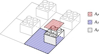
, is the ratio between the plan area and the unit wall-parallel area, as highlighted in figure 1. It is important to highlight that this roughness characterisation is far from universal (i.e. valid for any rough wall). As it is not the intention of the authors to investigate the latter, previous studies are followed to facilitate comparisons and highlight some of the limitations of this formulation. In the current study, the roughness is classified via three parameters:
 ${\it\lambda}_{F}$
,
 ${\it\lambda}_{P}$
and
 $h/{\it\delta}$
, where
 $h$
is the roughness height and
 ${\it\delta}$
is the boundary layer thickness.
Definition of the frontal and plan solidities. Black lines identify a single repeated unit and grey lines show how adjacent units are linked together to build the wall morphology. Inspired by Grimmond & Oke (Reference Grimmond and Oke1999).

Various studies have examined the effect of surface morphology on drag, and attempted to find correlations for
 $y_{0}=f({\it\lambda}_{F},{\it\lambda}_{P})$
. These studies have mainly classified the flow into two regimes: sparse (
 ${\it\lambda}_{F}<0.15$
), in which
 $y_{0}$
increases with solidity, and dense (
 ${\it\lambda}_{F}\geqslant 0.15$
), in which
 $y_{0}$
decreases. This is because as the density increases so does the roughness of the system, but a point comes where adding new elements merely serves to reduce the effective drag of those already present due to mutual sheltering; that is, they start to smoothen the roughness of the system (Grimmond & Oke Reference Grimmond and Oke1999). Comprehensive reviews of different morphometric drag prediction algorithms and an analysis of their accuracy can be found in Macdonald (Reference Macdonald1998) and Grimmond & Oke (Reference Grimmond and Oke1999) and more recently in Millward-Hopkins et al. (Reference Millward-Hopkins, Tomlin, Ma, Ingham and Pourkashanian2011) and Kanda et al. (Reference Kanda, Inagaki, Miyamoto, Gryschka and Raasch2013). The main limitation of these abovementioned studies is the fact that the suggested correlations
 $y_{0}=y_{0}({\it\lambda}_{F},{\it\lambda}_{P})$
are calculated over a collection of data sets from disparate sources with significantly different boundary conditions and characterised by geometrically different roughness elements. Regardless, among the morphometric bulk drag prediction methods, Macdonald’s (Reference Macdonald1998) method appears to be most widely used as it incorporates a broader range of scenarios when compared with other methods (Grimmond & Oke Reference Grimmond and Oke1999; Millward-Hopkins et al.
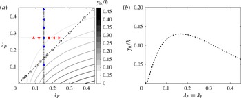
Reference Millward-Hopkins, Tomlin, Ma, Ingham and Pourkashanian2011). Figure 2(a) shows its prediction for
 $y_{0}$
as a function of
 ${\it\lambda}_{F}$
and
 ${\it\lambda}_{P}$
. Figure 2(b) shows the well-established empirical relationship between drag and
 ${\it\lambda}_{F}$
. This has been observed in previous studies on rough-wall boundary layers as reported by Grimmond & Oke (Reference Grimmond and Oke1999) and Jimenez (Reference Jimenez2004). However, the effect of plan solidity on bulk quantities is not clear. Additionally, effects of large roughness elements on these correlations remain unresolved. Castro (Reference Castro2007) pointed out that, although there is a substantial literature on rough-wall flows and there have been a number of attempts to develop useful correlations relating the surface friction to boundary layer parameters over a wide range of surface roughness, such correlations have mainly considered only small values of
 $h/{\it\delta}$
and it is not known how adequate they are at larger values of
 $h/{\it\delta}$
or what the critical value of
 $h/{\it\delta}$
should be.
(a) Contour plot of Macdonald’s prediction of the normalised roughness length behaviour as a function of
 ${\it\lambda}_{F}$
and
 ${\it\lambda}_{P}$
calculated using the expressions presented in Macdonald (Reference Macdonald1998) with
 $Cd=1.2$
,
 $k=0.41$
,
 ${\it\beta}=1$
and
 $A=4.43$
. The colourbar shows
 $y_{0}/h$
, the dashed line represents
 ${\it\lambda}_{F}\equiv {\it\lambda}_{P}$
(cubes), the dot-dashed line represents variation of
 ${\it\lambda}_{P}$
at fixed
 ${\it\lambda}_{F}$
and the dotted line stands for variation of
 ${\it\lambda}_{F}$
at fixed
 ${\it\lambda}_{P}$
. The filled symbols indicate the current experiment while the empty symbols indicate respectively ○ Kanda, Moriwaki & Kasamatsu (Reference Kanda, Moriwaki and Kasamatsu2004), ♢ Hagishima et al. (Reference Hagishima, Tanimoto, Nagayama and Meno2009) and ▫ Leonardi & Castro (Reference Leonardi and Castro2010). A cut along the dashed line in (a) is presented in (b).

Most previous studies that systematically explored the effect of surface morphology on drag were carried out with cubical roughness elements. These studies include both numerical and physical experiments (Cheng & Castro Reference Cheng and Castro2002b
; Coceal & Belcher Reference Coceal and Belcher2004; Kanda et al.
Reference Kanda, Moriwaki and Kasamatsu2004; Cheng et al.
Reference Cheng, Hayden, Robins and Castro2007; Santiago et al.
Reference Santiago, Coceal, Martilli and Belcher2008; Hagishima et al.
Reference Hagishima, Tanimoto, Nagayama and Meno2009; Leonardi & Castro Reference Leonardi and Castro2010, among various others). The open symbols in figure 2(a) show the cases examined in these studies. Any conclusion regarding the relationship between plan solidity and drag deduced from these studies is limited, since for cube roughness,
 ${\it\lambda}_{F}$
is equal to
 ${\it\lambda}_{P}$
. Similarly, any study on regular geometric staggered arrays of roughness for which the frontal and plan solidities are related by a mathematical relation (provided that there is no mutual sheltering between the elements) will lie on a similar curve to the dashed line in figure 2(a), although with a different slope. This means that the isolated effect of one of these two parameters will remain undetected. Isolation of the effects of the two solidities is only possible by following the dotted line and the dot-dashed line (or any alternative lines parallel to these lines), i.e. by varying
 ${\it\lambda}_{F}$
at a fixed
 ${\it\lambda}_{P}$
and vice versa. These branches have not been explored before. In this study, we explore the behaviour of drag along the dotted and dot-dashed lines in figure 2(a) in turbulent boundary layers with relatively large roughness elements (
 $h/{\it\delta}\approx$
0.1).
The aim of this study is to examine the individual effects of frontal and plan solidities at a constant
 $h/{\it\delta}\approx 0.1$
on the drag and the roughness sublayer. In order to do so, a systematic series of experiments was carried out by varying
 ${\it\lambda}_{F}$
at a fixed
 ${\it\lambda}_{P}$
and vice versa. A total of twelve different configurations were tested, and the resulting data, which cover the entire regime of solidities (sparse to dense), will be used to examine the drag generated by the different surfaces as well as their effect on the roughness sublayer. This will enable us to not only isolate the effects of
 ${\it\lambda}_{P}$
and
 ${\it\lambda}_{F}$
on the drag but also to examine the spatial similarity of the flow in the case of strong roughness (
 $h/{\it\delta}\approx 0.1$
).
2. Experimental facility and details
2.1. Experimental facility
The experiments were carried out in a suction wind tunnel at the University of Southampton. The same facility has been used for previous rough-wall studies such as those of Reynolds & Castro (Reference Reynolds and Castro2008) and Amir & Castro (Reference Amir and Castro2011). The tunnel has a working section of
 $4.5$
m in length, with a
 $0.9~\text{m}\times 0.6$
m cross-section. The free-stream turbulence intensity in the tunnel has been verified through hot-wire anemometry measurements to be homogenous across the cross-section and less than
 $0.3\,\%$
. In this study, (
 $x$
,
 $y$
,
 $z$
) are the streamwise, wall-normal and spanwise directions respectively, with the plane
 $y=0$
being the bottom surface of the baseboard onto which the roughness elements were located, as shown in figure 3(a). The mean and fluctuating velocities along these three directions are denoted as
 $(U,V,W)$
and
 $(u,v,w)$
respectively. The point statistics presented in this paper are obtained by ensemble averaging over a number of particle image velocimetry (PIV) realisations followed by spatial averaging across the PIV field of view (FOV). Experiments were conducted in nominally zero pressure gradient (ZPG) as the acceleration parameter (
 $K=({\it\nu}/U_{e}^{2})[\text{d}U_{e}/\text{d}x]$
, where
 ${\it\nu}$
is the air kinematic viscosity and
 $U_{e}$
is the velocity at the edge of the boundary layer) was less than
 $5\times 10^{-8}$
.
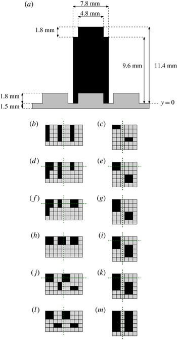
(a) LEGO® brick geometry. (b,d,f,h,j,l) Roughness element patterns with varying
 ${\it\lambda}_{F}$
at
 ${\it\lambda}_{P}=\text{const.}=0.27$
: (b) LF1,
 ${\it\lambda}_{F}=0.09$
; (d) LF2,
 ${\it\lambda}_{F}=0.12$
; (f) LF3,
 ${\it\lambda}_{F}=0.15$
; (h) LF4,
 ${\it\lambda}_{F}=0.18$
; (j) LF5,
 ${\it\lambda}_{F}=0.21$
; (l) LF6,
 ${\it\lambda}_{F}=0.24$
. (c,e,g,i,k,m) Roughness element patterns with varying
 ${\it\lambda}_{P}$
at
 ${\it\lambda}_{F}=\text{const.}=0.15$
: (c) LP1,
 ${\it\lambda}_{P}=0.11$
; (e) LP2,
 ${\it\lambda}_{P}=0.22$
; (g) LP3,
 ${\it\lambda}_{P}=0.27$
; (i) LP4,
 ${\it\lambda}_{P}=0.33$
; (k) LP5,
 ${\it\lambda}_{P}=0.39$
; (m) LP6,
 ${\it\lambda}_{P}=0.44$
. The dashed and dash-dotted lines in (b–m) indicate the position of the laser sheet during the measurements with respect to each repeated unit for the 2D and 3D PIV set-ups respectively. Dimensions are not in scale for ease of readability. Flow is from top to bottom in (b–m).

2.2. Roughness morphology
For rough surfaces, this study used LEGO® baseboards onto which LEGO® bricks (or blocks) were distributed in different patterns. Twelve different patterns were adopted in order to systematically examine the individual effects of frontal and plan solidities on the structure of the turbulence. Although not shown here for brevity, the effect of the incoming boundary layer (due to the baseboard) was quantified. This was found to be negligible as the flow was in equilibrium and fully developed over the bricks at the measurement location. Figure 3 shows the geometry of a LEGO® element and the basic repetitive units adopted to generate the different patterns analysed (frontal and plan solidity variations in figure 3(b,d,f,h,j,l) and (c,e,g,i,k,m) respectively). A single dark square in the top view is a single LEGO® brick. This brick has
 $\text{streamwise}\times \text{spanwise}$
dimensions of
 $7.8~\text{mm}\times 7.8~\text{mm}$
and its height is
 $h=11.4~\text{mm}$
(which includes the pin at the top), as shown in figure 3(a). Patterns LF1–LF6 represent cases for which the frontal solidity is varied at a fixed plan solidity, while in cases LP1–LP6 the plan solidity is varied at fixed frontal solidity. These variations follow the dotted and dot-dashed lines in figure 2(a). The different cases were designed on the basis of previous studies that show the locations of the peaks in
 $y_{0}$
at
 ${\it\lambda}_{P}=0.27$
and
 ${\it\lambda}_{F}=0.15$
(Grimmond & Oke Reference Grimmond and Oke1999; Jimenez Reference Jimenez2004). Progressive repositioning of the downstream roughness elements in the sheltered regions of the upstream obstacles allowed us to achieve variations in plan solidity at fixed frontal solidity. The same sheltering principle was applied to obtain the cases with varying
 ${\it\lambda}_{F}$
at fixed
 ${\it\lambda}_{P}$
. This enabled examination of the behaviour of the bulk quantities along the dotted and dot-dashed lines in figure 2(a). The filled symbols in figure 2(a) indicate the cases studied in this paper. The unit wall-parallel area of each repetitive unit was also kept fixed at
 $70.2~\text{mm}\times 39~\text{mm}$
and
 $46.8~\text{mm}\times 46.8~\text{mm}$
for the frontal and plan variation cases respectively. In evaluating
 ${\it\lambda}_{F}$
and
 ${\it\lambda}_{P}$
, the complete LEGO® bricks were considered (including the pins on top of the blocks, as shown in figure 1).
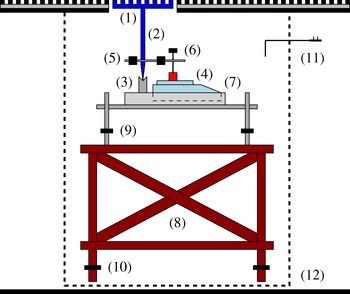
Schematic of the floating-element drag balance. Components: (1) measurement patch, (2) two-arm lever system, (3) knife edge, (4) precision scale, (5) counterbalance weights, (6) load-transfer adjustment pin, (7) H-frame containing the scale, (8) base structure, (9) fine adjustment feet, (10) rough adjustment feet, (11) Pitot tube, (12) sealed box.

2.3. Floating-element drag balance
The drag generated by the different wall morphologies was directly measured via a floating-element balance (which was based on the design of Krogstad & Efros Reference Krogstad and Efros2010). This balance was placed approximately
 $4~\text{m}$
downstream along the test section (the flow developed initially over the baseboard for 1.7 m and a further 2.3 m over the bricks). Figure 4 shows a schematic of the balance. A measurement patch (replica of the testing surface) was positioned in the tunnel floor through a cut hole; this element was mechanically connected to a two-arm lever system which converted the horizontal stress acting at the wall into a wall-normal load. A
 $370~\text{mm}\times 370~\text{mm}$
patch of the roughness was mounted on the top of the vertical arm of the balance to act as the sensing element. The measuring element was centred in a hole cut at the bottom of the wind tunnel floor surrounded by an approximately
 $1.5~\text{mm}$
gap to allow movement (i.e. readings onto the scale). It was important to prevent any possible airflow through this gap around the tile, as this would affect the measurements. As the present work was carried out in a suction wind tunnel, the static pressure inside the tunnel was always significantly lower than the atmospheric pressure. This necessitated mounting the entire balance in a sealed box, so that the measured force was not influenced. The sealed box was made out of soft plastic sheet. The static pressure inside both the tunnel and the box was monitored to prevent any pressure difference effect. This was found to be negligible within the measurement uncertainty. The relatively large sensing element size, compared with the original version in Krogstad & Efros (Reference Krogstad and Efros2010), allowed a number of repeated units to be included in the measurement patch. The lever system, which rested on a knife edge, allowed mechanical amplification of the forces based on the mutual length of the arms. The normal load was then measured by a high-sensitivity off-the-shelf precision Ohaus scale with a sensitivity of
 $0.01~\text{g}$
(gold series no. TAJ602/A). The measurement resolution, in the worst case, was typically
 $2.5\times 10^{-4}$
of the applied load. For additional details on the balance, the reader is referred to the original design in Krogstad & Efros (Reference Krogstad and Efros2010) and Efros (Reference Efros2011).
2.4. Particle image velocimetry
2.4.1. Planar PIV
Particle image velocimetry measurements were taken for all patterns at a free-stream velocity,
 $U_{\infty }$
, of 11.5 m s
 $^{-1}$
. The test location was at the same streamwise location as the skin-friction measurements. As will be shown later, at this free-stream velocity the flow over all surfaces is considered to meet fully rough conditions (or to be very close to this condition) to within the uncertainty of the skin-friction measurements. The flow was seeded with vaporised glycol–water solution particles (
 $1~{\rm\mu}$
m in diameter) illuminated with a
 $0.7~\text{mm}$
thick laser sheet produced by a pulsed New Wave Nd:YAG laser system operating at
 $200~\text{mJ}$
. The position of the laser sheet with respect to the roughness configuration is indicated by dashed lines in figure 3(b–m). Streamwise wall-normal
 $(x,y)$
planes were acquired at the spanwise centreline of the test section by a 16 megapixel high-resolution camera equipped with a Nikon
 $105~\text{mm}$
 $f/8$
lens at a fixed sampling frequency of 0.8 Hz. This was so that statistically uncorrelated measurements were acquired for each image pair. For each run, 2000 image pairs were acquired and processed with DaVis 8.0 software. The set-up allowed an FOV of
 $200~\text{mm}\times 136~\text{mm}$
(approximately
 $1.8{\it\delta}\times 1.3{\it\delta}$
streamwise–wall normal for each roughness configuration). Velocity vectors were obtained using
 $16~\text{pixel}\times 16~\text{pixel}$
final interrogation windows with
 $50\,\%$
overlap. The resulting spatial resolution was approximately
 $0.7~\text{mm}\times 0.7~\text{mm}$
for all cases and successive vectors were spaced at half that distance (due to the 50 % overlap). Images were preprocessed with averaged minimum intensity background subtraction. After this procedure, a field of 97–99 % good vectors was achieved, minimising the need for interpolation (when necessary a local mean interpolation was used).
The time delay between laser pulses across all of the cases was chosen such that the pixel displacement in the free stream was approximately 15 pixels. This ensured that the bias error of the PIV velocity measurements was less than 1 % of the full-scale velocity (given that the sub-pixel determination is estimated to have an uncertainty of approximately
 $\pm$
0.1 pixels – see Adrian & Westerweel Reference Adrian and Westerweel2011). The overall uncertainty in turbulence quantities was determined following Benedict & Gould (Reference Benedict and Gould1996) and was found to be less than
 $1\,\%$
in the mean velocity,
 $5\,\%$
and
 $8\,\%$
for the streamwise and normal turbulence intensities and
 $10\,\%$
for the shear stresses. These values are also in line with previous PIV-based studies on rough-wall turbulent flows (e.g. Wu & Christensen Reference Wu and Christensen2007).
The resolution of the current 2D data sets ranges between 28 and 42 wall units, due to differences in the skin-friction velocities generated by the different surface morphologies. The different local resolutions have a tangible effect on the turbulence statistics, in particular on the higher-order quantities. Therefore, for all the 2D PIV results presented herein, the data sets have been filtered with a low-pass Gaussian filter designed to match the local resolution at
 $l_{2D}^{+}=45$
. It must be noted that this filtered spatial resolution is comparable to (if not better than) previous cross-wire and PIV-based measurements presented in the literature.
2.4.2. Stereoscopic PIV
Given the high relative roughness height (
 $h/{\it\delta}$
), spanwise flow heterogeneity is to be expected within the roughness sublayer. To investigate this, stereoscopic PIV measurements were also carried out in the wall-normal–spanwise
 $(y,z)$
plane at roughly the same location as the 2D measurements. Two cameras with the same specifications as for the 2D measurements were used to acquire 1500 digital image pairs. An FOV covering a minimum of two spanwise repeated units (
 $1.5{\it\delta}\times 1.5{\it\delta}$
spanwise–wall normal) was resolved. A 1.5 mm thick laser sheet was used to illuminate the particles, and the time delay between the laser pulses (
 ${\rm\Delta}t=20~{\rm\mu}$
s) had to be reduced accordingly so that the particles would not leave the laser sheet plane. This reduced
 ${\rm\Delta}t$
had an influence on the averaged pixel displacement of the particles, and hence the PIV uncertainty. Measurements were carried out only across six cases, LF2, LF3, LF5 and LP2, LP4, LP5, as these represent conditions for sparse, medium and dense solidity regimes. The cameras were oriented at an angle of approximately
 $25^{\circ }$
to the measurement plane axis, which is appropriate to accurately resolve the out-of-plane velocity component (Raffel, Willert & Kompenhans Reference Raffel, Willert and Kompenhans1998). Scheimpflug adaptors were mounted on the lenses to help to maintain focus across the entire FOV by orienting the lens plane at an angle to the image plane, as discussed in Raffel et al. (Reference Raffel, Willert and Kompenhans1998). A two-plane calibration target was used for calibration, and self-calibration using Davis 8.0 was applied to improve the quality of the final velocity field (typically up to 2 pixel correction was used). Velocity vectors were obtained using
 $32~\text{pixel}\times 32~\text{pixel}$
final interrogation windows with
 $50\,\%$
overlap. This resolution was coarser than for the planar PIV measurements; however, given the nature of the measurements (i.e. flow perpendicular to the laser sheet) and the thickness of the laser sheet, this interrogation window was deemed sufficient. The worst-case resolution (
 $l_{3D}^{+}$
) across the different cases was approximately 120 wall units; therefore, for the same reasons as previously discussed, the 3D data set was filtered to match the local resolution across cases at
 $l_{3D}^{+}=125$
. This is comparable to similar measurements in the literature.
2.5. Indirect estimate of skin friction
The skin-friction velocity,
 $U_{{\it\tau}}=\sqrt{{\it\tau}_{w}/{\it\rho}}$
, where
 ${\it\tau}_{w}$
is the wall total shear stress and
 ${\it\rho}$
is the density of the fluid, is commonly assumed to be the average Reynolds shear stress in the log region. In this paper, we refer to this as an indirect method for determining the skin-friction velocity. Cheng & Castro (Reference Cheng and Castro2002b
) in their experiments on different urban roughnesses (all with
 ${\it\lambda}_{F}\equiv {\it\lambda}_{P}=0.25$
) demonstrated that an optimum estimation for the skin-friction velocity can be obtained from the spatially averaged Reynolds shear stress within both the roughness sublayer (RSL) and the inertial sublayer (ISL). The reader is referred to § 3.2 for further details on these regions. This shows that by spatially averaging over a roughness repeating unit, the logarithmic region can be extended to the roughness sublayer. In our investigation, the average across the streamwise direction and over a single repetitive unit yielded, within experimental uncertainty, the same results. Furthermore, Cheng et al. (Reference Cheng, Hayden, Robins and Castro2007) also argued that for boundary layer flows over staggered arrays of cubical elements, the
 ${\it\rho}\overline{uv}$
underestimates the surface stress by some 25 %. Therefore, a corrected estimate should be used, defined as (Reynolds & Castro Reference Reynolds and Castro2008)
 $$\begin{eqnarray}U_{{\it\tau}}=1.12\sqrt{-\overline{uv}}|_{2<y/h<3},\end{eqnarray}$$
where the Reynolds shear stress is evaluated from the plateau region in the roughness sublayer (as in Flack, Schultz & Shapiro Reference Flack, Schultz and Shapiro2005 and Castro Reference Castro2007). Both of these abovementioned approaches yield
 $U_{{\it\tau}}$
values that are within 5 % of each other. These values are also similar to the
 $U_{{\it\tau}}$
obtained by assuming it to be the maximum of the Reynolds shear stresses as in other studies in the literature (Manes, Poggi & Ridolfi Reference Manes, Poggi and Ridolfi2011).
2.6. Determination of aerodynamic parameters
Once the skin-friction velocity was known (as measured via the drag balance), a least-square-fit procedure was adopted to evaluate the zero-plane displacement,
 $d$
, and the roughness length,
 $y_{0}$
. This procedure was applied on the mean velocity field that was obtained by first ensemble averaging the data followed by streamwise averaging across the entire FOV. The log layer was assumed to exist for
 $1.5h\leqslant y\leqslant 0.2{\it\delta}$
as in Schultz & Flack (Reference Schultz and Flack2005). The fitting procedures were carried out with
 ${\it\kappa}=0.38$
for all surfaces. This value is close to the value of
 ${\it\kappa}$
suggested by Marusic et al. (Reference Marusic, Monty, Hultmark and Smits2013) for high-Reynolds-number smooth-wall boundary layers, where
 ${\it\kappa}=0.39\pm 0.02$
. A different choice of
 ${\it\kappa}$
alters the numerical values of
 $y_{0}$
and
 $d$
but not the trends shown in the following sections. It is important to highlight that, although it is common practice, to fit velocity profiles to determine the unknowns in (1.1), it bears great uncertainty. This is due to the difficulties, particularly at large
 $h/{\it\delta}$
, in determining both the skin-friction velocity and the log-law boundaries (Acharya, Bornstein & Escudier Reference Acharya, Bornstein and Escudier1986; Castro Reference Castro2007; Segalini, Örlü & Alfredsson Reference Segalini, Örlü and Alfredsson2013). The reduction of the wall-normal range of the logarithmic layer due to the increasing importance of the RSL is another important factor to take into account.
3. Results and discussion
Section 3.1 shows the effect of the surface morphology on the aerodynamic parameters. Section 3.2 examines the effect of the wall morphology on the RSL. Finally, § 3.3 introduces the details of the POD analysis and its implementation to examine the global spatial structure of the flow over different types of roughness. The turbulent kinetic energy content at different flow scales is also investigated.
3.1. Effect of surface morphology on aerodynamic parameters
Before examining the effect of the surface morphology on aerodynamic parameters, it is useful to determine whether these surfaces are fully rough, in order to ensure that the results presented herein are solely due to the different roughness morphologies, rather than the product of a change in Reynolds number (i.e. viscous effects). There is general consensus in the literature that fully rough conditions are attained when
 $y_{0}^{+}>2$
(Castro Reference Castro2007) to
 $h_{s}^{+}>70$
(Flack et al.
Reference Flack, Schultz and Shapiro2005). Here,
 $h_{s}$
is the equivalent sand-grain roughness as in Nikuradse (Reference Nikuradse1933). Recent findings have cast doubt on these limits and pointed out that, depending on the surface morphology, values up to
 $y_{0}^{+}>10$
might be necessary to guarantee fully rough conditions (Castro, Segalini & Alfredsson Reference Castro, Segalini and Alfredsson2013). In order to assess whether the surfaces in the current study are in the fully rough regime, the friction coefficient,
 $C_{f}=2(U_{{\it\tau}}/U_{\infty })^{2}$
, was measured with the drag balance at different inflow velocities and hence different Reynolds numbers (
 $Re_{h}=U_{\infty }h/{\it\nu}$
). A velocity range between
 $11.5$
and
 $20$
m s
 $^{-1}$
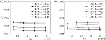
was considered and the results are presented in figure 5(a,b) for the frontal and plan solidity cases respectively. It is clear that the variation in the measured friction coefficient at different velocities is within the limits of uncertainty. It follows that, within the measurement uncertainty, all cases in both
 ${\it\lambda}_{F}$
and
 ${\it\lambda}_{P}$
are considered to be in the fully rough regime, i.e. Reynolds number independent. Hence, if differences are observed in the aerodynamic parameters, these are purely an effect of surface morphology. It should be pointed out that additional velocities were tested (down to
 $6$
m s
 $^{-1}$
). These results are omitted here as the measurement resolution was lower than the presented cases. However, these clearly showed Reynolds number dependence of the skin friction (i.e. transitionally rough regimes). On increasing the Reynolds number, nevertheless,
 $C_{f}$
shows the plateaux described above, which is an indication that the ‘fully rough regime’ is reached.
Skin-friction coefficient,
 $C_{f}$
, as a function of Reynolds number, as a function of (a)
 ${\it\lambda}_{F}$
(
 ${\it\lambda}_{P}=\text{const.}=0.27$
) and (b)
 ${\it\lambda}_{P}$
(
 ${\it\lambda}_{F}=\text{const.}=0.15$
).

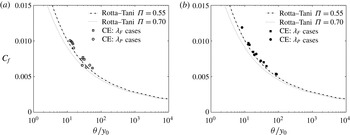
Variation of
 $C_{f}$
as a function of
 ${\it\theta}/y_{0}$
for (a) the Reynolds stress method (via fitting of (2.1)) and (b) the drag balance method (direct measurement). The dotted and dashed–dotted curves refer to the standard two-parameter family results with wake strengths of
 ${\it\Pi}=0.55$
and
 $0.7$
. The roughness length,
 $y_{0}$
, is calculated via a least-square-fit procedure for
 $1.5h<y<0.2{\it\delta}$
.

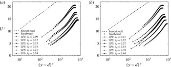
Mean velocity profiles in inner scales as a function of (a)
 ${\it\lambda}_{F}$
(
 ${\it\lambda}_{P}=\text{const.}=0.27$
) and (b)
 ${\it\lambda}_{P}$
(
 ${\it\lambda}_{F}=\text{const.}=0.15$
). The solid lines represent the real data resolution while markers are spaced every five vectors for clarity.

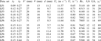
Relevant experimental parameters for frontal and plan solidity variations. The
 $U_{{\it\tau}}$
values reported are obtained via floating-element drag balance. These values of
 $U_{{\it\tau}}$
are used in all subsequent analyses. The aerodynamic parameters are calculated through a log-law fit with
 ${\it\kappa}=0.38$
in the range
 $1.5h\leqslant y\leqslant 0.2{\it\delta}$
. The
 $U_{e}$
values reported herein are from the PIV results.

The validity of the Reynolds stress method (via fitting of (2.1)) for the skin-friction determination can be established by comparing the results with the direct friction balance measurements. The value of
 $C_{f}$
as a function of the normalised momentum thickness,
 ${\it\theta}/y_{0}$
, is shown in figure 6. In particular, figure 6(a) shows results using the indirect method (via (2.1)) and figure 6(b) using the direct method (friction balance) for skin-friction estimation. This type of plot was first proposed by Castro (Reference Castro2007) and will allow us to estimate whether the current data agree with previous findings. Most of the results from rough-wall studies have been found to scatter around the two curves (for different values of the wake parameter
 ${\it\Pi}$
) shown in figure 6 (Castro Reference Castro2007). It can be seen that our data using both methods are consistent with previous results in the literature. The indirect measurements results (via (2.1)) compare well with the direct measurements (within
 $10\,\%$
) given the uncertainty in determination of the skin-friction velocity (Acharya et al.
Reference Acharya, Bornstein and Escudier1986) and the log-law boundaries used to determine the roughness length (Segalini et al.
Reference Segalini, Örlü and Alfredsson2013). The skin-friction values obtained via the floating-element drag balance are used in all of our analyses. Relevant boundary layer characteristics for all of the cases are given in table 1. It can be seen from the table that all cases have
 $y_{0}^{+}\geqslant 10$
and hence we conform to the revised estimates for fully rough conditions.
Figure 7(a) shows the mean velocity profiles in inner scales for the different cases of
 ${\it\lambda}_{F}$
at fixed
 ${\it\lambda}_{P}$
. It can be seen that, compared with a smooth-wall case ((1.1) with
 $d=0$
,
 $B=5$
and
 ${\rm\Delta}U^{+}=0$
), the roughness is responsible for a uniform downward shift of the log region, as expected. The plain baseboard case, referring to the wind tunnel floor being covered only with baseboard but no bricks, is also reported for comparison. It shows that the presence of the blocks (cases LF1–LF6) is indeed responsible for generating a further shift of the log-law compared with the baseboard case. Figure 7(b) shows the behaviour of the mean velocity profiles for the different
 ${\it\lambda}_{P}$
cases. Once again the roughness is responsible for a downward shift of the log-law region. According to Jimenez (Reference Jimenez2004), the log layer over a rough surface should remain intact only for
 $h/{\it\delta}<1/40$
, so that the velocity profiles should be self-similar in the other region. However, when
 $h/{\it\delta}>1/40$
, a situation similar to flows over obstacles is encountered and the universality of velocity statistics breaks down. A discussion on the critical relative roughness height,
 $h/{\it\delta}$
, for which Townsend’s similarity hypothesis fails is outside the scope of this study. However, it can be clearly observed in figure 7 that a log-law seems to be well defined for all velocity profiles. This is not unique given that previous studies (Castro Reference Castro2007; Amir & Castro Reference Amir and Castro2011, among others) have shown that some rough walls conform to outer-layer similarity up to
 $h/{\it\delta}\approx 0.2$
, which is even more severe than the morphologies presented herein. It is therefore anticipated that Jimenez’s criterion is unnecessarily restrictive, given that these surfaces show mean velocity similarity.
To further quantify the effect of the surface morphology on the bulk drag, the roughness function can be calculated. Figure 8 shows the normalised roughness length,
 $y_{0}/h$
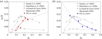
, as a function of both solidities. It is shown in figures 8(a) and 8(b) that the behaviour of the roughness length as a function of frontal and plan solidity is drastically different. Figure 8(a) shows that the roughness length (which is related to the total drag) increases in the sparse regime, and indicates a marginal decrease after the peak for increased values of frontal solidity, as in Leonardi et al. (Reference Leonardi, Orlandi, Smalley, Djenidi and Antonia2003) and Leonardi & Castro (Reference Leonardi and Castro2010). Within the range of solidity explored herein, the bulk drag seems to reach a peak at
 ${\it\lambda}_{F}=0.21$
for a fixed
 ${\it\lambda}_{P}=0.27$
. The roughness length results, in figure 8(a), closely follow the skin-friction trends as a function of both the solidities, as shown in table 1. The drag peak location herein is partially in contrast with previous studies, for which it was found at
 ${\it\lambda}_{P}\equiv {\it\lambda}_{F}\approx 0.15$
(Kanda et al.
Reference Kanda, Moriwaki and Kasamatsu2004; Hagishima et al.
Reference Hagishima, Tanimoto, Nagayama and Meno2009; Leonardi & Castro Reference Leonardi and Castro2010) and
 ${\it\lambda}_{P}\equiv {\it\lambda}_{F}\approx 0.16$
(Coceal & Belcher Reference Coceal and Belcher2004; Santiago et al.
Reference Santiago, Coceal, Martilli and Belcher2008). These differences are perhaps not surprising giving the high uncertainty in the fitting procedure which results in the visible scatter of the data for different studies in figure 8(a), even when values of similar frontal and plan solidity are considered. This scatter could also be partly due to the fact that prescribing a set of
 ${\it\lambda}_{F}$
and
 ${\it\lambda}_{P}$
values results in a non-unique mapping of a roughness geometry – i.e. different geometries can generate the same combination of solidities. Furthermore all of the previous studies used cubical elements, for which
 ${\it\lambda}_{F}\equiv {\it\lambda}_{P}$
, while in the current experiment the plan solidity has been kept constant. Additionally, the comparable studies also have different
 $h/{\it\delta}$
values. Finally, given that the current data set is a collection of discrete points, the reported peak at
 ${\it\lambda}_{F}=0.21$
only implies that the effective peak value should be located somewhere in the range
 ${\it\lambda}_{F}=0.18$
–0.24, which is consistent with previous findings. It is important to note that this result only applies within
 $0.11\leqslant {\it\lambda}_{F}\leqslant 0.27$
, as no information is available outside this range.
It must be highlighted that the existence of this peak in the bulk drag is not necessarily in agreement with Macdonald’s prediction, which prescribes a monotonic increase of the drag as the frontal density of the elements increases. Given the scatter in data, it is difficult to interpret this further. However, as emphasised previously, in the current experiment the influences of frontal and plan solidity have been decoupled by keeping one of the two parameters fixed at a time, and the trend does suggest a peak in drag for
 ${\it\lambda}_{F}$
at a given
 ${\it\lambda}_{P}$
. The behaviour of the bulk drag with plan solidity is shown in figure 8(b), and it reveals a completely different feature. The roughness length is found to monotonically decrease as the plan density increases. It is not possible to compare this behaviour with previous studies for which
 ${\it\lambda}_{F}\equiv {\it\lambda}_{P}$
, since in that case changes in one solidity parameter result in modifying the other one.
Normalised roughness length,
 $y_{0}/h$
, as a function of (a)
 ${\it\lambda}_{F}$
and (b)
 ${\it\lambda}_{P}$
. Current experiment (CE) refers to values obtained by a log-law least-square fit in the range
 $1.5h<y<0.2{\it\delta}$
.

It is expected that the roughness length should increase as the frontal density of the elements increases, reaching a peak beyond which it should decrease, for further increase in roughness density. This expected behaviour is verified in the case of frontal density variation, which shows a peak for
 ${\it\lambda}_{F}=0.21$
. An increase in frontal solidity (cases LF1–LF6) increases the frontal blockage, reducing the free space available for the flow, forcing it up and over the elements, and hence resulting in a drag increase. However, for plan solidity cases, the bulk drag monotonically decreases with increasing
 ${\it\lambda}_{P}$
. This could be due to the fact that progressive increase of the plan area at fixed
 ${\it\lambda}_{F}$
, and hence at fixed unit wall-parallel area (as in cases LP1–LP6), results in a transition from ‘k-type’ to ‘d-type’ roughness. This progressive transition results in a decrease in drag with increasing plan solidity. It must be noted that we use the ‘k-type’ and ‘d-type’ terms only to relate to the flow mechanisms that are shown to be associated with these classifications and not to the type of roughness. The flow behaviour between the roughness elements, following Grimmond & Oke (Reference Grimmond and Oke1999), depends upon the ratio between the roughness height,
 $h$
, and the average streamwise spacing between elements,
 $W_{c}$
(the width of the channel between subsequent elements). An ‘isolated flow regime’ is expected when
 $h/W_{c}<0.3$
, a ‘wake interference regime’ for
 $0.3<h/W_{c}<0.65$
and a ‘skimming flow regime’ for
 $h/W_{c}>0.65$
. It is easy to verify from figure 3(b–m) that, while the average spacing is almost constant for the
 ${\it\lambda}_{F}$
variation, the same is not true for the
 ${\it\lambda}_{P}$
cases. In the latter, in fact, this spacing decreases from case LP1 to LP6. This is because of the necessity to keep the unit wall-parallel area fixed, enforcing changes in plan solidity at fixed
 ${\it\lambda}_{F}$
. Therefore, this results in cases LF1–LF6 all belonging to the ‘wake interference regime’ (
 $h/W_{c}\approx 0.39$
), while a transition between the ‘isolated flow regime’ and the ‘skimming regime’ is to be expected between cases LP1 and LP6 (
 $h/W_{c}$
ranging between 0.27 and 0.55).
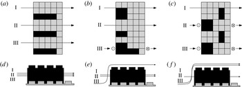
Field patterns and associated flow regimes for different elements for increasing
 ${\it\lambda}_{F}$
: LF1 (a,d), LF3 (b,e) and LF5 (c,f). The
 $\odot$
symbols stand for arrows pointing towards the reader and symbolise path lines of particles that deviate upward; the
 $\otimes$
symbols stand for path lines of particles that deviate downward. Flow is from left to right.

It is certainly possible under some circumstances that an increase in frontal blockage can be in competition with the transition from ‘k-type’ to ‘d-type’ (i.e. changes in
 $h/W_{c}$
). In those cases, the bulk drag of different surfaces with different
 ${\it\lambda}_{F}$
and
 ${\it\lambda}_{P}$
can be a constant. Alternately, depending on the pattern of the repeating unit, the drag could even decrease with increasing
 ${\it\lambda}_{P}$
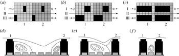
. Sketches that describe the scenarios discussed above are shown in figures 9 and 10 respectively. Figure 9(a–c) shows a progressive increase of the spanwise blockage in the flow. This results in the flow rising upward towards the top of the elements and over them (i.e. ‘k-type’) resulting in an increase in bulk drag. Figure 10(d–f) shows a representation of the transition mechanism, with elements in subsequent repeated units becoming closer to each other, resulting in the formation of stable vortices in the grooves between the elements. This ensures that the eddy shedding from the elements into the flow is progressively more negligible. These stable recirculation vortices are effectively isolating the elements from the flow (i.e. ‘d-type’), which rides almost undisturbed over the elements resulting in a reduction of the generated drag.
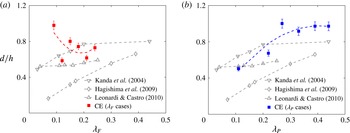
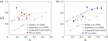
In addition to the roughness length, the values of the zero-plane displacement,
 $d$
, as a function of the frontal and plan solidities have also been calculated and are shown in figures 11(a) and 11(b) for frontal and plan solidities respectively. Since a value of
 $d>h$
would be physically meaningless (Jackson Reference Jackson1976), these values are forced to be
 $d=h$
as in Iyengar & Farell (Reference Iyengar and Farell2001). It is clearly visible in figure 11(b) that the virtual origin increases with an increase in plan solidity until it approaches its asymptote at
 $d=h$
. The latter is qualitatively consistent with previous studies which have shown that the zero-plane displacement tends to assume larger values (i.e.
 $d$
tends to
 $h$
) as the plan solidity increases (Kanda et al.
Reference Kanda, Moriwaki and Kasamatsu2004; Hagishima et al.
Reference Hagishima, Tanimoto, Nagayama and Meno2009; Leonardi & Castro Reference Leonardi and Castro2010). This trend is also consistent with the predictions from Macdonald (Reference Macdonald1998). Although the quality of the fit deteriorates, an opposite trend seems to emerge in figure 11(a). For a frontal solidity variation, the virtual origin decreases as
 ${\it\lambda}_{F}$
increases. It must be noted that the trend followed by previous studies does not capture the conditions of the present experiments – the data were obtained over cube roughness and hence the behaviour with
 ${\it\lambda}_{F}$
is exactly the same as for
 ${\it\lambda}_{P}$
.
Field patterns and associated flow regimes for different elements for increasing
 ${\it\lambda}_{P}$
: LP1 (a,d), LP3 (b,e) and LP6 (c,f). The
 $\odot$
symbols stand for arrows pointing towards the reader and symbolise path lines of particles that deviate upward; the
 $\otimes$
symbols stand for path lines of particles that deviate downward. Flow is from left to right. The light and dark grey areas in (a–c) indicate repetitive units of subsequent elements.

Normalised zero-plane displacement,
 $d/h$
, as a function of (a)
 ${\it\lambda}_{F}$
and (b)
 ${\it\lambda}_{P}$
. Current experiment (CE) refers to values obtained by a log-law least-square fit in the range
 $1.5h<y<0.2{\it\delta}$
.
3.2. Effect of surface morphology on the roughness sublayer
Given the high relative roughness (
 $h/{\it\delta}\approx 0.1$
), flow heterogeneity along the spanwise direction is to be expected at least within the roughness sublayer. This region has usually been identified to extend up to five roughness heights (Cheng & Castro Reference Cheng and Castro2002a
; Flack, Schultz & Connelly Reference Flack, Schultz and Connelly2007). To investigate the flow heterogeneity, results from stereoscopic PIV measurements in the wall-normal–spanwise
 $(y,z)$
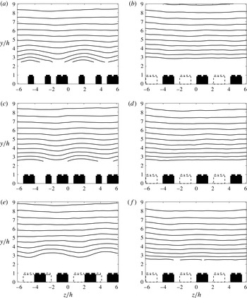
plane are presented. Contour plots of mean streamwise velocity are shown in figure 12 for both
 ${\it\lambda}_{F}$
and
 ${\it\lambda}_{P}$
cases in (a,c,e) and (b,d,f) respectively. The extent of the FOV has been cropped so that two to three entire repeated units are contained in the presented graphs, hence allowing the effect of the edges of a single unit to be taken into account. To facilitate the interpretation of the figures, the brick locations are also highlighted in the figure. Three/four bricks combined represent one repeated unit for the
 ${\it\lambda}_{F}$
cases, while only two bricks combine to form the
 ${\it\lambda}_{P}$
cases (as in figure 3
b–m), keeping the overall size of the FOV roughly the same. Full black bricks stand for elements in the measurement plane while dashed lines represent bricks out of the measurement plane, yet in the same repeated unit. For the frontal solidity cases (in figure 12
a,c,e), a mean-flow distortion due to the presence of the elements for low values of
 $y/h$
is clearly visible. This effect is much greater for the
 ${\it\lambda}_{F}$
cases than for the
 ${\it\lambda}_{P}$
cases (in figure 12
b,d,f). For all cases, the contour lines appear to be reasonably flat farther away from the crest of the roughness elements suggesting a localised effect of roughness. Moreover, very little differences in mean streamwise velocity across the span are found above
 $5h$
, which is therefore suggested to be the upper edge of the roughness sublayer.
Mean (ensemble-averaged) streamwise velocity contours,
 $U$
, in the
 $(y,z)$
plane for sparse (a,b), medium (c,d) and dense regimes (e,f) as a function of
 ${\it\lambda}_{F}$
(
 ${\it\lambda}_{P}=\text{const.}=0.27$
) in (a,c,e) and
 ${\it\lambda}_{P}$
(
 ${\it\lambda}_{F}=\text{const.}=0.15$
) in (b,d,f). The lowest contour level
 $U/U_{e}=0.5$
, with a contour spacing of 0.05. Bricks in the measurement plane are represented in full black, while bricks out of the measurement plane in the same repeated unit are identified by dashed lines. The mean flow is into the plane along the positive
 $x$
-axis.

There is very little information available in the literature on the definitions used to determine the depths of the ISL and the RSL, and this is the subject of ongoing debate (Cheng & Castro Reference Cheng and Castro2002a
,Reference Cheng and Castro
b
). However, there is some consensus on the necessity to look at the Reynolds shear stress characteristics. It is outside the scope of this paper to further investigate the best way to define these regions, and therefore definitions from previous literature are followed (Raupach, Antonia & Rajagopalan Reference Raupach, Antonia and Rajagopalan1991; Cheng & Castro Reference Cheng and Castro2002b
; Cheng et al.
Reference Cheng, Hayden, Robins and Castro2007). The upper boundary of the RSL is defined as the location where the spatially spanwise-averaged wall-normal profiles converge to within 10 %. Similarly, the ISL is defined as the region where the vertical variation of the shear stress may be neglected or its variation is within a certain threshold (i.e.
 ${<}5\,\%$
). Both of these regions are defined relative to the mean (ensemble) Reynolds shear stresses spatially averaged across the FOV.
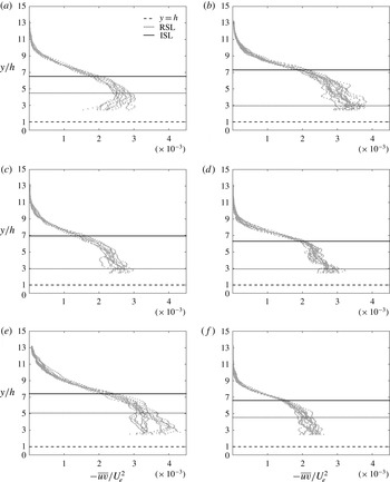
Figure 13 shows the extent of the abovementioned regions within the boundary layer for frontal and plan solidity variation in (a,c,e) and (b,d,f) respectively. Grey solid marks indicate profiles along the spanwise direction across the entire FOV, which includes more than one complete repeated unit. In all of these graphs, the roughness height is defined from the bottom of the baseboard (i.e. the actual wall
 $y=0$
). The height of the roughness elements is marked by a dashed black line and it is constant. For all cases, the extent of the RSL is found to be confined to
 ${\approx}5h$
, which is consistent with previous findings (Flack et al.
Reference Flack, Schultz and Connelly2007). Moreover, for the frontal solidity cases (a,c,e) the RSL depth seems to reach a minimum to then increase again as the
 ${\it\lambda}_{F}$
increases. Therefore, the extent of this region follows a reverse trend when compared with that of the roughness length (or bulk drag) behaviour (in figure 8
a). It seems that an increase in drag results in a decrease of the RSL depth and vice versa. This same trend is found for the plan solidity cases (b,d,f), where the extent of the RSL seems to increase with the solidity, while the drag was found to decrease (see figure 8
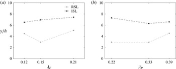
b). The abovementioned observations are summarised in figures 14(a) and 14(b), which show the variation of the RSL and ISL as a function of
 ${\it\lambda}_{F}$
and
 ${\it\lambda}_{P}$
respectively. It is important to note that differences can arise depending on the choice of threshold used to define the regions; however, the trend across all cases was found to be unaffected by the magnitude of the threshold.
Normalised Reynolds shear stress profiles,
 $-\overline{uv}/U_{e}^{2}$
, for sparse (a,b), medium (c,d) and dense regimes (e,f) as a function of
 ${\it\lambda}_{F}$
(
 ${\it\lambda}_{P}=\text{const.}=0.27$
) in (a,c,e) and
 ${\it\lambda}_{P}$
(
 ${\it\lambda}_{F}=\text{const.}=0.15$
) in (b,d,f). The grey solid symbols represent the shear stress data (only one in every five vectors is shown for clarity), the dashed black line shows
 $y=h$
(canopy layer), while the dotted and solid black lines represent the extents of the RSL and ISL respectively.

The RSL and ISL depths as a function of (a)
 ${\it\lambda}_{F}$
(
 ${\it\lambda}_{P}=\text{const.}=0.27$
) and (b)
 ${\it\lambda}_{P}$
(
 ${\it\lambda}_{F}=\text{const.}=0.15$
). Only available 3D data sets are presented.

It is worth noting that recent studies (Mejia-Alvarez & Christensen Reference Mejia-Alvarez and Christensen2013; Barros & Christensen Reference Barros and Christensen2014) have experimentally shown that mean-flow heterogeneities exist in the spanwise–wall-normal plane of rough-wall turbulent boundary layers, particularly over a complex roughness which exhibited large-scale streamwise-elongated patches of elevated height. This heterogeneity extended outside the RSL all the way to the free stream. This phenomenon is due to the presence of spanwise–wall-normal mean secondary flow in the form of mean streamwise vorticity associated with counter-rotating boundary-layer-scale circulations (Barros & Christensen Reference Barros and Christensen2014). The latter induces regions of high and low momentum (HMPs and LMPs respectively). Such patterns are also in agreement with the behaviour found by Reynolds et al. (Reference Reynolds, Hayden, Castro and Robins2007) for flow over regular cubical roughness. The mean-flow heterogeneities in both cases were here found to be in correspondence with the periodic spanwise roughness spacing. However, although some of the cases examined herein resemble Barros & Christensen (Reference Barros and Christensen2014)’s geometry (in particular case LP6), the current investigation found no trace of this heterogeneity in the free stream. This is in disagreement with the aforementioned studies and it is perhaps due to the fact that the spanwise spacing between elements in the cases examined in the current study is not significant enough to induce this characteristic behaviour. Further exploration of this aspect is outside the scope of this work.
3.3. Proper orthogonal decomposition
To explore the spatial characteristics and the behaviour of the flow and its dependence on wall morphology, a snapshot-based POD analysis was carried out (Berkooz, Holmes & Lumley Reference Berkooz, Holmes and Lumley1993). This technique generates a basis for modal decomposition of the ensemble of instantaneous fluctuating velocity fields and provides the most efficient way of identifying the motions which, on average, contain a majority of the turbulent kinetic energy (TKE) in the flow. The energy contribution of the singular value across the modes, hence its shape, depends on the local spatial resolution of the data set, as discussed in Pearson, Goulart & Ganapathisubramani (Reference Pearson, Goulart and Ganapathisubramani2013). This is because the energy content of each
 $i$
th mode depends on the smallest resolved scale in the flow (i.e. in the data set). The global resolution of the current 2D data set ranged between 30 and 40 wall units, due to differences in the skin-friction velocity generated by the different surface morphologies. This resulted in a variation of the Kármán number in the range of
 $Re_{{\it\tau}}\approx 4900$
–7500. For this reason, the current data set was filtered with a low-pass Gaussian filter designed to match the local resolution at
 $l_{2D}^{+}=45$
. Moreover, the FOV across the different cases was also matched to the region
 $-0.6{\it\delta}<x<0.6{\it\delta}$
in the streamwise and
 $1.5h\leqslant y\leqslant {\it\delta}$
in the wall-normal direction to allow for meaningful comparisons. The results presented herein were obtained by performing the POD calculation over the combined
 $(u,v)$
data.
The first four low-order POD modes for the LF2 case. The flow is from left to right in (a–d). The POD modes are calculated on the combined
 $(u,v)$
field.

The first four low-order POD modes for the LP2 case. The flow is from left to right in (a–d). The POD modes are calculated on the combined
 $(u,v)$
field.

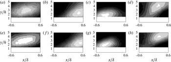
Figure 15 shows contour plots of the shapes of the first four energetic POD modes. These are specific to one case (i.e. LF2,
 ${\it\lambda}_{F}=0.09$
,
 ${\it\lambda}_{P}=0.27$
), although they were found to be consistent (and indistinguishable) in shape and order across all surface morphologies, regardless of the regime. For comparison, the first four modes for LP2 (
 ${\it\lambda}_{F}=0.15,{\it\lambda}_{P}=0.11$
) are shown in figure 16. The rest of the results are omitted for the sake of brevity. This similarity is remarkable considering the different patterns adopted to generate the morphologies (see figure 3
b–m) and is a testimony of some form of universality across rough walls. Regions of high and low streamwise momentum (or vice versa), which are highlighted in black and white respectively, are clearly visible in figure 15 (although the colourbar is arbitrary). The shape of the most energetic mode (mode 1) is characterised by an elongated large-scale high- (or low-) momentum region. Mode 2 embodies instead an inclined shear layer that separates a high-momentum region below it from a low-momentum region appearing above it (or vice versa since the sign of the values is arbitrary and will depend on the eigenvalue itself). A similar shape is assumed by mode 3 where the inclination of the shear layer is reversed compared with the flow direction. Mode 4 is dominated by three distinctive regions: two localised low-momentum regions are separated by an elongated forward-leaning streamwise high-momentum region. As Adrian, Christensen & Liu (Reference Adrian, Christensen and Liu2000) discussed, while POD modes are not representative of the actual coherent structures present in the flow, but more of the energy of those structures, they do provide a qualitative glimpse at the dominant flow field associated with each mode and its variability from one mode to another. A trend of increasingly smaller structures for higher modes is generally found throughout all cases. Therefore, the low-order modes tend to be associated with large-scale structure, while the higher-order modes are representative of increasingly smaller scales. Comparison of the first 10 modes across all of the morphologies shows identical mode shapes, indicating that there is a degree of structural similarity regardless of the roughness morphology (here omitted for brevity). Yet, the aerodynamic parameters are very different across the cases.
The differences in flow structure that perhaps lead to the differences in the aerodynamic parameters might not be evident when the structure of the entire boundary layer is examined using analysis of POD modes. It might be more meaningful to employ this analysis confined to the roughness sublayer so as to isolate any difference in the flow structures between the different roughness morphologies.
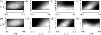
The first four low-order POD modes in the roughness sublayer for (a–d) the sparse and (e–h) the dense frontal solidity regime. The flow is from left to right in (a–h). The POD modes are calculated on the combined
 $(u,v)$
field. It should be noted that the aspect ratio of these figures has been changed to highlight the roughness sublayer. The wall-normal direction has been stretched compared with figures 15 and 16.

3.3.1. Effect of surface morphology of the structure of the RSL
To further investigate the effect of the surface morphology in the near-canopy (or near-wall) layer, the same POD analysis can be carried but this time only focusing on the roughness sublayer. As shown in the previous sections, this region appears to be where the roughness effect is confined. For this purpose, the POD analysis was carried out, as in the previous case, but the FOV was restricted to the roughness sublayer,
 $-0.6{\it\delta}<x<0.6{\it\delta}$
in the streamwise and
 $1.5h<y<5h$
in the wall-normal direction. The chosen vertical limit is based on the consensus in the literature as to the extent of the roughness sublayer (
 $y/h\approx 3$
–5 as in Flack et al.
Reference Flack, Schultz and Connelly2007). Figure 17 shows the result of this procedure for the frontal solidity cases. Figure 17(a–d) shows results for the sparse regime (i.e. LF2), while figure 17(e–h) shows similar plots in the dense regime (i.e. LF5). The mode shapes appear to be qualitatively the same in these ‘near-canopy’ fields; however, it must be highlighted that, for ease of readability, the
 $y$
-axis is ‘stretched’ compared with the previous cases in figures 15 and 16. The only difference between the two regimes (i.e. sparse versus dense) is that modes 3 and 4 switch their order between the sparse and dense regimes. Mode 4 in the sparse regime seems to correspond to mode 3 in the dense regime and vice versa. This suggests that the relative energy content in mode 3 compared with mode 4 is higher in one case and lower in the other. The mode number where this change in mode shape occurs is named the ‘cutoff’ mode and can be taken to represent the breakdown of the spatial similarity of the flow within the roughness sublayer. It should be noted that this breakdown was not present in the full-field modes, where the energy in the outer region seemingly dominates the energy contained in the roughness sublayer. Physically, this means that a redistribution of energy across scales has taken place; therefore, the energy-relevant scales are different in size/shape for the different regimes. An increase in frontal solidity results in redistributing the energy towards scales that are inclined to the wall (mode 3 compared with mode 4). A similar POD analysis for the plan solidity cases is shown in figure 18. It is noticeable that the mode shapes appear to be similar to the previously discussed full-field cases and that for this solidity variation the energy redistribution is absent. This suggests that there is a higher degree of spatial similarity in the energy-containing motions in the roughness sublayer across the different plan solidities.
These findings are consistent with the hypothesis presented in § 3.1. When the frontal solidity increases, the flow is progressively forced up and over the elements; hence a degradation of the local coherency is observed at high
 ${\it\lambda}_{F}$
values, introducing energy into scales that are inclined to the wall, which is revealed by the appearance of the ‘cutoff’ mode. This process is entirely absent for
 ${\it\lambda}_{P}$
variations, as the frontal blockage is fixed; hence the cutoff mode does not appear in the RSL as the flow over the canopy is not significantly altered.
The first four low-order POD modes in the roughness sublayer for (a–d) the sparse and (e–h) the dense plan solidity regime. The flow is from left to right in (a–h). The POD modes are calculated on the combined
 $(u,v)$
field. It should be noted that the aspect ratio of these figures has been changed to highlight the roughness sublayer. The wall-normal direction has been stretched compared with figures 15 and 16.

3.3.2. Effect of surface morphology on energy distribution across scales
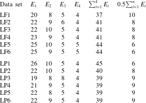
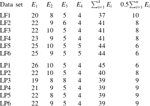
Table 2 shows the fractional turbulent kinetic energy (FTKE) contribution
 $E_{i}$
of the
 $i$
th POD mode,
 ${\it\phi}_{i}$
, to the total TKE for the
 ${\it\lambda}_{F}$
and
 ${\it\lambda}_{P}$
cases. It can be seen that cases with lower
 ${\it\lambda}_{F}$
tend to be characterised by lower energy content in the first POD mode. For example, mode 1 for the LF1 case contains only
 ${\approx}20\,\%$
of the total energy, while for the LF3 and LF6 cases, its content reaches
 ${\approx}22\,\%$
and
 ${\approx}25\,\%$
respectively. This seems to suggest that the effect of an increased frontal solidity would be to redistribute the energy towards the lowest-order POD modes and therefore the larger scales. It can also be inferred that the plan solidity cases present an opposite trend, where the first mode for the sparse case contains almost 26 % of the total TKE while the contributions of the same mode for the medium and dense regimes (LP4 and LP6 cases for example) are only 21 % and 22 % respectively.
The cumulative turbulent kinetic energy (CTKE) is also presented in table 2. The CTKE of the first four modes contributes to
 ${\approx}44\,\%$
of the total TKE for the densest case, LF6, while it only represents a contribution of
 ${\approx}37\,\%$
for the sparsest case, LF1. This further confirms that an increased frontal solidity results in a redistribution of energy towards lower modes. The opposite is true for the plan solidity cases. Similar trends can also be inferred from the number of modes necessary to contribute 50 % of the total TKE, which is progressively lower for increased
 ${\it\lambda}_{F}$
, while it increases for an increased
 ${\it\lambda}_{P}$
. The reader’s attention is also drawn to the fact that more than
 ${\approx}600$
modes are needed to capture 95 % of the resolved TKE from the
 $(x,y)$
plane PIV measurements in both cases. This reflects the complexity of these flows due to the wide range of statistically important spatial scales present at these Reynolds numbers. These observations strongly suggest that the effect of an increased frontal solidity would be to redistribute the energy towards the highest-energy POD modes. This could be an indication of an increase in coherency of the turbulent structures in the denser regimes. The opposite trend is found instead for the plan solidity variation. Increasing the
 ${\it\lambda}_{P}$
redistributes the energy towards the higher-order modes, hence the smaller scales.
Fractional TKE,
 $E_{i}$
, and cumulative TKE,
 $\sum _{i=1}^{n}E_{i}$
, content versus mode number; 0.5
 $\sum _{i=1}^{n}E_{i}$
refers instead to the number of modes necessary to resolve 50 % of the TKE contained in the flow. The POD modes are calculated on the combined
 $(u,v)$
field only within the roughness sublayer.
4. Conclusions
Experiments were conducted in the fully rough regime on surfaces consisting of distributed LEGO® bricks of uniform height, with
 $h/{\it\delta}\approx 0.1$
. Measurements were made on six different surface morphologies with systematically increasing
 ${\it\lambda}_{F}$
at fixed
 ${\it\lambda}_{P}$
and six surfaces with varying
 ${\it\lambda}_{P}$
at fixed
 ${\it\lambda}_{F}$
. This study examines the impact of surface morphology on wall flows and could serve as benchmark data for validation of numerical simulations and other prediction models.
The results show, for the first time, the individual effects of frontal and plan solidities on various quantities in a controlled experiment. The non-dimensional roughness length reaches a peak value for
 ${\it\lambda}_{F}=0.21$
, while it monotonically decreases with increasing
 ${\it\lambda}_{P}$
. This is contrary to previous results obtained by examining the flow over cube roughness where the effects of
 ${\it\lambda}_{F}$
and
 ${\it\lambda}_{P}$
are coupled. This also suggests that morphometric studies purely based on the geometry of roughness elements might not prove accurate, and further studies are required to identify appropriate correlations relating the geometry of the wall to its generated drag.
An investigation into the depth of the roughness sublayer has revealed different behaviours for variation in frontal and plan solidities. The RSL depth, however, is found to follow the same trend in both cases, i.e. it appears to be inversely proportional to the roughness length (or bulk drag). A decrease in drag is usually accompanied by a thickening of the RSL and vice versa.
The use of POD analysis to infer spatial similarity of flows over different wall morphologies was also demonstrated. The overall flow structure and the relative energy content across the different roughness morphologies appear to be very similar. However, the relative energy content in some energy-containing modes within the roughness sublayer changes with increasing frontal solidity, while it remains the same with increasing plan solidity.
Finally, the relative energy content in the POD modes strongly suggests that the effect of increasing
 ${\it\lambda}_{F}$
is to redistribute a larger proportion of the energy to the highest-energy POD modes (i.e. the larger scales), while increasing
 ${\it\lambda}_{P}$
redistributes the energy towards the smaller scales (or higher-order POD modes).
Acknowledgements
We gratefully acknowledge the support from the European Research Council under the European Union’s Seventh Framework Programme (FP7/2007–2013)/ERC grant agreement no. 277472. We also thank Lloyd’s Register Foundation (LRF) as well as the Faculty of Engineering and the Environment for supporting this research.