2 Model and numerical simulations

The system here consists of an initially homogeneous beam of charged particles evolving inside a linear channel. The beam is infinitely long, azimuthally symmetric and surrounded by a cylindrical conducting pipe. The beam is focused by a constant density of magnetic flux aligned to the pipe symmetry axis. All beam particles propagate with the same constant longitudinal velocity $v_{zo}$ . The axis $z$ is along the beam propagation direction. Axes $x$ and $y$ are transverse to the beam propagation direction. Mathematically, the initial beam density is described as below

(2.1) $$\begin{eqnarray}n_{b}(R,s=0)=\left\{\begin{array}{@{}ll@{}}\displaystyle \frac{N_{b}}{\unicode[STIX]{x03C0}r_{bo}^{2}}, & \text{if }0\leqslant R\leqslant r_{bo}\\ 0, & \text{if }r_{bo}<R\leqslant r_{w}.\end{array}\right.\end{eqnarray}$$

The transversal beam section is described by the radial coordinate $R=\sqrt{x^{2}+y^{2}}$ . $N_{b}$ is the total number of beam particles per unit axial length. The quantity $r_{bo}$ is the initial beam envelope. The quantity $s$ is the propagation distance. Although the quantity $s$ is not the time, it scales with it, in the sense of $s=z_{0}+v_{zo}t$ . $r_{w}$ is the radial position of the conducting pipe. Any single dot over quantities should be understood as the derivative of the quantities with respect to $s$ . In this work, the Gaussian unit system is adopted.

Due to the azimuthal symmetry of the system, in the self-consistent $N$ -particle beam numerical simulations we have employed Gauss’ law to compute the net force over each constituent particle of the beam (Okamoto & Ikegami Reference Okamoto and Ikegami1997; Nunes et al. Reference Nunes, Pakter and Rizzato2007, Reference Nunes, Pakter and Rizzato2008). A total number of $N=10\,000$ virtual particles have been shown to be adequate for convergence purposes. In this way, the numerical simulations adopted here consist of the integration of $N$ -particle coupled orbit equations which will be discussed next. Also, the beam has been considered initially cold, implying that the initial velocities of its constituent particles could be neglected.

The ordinary differential equation associated with a specific beam particle with a radial coordinate $R_{n}$ – the orbit equation of motion of this specific beam particle indexed by $n$ – in the Larmor frame is (Okamoto & Ikegami Reference Okamoto and Ikegami1997; Nunes et al. Reference Nunes, Pakter and Rizzato2007, Reference Nunes, Pakter and Rizzato2008)

(2.2) $$\begin{eqnarray}\frac{\text{d}^{2}}{\text{d}s^{2}}R_{n}+\unicode[STIX]{x1D705}_{zo}R_{n}-F_{\text{sc}}=0,\end{eqnarray}$$

in which $\unicode[STIX]{x1D705}_{zo}=[(eB_{zo})/(2\unicode[STIX]{x1D6FE}m\unicode[STIX]{x1D6FD}c^{2})]^{2}$ is the constant of magnetic focusing, with $e$ being the particle’s charge, $B_{zo}$ being the uniform density of magnetic flux due to the long solenoidal structure of focusing, $\unicode[STIX]{x1D6FE}$ is relativistic mass factor, $m$ is the particle’s mass, $\unicode[STIX]{x1D6FD}$ is the velocity factor and $c$ is the velocity of light in a vacuum. $F_{\text{sc}}$ represents the natural repulsive forces between the specific beam particle with the radial coordinate $R_{n}$ with all the $N$ other particles that compose the whole beam

(2.3) $$\begin{eqnarray}F_{\text{sc}}=\frac{Q_{n}}{R_{n}},\end{eqnarray}$$

with the subscript ‘sc’ standing for ‘space charge’. $Q_{n}$ is the total amount of charge involved in a circumference of radius $R=R_{n}$ – the total number of beam particles with radial coordinates smaller than $R_{n}$ – in the form

(2.4) $$\begin{eqnarray}Q_{n}=\displaystyle \frac{K_{b}}{N_{b}}\displaystyle \int _{0}^{\boldsymbol{R}_{\boldsymbol{n}}}n_{b}(\boldsymbol{R})\,\text{d}\boldsymbol{R},\end{eqnarray}$$

in which $\boldsymbol{R}$ formally represents the spatial coordinates of integration, say $R$ and $\unicode[STIX]{x1D703}$ , and $\text{d}\boldsymbol{R}=R\,\text{d}R\,\text{d}\unicode[STIX]{x1D703}$ . $K_{b}$ is the constant beam perveance, being $K_{b}=2Ne^{2}/\unicode[STIX]{x1D6FE}^{3}m\unicode[STIX]{x1D6FD}^{2}c^{2}$ . The radial coordinate $R_{n}$ of equilibrium $R_{n\text{eq}}$ occurs when $\dot{R_{n}}=0$ , resulting from (2.2) in $R_{n\text{eq}}=\sqrt{Q_{n}/\unicode[STIX]{x1D705}_{zo}}$ . In order to define a mismatch condition for the beam, it is considered that particle $n$ is initially at the beam border, i.e. $R_{n}=r_{bo}$ . For this particle, the equilibrium radius is then $R_{n\text{eq}}=\sqrt{K_{b}/\unicode[STIX]{x1D705}_{zo}}$ . That is, if initially the beam envelope is exactly equal to $r_{bo}=\sqrt{K_{b}/\unicode[STIX]{x1D705}_{zo}}$ and the beam density is perfectly homogeneous, all the beam particles oscillate with amplitudes necessarily smaller than $\sqrt{K_{b}/\unicode[STIX]{x1D705}_{zo}}$ , which is a constant along the beam dynamics. In this situation, it is said that the beam is initially matched, since its border does not oscillate with time. However, if initially $r_{bo}\neq \sqrt{K_{b}/\unicode[STIX]{x1D705}_{zo}}$ , then the beam border oscillates, and the beam is said to be initially mismatched.

The energy of a beam particle $n$ with a radial coordinate $R_{n}$ can be determined by multiplying (2.2) by $\dot{R_{n}}$ and by integrating the resulting expression. Then, the energy $E_{n}$ of a beam particle with a radial coordinate $R_{n}$ is

(2.5) $$\begin{eqnarray}E_{n}=\frac{{\dot{R}}_{n}^{2}}{2}+\frac{\unicode[STIX]{x1D705}_{zo}R_{n}^{2}}{2}-Q_{n}\ln (R_{n}).\end{eqnarray}$$

The first term on the right-hand side of the above equation represents the kinetic energy of the particle, the second represents the potential energy associated with the magnetic focusing and the third is related to the potential energy due to the self-fields produced by the beam density.

A short comment about the numeric implementation of (2.1) is at this point necessary. Equation (2.1) has been numerically implemented by attributing to each particle spatial coordinates that are provided by a random generator, as initial conditions. Since random generators are not ideal, producing in this way results that are not equiprobable but quasi-equiprobable, this technique effectively introduces into the beam density very small spatial fluctuations. Due to the quasi-ideal nature of the generator, the beam is in fact quasi-homogeneous. These density fluctuations make the forces inside the beam weakly nonlinear, propitiating the halo formation in time scales determined essentially by the envelope mismatch $r_{bo}$ of the beam. The mismatch of the beam envelope $r_{bo}$ introduces into the system large resonant islands that can capture and excite beam particles, converting macroscopic energy (associated with the overall beam dynamics described by the envelope) into microscopic energy (associated with the chaotic movement of individual particles). These are Gluckstern’s resonances (Gluckstern Reference Gluckstern1994), and the excited beam particles are recognized as the halo particles. To summarize, the initial beam density employed in this work is not perfectly homogeneous but quasi-homogeneous. If perfectly homogeneous, no emittance growth or envelope decay will be observed in a finite time, since perfectly homogeneous beams do not present any growth of their emittance (Davidson & Qin Reference Davidson and Qin2001). The weak inhomogeneity introduced works as a trigger mechanism for the particles to be captured by the structural resonances, not essentially impacting the overall beam dynamics and equilibrium quantities.

3 The results and conclusions

For a structural and condensed analysis, the spatial coordinate $R_{n}$ of the beam particles can be rescaled by $R_{eq}=\sqrt{K_{b}/\unicode[STIX]{x1D705}_{zo}}$ and the time $s$ by $\sqrt{\unicode[STIX]{x1D705}_{zo}}$ . The implementation of this rescaling process in the (2.2) produces the same result as imposing $K_{b}\rightarrow 1$ and $\unicode[STIX]{x1D705}_{zo}\rightarrow 1$ in this same equation. With this rescaling, the initial beam mismatch $r_{bo}$ becomes the only single degree of freedom of the description.

Figure 1.

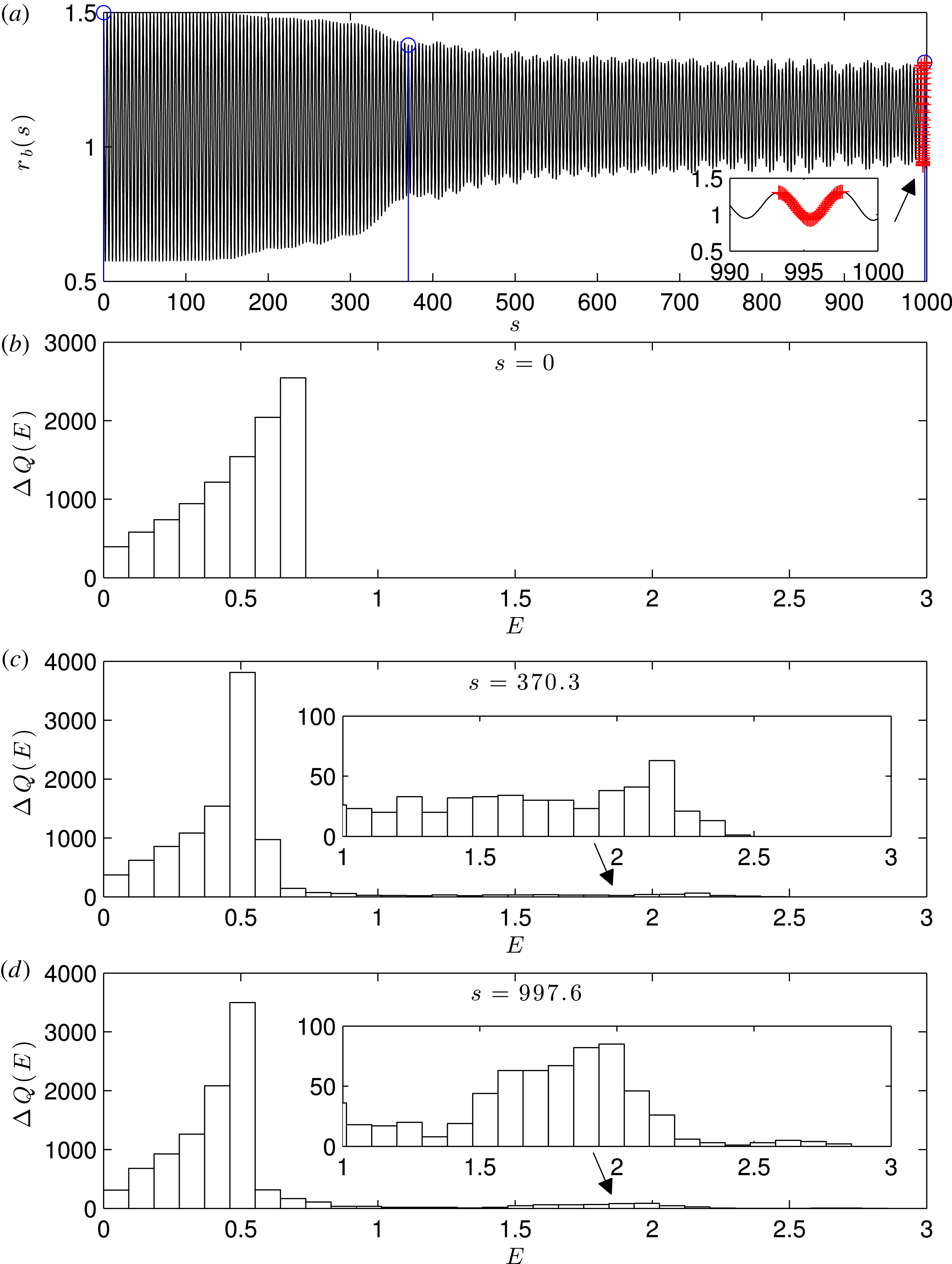
Results obtained with self-consistent numerical simulations for an initial beam mismatch of $r_{bo}=1.5$ . (a) Shows the results for the beam envelope $r_{b}(s)$ . The energy histograms $\unicode[STIX]{x0394}Q(E)$ are shown in (b) for $s=0$ , (c) for $s=370.3$ and (d) for $s=997.6$ . The width of the bins is $\unicode[STIX]{x0394}E=0.0921$ .

The figure 1 presents the dynamics of a beam with an initial mismatch of $r_{bo}=1.5$ . To macroscopically evaluate the dynamics of the beam states, figure 1(a) shows the beam envelope $r_{b}$ with time $s$ . Essentially two regimes can be observed, which are concatenated by a transition. The first regime, delimited in time by the interval $0\lessapprox s\lessapprox 180$ , is characterized by a quasi-regular oscillation of amplitude $r_{bo}\cong 0.9$ . The second regime, which starts at $s\cong 400$ , is characterized by a chaotic oscillation with amplitude $r_{beq}\cong 0.4$ which remains indefinitely. Between these regimes, there is a transition, in the time range $180\lessapprox s\lessapprox 400$ . To summarize, the beam envelope $r_{b}$ has suffered a decay during the evolution of its dynamics. The energy lost by the macroscopic envelope oscillations has been converted into microscopic energy associated with the chaotic movement of the beam particles identified as being from the halo. In figure 1(a), three specific times are highlighted in blue, one for each of the abovementioned intervals of time, which are associated with the quasi-linear regime, to the transition and on to the chaotic regime. For each one of these specific times, the histograms for the energies of the beam particles are computed. The energy of each beam particle with time is calculated using (2.5), which is a dimensionless quantity, due to the rescaling technique described above, in the first paragraph of this section. Figure 1(b–d) shows the energy histograms $\unicode[STIX]{x0394}Q(E)$ for respectively $s=0$ , $s=370.3$ and $s=997.6$ , in which $E$ is a continuous quantity associated with all the $E_{n}$ values computed through (2.5). The energy histograms $\unicode[STIX]{x0394}Q(E)$ represent the total amount of charge, with energies comprised of a bin of width $\unicode[STIX]{x0394}E$ at a given time $s$ . Mathematically, $\unicode[STIX]{x0394}Q(E)=f_{E}(E)\unicode[STIX]{x0394}E$ , in which $f_{E}(E)$ is the energy distribution of the beam particles. The width of the bins in figure 1(b,c,d) is $\unicode[STIX]{x0394}E\cong 0.0921$ . From the inspection of figure 1(a), one can observe that, initially, although homogeneous in the spatial coordinates, the beam is inhomogeneous in energy. This energy histogram profile stays almost invariant until $s\cong 180$ , when an exchanging process of beam particles between energy bins starts. The figure (1 c) shows the energy histogram $\unicode[STIX]{x0394}Q(E)$ during this exchange process. It is possible to observe that the profile of the energy histogram has significantly changed, with a change in the energy location of the maximum $\unicode[STIX]{x0394}Q(E)$ and the appearance of a tail. The tail extends until $E\cong 2.5$ , which is much higher than the maximum energy found initially in figure 1(b). The exchange process continues until the chaotic regime starts, when the energy histograms $\unicode[STIX]{x0394}Q(E)$ become almost invariant. The beam is then in its equilibrium state. In the equilibrium, from figure 1(d), it is possible to observe that in fact part of tail transforms itself into a new population in the interval $1.5\lessapprox E\lessapprox 2.25$ . The energy histogram $\unicode[STIX]{x0394}Q(E)$ of this new population is detailed in the inset in figure 1(d). This new population is composed of much more energetic particles than those that initially composed the beam.

Since the energy histogram $\unicode[STIX]{x0394}Q(E)$ is a function of the time $s$ , it is thus interesting to identify from which bins of figure 1(b) (the initial beam state) the particles of the tail and of the new highly energetic population found in figure 1(d) (the equilibrium beam state) come from. One way to evaluate this is to calculate the difference between the energy histograms $\unicode[STIX]{x0394}Q_{\text{d}}$ at the initial time $s=0$ and end time $s=997.6$ , $\unicode[STIX]{x0394}Q_{\text{d}}(E)=\unicode[STIX]{x0394}Q(E,s=0)-\unicode[STIX]{x0394}Q(E,s=997.6)$ . 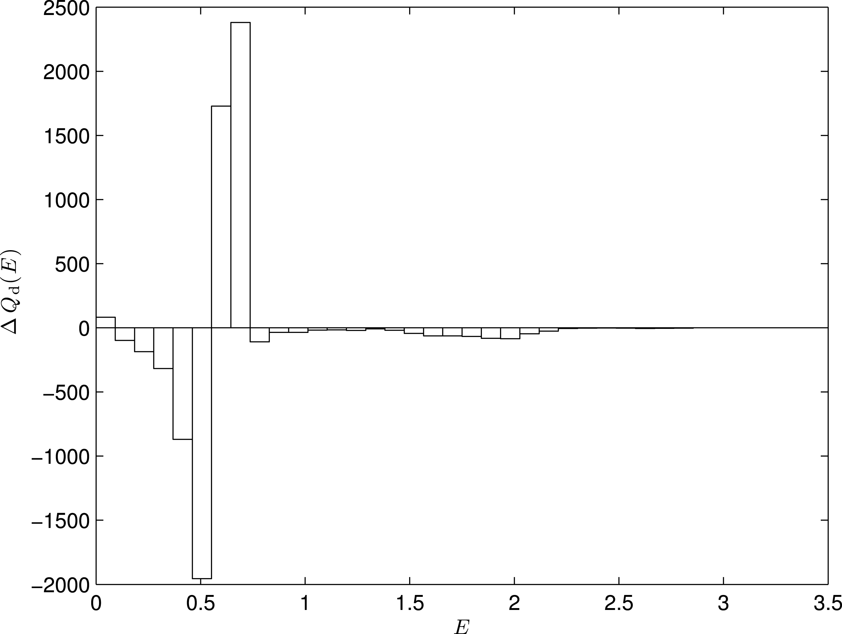Figure 2 shows the histogram for $\unicode[STIX]{x0394}Q_{\text{d}}(E)$ . Positive values of $\unicode[STIX]{x0394}Q_{\text{d}}(E)$ indicate for which energies the energy histogram of the initial state $\unicode[STIX]{x0394}Q(E,s=0)$ exceed the energy histogram of the equilibrium $\unicode[STIX]{x0394}Q(E,s=997.6)$ . It is possible to observe that, essentially, when compared with the equilibrium, the energy histogram at the initial state has a surplus of particles in two bins; $0.54605\leqslant E\leqslant 0.73025$ , and the first bin of this histogram, which has $E<0.0921$ . There is a deficit of particles in all the other values of energy. Comparing figure 1(b) with figure 2, it is possible to observe that the surplus energy values are exactly those associated with the beginning and the ending of the energy histogram at the initial beam state. These energy values are associated with the borders of the energy histogram at the initial beam state. Independently of the criteria adopted to classify particles as halo particles, since the halo is a new population of particles developed during the beam dynamics, it is possible to assert that halo particles come from the energy borders of the beam. The small amount of particles $\unicode[STIX]{x0394}Q_{\text{d}}$ with $E<0.0921$ at the initial state earns energy during the beam dynamics. Some amount of particles $\unicode[STIX]{x0394}Q_{\text{d}}$ from $0.54605\leqslant E\leqslant 0.73025$ at the initial state lose energy to populate bins with $0.0921<E<0.54605$ and some other amount of particles earns energy to populate bins with $E>0.73025$ , both at the beam equilibrium state.

Figure 2.

The difference between energy histograms at the initial state and equilibrium $\unicode[STIX]{x0394}Q_{\text{d}}(E)$ . The initial beam mismatch is $r_{bo}=1.5$ . The width of the bins is $\unicode[STIX]{x0394}E=0.0921$ .

The previous analysis accounts for the details about the dynamics of the energy histograms $\unicode[STIX]{x0394}Q(E)$ of the beam from its initial state until its equilibrium state. Notwithstanding the details discussed, the main difference between the energy histograms at the initial state and at the equilibrium state is the population of energy values higher than $E=0.73025$ . Since halo particles are highly energetic, it is possible to establish this energy value as a simple criterion to segregate halo from core particles. 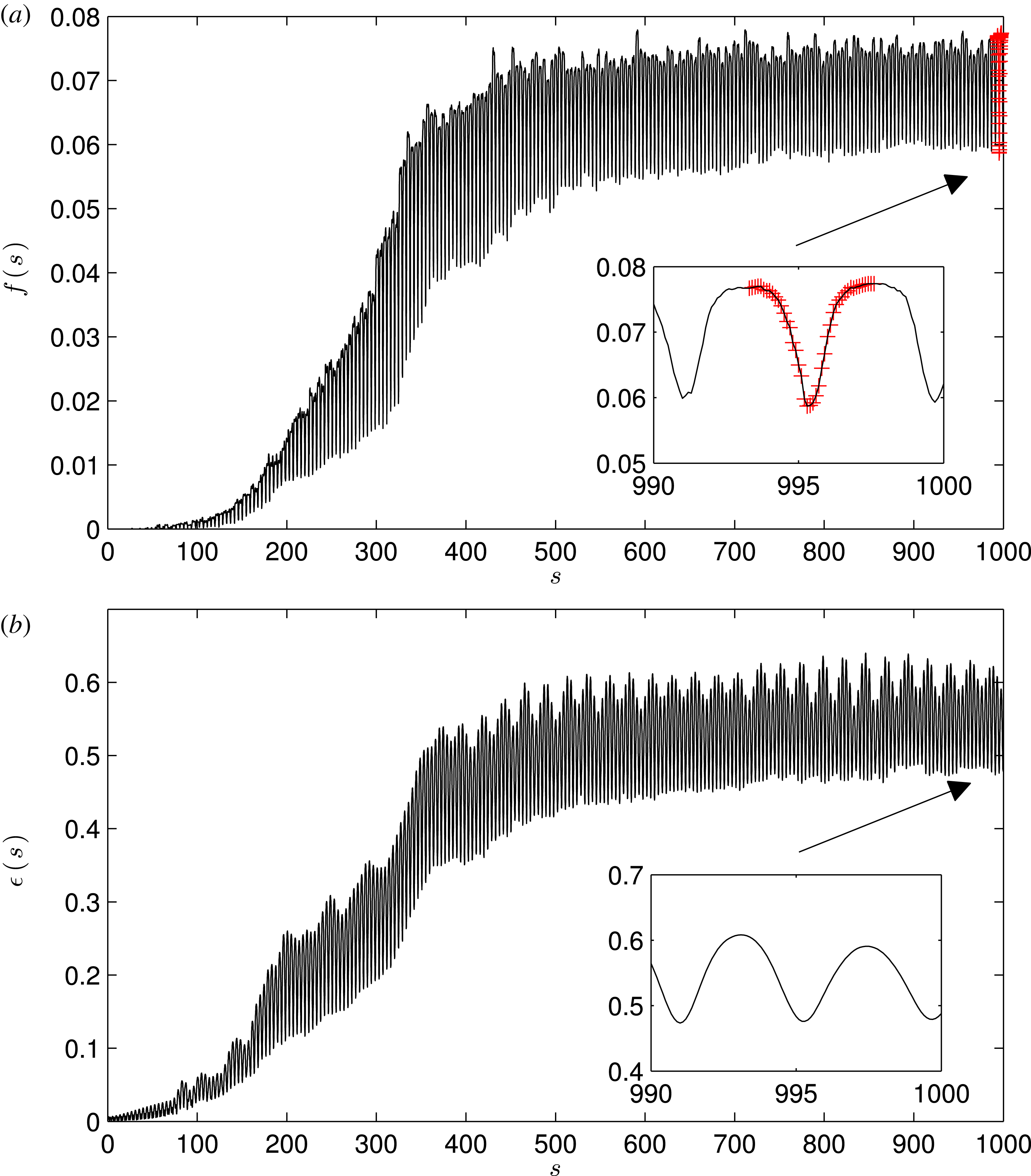Particles with energy greater than the threshold $E_{t}=0.73025$ are from the halo and those with energy smaller than the threshold $E_{t}=0.73025$ are from the core. Figure 3(a) presents the dynamics of the fraction $f$ of halo particles obtained by adopting this energy criterion. The fraction of halo particles $f$ is defined as the ratio of the total number of halo particles $N_{h}$ to the total number of beam particles $N$ , $f=N_{h}/N$ . The fraction of halo particles $f$ is almost zero until $s\cong 100$ , where an increases starts to be observed. The fraction $f$ gradually increases until $s\cong 500$ . At this time, this gradual increase ceases. This gradual increase of the fraction $f$ is consistent with the decay of the beam envelope $r_{b}(s)$ shown in figure 1(a). More, the behaviour of the fraction of halo particles $f(s)$ is very similar to the behaviour of the beam emittance $\unicode[STIX]{x1D716}(s)$ , which is plotted in figure 3(b). That is, the fraction of halo particles $f$ is strongly connected to and governs the behaviour of the beam envelope $r_{b}(s)$ and the beam emittance $\unicode[STIX]{x1D716}(s)$ .

Figure 3.

The dynamics of (a) the fraction of halo particles $f(s)$ , and (b) the beam emittance $\unicode[STIX]{x1D716}(s)$ . The initial beam mismatch is $r_{bo}=1.5$ .

During this gradual increase of the fraction $f$ shown in figure 3, in superposition an oscillatory behaviour is observed. This oscillatory behaviour means that, although in a small amount, the core exchanges particles with the halo even in equilibrium. In this way, there is an energy flux between the core and the halo at the beam equilibrium. The amplitude of this oscillation in the fraction $f$ is almost constant, implying that the resulting energy flux could be interpreted as stationary, since over a period of this oscillation the mean value of the fraction $f$ is almost constant. Due to the conservation of charge, if the halo earns particles, the core lose particles, and vice versa. This quasi-regular oscillatory behaviour of the fraction $f$ is shown in detail at the equilibrium also in figure 3, in which an inset of the interval of time $990\leqslant s\leqslant 1000$ is presented. In the inset, the values of the fraction $f$ over a period of quasi-regular oscillation is highlighted by the red ‘ $+$ ’ signs, using as the starting point the maximum local value of $f$ . The time interval associated with the highlighted values is $993.3\leqslant s\leqslant 997.6$ , being the successive maximums of the fraction $f$ at $s=993.3$ and $s=997.6$ . The dynamics of the beam envelope $r_{b}(s)$ in this interval of time is also highlighted with red ‘+’ signs in a similar inset in figure 1(a). During this time interval, the beam envelope $r_{b}(s)$ also starts and ends with consecutive local maximums. That is, a period of the beam envelope $r_{b}(s)$ is exactly the same and in phase with a period of the fraction of halo particles $f(s)$ . The oscillations in the beam envelope are controlled by the particles that compose the halo.

In fact, the energy threshold can be analytically determined for any initial beam mismatch by imposing $R_{n}=r_{bo}$ in (2.5). The total amount of charge $Q_{n}$ is calculated by inserting (2.1) into (2.4). By proceeding in this way, it is obtained that analytically

(3.1) $$\begin{eqnarray}E_{t}(r_{bo})=r_{bo}^{2}/2-\ln (r_{bo}),\end{eqnarray}$$

the energy threshold $E_{t}$ is a function of the initial beam mismatch $r_{bo}$ , which is physically reasonable.

Table 1 compares the results for the fraction of halo particles $f$ computed through the current energy criterion established by (3.1) and through the phase-space criterion adopted in past works (Nunes et al. Reference Nunes, Pakter and Rizzato2008). The comparison of the results for the fraction of halo particles $f$ occurs for the times at which the beam envelope $r_{b}(s)$ is a local maximum, since this is a restriction of the previous phase-space approach. When $r_{b}(s)$ is a local maximum, $\text{d}r_{b}(s)/\text{d}s=0$ with $\text{d}^{2}r_{b}(s)/\text{d}s^{2}<0$ , and all the core particles are over the $R$ axis of the beam phase space, it is then possible to employ the past phase-space criterion. In this way, the fraction $f$ can be only calculated when $r_{b}(s)$ is a local maximum with the phase-space criterion. This restriction does not exist in the current energy criterion, it being possible to quantify not only the gradual but also the oscillatory behaviour of the fraction $f$ . Table 1 shows that both approaches have good agreement in estimating the fraction $f$ of halo particles, for distinct values of beam initial mismatch $r_{bo}$ , except for the case of $r_{bo}=1.2$ . For $r_{bo}=1.2$ , there is a discrepancy between the approaches, which is potentially due to the width of the bin energy adopted. If a larger $N$ is used, a smaller width for the bin energy can be employed and thus it is expected that both approaches present similar values. However, this procedure is computationally costly, since for $r_{bo}=1.2$ the beam takes a long time to decay and it is then necessary to perform long-time numerical simulations. This is the reason for which results for $r_{bo}=1.1$ have not been presented. A movie with the dynamics of the energy histograms $\unicode[STIX]{x0394}Q(E,s)$ , the beam envelope $r_{b}(s)$ and the fraction of halo particles $f(s)$ from the initial beam state until the equilibrium state is included as supplementary movie for the readers available at https://doi.org/10.1017/S0022377818000284. In this movie, the initial beam mismatch is $r_{bo}=1.5$ .

Table 1.

Comparison of the results provided by the energy and the phase-space approaches for the fraction of the halo particles $f$ .

As shown, the simple energy criterion adopted has successfully segregated the halo particles from the core particles of homogeneous beams for many values of the initial envelope mismatch. The values obtained for the fraction $f$ of halo particles are in agreement with those obtained in past works in which a phase-space criterion has been adopted, except for $r_{bo}=1.2$ , as identified and discussed in the paragraph above. As a generalization, future works should take into account other beam density profiles to evaluate the extension of this simple criterion. In particular, inhomogeneous beams are of interest, since in the envelope matched situations the existence of halo particles is essentially governed by the breaking of the density waves. Further works will also consider particles evolving under periodical structures of focusing, implemented with quadrupoles and solenoids, as well as thermal aspects of the initial beam distribution, which have been neglected in the current work.