1 Background
The pulmonary epithelium is lined with a dense mat of cilia, and through coordinated beating these cilia are able to generate a steady flow in the fluid that surrounds them. Bacteria and foreign bodies which are trapped in the mucus are thus transported out of the lungs to prevent infection.
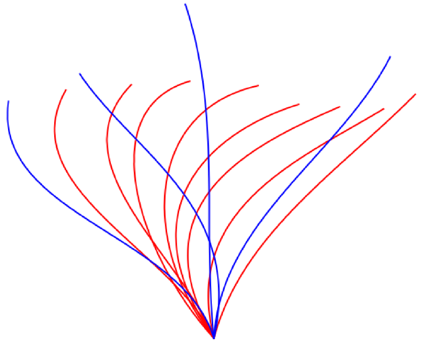
Cilia beat in an asymmetric pattern to produce a net flow in one direction. This beat pattern consists of an active stroke and a recovery stroke. During the active stroke the cilium is fully extended and rotates about its base in the direction of flow. For the recovery stroke the cilium bends and rotates more slowly in the opposite direction, returning to its starting position (Fulford & Blake Reference Fulford and Blake1986). We generate this beat profile in our model by representing each point along the length of a cilium by a truncated Fourier series with an array of coefficients defined by Fulford & Blake (Reference Fulford and Blake1986). A superposition of our cilium beat profile is shown in figure 1.
A superposition of the cilium beat pattern showing active (blue) and recovery (red) strokes. This pattern was first described mathematically by Fulford & Blake (Reference Fulford and Blake1986).

It has been observed that an array of cilia do not beat in synchrony, but there is a fixed phase step between the beat cycles of adjacent cilia (Feriani et al. Reference Feriani, Juenet, Fowler, Bruot, Chioccioli, Holland, Bryant and Cicuta2017). In large arrays of cilia this behaviour forms a metachronal wave that travels through the cilium array. In vitro the metachronal wave has been observed to be antiplectic, moving in the opposite direction to the active stroke of the cilia (Fulford & Blake Reference Fulford and Blake1986), as opposed to a symplectic wave that would move in the same direction as the active stroke. The wavelength of this metachronal wave is directly related to the size of the phase step between adjacent cilia.
Previous studies in this area have identified that a cilium array that beats with a metachronal wave can generate fluid flow much more effectively than an array that beats in synchrony, and that there is a distinctive relationship between fluid flow and metachronal wavelength (Ding et al. Reference Ding, Nawroth, McFall-Ngai and Kanso2014; Chateau et al. Reference Chateau, Favier, D’Ortona and Poncet2017). In the work of Chateau et al. (Reference Chateau, Favier, D’Ortona and Poncet2017) they postulate that the higher fluid flow generated by antiplectic cilium beating is due to the clustering of cilia during the recovery stroke, which would minimise their impact on fluid flow. The work that we present here seeks to expand on this idea by first confirming that the relationship between fluid flow and metachronal wavelength holds true for cilium spacings that are closer to values observed in pulmonary cilia (Gheber & Priel Reference Gheber and Priel1997), and then quantifying the observed behaviour with an analytical model.
2 Simulation methods
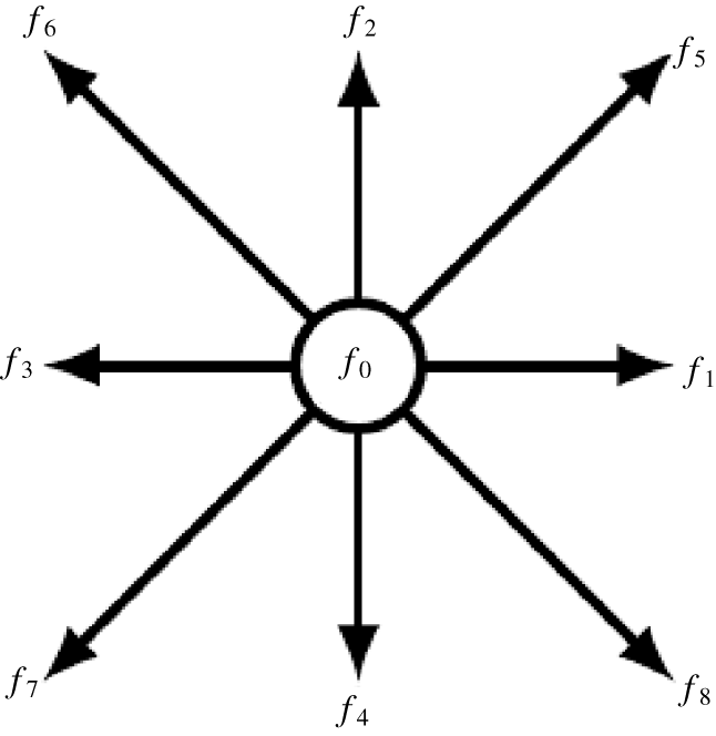
The lattice Boltzmann method is based on the idea that a fluid can be discretised as an array of static Eulerian nodes, these nodes are assigned an array of lattice vectors that point in the direction of the adjacent nodes (Kruger et al. Reference Kruger, Kusumaatmaja, Kuzmin, Shardt, Silva and Viggen2017). In two dimensions it is standard practice to assign nine vectors to each node as shown in figure 2, forming what is called a D2Q9 lattice. The magnitude of each component  $f_{i}(\boldsymbol{x},t)$ represents a certain amount of the population density of the fluid at that node. The evolution of population densities at each time step is governed by the lattice Boltzmann evolution equation
 $$\begin{eqnarray}f_{i}(\boldsymbol{x}+\boldsymbol{c}_{\boldsymbol{i}},t+1)-f_{i}(\boldsymbol{x},t)=\unicode[STIX]{x1D6FA}_{i}(\boldsymbol{x},t),\end{eqnarray}$$
where  $\boldsymbol{c}_{i}$ represents the lattice vectors assigned to each fluid node. This means that with each time step the streaming of particle density to an adjacent node in the direction of its lattice vector is modified by some collision operator
 $\unicode[STIX]{x1D6FA}_{i}(\boldsymbol{x},t)$. The simplest form of the collision operator is the Bhatnagar–Gross–Krook (BGK) collision operator (Kruger et al. Reference Kruger, Kusumaatmaja, Kuzmin, Shardt, Silva and Viggen2017) which is given by
 $$\begin{eqnarray}\unicode[STIX]{x1D6FA}_{i}^{BGK}=-\frac{1}{\unicode[STIX]{x1D70F}}[f_{i}-f_{i}^{(0)}],\end{eqnarray}$$
A representation of the population density components assigned to each fluid node in a D2Q9 lattice Boltzmann arrangement.

where  $\unicode[STIX]{x1D70F}$ is the relaxation time of the fluid and
 $f_{i}^{(0)}$ represents the equilibrium particle distribution calculated from the fluid density
 $\unicode[STIX]{x1D70C}(\boldsymbol{x},t)$ and velocity
 $\boldsymbol{u}(\boldsymbol{x},t)$ by
 $$\begin{eqnarray}f_{i}^{(0)}=\unicode[STIX]{x1D70C}\unicode[STIX]{x1D714}_{i}\left[1+\frac{\boldsymbol{c}_{\boldsymbol{i}}\boldsymbol{\cdot }\boldsymbol{u}}{c_{s}^{2}}+\frac{(\boldsymbol{c}_{\boldsymbol{i}}\boldsymbol{\cdot }\boldsymbol{u})^{2}}{2c_{s}^{4}}-\frac{\boldsymbol{u}^{2}}{2c_{s}^{2}}\right],\end{eqnarray}$$
with  $\unicode[STIX]{x1D714}_{i}$ representing weight functions that are defined as part of the dimensions of the lattice, and
 $c_{s}$ representing the speed of sound in the fluid which in this model is set as
 $c_{s}=1/\sqrt{3}$. The inclusion of immersed boundaries requires a body force term
 $F_{i}(\boldsymbol{x},t)$ to be added to (2.1), meaning that the modified evolution equation becomes
 $$\begin{eqnarray}f_{i}^{(1)}=\left(1-\frac{1}{\unicode[STIX]{x1D70F}}\right)f_{i}+\frac{1}{\unicode[STIX]{x1D70F}}f_{i}^{(0)}+F_{i},\end{eqnarray}$$
where  $f_{i}^{(1)}=f_{i}(\boldsymbol{x}+\boldsymbol{c}_{\boldsymbol{i}},t+1)$. Equation (2.4) represents the backbone of this numerical model, controlling the streaming of fluid between time steps as well as the collisions between fluid and boundaries. This is the immersed boundary lattice Boltzmann (IBLB) algorithm (Li et al. Reference Li, Favier, D’Ortona and Poncet2016). The macroscopic quantities of density and velocity can be calculated at each time step from
 $f_{i}$ by
 $$\begin{eqnarray}\displaystyle & \displaystyle \unicode[STIX]{x1D70C}(\boldsymbol{x},t)=\mathop{\sum }_{i}f_{i}(\boldsymbol{x},t), & \displaystyle\end{eqnarray}$$
 $$\begin{eqnarray}\displaystyle & \displaystyle \unicode[STIX]{x1D70C}(\boldsymbol{x},t)\boldsymbol{u}(\boldsymbol{x},t)=\mathop{\sum }_{i}\boldsymbol{c}_{\boldsymbol{i}}\,f_{i}(\boldsymbol{x},t)+{\textstyle \frac{1}{2}}\boldsymbol{F}, & \displaystyle\end{eqnarray}$$
where  $\boldsymbol{F}$ is the macroscopic value of the body force at each node. These values are used to define the equilibrium conditions for the next time step as in (2.3). In our model the relaxation time
 $\unicode[STIX]{x1D70F}$ is intrinsically linked to the Reynolds number of the system such that
 $$\begin{eqnarray}Re=\frac{UN}{c_{s}^{2}(\unicode[STIX]{x1D70F}-1/2)},\end{eqnarray}$$
where  $U$ is the characteristic speed in lattice units per time step which in this case is the average speed of a cilium tip, and
 $N$ is the characteristic length in lattice units which is the length of a cilium (Kruger et al. Reference Kruger, Kusumaatmaja, Kuzmin, Shardt, Silva and Viggen2017).
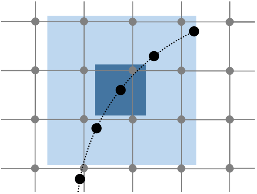
An example of a set of Lagrangian points representative of an immersed boundary (black) shown with a set of Eulerian fluid nodes (grey), including the support domain of a single boundary point.

The body force acting on the fluid can be determined by first defining a series of Lagrangian points which are representative of the surface geometry, as demonstrated in figure 3 (Li et al. Reference Li, Favier, D’Ortona and Poncet2016).
The interaction between the fluid nodes and surface points is calculated by interpolating equation (2.6), resulting in the equation
 $$\begin{eqnarray}\boldsymbol{F}_{\boldsymbol{s}}=\mathop{\sum }_{j\in D_{s}}2\unicode[STIX]{x1D70C}_{j}\tilde{\unicode[STIX]{x1D6FF}}(\boldsymbol{x}_{\boldsymbol{j}}-\boldsymbol{x}_{\boldsymbol{s}})(\boldsymbol{u}_{\boldsymbol{s}}-\boldsymbol{u}_{\boldsymbol{j}}),\end{eqnarray}$$
which determines the force of the fluid acting on a single surface point  $F_{s}$ based on the difference between the surface velocity
 $u_{s}$ and the fluid velocity
 $u_{j}$ at nodes within the support domain of the surface point
 $D_{s}$ (Pinelli et al. Reference Pinelli, Naqavi, Piomelli and Favier2010). The contribution from each node is scaled by a smoothed delta function
 $\tilde{\unicode[STIX]{x1D6FF}}(\boldsymbol{x}_{\boldsymbol{j}}-\boldsymbol{x}_{\boldsymbol{s}})$ which takes the form
 $$\begin{eqnarray}\tilde{\unicode[STIX]{x1D6FF}}(\boldsymbol{x}_{\boldsymbol{j}}-\boldsymbol{x}_{\boldsymbol{s}})=\tilde{\unicode[STIX]{x1D6FF}_{x}}(|x_{j}-x_{s}|)\tilde{\unicode[STIX]{x1D6FF}_{y}}(|y_{j}-y_{s}|),\end{eqnarray}$$
with
 $$\begin{eqnarray}\tilde{\unicode[STIX]{x1D6FF}}_{x,y}(r)=\left\{\begin{array}{@{}ll@{}}\frac{1}{3}\left(1+\sqrt{-3r^{2}+1}\right),\quad & 0\leqslant r\leqslant 0.5,\\ \frac{1}{6}\left[5-3r-\sqrt{-3(1-r)^{2}+1}\right],\quad & 0.5\leqslant r\leqslant 1.5,\\ 0\quad & \text{otherwise}.\end{array}\right.\end{eqnarray}$$
The delta function also serves to define the support domain of each surface point as a square of side 3 lattice units centred at that point, as shown in figure 3 (Li et al. Reference Li, Favier, D’Ortona and Poncet2016). The force at the surface points is then spread to the surrounding fluid nodes by way of the relation
 $$\begin{eqnarray}\boldsymbol{F}(\boldsymbol{x}_{\boldsymbol{j}},t)=\mathop{\sum }_{s\in D_{j}}\boldsymbol{F}_{\boldsymbol{s}}\tilde{\unicode[STIX]{x1D6FF}}(\boldsymbol{x}_{\boldsymbol{j}}-\boldsymbol{x}_{\boldsymbol{s}})\unicode[STIX]{x0394}s,\end{eqnarray}$$
which calculates the body force at point  $j$ as the sum of the surface forces from all surface points within the support domain
 $D_{j}$ (Pinelli et al. Reference Pinelli, Naqavi, Piomelli and Favier2010), scaled by the same delta function as described in (2.9), and the surface point separation
 $\unicode[STIX]{x0394}s$. The macroscopic body force
 $\boldsymbol{F}$ is used to modify the velocity of the affected fluid nodes through (2.6). It can also be broken down into lattice vector components for each node using
 $$\begin{eqnarray}F_{i}=\left(1-\frac{1}{2\unicode[STIX]{x1D70F}}\right)\unicode[STIX]{x1D714}_{i}\left[\frac{\boldsymbol{c}_{\boldsymbol{i}}-\boldsymbol{u}}{{c_{s}}^{2}}+\frac{\boldsymbol{c}_{\boldsymbol{i}}\boldsymbol{\cdot }\boldsymbol{u}}{{c_{s}}^{4}}\boldsymbol{c}_{\boldsymbol{i}}\right]\boldsymbol{\cdot }\boldsymbol{F}.\end{eqnarray}$$
This discrete force is used in (2.1) to modify the collision operator to include the body force associated with the immersed boundary. It should be noted that all of the above equations are written in lattice units so that the lattice spacing ( $\unicode[STIX]{x0394}x$) and the time step size (
 $\unicode[STIX]{x0394}t$) are equal to unity. The scaled value of
 $\unicode[STIX]{x0394}x$ is fixed throughout the work reported here such that
 $\unicode[STIX]{x0394}x=62.5~\text{nm}$ to ensure that the characteristic length is approximately 100 lattice units. The time step size is varied depending on the Reynolds number to maintain an optimal relaxation time and to keep the fluid velocity significantly lower than the speed of sound on the lattice (Kruger et al. Reference Kruger, Kusumaatmaja, Kuzmin, Shardt, Silva and Viggen2017). Unless otherwise stated we set the Reynolds number to be equal to unity, meaning that the scaled time step size is also fixed such that
 $\unicode[STIX]{x0394}t=66.7~\text{ns}$. We note that using this time step size means that simulating a full cilium beat cycle (
 $T=66.7~\text{ms}$) requires
 $10^{6}$ time steps. This is necessary to maintain the accuracy of our simulations.
Due to the low Reynolds number of the system that we are modelling ( $Re\leqslant 1$), we have used the two relaxation time (TRT) method to avoid significant inaccuracies in our simulations (Kruger et al. Reference Kruger, Kusumaatmaja, Kuzmin, Shardt, Silva and Viggen2017). In the case of the BGK collision operator the accuracy of a simulation increases proportionally with
 $\unicode[STIX]{x1D70F}$, and to increase the viscosity of our fluid we must increase
 $\unicode[STIX]{x1D70F}$. The TRT method allows us to alter the viscosity of our fluid without directly affecting the accuracy of our simulations through the use of a second relaxation time. In this case the accuracy of a simulation is tied to a so called magic parameter
 $\unicode[STIX]{x1D6EC}$ which is defined by
 $$\begin{eqnarray}\unicode[STIX]{x1D6EC}=\left(\unicode[STIX]{x1D70F}^{+}-{\textstyle \frac{1}{2}}\right)\left(\unicode[STIX]{x1D70F}^{-}-{\textstyle \frac{1}{2}}\right),\end{eqnarray}$$
where  $\unicode[STIX]{x1D70F}^{+}$ dictates the viscosity of our fluid in the same way as
 $\unicode[STIX]{x1D70F}$ for the BGK collision operator, and
 $\unicode[STIX]{x1D70F}^{-}$ is a free parameter. By fixing
 $\unicode[STIX]{x1D6EC}$ we ensure that the accuracy of our simulations does not increase due to instability or truncation errors when we increase viscosity. We use a value of
 $\unicode[STIX]{x1D6EC}=1/12$ to optimise our simulations for pure advection problems (Kruger et al. Reference Kruger, Kusumaatmaja, Kuzmin, Shardt, Silva and Viggen2017). The standard implementation of the TRT method is based on the fact that for each velocity component
 $\boldsymbol{c}_{i}$ there is an opposing component where
 $\boldsymbol{c}_{\overline{i}}=-\boldsymbol{c}_{i}$ (Kruger et al. Reference Kruger, Kusumaatmaja, Kuzmin, Shardt, Silva and Viggen2017). This is used to generate symmetric and antisymmetric parts of the population by
 $$\begin{eqnarray}f_{i}^{+}=\frac{f_{i}+f_{\overline{i}}}{2},\quad f_{i}^{-}=\frac{f_{i}-f_{\overline{i}}}{2}.\end{eqnarray}$$
Similarly for the equilibrium population
 $$\begin{eqnarray}f_{i}^{(0)+}=\frac{f_{i}^{(0)}+f_{\overline{i}}^{(0)}}{2},\quad f_{i}^{(0)-}=\frac{f_{i}^{(0)}-f_{\overline{i}}^{(0)}}{2}.\end{eqnarray}$$
The symmetric and antisymmetric populations are used in an alternative collision operator to the BGK method shown in (2.2) where
 $$\begin{eqnarray}\unicode[STIX]{x1D6FA}_{i}^{TRT}=-\frac{1}{\unicode[STIX]{x1D70F}^{+}}(f_{i}^{+}-f_{i}^{(0)+})-\frac{1}{\unicode[STIX]{x1D70F}^{-}}(f_{i}^{-}-f_{i}^{(0)-}).\end{eqnarray}$$
We use the TRT method to ensure that when we simulate fluid at low Reynolds numbers ( $Re<1$) the increase in viscosity does not alter the accuracy of our results.
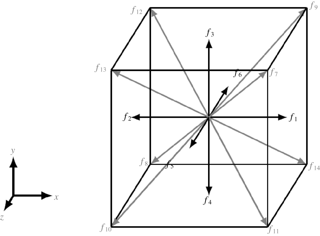
In our three-dimensional (3-D) model we use the same lattice Boltzmann algorithm as described above, only with a 3-D arrangement of fluid nodes that each have 15 components (D3Q15) as shown in figure 4.
A representation of the population densities assigned to each node in a D3Q15 lattice Boltzmann model.

We use the immersed boundary method in our model to represent each cilium as a distribution of point forces along its length. Each cilium is made up of 96 boundary points that are separated by a single lattice unit making the thickness of each cilium less than one lattice unit. The dimensions of a simulation are always defined relative to the cilium length and the cilium spacing such that the  $x$ dimension is given by the cilium spacing multiplied by the number of cilia and the y dimension is double the cilium length.
In our simulations cilia are free to move past one another, but this means that boundary points can come into very close proximity. To avoid problems caused by this, our model checks for boundary points that are too close together and deactivates one of the points. Cilia moving past one another also generates closed fluid regions in 2-D simulations, but we avoid changes in the fluid density in these regions by allowing fluid to flow in or out of these regions at the base of the cilia. Introducing this into the model has minimal effect on the results of our simulations, and allows us to explore a wider range of parameters.
Our model is written in CUDA so that we can perform simulations in parallel on a GPU, specifically we have been running simulations on an Nvidia TESLA K80 graphics card. The IBLB algorithm is well suited to parallel programming due to the calculations for each time step being completely localised (Kruger et al. Reference Kruger, Kusumaatmaja, Kuzmin, Shardt, Silva and Viggen2017).
Cilium simulation parameters.

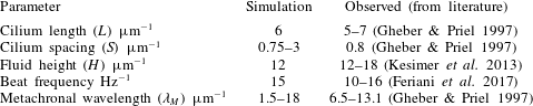
We have selected specific parameters for our simulations to ensure that our model is representative of the in vivo system. Parameters such as the cilium length, cilium spacing and fluid height have been well documented through electron microscopy in the literature (Gheber & Priel Reference Gheber and Priel1997; Kesimer et al. Reference Kesimer, Ehre, Burns, Davis, Sheehan and Pickles2013). Some of the mechanical parameters such as the cilium beat frequency and metachronal wavelength are less well defined in the biological system (Gheber & Priel Reference Gheber and Priel1997; Feriani et al. Reference Feriani, Juenet, Fowler, Bruot, Chioccioli, Holland, Bryant and Cicuta2017). We have selected a beat frequency to optimise cilium driven fluid flow, and a range of metachronal wavelengths that allow us to investigate how this parameter affects fluid flow. The major physical parameters are summarised in table 1.
The boundary conditions of our model consist of a no-slip boundary at the bottom (epithelium), a free-slip boundary at the top (air interface) and periodic boundaries at the left and right edges of the fluid region so that we can generate a continuous flow of fluid. The boundary points of the cilia also obey the periodic boundary condition so that we can represent a large and continuous array of cilia with relatively few discretely modelled cilia.
The scale of the system relative to the viscosity of water  $(\unicode[STIX]{x1D708}\approx 8\times 10^{-7}~\text{m}^{2}~\text{s}^{-1})$ means that the Reynolds number is very small
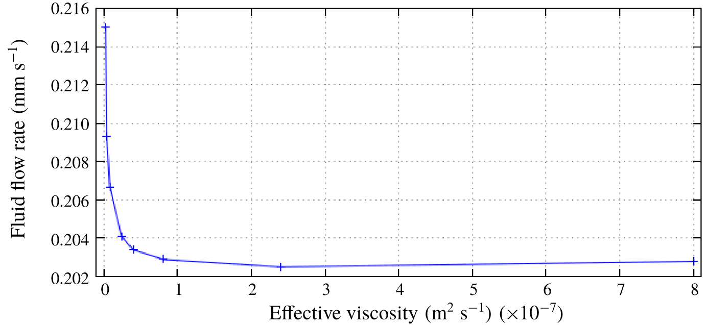
 $(Re\approx 0.003)$, but achieving significant and accurate results from our model with this Reynolds number would be infeasible because the time step must be decreased in proportion with the Reynolds number. We have conducted a series of convergence tests to determine a suitable Reynolds number that would allow us to run simulations quickly without sacrificing the accuracy of the model. We found that simulations using
 $Re=1\;(\unicode[STIX]{x1D708}\approx 2.4\times 10^{-9}~\text{m}^{2}~\text{s}^{-1})$ display identical behaviour with comparable flow rates to those given by simulations using
 $Re=0.003\;(\unicode[STIX]{x1D708}\approx 8\times 10^{-7}~\text{m}^{2}~\text{s}^{-1})$, with a significant reduction in run time. Results from these convergence tests are shown in figure 5. Based on the results of these convergence tests, we use a value of
 $Re=1$ in all of our simulations.
Results from convergence tests to justify using a numerical Reynolds number  $Re=1\;(\unicode[STIX]{x1D708}\approx 2.4\times 10^{-9}~\text{m}^{2}~\text{s}^{-1})$ to represent the biological system where
 $Re\approx 0.003\;(\unicode[STIX]{x1D708}\approx 8\times 10^{-7}~\text{m}^{2}~\text{s}^{-1})$.

In our simulations the cilium beat pattern is completely prescribed, which means that the motion of the fluid has no effect on the cilium motion. This allows us to control the metachronal wavelength ( $\unicode[STIX]{x1D706}_{M}$) in the cilium array by varying the phase step (
 $\unicode[STIX]{x0394}\unicode[STIX]{x1D719}=2\unicode[STIX]{x03C0}S/\unicode[STIX]{x1D706}_{M}$) which corresponds to a time delay between the beat cycles of adjacent cilia. We have been able to confirm that due to the periodic boundary conditions the fluid flow rate is independent of the extent of the modelled fluid region, i.e. the
 $x$ dimension of the fluid region and the number of cilia that are included, so long as the cilium spacing and phase step are kept constant. These results are included in appendix A.
The 3-D version of the model eliminates any abnormalities present in a 2-D fluid, and gives us results that more closely represent the biological system that we are modelling. Our 3-D model uses the same periodic boundary conditions in the third dimension to represent multiple rows of cilia beating parallel to one another. Run times for our 3-D simulations are significantly longer which limits the range of parameters that we can investigate, so for the purposes of this study we have used a smaller number of 3-D simulations to verify that the results of our 2-D simulations are representative of the 3-D system.
3 Observations
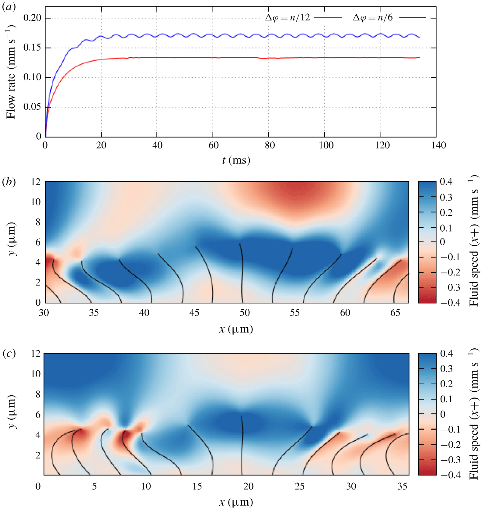
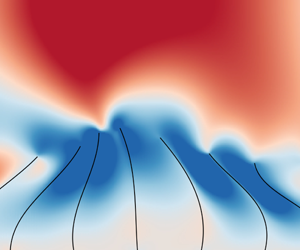
(a) A comparison of flow rates resulting from cilium beats with different phase step values:  $\unicode[STIX]{x0394}\unicode[STIX]{x1D719}=\unicode[STIX]{x03C0}/12$ (red),
 $\unicode[STIX]{x0394}\unicode[STIX]{x1D719}=\unicode[STIX]{x03C0}/6$ (blue). Cilium spacing is
 $3~\unicode[STIX]{x03BC}\text{m}$ in both cases. (b) An example of the cilium profiles and fluid flow for
 $\unicode[STIX]{x0394}\unicode[STIX]{x1D719}=\unicode[STIX]{x03C0}/12$. Colour box represents fluid speed in the
 $x+$ direction. Figure shows a trimmed section of a larger fluid region. (c) An example of the cilium profiles and fluid flow for
 $\unicode[STIX]{x0394}\unicode[STIX]{x1D719}=\unicode[STIX]{x03C0}/6$. Colour box represents fluid speed in the
 $x+$ direction.

During some initial simulations using our IBLB model, we observed that the fluid flow rate was dependent on the phase step and by varying the value of  $\unicode[STIX]{x0394}\unicode[STIX]{x1D719}$ we could control the rate of fluid flow as shown in figure 6(a). We note that increasing the value of
 $\unicode[STIX]{x0394}\unicode[STIX]{x1D719}$ also causes an oscillation in the flow rate, due to the time delay between the active strokes of each cilium. Our results also indicated that the cilium array was most effective at driving fluid flow when the tips of the cilia were more widely spaced during their active stroke. As an example the flow rate recorded for
 $\unicode[STIX]{x0394}\unicode[STIX]{x1D719}=\unicode[STIX]{x03C0}/6$ was significantly faster than for
 $\unicode[STIX]{x0394}\unicode[STIX]{x1D719}=\unicode[STIX]{x03C0}/12$, and there is a visible difference between the cilium spread in these two cases as shown in figures 6(b) and 6(c).
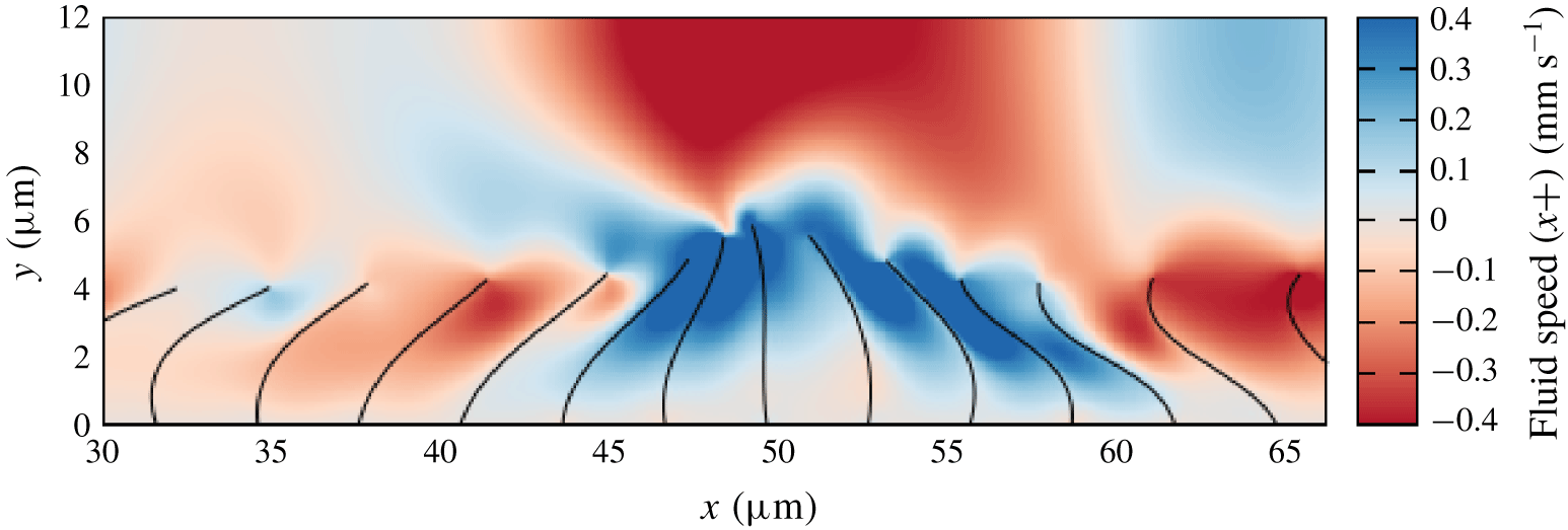
An extreme case of this behaviour occurs when  $\unicode[STIX]{x0394}\unicode[STIX]{x1D719}=23\unicode[STIX]{x03C0}/12$. Figure 7 shows that in this case the cilia are very closely clustered together during the active stroke and spread out during the recovery stroke. This means that the recovery stroke drives the fluid more effectively than the active stroke, and the resulting fluid flow is in the opposite direction to what we expect. This behaviour has also been observed in recent simulations (Khaderi, den Toonder & Onck Reference Khaderi, den Toonder and Onck2011; Chateau et al. Reference Chateau, Favier, D’Ortona and Poncet2017), with the reasoning that when the cilia are spread out each cilium is able to transfer more energy to the fluid (Chateau et al. Reference Chateau, Favier, D’Ortona and Poncet2017). By running simulations with a cilium spacing that is representative of pulmonary cilia we can obtain a more detailed understanding of this behaviour and how it relates to cilia in vivo. We can also quantify the behaviour using a simple analytical model of the cilium system.
An example of the cilium clustering during their active stroke when $\unicode[STIX]{x0394}\unicode[STIX]{x1D719}=23\unicode[STIX]{x03C0}/12$. Figure shows a trimmed section of a larger fluid region. Colour bar represents fluid speed in the
 $x+$ direction.

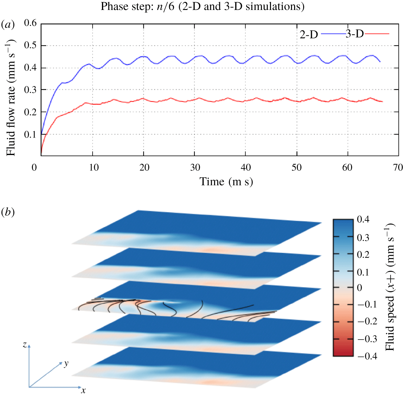
We can also compare the fluid flow rate from 2-D and 3-D simulations for the same phase step to show that both models represent the same behaviour, as we can see in figure 8(a). The only major difference between the two results is that the flow rate in the 3-D case is slower than in the 2-D case. This is as expected since the 2-D model represents infinite rows of cilia with no space between them, where as the 3-D model includes space between the rows of cilia which reduces the effectiveness of each cilium stroke. Figure 8(b) shows similar fluid behaviour exhibited in our 3-D simulations.
(a) A comparison of flow rates resulting from cilium beats in both a 2-D (blue) and a 3-D (red) fluid region. (b) An example of fluid flow in three dimensions showing similar behaviour to 2-D model.

4 Analytical model
To determine the physical principles of how the grouping of cilia can affect fluid flow rate, we have formulated a simple analytical model of the cilium array. We assume that each cilium remains straight throughout its beat cycle and moves through an active stroke where the cilium is fully extended moving through a  $90^{\circ }$ arc, and a recovery stroke where the cilium moves at half-speed with a reduced length back to its initial position.
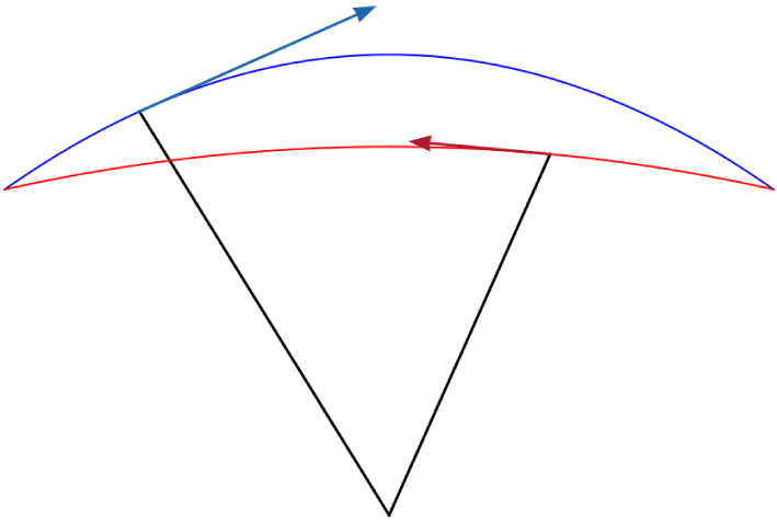
This type of analytical model was first proposed by Barton & Raynor (Reference Barton and Raynor1967), although the cilium beat profile in our model is different in a few key ways. The cilia in our model rotate about the base such that the cilium tip sweeps an arc through the active stroke rather than moving parallel to the epithelial plane. Rather than shortening instantaneously our cilia retract and extend during the recovery stroke so that the beat profile is continuous at the transition between the two strokes as shown in figure 9.
A graphical representation of the beat cycle of a single cilium in our analytical model. We have plotted a trace of the active stroke (blue) and the recovery stroke (red) for a full period of the phase angle ( $0\leqslant \unicode[STIX]{x1D719}\leqslant 2\unicode[STIX]{x03C0}$).

The position of each cilium tip relative to its base is calculated as a function of the beat phase  $(0\leqslant \unicode[STIX]{x1D719}\leqslant 2\unicode[STIX]{x03C0})$. For the active stroke
 $(0\leqslant \unicode[STIX]{x1D719}<2\unicode[STIX]{x03C0}/3)$ the position of the cilium tip is given by
 $$\begin{eqnarray}x(\unicode[STIX]{x1D719})=\frac{-\sqrt{2}L}{2}\cos \left(\frac{3}{2}\unicode[STIX]{x1D719}\right)\end{eqnarray}$$
for the  $x$ coordinate, and
 $$\begin{eqnarray}y(\unicode[STIX]{x1D719})=\frac{L}{2}\left[1+\frac{\sqrt{2}}{2}+\left(\frac{\sqrt{2}}{2}-1\right)\cos \left(3\unicode[STIX]{x1D719}\right)\right]\end{eqnarray}$$
for the  $y$ coordinate. Similarly for the recovery stroke
 $(2\unicode[STIX]{x03C0}/3\leqslant \unicode[STIX]{x1D719}<2\unicode[STIX]{x03C0})$ the position is given by
 $$\begin{eqnarray}x(\unicode[STIX]{x1D719})=\frac{2\sqrt{2}L}{5}\sin \left(\frac{3}{4}\unicode[STIX]{x1D719}\right)\end{eqnarray}$$
and
 $$\begin{eqnarray}y(\unicode[STIX]{x1D719})={\textstyle \frac{8+5\sqrt{2}}{20}}L+{\textstyle \frac{8-5\sqrt{2}}{20}}L\cos \left({\textstyle \frac{3}{2}}\unicode[STIX]{x1D719}\right).\end{eqnarray}$$
This generates a continuous beat profile that is geometrically symmetrical but has a recovery stroke that is half the speed of the active stroke, which is a key factor in the cilium beat cycle. A graphical representation of this beat cycle is shown in figure 9. We can calculate the position of each cilium tip relative to a specific cilium (cilium 0) by taking the phase of each cilium to be
 $$\begin{eqnarray}\unicode[STIX]{x1D719}_{n}=\unicode[STIX]{x1D719}_{0}+n\unicode[STIX]{x0394}\unicode[STIX]{x1D719},\end{eqnarray}$$
where  $\unicode[STIX]{x1D719}_{0}$ is the phase of cilium 0. By substituting this relationship into (4.1)–(4.4) and accounting for the cilium spacing
 $S$, for the active stroke
 $\left(0\leqslant (\unicode[STIX]{x1D719}_{0}+n\unicode[STIX]{x0394}\unicode[STIX]{x1D719})<2\unicode[STIX]{x03C0}/3\right)$ the position of each cilium tip relative to cilium 0 is given by
 $$\begin{eqnarray}x_{n}(\unicode[STIX]{x1D719}_{0},\unicode[STIX]{x0394}\unicode[STIX]{x1D719})=nS+\frac{-\sqrt{2}L}{2}\cos \left[\frac{3}{2}(\unicode[STIX]{x1D719}_{0}+n\unicode[STIX]{x0394}\unicode[STIX]{x1D719})\right]\end{eqnarray}$$
for the  $x$ coordinate, and
 $$\begin{eqnarray}y_{n}(\unicode[STIX]{x1D719}_{0},\unicode[STIX]{x0394}\unicode[STIX]{x1D719})=\frac{L}{2}\left[1+\frac{\sqrt{2}}{2}+\left(\frac{\sqrt{2}}{2}-1\right)\cos [3(\unicode[STIX]{x1D719}_{0}+n\unicode[STIX]{x0394}\unicode[STIX]{x1D719})]\right]\end{eqnarray}$$
for the  $y$ coordinate. Similarly, for the recovery stroke
 $(2\unicode[STIX]{x03C0}/3\leqslant (\unicode[STIX]{x1D719}_{0}+n\unicode[STIX]{x0394}\unicode[STIX]{x1D719})<2\unicode[STIX]{x03C0})$ the position is given by
 $$\begin{eqnarray}x_{n}(\unicode[STIX]{x1D719}_{0},\unicode[STIX]{x0394}\unicode[STIX]{x1D719})=nS+\frac{2\sqrt{2}L}{5}\sin \left[\frac{3}{4}(\unicode[STIX]{x1D719}_{0}+n\unicode[STIX]{x0394}\unicode[STIX]{x1D719})\right],\end{eqnarray}$$
and
 $$\begin{eqnarray}y_{n}(\unicode[STIX]{x1D719}_{0},\unicode[STIX]{x0394}\unicode[STIX]{x1D719})={\textstyle \frac{8+5\sqrt{2}}{20}}L+{\textstyle \frac{8-5\sqrt{2}}{20}}L\cos \left[{\textstyle \frac{3}{2}}(\unicode[STIX]{x1D719}_{0}+n\unicode[STIX]{x0394}\unicode[STIX]{x1D719})\right].\end{eqnarray}$$
We can reason that the most important case for our investigation is when cilium 0 is half-way through its active stroke ( $\unicode[STIX]{x1D719}_{0}=\unicode[STIX]{x03C0}/3$), because this is when a cilium would be moving fastest and driving fluid flow most effectively. By focusing on this static case and by modifying (4.6)–(4.9) we can deduce that for the active stroke (
 $5\unicode[STIX]{x03C0}/3\leqslant \unicode[STIX]{x0394}\unicode[STIX]{x1D719}<2\unicode[STIX]{x03C0}$ and
 $0\leqslant \unicode[STIX]{x0394}\unicode[STIX]{x1D719}<\unicode[STIX]{x03C0}/3$) the relative position of the tip of cilium
 $n$ is given by
 $$\begin{eqnarray}x_{n}(\unicode[STIX]{x0394}\unicode[STIX]{x1D719})=nS+\frac{\sqrt{2}L}{2}\sin \left(\frac{3}{2}n\unicode[STIX]{x0394}\unicode[STIX]{x1D719}\right),\end{eqnarray}$$
for the  $x$ coordinate, and
 $$\begin{eqnarray}y_{n}(\unicode[STIX]{x0394}\unicode[STIX]{x1D719})=\frac{L}{2}\left[1+\frac{\sqrt{2}}{2}-\left(\frac{\sqrt{2}}{2}-1\right)\cos (3n\unicode[STIX]{x0394}\unicode[STIX]{x1D719})\right],\end{eqnarray}$$
for the  $y$ coordinate. Similarly for the recovery stroke
 $(\unicode[STIX]{x03C0}/3\leqslant \unicode[STIX]{x0394}\unicode[STIX]{x1D719}<5\unicode[STIX]{x03C0}/3)$ the position is given by
 $$\begin{eqnarray}x_{n}(\unicode[STIX]{x0394}\unicode[STIX]{x1D719})=nS+\frac{2\sqrt{2}L}{5}\sin \left(\frac{\unicode[STIX]{x03C0}}{4}+\frac{3}{4}n\unicode[STIX]{x0394}\unicode[STIX]{x1D719}\right),\end{eqnarray}$$
and
 $$\begin{eqnarray}y_{n}(\unicode[STIX]{x0394}\unicode[STIX]{x1D719})={\textstyle \frac{8+5\sqrt{2}}{20}}L-{\textstyle \frac{8-5\sqrt{2}}{20}}L\sin \left({\textstyle \frac{3}{2}}n\unicode[STIX]{x0394}\unicode[STIX]{x1D719}\right).\end{eqnarray}$$
Using these equations we can calculate the distances and height differences between cilium 0 which is driving fluid flow and the other cilia which would impede that flow.
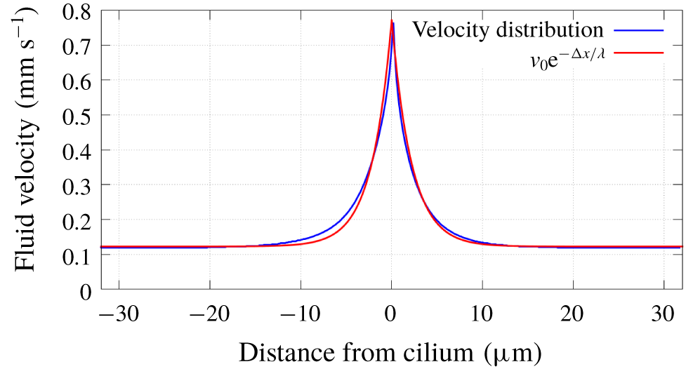
Fluid properties are represented in our analytical model by the dissipation of fluid velocity over long distances. We have characterised this by simulating a large fluid region driven by a single cilium. By measuring the fluid velocity in the horizontal plane level with the cilium tip we observed that the dissipation of fluid velocity is well explained by an exponential function of the distance from the cilium as shown in figure 10. We interpret this as the effectiveness of the cilium at a distance  $(\unicode[STIX]{x0394}x)$, and by fitting an exponential function to the velocity distribution we can find the characteristic length
 $(\unicode[STIX]{x1D706})$ of the effectiveness. Here
 $\unicode[STIX]{x1D706}$ is inversely proportional to the Reynolds number of the system for low Reynolds numbers, which represents how the force dissipation depends on viscosity. We note that this relationship breaks down for higher Reynolds numbers (
 $Re\geqslant 10$) due to the presence of vortices, meaning that the fluid velocity can no longer be described by an exponential function of distance.
Observed fluid velocity as a function of distance from the cilium. With fitted exponential function for  $\unicode[STIX]{x1D706}=2.19~\unicode[STIX]{x03BC}\text{m}$.


We calculate the effective area  $(E)$ of the active cilium by integrating the effectiveness over the full range of
 $x$
 $$\begin{eqnarray}E=2H\int _{0}^{\infty }\text{e}^{-x/\unicode[STIX]{x1D706}}\,\text{d}x,\end{eqnarray}$$
where  $H$ is the height of the fluid region. The resistance caused by the
 $n$th cilium in the array
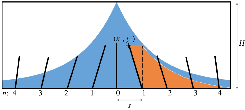
 $(R_{n})$ is calculated as the area that is blocked by that cilium using the position of the cilium base and the cilium tip
 $$\begin{eqnarray}R_{n}=y_{n}\left(\frac{nS-x_{n}}{2}+\int _{0}^{\infty }\text{e}^{-x/\unicode[STIX]{x1D706}}\,\text{d}x\right).\end{eqnarray}$$
Here, we use the same definition for the effective range of a cilium as described in figure 10. The area calculated in (4.15) is represented graphically in figure 11. We can calculate the free area  $(F)$ available to the active cilium by
 $$\begin{eqnarray}F=E-2\mathop{\sum }_{n=1}^{\infty }R_{n}\text{e}^{-nS/\unicode[STIX]{x1D706}},\end{eqnarray}$$
where we scale the resistance of each cilium exponentially with its distance from the active cilium using the same characteristic length  $(\unicode[STIX]{x1D706})$ as we determined in figure 10. This gives us an equation for free area that depends on the phase step and the cilium spacing.
 $$\begin{eqnarray}F=2H\unicode[STIX]{x1D706}-\mathop{\sum }_{n=1}^{\infty }y_{n}(nS-x_{n}+2\unicode[STIX]{x1D706})\text{e}^{-nS/\unicode[STIX]{x1D706}},\end{eqnarray}$$
where  $x_{n}=x_{n}(\unicode[STIX]{x0394}\unicode[STIX]{x1D719})$, and
 $y_{n}=y_{n}(\unicode[STIX]{x0394}\unicode[STIX]{x1D719})$ as defined in (4.10)–(4.13).
5 Results and analysis
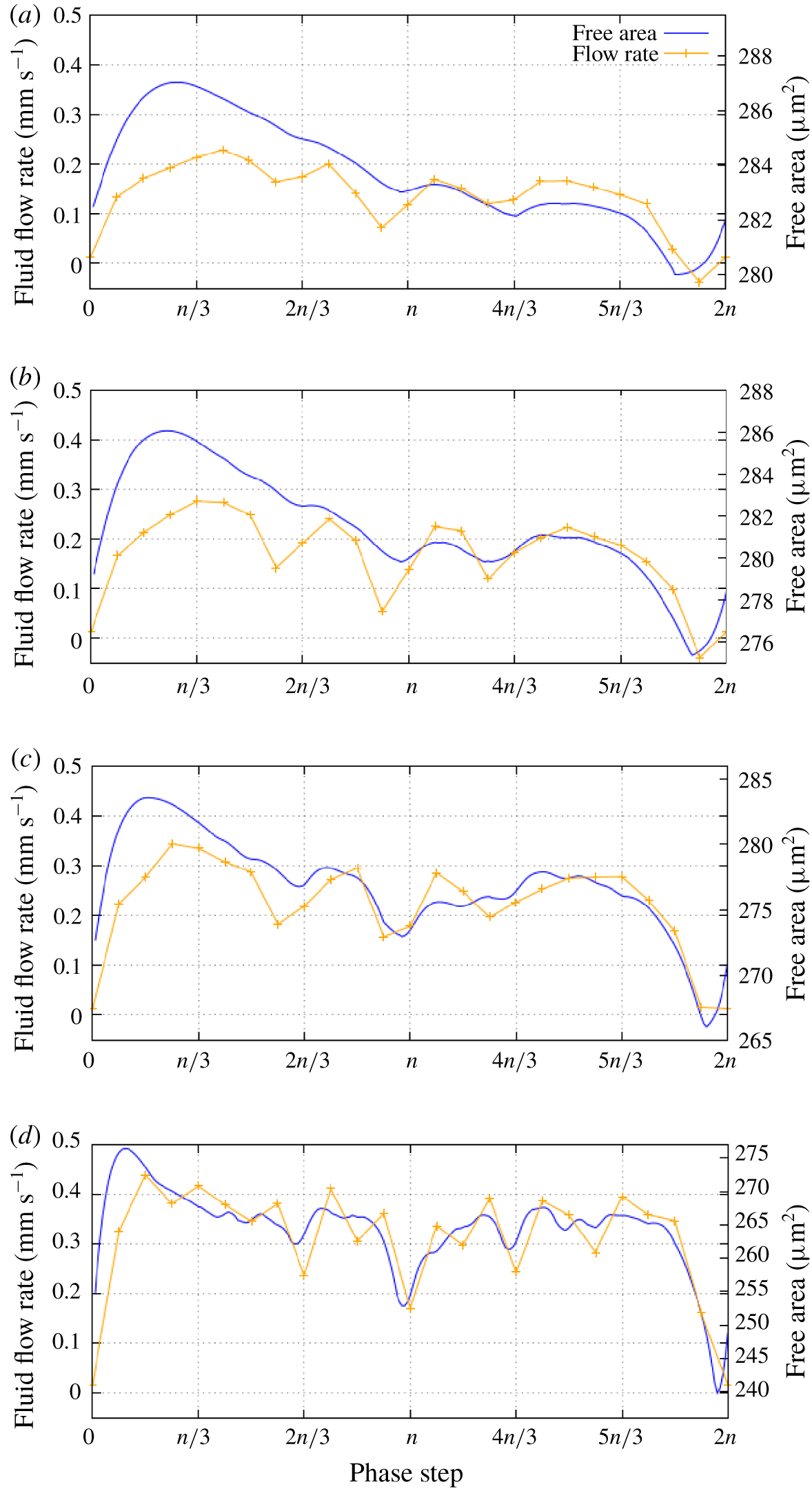
A direct comparison of the free area calculated from our analytical model and the fluid flow rate generated by our simulations showing a strong correlation between the two for a range of cilium spacing values (a)  $3.0~\unicode[STIX]{x03BC}\text{m}$; (b)
 $2.25~\unicode[STIX]{x03BC}\text{m}$; (c)
 $1.5~\unicode[STIX]{x03BC}\text{m}$; (d)
 $0.75~\unicode[STIX]{x03BC}\text{m}$.

Our equation for free area represents a very specific relationship between free area and phase step, similar to the relationship that we have observed between fluid flow rate and phase step. By comparing the two as in figure 12(a) we can see that there is a direct correlation between free area and flow rate.
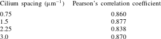
Since free area is also dependent on cilium spacing we have run further simulations to determine how the relationship between flow rate and phase step varies for different cilium spacing. We observed that the correlation between flow rate and free area holds for different cilium spacing, as shown in figure 12(d). A Pearson correlation analysis returns a consistently high correlation coefficient for a range of cilium spacing values, showing that the correlation between free area and flow rate is not only strong but also independent of cilium spacing. Full results from this analysis are included in appendix B. This implies that the variation of flow rate in the numerical model is largely due to the geometric properties of the cilium array, since our free area model does not factor in any complex hydrodynamic effects. We also observe that the optimal metachronal wavelength given by our simulations and our analytical model ( $\unicode[STIX]{x1D706}_{M}\approx 9~\unicode[STIX]{x03BC}\text{m}$) is within the range of metachronal wavelengths observed in vitro (Gheber & Priel Reference Gheber and Priel1997).
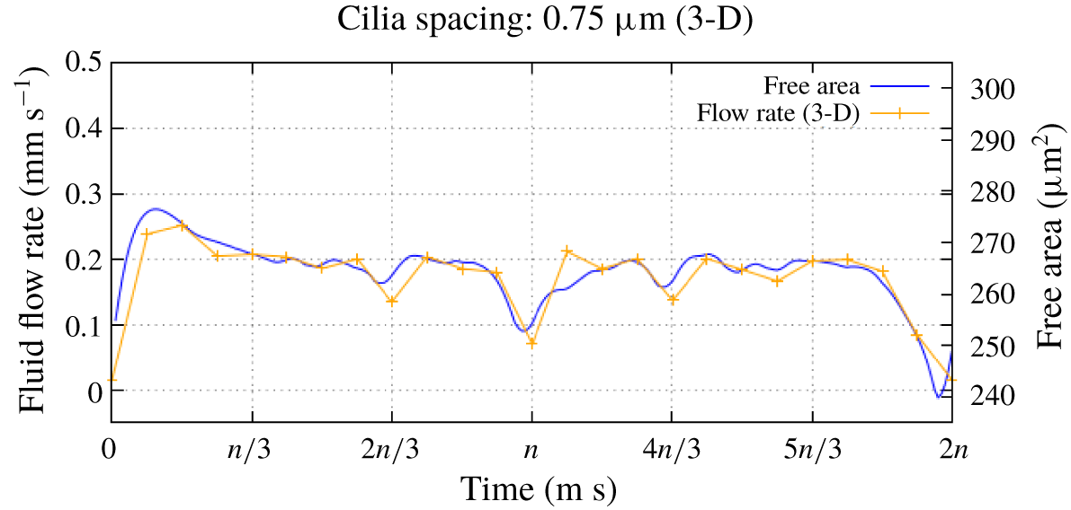
Comparing our analytical model with results from 3-D simulations shows that the variation of fluid flow rate with phase step is almost identical, although the flow rate in the 3-D case is consistently lower as discussed previously. This confirms that the behaviour that we have observed is not caused by the 2-D fluid. We can also see in figure 13 that the correlation between free area and flow rate still holds for the 3-D case.
Free area and flow rate in 3-D model shows the same correlation as the 2-D model.

From the results in figures 12 and 13 we can see that while there is a clear link between free area and flow rate, the data also imply that there is an amount of free area that does not contribute to the fluid flow. This is because only fluid that is above the cilium array will flow consistently, and the fluid that surrounds the cilium array will flow back and forth as the cilia beat. It is clear from our analytical results that the free area in the lower fluid region is vital for effective fluid flow although the fluid in this region does not necessarily contribute to the net fluid flow.
Our simulation results generally show that the lowest values for fluid flow rate correspond with synchronised beating. Local minima in fluid flow rate are also associated with phase step values that correspond with partial synchrony, where a cilium in the array is synchronised with another nearby cilium. For example when  $\unicode[STIX]{x0394}\unicode[STIX]{x1D719}=\unicode[STIX]{x03C0}$ cilium
 $n$ is synchronised with cilium
 $n\pm 2$, and when
 $\unicode[STIX]{x0394}\unicode[STIX]{x1D719}=2\unicode[STIX]{x03C0}/3$,
 $4\unicode[STIX]{x03C0}/3$ cilium
 $n$ is synchronised with cilium
 $n\pm 3$. However, there are some cases where these minima are offset from synchrony and the lowest values of fluid flow rate correspond with symplectic metachrony. A good example of this occurs when the cilium spacing is
 $2.25~\unicode[STIX]{x03BC}\text{m}$ as in figure 12(b). Similar behaviour has been observed by Ding et al. (Reference Ding, Nawroth, McFall-Ngai and Kanso2014). We propose that this behaviour is due to the minimal free area that is associated with symplectic metachrony which reduces the effectiveness of the active stroke to the point where the recovery stroke is actually more effective at driving fluid flow, as predicted by our analytical model.
6 Conclusions
We have conducted a number of simulations using our immersed boundary lattice Boltzmann model in order to identify how the metachronal wavelength of a beating cilium array affects the rate of fluid flow. Based on the results of these simulations we have derived a simple analytical model of the cilium array to determine the free area of fluid that is available to each cilium as it beats, and how this value depends on the metachronal wavelength. By comparing our analytical model with our simulation results we have determined that there is a strong correlation between free area and fluid flow rate, which supports the validity of our analytical model.
Both our analytical and simulation results indicate that an antiplectic metachronal wave ( $\unicode[STIX]{x0394}\unicode[STIX]{x1D719}<\unicode[STIX]{x03C0}$) is more effective at generating fluid flow than a symplectic wave (
 $\unicode[STIX]{x0394}\unicode[STIX]{x1D719}>\unicode[STIX]{x03C0}$), which agrees with other simulations (Khaderi et al. Reference Khaderi, den Toonder and Onck2011; Chateau et al. Reference Chateau, Favier, D’Ortona and Poncet2017). Our simulation results also show that symplectic metachrony can be even less effective at generating fluid flow than synchronised beating, in agreement with Ding et al. (Reference Ding, Nawroth, McFall-Ngai and Kanso2014). Using our analytical model we can attribute this behaviour to the cilia having a greater amount of free area during the recovery stroke and effectively working against the active stroke to produce fluid flow in the opposite direction.
Acknowledgements
This work was funded by the University of Sheffield. We would like to thank Dr R. Hawkins for all of her support, and Dr P. Richmond for his help with optimising our model.
Declaration of interests
The authors report no conflict of interest.
Appendix A. Fluid region testing
In our parametric study we have taken advantage of the periodic boundaries in our model to minimise the simulation runtimes. The model is able to generate a continuous metachronal wave in the cilium array as long as the  $x$ dimension contains a whole number of metachronal wavelengths. During the parametric study we changed the
 $x$ dimension of the model so that the runtime of each simulation is as small as possible, and we have conducted a set of simulations to confirm that this has a minimal effect on the results of the simulations.
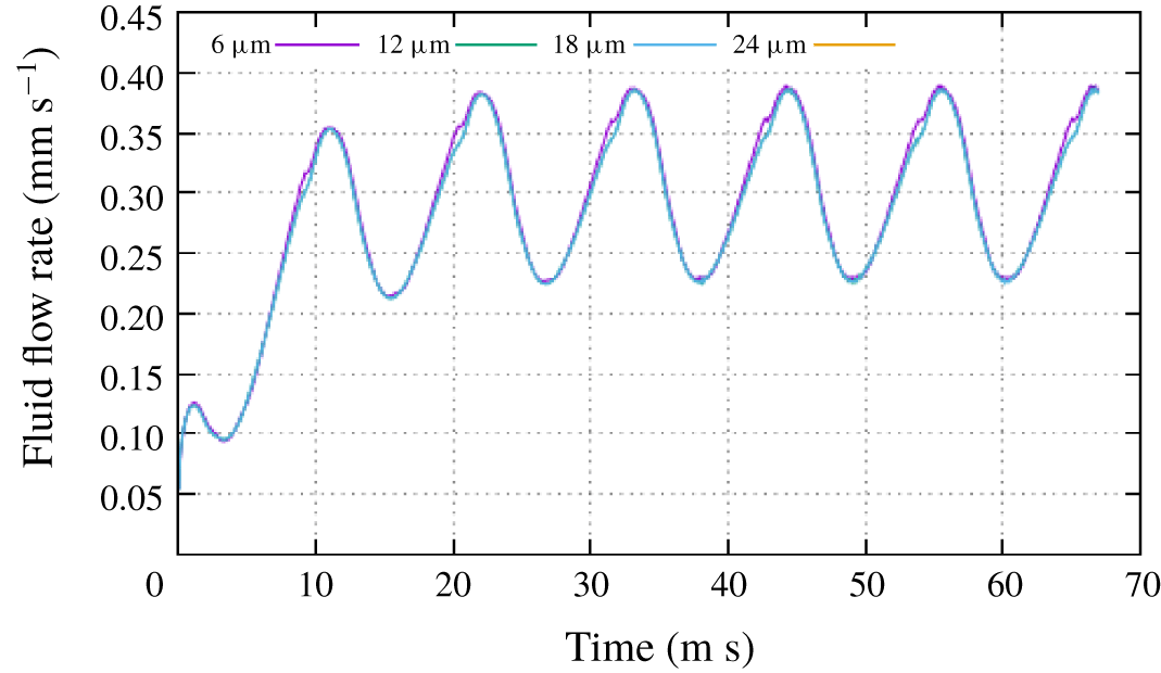
Results from different fluid region sizes with the same metachronal wavelength and cilium spacing. Showing minimal variation of flow behaviour when the  $x$ dimension of the fluid region is increased.

Figure 14 shows results from four simulations that were run with the same phase step  $(\unicode[STIX]{x0394}\unicode[STIX]{x1D719}=\unicode[STIX]{x03C0}/3)$ and cilium spacing
 $(S=2~\unicode[STIX]{x03BC}\text{m})$. Each simulation has a different
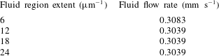
 $x$ dimension, and our results confirm that the fluid flow behaviour for each simulation is virtually identical. Further analysis of these results show that the fluid flow rate is also virtually unaffected by the variation of the
 $x$ dimension as shown in table 2.
Fluid flow rate for different fluid region sizes.

Appendix B. Pearson’s correlation
We have confirmed the observed correlation between our simulation results and our analytical model numerically using the Pearson’s correlation coefficient  $(r)$. By calculating
 $r$ for each different cilium spacing using the equation
 $$\begin{eqnarray}r=\frac{N\sum XY-(\sum X\sum Y)}{\sqrt{[N\sum X^{2}-(\sum X)^{2}][N\sum Y^{2}-(\sum Y)^{2}]}},\end{eqnarray}$$
where  $N=24$ data points,
 $X$ represents the fluid flow rate from our simulation and
 $Y$ represents the fluid flow rate from our analytical model. With this equation can investigate how strong the correlation between our analytical model and simulation results, and whether this correlation depends on cilium spacing.
Pearson’s correlation analysis.

The results in table 3 show that there is a consistent positive correlation between our analytical model and simulation results, confirming our initial observations.