The study of financial factors in economic growth and development is an area of increasing interest, and a well-developed literature indicates that finance plays a first-order and enduring role (Levine Reference Levine1997, Reference Levine, Aghion and Durlauf2005). And though economic historians are typically more circumspect in attributing too much to financial factors, a growing body of evidence suggests that improvements in finance served to transform the U.S. economy from a state of disarray, confusion, and stagnation in the 1780s into a more modern and growing economy in subsequent decades (Rousseau and Sylla Reference Rousseau and Sylla2005). Similar experiences in England, the Netherlands, and Japan add weight to these arguments.
Nevertheless, to infer from this evidence that finance was an exogenous driver of growth is as simple as it is incorrect, and begs the question of what put these virtuous cycles of finance and development into motion? In the United States, it took rising state debts, the risk of potential defaults, and the inefficiencies of multiple currency systems to bring about a sea change in financial policy under Treasury Secretary Alexander Hamilton. But beneath these issues, the new financial structures arose in response to the nation's seemingly unlimited potential for generating real economic returns.
A half-century after the Federal Constitution, with the nation's sovereignty secure and its financial institutions already at work in the Eastern population centers, a network of banks rapidly formed in the Midwest. The network effectively filled in gaps in the geographic distribution of financial services as Midwestern customers no longer needed to travel to the region's largest city to bank. What caused the expansion? Hugh Rockoff (Reference Rockoff1974) and Arthur Rolnick and Warren Weber (1984) argue that lowered barriers to entry from the free banking movement were central. These undoubtedly contributed to the expansion, but the choice of where to locate a new bank was likely determined by the expected profitability of different sites. Specifically, we argue that the burgeoning rail system provided the real-sector catalyst that directed and accelerated the expansion of banking into specific locations of the Midwest. While we do not mean to suggest that banking networks would not have eventually formed without the rails, we argue that the banking map and the implied distribution of capital would have looked quite different without the railroad.
While Robert Fogel (Reference Fogel1964) disputed and ultimately rejected the proposition that railroads were indispensable for national economic development, railroads were the key transportation development of the nineteenth century and, from the very first, linked established markets. And though banks and financial services were already available in these markets, unsettled areas along the new rail routes immediately became more attractive prospects for development, and increasingly so as railroads pushed further westward towards the frontier. More nimble and dense than canals, railroads opened trading networks between the frontier and major population centers. Indeed, this is central to recent work by David Donaldson and Richard Hornbeck (2012). Here, we ask a more specific question: Did the economic potential created by the rails determine where banks would set up shop to finance a wave of new economic activity? We believe the answer is yes. It is clear that isolated banks without some form of organized and improved transportation could do little to influence the course of trade. However, the interaction between the two over the period from 1836 to 1861 turns out to be crucial.
Because of the availability of complementary databases, we focus upon the antebellum Midwest. Specifically we look at the expansion of railroads and banks in seven midwestern states: Illinois, Indiana, Iowa, Michigan, Missouri, Ohio, and Wisconsin, which achieved statehood between 1803 (Ohio) and 1848 (Wisconsin). For each state, we have detailed annual information about the spread of the transportation network and the location of each bank that opened (or closed) prior to 1862. Our emphasis upon the railroad rather than agriculture or manufacturing as the driving force behind bank location reflects the tremendous potential for trade and development that these railroads enabled. Jeremy Atack and Robert Margo (2011) and Atack, Fred Bateman, Michael Haines, and Margo (2010) relate the coming of the railroad to increases in agricultural productivity, market specialization, land values, urbanization, and manufacturing factories. Was this then what lay behind the spread of financial intermediaries? And did these intermediaries finance the local improvements that made communities along the path of the railroad successful? We cannot answer these questions directly since finance would have continued to develop without railroads, but rather we address it indirectly by testing whether banks entered quickly after their county received a railroad rather than later after growth had begun.
Our evidence tells a two-part story. First, railroads were laid out to link existing centers of finance and commerce. Early charter banks tended to have high capital stocks and were concentrated in large population centers. Seeing the opportunity to expand and diversify their local economy, early bank owners often helped fund the first rails. For instance, the Baltimore and Ohio Railroad was not only initially recommended by a group headed by the president of the Mechanics Bank of Baltimore, but its stock was also issued by that bank along with the Farmers’ Branch Bank in Frederick and the Hagerstown Bank in Hagerstown (Stover Reference Stover1987). Even when they did not directly fund the rails, existing banks provided information and facilitated transactions for the railroad companies. The existing banking system, therefore, influenced the anchors of the railroad network.
Second, once the rails were laid, additional banks sprang up along the tracks. While the railroad's main terminals were often located in financial centers, the connecting lines ran through many previously undeveloped areas in between. Indeed, most new banks during the period entered just a year or two after the railroad came through their county and, in some cases, freshly chartered railroad companies also took out banking charters to help raise capital. For example, in 1834 promoters Sherman Stevens and Alfred Williams secured a bank charter from the Michigan Territory to build the Detroit and Pontiac Railroad Company to connect Detroit to the rich agricultural land of Oakland County to the northwest of the city. Finding adequate finance for that venture, however, proved difficult so these same promoters persuaded the territorial legislature to charter the Bank of Pontiac the following year (Burton et al. Reference Burton, Burton, Blue and Miller1930). That same year, the promoters of the Erie and Kalamazoo Railroad also secured a banking charter for a bank in Adrian, Michigan, which would be the western terminus of the railroad (Anonymous 1882, p. 918). It is in this sense that the rapid development of rails during the antebellum period may be responsible for filling out the banking map more rapidly than would have otherwise occurred.
ANTEBELLUM BANKS AND TRANSPORTATION
The early American banking system was the product of state-level legislative activities that created a loose collection of rules with inconsistent standards across time and jurisdictions. Before 1837, approval of any bank's charter depended as much on political influence as on financial resources.Footnote 1 The slow entry of banks led to an intense desire for liquidity in developing areas and demands for change.
Midwest state legislatures responded by passing a series of measures now known as “Free Banking Laws.” Starting with Michigan in 1837 and continuing through Iowa in 1858, these laws replaced individual legislative charters for banks with a well-defined set of capital, reserve, and note issue requirements but otherwise free entry. While specific requirements varied across states, most laws allowed speedy entry with relatively small startup costs, and ultimately every Midwest state except Missouri adopted some form of free banking.Footnote 2 Thus, relative to early charter banks, which often experienced delays in the entry process and were forced to dissipate potential rents to acquire or protect their charters, free banks could obtain charters quickly and therefore respond more quickly to economic opportunities. Regardless of charter type, however, antebellum banks generated most of their profits from the spread between their borrowing and lending rates. We should therefore expect banks to be established in areas with newly emerging economic opportunities in need of financing and few competitors supplying it.
Due to high travel costs and a primitive road network, individuals and businesses were for the most part forced to bank locally. This likely made population density the most important determinant for bank entry because high-density areas provided a concentrated pool of depositors and loan applicants. Moreover, because borrowers could generally not borrow from distant banks where they were unknown, there was little possibility of direct interest rate arbitrage, allowing those banks to exploit their monopoly power.
Areas connected to a transportation network would also have been attractive to banks.Footnote 3 Transportation networks concentrated people and economic activity into specific areas. Atack, Bateman, Haines, and Margo (Reference Atack, Bateman, Haines and Margo2010) find that the arrival of a railroad increased the fraction of people living in an urban area in the Midwest by more than 50 percent.Footnote 4 At the same time, manufacturing plants, with their need for physical and working capital, also located around railroads and waterways to take advantage of lower shipping costs (Atack, Haines, and Margo Reference Atack, Haines, Margo, Rhode, Rosenbloom and Weiman2011). A location with a railroad could thus be attractive to potential bankers regardless of its current population.
At the same time, locations with incumbent banks would generally have been less attractive for new banks. Richard Sylla (Reference Sylla1969), John James (Reference James1976), and Richard Sullivan (Reference Sullivan, Atack and Neal2007) show that increased bank competition during the late 1800s was necessary to lower interest rates on loans. By entering a developing area first, a bank could keep loan rates high and deposit rates low. This incentivized banks to enter an area early in the development process and before other banks arrived. For example, an individual might preemptively open a bank in an area that would soon get a railroad, trading off low initial profits for higher future profits.Footnote 5
While banks were attracted to urban areas, we focus on their attraction to rails and other transportation for a variety of reasons. First, the arrival of a railroad was often the underlying cause of rapid urbanization, and if we were to focus solely on population in such cases we could confound accelerations in population growth with the arrival of a railroad. Second, while early railroads were likely constructed to connect existing financial and commercial centers, those built later were generally exogenous to the entry of new banks.Footnote 6 Ports and rivers were largely predetermined by nature, whereas the routes of railroads, while not entirely unconstrained by geography, were planned in advance and represented a product of conscious and deliberate choice whose construction took time.Footnote 7 Therefore, the decision to build a railroad between two cities was made using initial information, and the timing of the rail's arrival was a function of the distance and topography between it and the railroad's starting point.
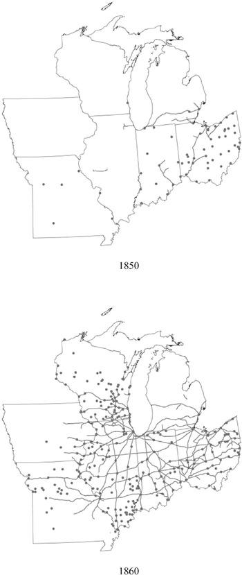
Figure 1 illustrates the high correlation between banks and railroads. In both 1850 and 1860, most railroads started or ended where a bank was located, and the majority of banks were located somewhere along a railroad. The critical question, however, is when did those banks and railroads enter relative to each other? Knowledge of this timing will help sort out the determinants of location choice for both banks and rails. Before testing the relative timing of bank and railroad entry, we describe our data on each and examine their growth individually. We then illustrate how the two co-evolved.
A FIRST LOOK AT THE DATA
Sources and Methods
Although previous studies (Callender Reference Callender1902) have suggested a connection between banks and transportation, we are able to examine the timing of the two events by assembling a comprehensive database containing annual information on every Midwest bank and the extent of the transportation network prior to the Civil War. These, in turn, are linked to economic and demographic data from the decennial censuses for 1840, 1850, and 1860.
The Location of Banks and Railroads in 1850 and 1860

The transportation data come from GIS databases developed by Atack from a variety of contemporary and retrospective sources including digitized maps, reports by various government agencies, compilations from travel guides, and the like (Atack Reference Atack2013) that have been geo-referenced against county boundary files from the Minnesota Population Center National Historical Geographic Information System (2011) project. In particular, the basic Midwest rail data are from Frederic Paxson (Reference Paxson1914), who used contemporary travel guides for Ohio, Indiana, Illinois, Michigan, and Wisconsin and news accounts from Henry Varnum Poor's American Railroad Journal (1832) to draw a series of maps detailing the spread of the rail network in the Old Northwest between 1848 and 1860.Footnote 8 These data are supplemented with digitized maps for Iowa and Wisconsin from the David Rumsey map collection and extended to 1861 using maps created by George Rogers Taylor and Irene Neu (Reference Taylor and Neu1956). The exact location of the individual rail lines was determined so far as possible using a number of different strategies: where rail lines run today, where satellite imagery indicates that ground was disturbed, and from topographical maps that show cuts and fill and often bear notations such as “old railroad grade” in the general vicinity of where Paxson reports a rail line to be located.
Data on canals are from Carter Goodrich (Reference Goodrich1961), supplemented by nineteenth century sources such as Poor (Reference Poor1970) and various histories of the individual canal systems that provide dates on when specific sections of canals were opened to traffic, e.g., Noble Whitford (Reference Whitford1906). Data regarding the extent of steam navigation on the western rivers are from Louis Hunter (Reference Hunter1949) and various U.S. government reports, especially those of the War Department, which was responsible for the Corp of Engineers.
We use these GIS databases to construct a county-level panel from 1836 to 1861 with variables such as the number of railway miles in a county and indicators for whether the county had a port, river, or canal within its boundaries. We then link these transportation measures to county-level census data assembled by Haines (Reference Atack, Bateman, Haines and Margo2010), which updates the original Inter-University Consortium for Political and Social Research (ICPSR) database (1979).
The county, then, is our basic unit of observation. However, as everyone who has ever worked with these data for nineteenth century America knows, many county boundaries changed from decade to decade, especially those closer to the frontier of settlement where the creation of local governments was an on-going process. While the geocoded data accommodate such changes, one cannot simply link the Census data by county across time because of these boundary changes. There are several possible solutions. One approach is to restrict the analysis to those counties with constant boundaries over the time period using sources such as William Thorndale and William Dollarhide (Reference Thorndale and Dollarhide1987) and ICPSR (1979) estimates of the area of each county. This procedure, however, leaves out large swathes of the region, much of it on the northern and western edges, but also large areas of central Illinois, northwestern, central, and southeastern Ohio, and the northern two-thirds of Michigan. Another approach, used by Hornbeck (Reference Hornbeck2010), is to start from the assumption that population and economic activities were uniformly distributed within counties and then reallocate those attributes proportionately as the geographic area within political boundaries changed.
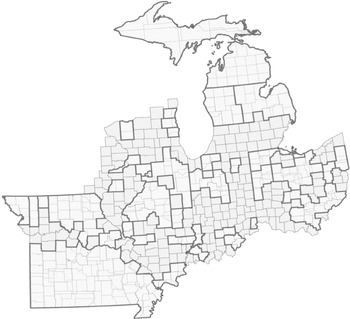
We have adopted a different, GIS-based procedure with the goal of identifying specific geographic areas for which we can also obtain consistent economic and demographic information using the Minnesota Population Center NHGIS (2011) county boundary files.Footnote 9 In 1840, the seven Midwestern states that we consider were divided into 388 “counties,” some of which were unattached (that is to say were not formally a part of any county) and some of which extended well beyond the seven states’ western and northern boundaries.Footnote 10 We began by eliminating those western and northern areas in Iowa and Wisconsin whose 1840 boundaries extended beyond those of the modern states. We also had to “trim back” some counties in Iowa and Wisconsin until we could locate a determinate western and northern boundary within these states for our analysis. That resulting area, shown by the outline in Figure 2, embraced 351 counties in 1840 and 503 counties by 1860, of which 220 were identical according to GIS (meaning that they shared the same geographic space and had identical geometries) in 1840, 1850, and 1860.
The area covered by the remaining, non-GIS identical counties (embracing what were 131 counties in 1840 and which became 283 counties in 1860) can, however, be combined at the county level within the fixed state borders into identical contiguous areas comprised of complete individual counties in each year. Since these “aggregated counties” represent a constant geographic area for which consistent economic and demographic data can be assembled from the censuses, they too are a part of our panel.Footnote 11 These are shown in Figure 2 and are bounded by the heavier outline. Within each, the lighter lines show the 1840 and 1860 boundaries of the counties that are aggregated into these “super-counties.”
“Counties” in the Midwestern Sample (1837–1861)

We link these “county”-level census data (i.e., identical counties plus the aggregated “super counties”) and our GIS transportation databases to Warren Weber's (2005) enumeration of antebellum banks. Weber's census of banks has been geocoded and extended to the outbreak of the Civil War using annual editions of the Merchants and Bankers’ Almanac (Merchant and Bankers’ Almanac, s.d.), which provide a comprehensive list of U.S. banks in each year (Jaremski Reference Jaremski2010).Footnote 12 We have also made a few adjustments to Weber's data based on these directory listings and other contemporaneous information. In particular, the changes involved merging banks that “closed” in one year with those that “opened” almost immediately after with the same name. We believe that these reflect charter renewals or mergers so that the “new” bank was not necessarily an entering bank. However, while these few changes affect the timing of the second or third bank in a county, they do not change the date at which a county gained its first bank.
New Banks by Year and States (1830–1860)

Timing of Bank Entry
Figure 3 shows three primary waves of Midwest bank entry. The first took place between 1833 and 1839. Of the 103 banks that started up during this period, three-fourths were in Michigan and Ohio and the rest were in Indiana. This entry wave was quickly ended by Panics of 1837 and 1839, which led to the closing of a large number of Michigan free banks and discouraged further bank creation.Footnote 13 It was not until the panics subsided and many states had defaulted on their debts that a second wave of bank entry occurred from 1845 to 1848. Once again, 49 of the wave's 51 new banks started in Michigan and Ohio, suggesting that the wave was particular to conditions in these specific states. The third wave of bank entry began around 1850 and lasted through the start of the Civil War. Unlike the previous ones, this wave spread banks through the remaining Midwest states, with banks entering Indiana and Illinois during the early 1850s, Wisconsin during the mid-1850s, and Iowa or Missouri during the late 1850s.
The few years with abnormally high entry rates correspond with aggregate price fluctuations or changes in bank regulatory regimes, especially those affecting bank capital. For instance, more than 100 banks entered during 1852 and 1853 after the passage of free banking laws in Indiana and Illinois. Further, the large number of banks entering Illinois and Wisconsin during 1858 and 1859 seem to have been the result of free banks taking advantage of declines in the prices of southern bonds that could be used to back their note circulations (Dwyer and Hasan Reference Dwyer and Hasan2007; Economopoulos Reference Economopoulos1988).
The composition of banks also changed over time. In the earliest period, many Midwest banks were, at least partly, state-funded and subject to state direction. For example, the State Bank of Indiana system, which started in 1834 and grew to more than 20 branches (Indiana 1838), derived half of its capital from that state. The State Bank of Ohio system was started in the 1840s and expanded to more than 40 branches (White Reference White1902). The branches operated independently of the main office and one another but were subject to mutual oversight and collective responsibility for the obligations of other branches (Indiana 1838; White Reference White1902). More importantly for this study, both of the enabling laws stipulated the general geographic regions in which the branches were to locate but not the exact locations. These banks were particularly large and concentrated in large cities. The few other banks chartered prior to free banking tended to be politically connected and were often created to help float the states’ internal improvement bonds. Over time, and often with the advent of free banking, newly entering banks were able to avoid political entanglements. The resulting banks were generally smaller and located in rural areas. Therefore, while early banks might have been able to fund railroads, later banks would not have been able to contribute directly to the expansion of the railroad system.
Timing of Canal and Railroad Entry
According to Harvey Segal (Reference Segal and Goodrich1961), there were three waves of canal construction, each beginning in a spirit of hope and optimism and ending in collapse and panic. The first were concentrated in New York and Pennsylvania and sparked by the optimism generated by the immediate and resounding success of the Erie Canal. This phase ended with the realization that the topography of Pennsylvania would prevent that state's ambitious canal system from duplicating the Erie's success.Footnote 14 The second canal construction phase saw canals expand into the Midwest, sparked by ambitious plans and generous support in Ohio to link the Ohio River and the Great Lakes together at multiple points along the breadth of the state. The second canal boom, however, collapsed when the Panic of 1837 disrupted the construction of the (overly ambitious) Wabash and Erie Canal and also railroad projects like the Detroit and Pontiac Railroad.Footnote 15 The third canal phase saw much less ambitious plans for feeder canals to expand the market reach of the existing system and to bolster the technical viability of the trunk canals.
While Ohio was the first Midwest state to invest in canals, it was not the first to adopt rail technology. Indeed, Ohio early on tried to discourage competition from rails in a failed effort to prevent the devaluation of its canals (and their revenue)—many of which had been built with public funds. Instead, the first rail service in the region started in Michigan even though it had not yet obtained statehood. The territorial legislature chartered the Pontiac and Detroit Railroad in 1830Footnote 16 and the Erie and Kalamazoo Railroad in 1833 (Dunbar Reference Dunbar1969; Meints Reference Meints2005). Seeing Michigan's success, Ohio relented in its opposition and began railroad construction in 1835. By 1837, Ohio's Mad River and Lake Erie Railroad began operation from Sandusky (on Lake Erie) to Bellevue.
Despite early railroad successes in Ohio and Michigan, other western rail construction did not take off for a decade and a half. For instance, there were still very few railroads in the other Midwest states even as late as 1848, and most were relatively short-routes that did not connect to the eastern rail system. The first ran from Indianapolis to the Ohio River at Madison, whereas the others were short Illinois lines (Springfield to the Illinois River at Beardstown, and Chicago to Elgin). The Midwest states did not begin to construct an interconnected system of railroads until the 1850s, but once underway, expansion proceeded rapidly. Nationwide, approximately 22,000 miles of track were laid over the decade, and much of it was built in the Midwest.Footnote 17 Rails eventually reached across the entire Midwest and connected to the eastern railroad system—Chicago, for example, had an all-rail link to the East Coast by 1858 (Cronon Reference Cronon1991; Grossman, Keating, and Reiff Reference Grossman, Keating and Reiff2004). However, not every county in the region received a railroad, and about 20 percent of Midwest counties still did not have a railroad in 1860.
Our results suggest that the tremendous acceleration of railroad construction during the 1850s was driven more by real-side factors than by banking. As seen in the previous section, the banking system was relatively slow to recover from the Panics of 1837 and 1839, and while the surviving large banks likely continued to fund railroads, the few new entering banks were too small to fund such large-scale railroad projects. Instead, the rise in the demand for grain is likely one of the main factors for bringing more investment into the system. This is best seen in the switch from small regional railroads to an interconnected network and the growth of feeder railroads running from North to South.
Matching Banks and Transportation
Transportation and banks likely have a symbiotic relationship. Just as banks did not open in undeveloped locations, investors did not build railroads to nowhere. In this way, the existing Midwest banks might have helped define the terminal stations of the railroad system, whereas new banks might have taken advantage of locations in-between that had been newly opened to trade. In this section, we examine these relationships by asking three empirical questions: (1) Did railroads match up with existing financial centers? (2) Were new banks more likely to enter those places connected to transportation networks? And, (3) when did banks enter relative to an area's first railroad?
Fraction of Counties with Railroad (1837–1861)

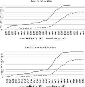
To observe the influence of existing banks on rail growth, we separated the counties based on whether or not they had at least one bank in 1836. Figure 4 graphs the fraction of counties in each group that had a railroad over time. Most of the early railroads were located in counties with banks and the trend continued in the 1840s and 1850s. By the late 1850s, every county that had a bank in 1836 also had a railroad, yet only 70 percent of those counties without a bank by 1836 had a railroad within their borders. While we still must control for factors such as population density and general economic activity, the raw data suggest that existing banks helped map out the rail network.
Midwest Banks Near Transportation Networks at Date of Entry

Notes:
The table presents the percentage of entering banks that were within the defined distance from a transportation network. Banks are sorted into the different decade groups based on their year of entry. Distances are straightline distances from points to polylines calculated by GIS.
Source:
Weber (Reference Weber2005) and Jaremski (Reference Jaremski2010).
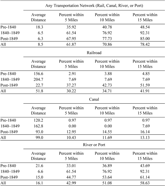
We measure the effect of all improved modes of transportation on bank creation by examining the average distance between entering banks and the nearest railroad, canal, and river/port. The data show a distinct shift in the choice of bank location with respect to transportation and the different improved means of transportation (Table 1). A few early banks were located along rivers and ports, but most others were far from transportation, likely a result of the lack of options. However, those banks entering after 1840, when railroads and canals were more prevalent, located only 6.5 miles away from the nearest “modern” transportation medium. Later bank entry seems to have corresponded more to railroads than canals. Indeed, even at the height of canal construction, nearly three times as many banks were established within 5 miles of a railroad than within 5 miles of a canal. This difference could be the result of the increased speed and more direct routes offered by railroads relative to canals, which greatly improved conditions for personal travel.
We observe the timing of bank entry relative to the entry of a county's first railroad in Figure 5. Few banks entered a county before it received a railroad, and over two-thirds entered afterward. Specifically, most banks entered a year or two after a railroad. For example, only 12 banks entered the year before a rail arrived, 26 entered the same year that the railroad arrived, and 38 entered the year after. Because the presence of a bank in a county might have delayed the entry of a second bank, counting the total number of bank entries could overstate the extent to which banks followed the railways. Yet even when we only count a county's first bank, the number that enter a year after a railroad (10 banks) still exceeds the number that entered the year before a railroad (5 banks) or at the same time as a railroad (7 banks).
The lower panel of Figure 5 illustrates what happens when we remove those counties with a port on one of the Great Lakes from the sample. Because both ports and railroads were valued for their ability to create trade, banks might have been willing to enter counties with ports even if they did not have a railroad. Therefore, mixing counties with and without ports could positively bias the number of banks that entered before a railroad. As expected, when port counties are removed, the number of banks entering before a railroad decreases from 26 to 23 but those entering after the railroad only fall from 38 to 37. Banks thus seem to have been primarily attracted to the first transportation network entering a county, rather than railroads per se.
ECONOMETRIC ANALYSIS
The raw data suggest that railroads were built to link large commercial and financial centers, while new banks sprung up quickly once the rail was laid. Our descriptive analysis, however, is unable to control for other important factors. For instance, railroads might have been attracted to more densely populated areas rather than banks, and the late arrival of banks in specific states might reflect the absence of a Free Banking Law to facilitate bank entry. We therefore proceed with a multivariate regression approach.
Number of Banks Entering Relative to Year of Railroad Entry (1837–1861)

Our transportation and bank data are annual. However, the census data are only decadal, so we cannot simultaneously control for county-level characteristics and compare the annual expansion of banks and railroads. Consequently, we break up the analysis into two steps. We first examine whether county characteristics reduce the correlation between banks and rails at the county level through a decennial analysis for 1840–1860 that considers both the effect of the initial number of banks on railroad growth and the effect of railroads on subsequent bank growth. Next, we examine the specific timing of bank entry relative to railroads and free banking laws by explaining annual changes in each variable. By isolating the number of banks that entered directly before or after a railroad, we are better able to determine whether the construction of a railroad in a particular location was the main determinant of bank entry rather than the population and economic activity that was to follow.
Determinants of Rail Entry by Decade
Before examining the response of bank entry to the growing rail system, we test whether the initial presence of a bank encouraged railroad expansion. We examine the arrival of a railroad and growth in the number of railroad miles using an ordinary least squares (OLS) regression where each observation is a county-decade.Footnote 18 The dependent variable is the change in railroads in county i during the decade d, and the main explanatory variable is the number of banks present in the county at the start of that decade.Footnote 19 Since a county can only gain a railroad once, we drop counties that already had a railroad at the beginning of the decade (d – 10) and estimate the regression separately for the 1840s and the 1850s. The regression model is:

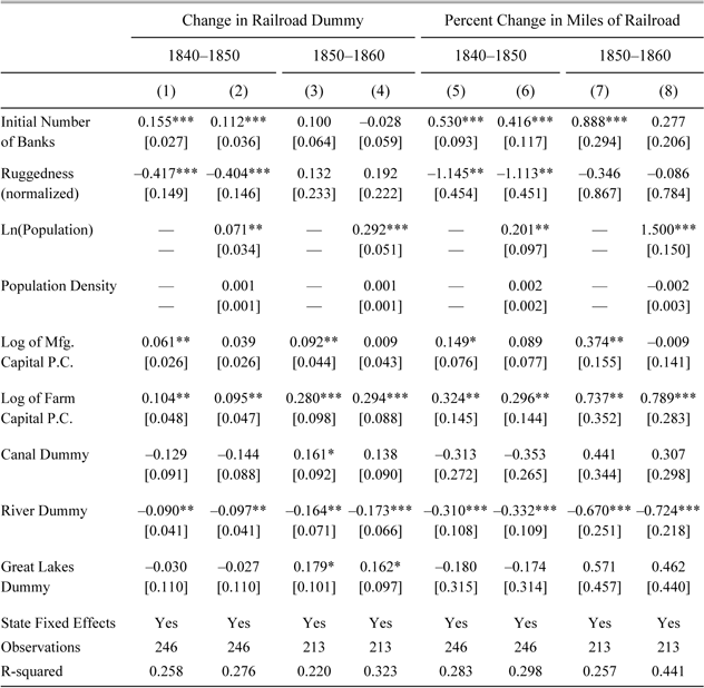
where Ri measures the average ruggedness of the county's terrain, Xi,d is a vector of county-level control variables, SS denotes fixed effects for states, and ei,d is the error term. The county-level controls include the logarithms of manufacturing capital per capita, farm capital per capita, and population, along with population density and dummy variables representing whether the county had a canal, a navigable river, or was on the Great Lakes.Footnote 20 Proposed by Shawn Riley (Reference Riley, Degloria and Elliot1999), our index of terrain ruggedness measures the change in elevation from a digital elevation model derived from satellite imagery between neighboring cells, each 90 meters by 90 meters in a 3 × 3 matrix, averaged across each “county” and normalized across the seven states so that the most rugged county has an index of 1.Footnote 21 This ruggedness metric has the advantage of not varying over time. It is also unlikely to be correlated with bank entry but should have been a significant deterrent to rail construction by raising both construction and operating costs. Because the presence of a bank has been related to increases in population, we estimate the regression model with and without population and population density on the right hand side.Footnote 22
The coefficient on the number of banks is generally positive and statistically significant in Table 2. For each additional bank in a county, the probability of getting a railroad increased by at least 11 percent in the 1840s but by less in the 1850s when the coefficient on this variable is estimated with less precision and population growth seems to have been more important. Ruggedness was a significant impediment to railroad construction in the 1840s when construction was concentrated along the Ohio River in the hills of southern Indiana and southern Ohio. Its impact in the 1850s, on the other hand, was minimal since construction by then was advancing across the flat prairies.
Overall, we interpret the results as indicating that the initial banking system helped provide some structure to the growing railroad network. This seems to be most true during the early years when the railroad's foundations were being laid rather than later years when the gaps in the rail network were being filled.Footnote 23
Existing Banks' Effects on Railroad Entry (1840–1860) (Ordinary Least Squares Estimates)

* = Significant at the 10 percent level.
** = Significant at the 5 percent level.
*** = Significant at the 1 percent level.
Notes:
The dependent variables are changes in the rail variable over a decade. The dummy is the change from zero to one and the miles of railroad is the percentage change (starting from one mile). As there would be no change in the railroad dummy, we exclude counties that had a railroad at the beginning of the period. All money values are deflated to 1860 dollars using Officer (2008). Terrain ruggedness is measured using the “terrain ruggedness index” developed by Riley (Reference Riley, Degloria and Elliot1999). This metric is based on the sum of changes in elevation for a 3×3 matrix of 90 meter by 90 meters cells, averaged across each county, and normalized for the seven Midwestern states. Robust standard errors appear in brackets beneath the coefficients.
Sources:
Bank data: Weber (Reference Weber2005) and Jaremski (Reference Jaremski2010). County-level economic and demographic data: Haines and ICPSR (Reference Haines2010). GIS locational data: Atack (Reference Atack2013). See also text.
Determinants of Bank Entry by Decade
We begin to analyze the banking system's response to railroads using a similar structure to the previous section. Each observation is a county-decade, and the dependent variable is the number of banks that entered county i during the decade d. As before, we exclude observations for counties that already had a railroad at the start of the decade, and estimate the equation separately for each decade.Footnote 24 Given that every county starts without a railroad, the approach is similar to a difference-in-difference model, and by controlling for contemporaneous county-level variables rather than initial values we tend to bias the effect of railroads downward. The specification is:

where FBYrsi,d is the number of years a free banking law was in place.Footnote 25 Once again we estimate the regression with and without population and population density.Footnote 26
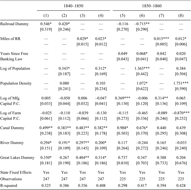
The results reported in Table 3 show that the arrival of new rails encouraged bank entry. A county that received a new railroad in the 1840s could expect to gain an extra 0.42 to 0.55 banks over the decade. Alternatively, a county with no railroad in 1840 would generally need to have built between 35 and 44 miles of track within its borders to add one bank to the county. This relatively minor amount of railroad construction would have matched the average number of entering banks per county (0.91) during the decade.
The coefficients on miles of railroad remain positive and significant during the 1850s, but the railroad dummy becomes significantly negative when population density and the log of county population are included. This seems to be driven by the large number of rural counties that received only a few miles of railroad over the period. For example, defining the railroad dummy as 18 more or miles of track rather than any track at all, is sufficient to render the coefficient on the modified dummy always positive and statistically significant.
Free banking laws allowed relatively rapid entry without the need for legislative approval, but while positive, the coefficient on the number of years with free banking installed in the decade is not generally statistically significant. This is likely due to the fact that many free banks entered a year or two after a law was passed rather than over the entire decade.
Table 3 also indicates that non-rail transportation was particularly important for bank growth during the 1840s but less so during the 1850s. For instance, a county that was on a navigable river was expected to gain between 0.19 and 0.30 more banks during the 1840s when river trade was especially vibrant (Haites, Mak, and Walton Reference Haites, Mak and Walton1975; Hunter Reference Hunter1949), but saw little or no change—and perhaps even shrinkage in the number of banks—during the 1850s. Similarly, counties on the Great Lakes could expect to gain between 0.27 and 0.40 banks in the 1840s but the coefficients for these counties in the 1850s are not statistically significant. The only transportation method that seems to hold up over time is canals, whose impact on the number of banks rivals that of the railroad, but even then, it is not significant when included in a regression with railroad miles in the 1850s. The results suggest that the rail system largely replaced existing transportation networks and might have made use of some canal ways.Footnote 27 Indeed, rails (especially early on) followed river valleys.
The Impact of New Railroads on Bank Entry (1840–1860) (Ordinary Least Squares Estimates)

* = Significant at the 10 percent level.
** = Significant at the 5 percent level.
*** = Significant at the 1 percent level.
Notes:
The dependent variable is expressed as the number of banks that entered the county during the specified decade. Counties with railroads at the start of the decade are excluded. The railroad dummy denotes counties that had a railroad at any time during the decade. All money values are deflated to 1860 dollars using Officer (2008). Robust standard errors appear in brackets beneath the coefficients.
Source:
Bank data: Weber (Reference Weber2005) and Jaremski (Reference Jaremski2010). County-level economic and demographic data: Haines and ICPSR (Reference Haines2010). GIS locational data: Atack (Reference Atack2013). See also text.
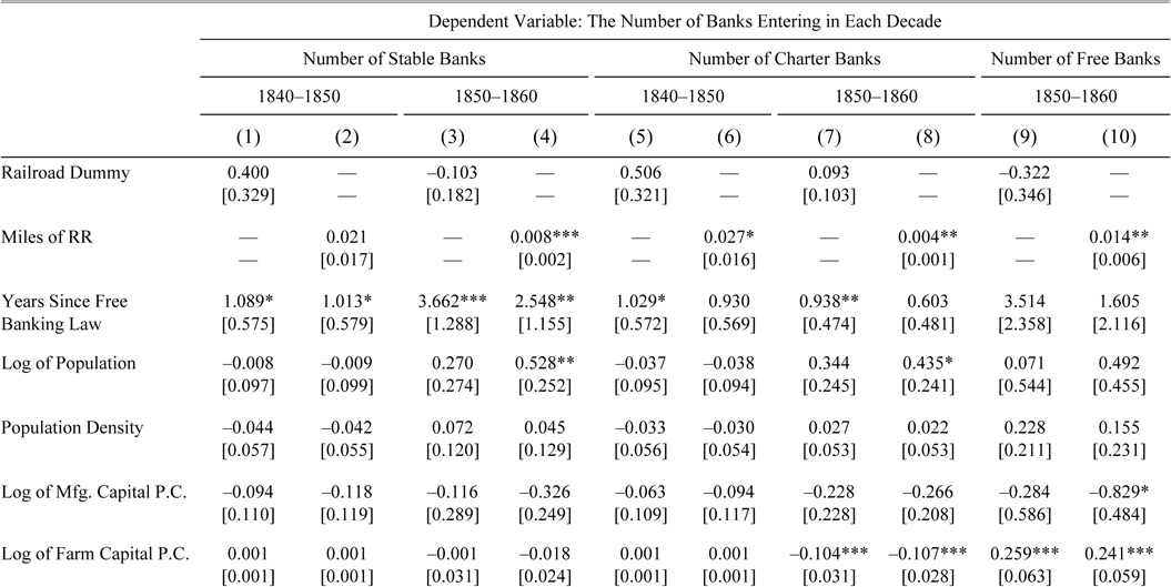
The contemporary literature suggests that some fraudulent banks avoided transportation networks. As these wildcat banks would generally reduce the effect of a railroad on bank entry, we re-estimate the regressions using a dependent variable that only counts the entry of banks that remained in operation for three or more years, which we define as “stable banks.”Footnote 28 This restriction should eliminate those banks that intended to defraud their customers or that did not take steps to diversify their asset portfolios properly. Seen in Table 4, the coefficients on the railroad variables increase relative to the average number of entering stable banks (0.57) but lose some of their statistical significance in the 1840s. A county that gained 25 miles of railroad could expect to gain a statistically insignificant 0.53 stable banks in the 1840s and 0.20 stable banks in the 1850s. The negative coefficient on the railroad dummy is also no longer statistically significant. Stable banks thus seem to have been attracted to areas with railroads.Footnote 29
We also report separate regressions for free and charter bank entry in Table 4 to account for their different start-up procedures. The number of railroad miles is correlated with entry of both free and charter banks. A county that went from having no railroad in 1850 to having 25 miles of railroad in 1860 could expect to gain 0.10 charter banks and 0.35 free banks by the end of the decade. Relative to the mean number of new charter banks (0.26) and of new free banks (0.65) in a county, the results are economically significant. The results also show that, if anything, the negative and statistically significant effect of the railroad dummy in Table 3 is driven by free banks during the 1850s.
Determinants of Bank Entry by Year (1837–1861)
In the previous sections, we established links between railroads and banks at the decadal level for the 1840s and 1850s. We now turn to annual data from 1837 through 1861 to establish more firmly the timing of bank entry relative to a railroad. The dependent variable is the number of banks that entered county i in year t. We use a dummy variable for whether the county gained a railroad during a given year and the percentage change in railroad miles (rather than the level) for two reasons. First, the approach avoids confounding slow population growth (or other county-level factors) with the sudden entry of railroads. While railroads were likely to have increased the growth of population, it was likely to have taken a few years. Second, the approach identifies the immediate effect of railroad entry on banks rather an effect commencing years later. For instance, the change in the railroad dummy will only take a value of unity in one period, meaning if it did not have an immediate effect on banks then our models would not pick it up. We also include the previous and forward change in the railroad variable to further pinpoint the timing of bank entry. The regression is:

where ui is a vector of county-level fixed effects and the other controls retain their previous definitions. The use of annual data allows us to include fixed effects for counties that may account for other omitted yet unobservable characteristics at the county level.Footnote 30
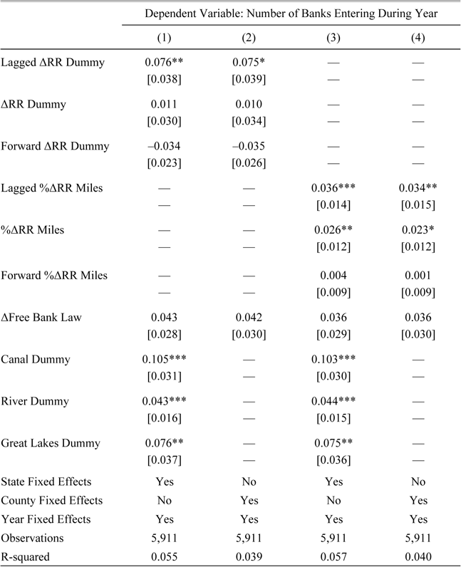
The timing of railroad entry was important (Table 5). A county that gained a railroad would expect to gain 0.011 additional banks in that year and 0.076 additional banks in the year after, with the latter representing a doubling of the number of new banks over the average of all counties (0.08). Counties receiving a bank were also less likely to see a railroad follow in the next year, though the coefficients (−0.34 and −0.35) in columns (1) and (2) of Table 5 are not statistically significant. The coefficients on the contemporaneous and lagged changes in railroad miles are also statistically significant, though the coefficients on the “leads” are not.
Once again we find that water transportation attracted banks. A county with a river or a canal could expect to gain 0.043 and 0.105 more banks per year respectively, and one located along one of the Great Lakes gained 0.076 more banks per year. It is important to note, however, that these variables are essentially county-fixed effects. Therefore, the significant coefficients suggest that the transportation methods made it more likely that a bank would enter a county but do not say much about when that entry was likely to occur. When we account for the timing of counties that gained a canal after 1837, we do not find a contemporaneous correlation between it and bank entry.
The Impact of New Railroads on Bank Entry by Type (1840–1860) (Ordinary Least Squares Estimates)


* = Significant at the 10 percent level.
** = Significant at the 5 percent level.
*** = Significant at the 1 percent level.
Notes:
The dependent variables are the number of stable, free or charter banks that entered the county during each decade. Stable banks are defined as those that remained in operation for three or more years. Counties with railroads at the beginning of the decade are excluded. States without a free banking law are dropped from the free banking regressions. The railroad dummy denotes counties that had a railroad at any time during the decade. All money values are deflated to 1860 dollars using Officer (2008). Robust standard errors appear in brackets beneath the coefficients.
Sources:
Bank data: Weber (Reference Weber2005) and Jaremski (Reference Jaremski2010). County-level economic and demographic data: Haines and ICPSR (Reference Haines2010). GIS locational data: Atack (Reference Atack2013). See also text.
The Impact of Railroads on Annual Bank Entry (1837–1861) (Ordinary Least Squares Estimates)

* = Significant at the 10 percent level.
** = Significant at the 5 percent level.
*** = Significant at the 1 percent level.
Notes:
The dependent variables are the number of banks that entered the county during each year. The change in the railroad dummy denotes counties that had their first tracks laid in a given year. All money values are deflated to 1860 dollars using Officer (2008). Robust standard errors appear in brackets beneath the coefficients.
Sources:
Bank data: Weber (Reference Weber2005) and Jaremski (Reference Jaremski2010). County-level economic and demographic data: Haines and ICPSR (Reference Haines2010). GIS locational data: Atack (Reference Atack2013). See also text.
Regression Coefficient on Railroad Measures for Various Leads and Lags

Effects of railroads on bank entry by type of bank (1837–1861)


* = Significant at the 10 percent level.
** = Significant at the 5 percent level.
*** = Significant at the 1 percent level.
Notes:
The dependent variables are the number of banks that entered the county in each year. Stable banks are defined as those that remained in operation for three or more years. The change in the railroad dummy denotes counties that had their first tracks laid in a given year. All money values are deflated to 1860 dollars using Officer (2008). Robust standard errors appear in brackets beneath the coefficients.
Sources:
Bank data: Weber (Reference Weber2005) and Jaremski (Reference Jaremski2010). County-level economic and demographic data: Haines and ICPSR (Reference Haines2010). GIS locational data: Atack (Reference Atack2013). See also text.
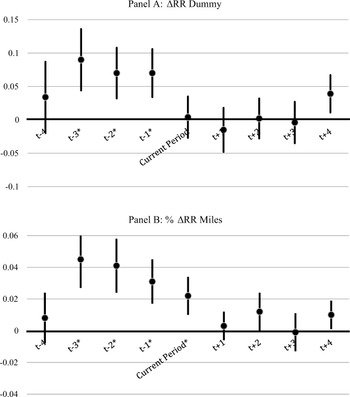
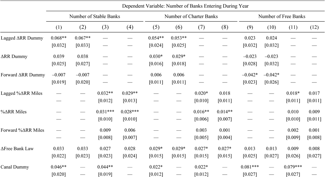
Moreover, restricting consideration to just a one-year lead or lag in the variable, as in Table 5, does not bias our results. Figure 6 presents the railroad coefficient (and standard errors thereof) for leads and lags of 0, 1, 2, 3, and 4 years. The coefficient on each leading variable is not statistically significant and is very close to zero. On the other hand, banks are significantly more likely to enter a county one to three years after a railroad ran through it. We also performed two robustness checks on the data (Table 6). First, we replaced the dependent variable with the number of entering banks that survived three or more years to remove fraudulent banks. These longer-lived banks, once again, have the strongest connection to rails. For instance, a county that gained a railroad could expect to gain 0.039 more stable banks that year, and 0.068 banks in the year following. Second, we separated the regressions by bank type to see whether the different chartering processes affected the entry decisions of banks. They appeared to matter: using railroad miles as the explanatory variable, charter banks moved into an area just after it got a railroad or at the same time, whereas free banks were much less likely to enter a county in the year before a railroad but tended to enter a county in the year after a railroad was built.
Tightening the Geographic Unit
The previous panel regression identified the effect of railroads on new bank entry at the county-level to control for traditional boundaries and state regulation. However, these counties differ considerably in size. Even without the aggregation of those counties whose boundaries changed into “super-counties” with constant external geographic borders, Midwest counties in 1860 varied in size by a factor of 7.5, from just 165 square miles to 1,238 square miles. Such variations increase the likelihood that larger counties will have specific features or attributes—for example, a bank or a railroad—that smaller counties might lack even if these features or attributes were randomly distributed, thereby biasing our associations among these features.
One solution is to examine the joint association of features in arbitrarily distributed but identically sized areas that exhaust the space but not overlap one another. Borrowing from urban economics, we filled the area covered by the sample with hexagons, each ten miles across from side-to-side, using an ArcGIS user-written script.Footnote 31 This generated a “fishnet” or “beehive” of 3,542 hexagons, each with an area of 86.6 square miles or about one-half the area of the smallest county in the Midwest.
The approach allows us to more closely match railroad and bank locations; however, it still has some limitations. First, some hexagons extend (slightly) beyond the boundaries of the seven states or include bodies of water.Footnote 32 For instance, in Figure 7, we see that several hexagons contain little to no land at all. Second, the global positioning coordinates for the locations of banks are somewhat noisy. Because we do not have the street addresses of each bank, we have instead placed banks at the center of the town in which they are located and set their geographic coordinates accordingly. Therefore, those banks that are located on the border of a hexagon might very well lie on the other side of that border. As a result, we might expect more banks to enter just before a rail arrives.
Hexagon Sample (1837–1861)

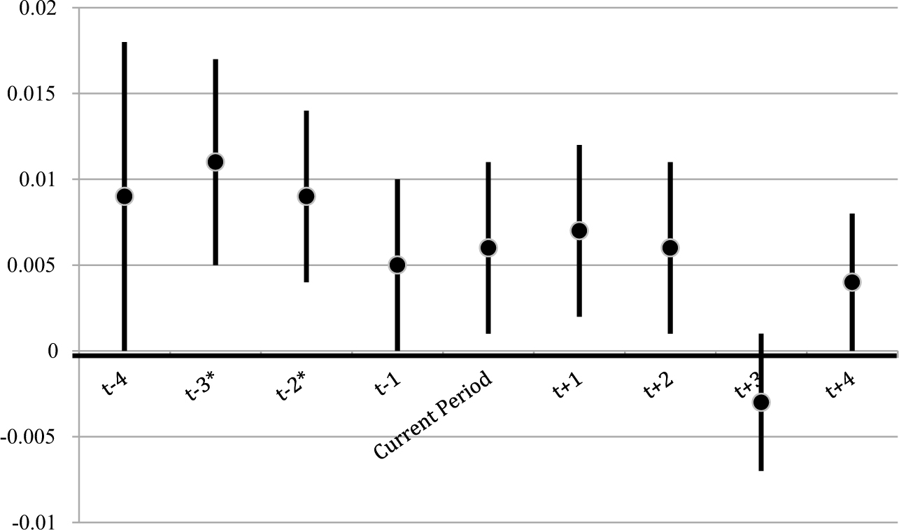
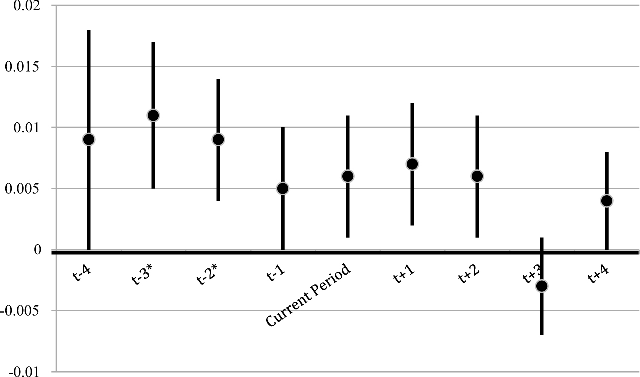
Because of the limited geographic area of each hexagon, we concentrate on the change in the railroad dummy rather than the percent change in railroad miles. Moreover, as many hexagons span two different states, we cannot include the free bank dummy. The model, therefore, includes hexagon fixed effects to capture the other transportation methods and any other time invariant characteristics. Figure 8 contains the coefficients on the change in the railroad miles for various leads and lags. While the coefficients on the leading variables are larger than they were for the cross-country sample, only lags of two and three years are statistically significant. These data thus confirm that new banks sprung up along the railroads rather than somewhere else.
Regression Coefficient on Railroad Dummy For Various Leads and Lags Using Hexagon Map
DECOMPOSING RAILROADS BY TRACK ORIENTATION (1837–1861)
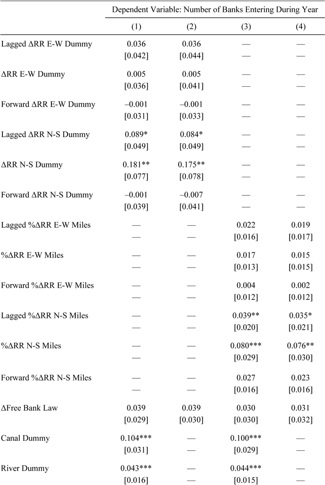
The previous sections have shown that existing banks helped lay the foundation for the railroad network, whereas new banks quickly sprouted up along the new routes. So far, however, we have not addressed what aspect of railroads attracted those banks. In this section, we attempt to understand the decision of banks by separating railroads into those whose track ran North-South versus East-West. Railroads that ran East-West were longer, denser, and carried both freight and passengers potentially to East Coast financial and commercial centers. North-South railroads were generally shorter and carried goods to and from the large cities on the Great Lakes and large rivers such as the Mississippi and Ohio. Therefore, if banks were attracted to areas with a strong potential for gaining population, we would expect them to locate primarily along East-West railroads. However, if banks were interested in facilitating trade with the South, we would expect them to locate primarily along North-South railroads. We test these hypotheses by splitting the railroad variables in models (2) and (3) based on their dominant orientation.Footnote 33
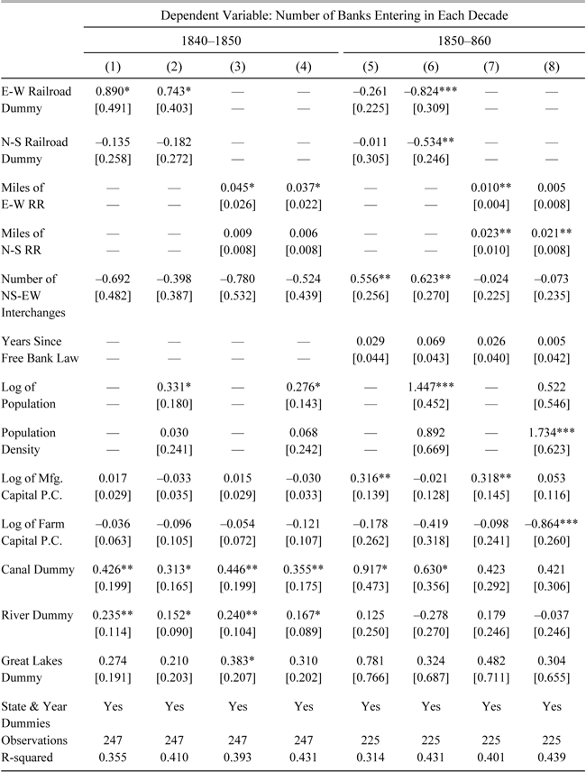
Table 7 shows that early banks might have been attracted to East-West railroads, but later ones were also drawn to North-South routes. During the 1840s, the coefficients on both East-West railroad variables are statistically and economically significant, whereas the coefficients on both North-South railroad variables are not. A county that gained 25 miles of East-West railroad during the 1840s could expect to gain 1.125 new banks, while a county gaining 25 miles of North-South railroad could expect to gain only an insignificant 0.225 banks. During the 1850s, however, 25 East-West miles would lead to only 0.25 more banks whereas 25 North-South miles would lead to 0.575 more banks. The differing results are likely due to the different types of banks that entered in each decade. During the 1840s, only charter banks could be created, and due to the more stringent and burdensome requirements placed on them by state legislatures, might have needed more immediate access to a larger population base to be deemed likely to succeed. However, the passage of free banking laws allowed new banks to issue large numbers of notes with relatively little capital, and thus free banks might have been more inclined to locate in rural areas albeit ones with trading options.
By estimating equation (3), we can further sort through the decision-making of banks. In Table 8, we see that North-South railroads are the most closely associated with the timing of bank entry. The lagged and contemporaneous coefficients on both the North-South railroad dummy and miles are generally statistically and economically significant, while no coefficients on the East-West railroad variables are significant. Once again this is likely due to the effect of free banks rather than charter banks, as free banks were better equipped to enter quickly after railroads.
The data thus suggest that banks, especially later entrants, were attracting railroads because of their opening of trading routes. These small banks could provide trade credit and working capital to farmers and manufacturers that were shipping their goods down the Mississippi or up the Great Lakes.
Decomposing Railroads by Direction of Track (1840–1860) (Ordinary Least Squares Estimates)

* = Significant at the 10 percent level.
** = Significant at the 5 percent level.
*** = Significant at the 1 percent level.
Notes:
The dependent variables are the number of banks that entered the county in each decade. The railroad dummies denote counties that had a railroad of that type at any time during the decade. All money values are deflated to 1860 dollars using Officer (2008). Robust standard errors appear in brackets beneath the coefficients.
Sources:
Bank data: Weber (Reference Weber2005) and Jaremski (Reference Jaremski2010). County-level economic and demographic data: Haines and ICPSR (Reference Haines2010). GIS locational data: Atack (Reference Atack2013). See also text.
Panel OLS — Decomposing Railroads by Track Direction (1837–1861)

* = Significant at the 10 percent level.
** = Significant at the 5 percent level.
*** = Significant at the 1 percent level.
Notes:
The dependent variables are the number of banks that entered the county in each year. The change in the railroad dummy denotes counties that had their first tracks laid in a given year. All money values are deflated to 1860 dollars using Officer (2008). Robust standard errors appear in brackets beneath the coefficients.
Sources:
Bank data: Weber (Reference Weber2005) and Jaremski (Reference Jaremski2010). County-level economic and demographic data: Haines and ICPSR (Reference Haines2010). GIS locational data: Atack (Reference Atack2013). See also text.
CONCLUSION
The stories of American industrialization often have banks and railroads at their heart. However, these two factors have most often been studied separately rather than together. We show that the two are not separate entities but rather were intimately connected, and that their relationship evolved over time.
Banks and bankers played a central role in the initial spread of rail transportation. For instance, at the very start of the railroad age on February 19, 1827, about two dozen of Baltimore's leading citizens gathered at the home of George Brown, a partner with his father in the banking firm of Alexander Brown and Son, to hear the report of a committee chaired by Philip Thomas, the president of the Mechanics Bank. The committee was charged with addressing the question of how Baltimore should respond to the commercial challenges posed to the city by New York's Erie Canal and Philadelphia's Main Line canal, but instead of recommending the construction of a canal, they recommended the construction of a railroad across the Allegheny Mountains to the Ohio River and the Baltimore and Ohio Railroad was quickly formed. The newly chartered railroad opened its subscription books to the public from March 20, 1827 through March 31 at the Mechanics Bank in Baltimore, the Farmers’ Branch Bank in Frederick, and the Hagerstown Bank in Hagerstown (Stover Reference Stover1987).
As this recounting of the origins of the B&O Railroad shows, banks and bankers played a central and critical pioneering role: finance clearly led the process (Bordo and Rousseau Reference Bordo and Rousseau2012; Rousseau and Sylla Reference Rousseau and Sylla2005; Rousseau and Wachtel Reference Rousseau and Wachtel1998). And while the leadership of these large eastern financiers over successor institutions was largely preordained, we find that large banks in the Midwest also helped form the anchors of the region's railroad network.
In a few locations, banks and railroads went hand-in-hand. We have already described how the Michigan Territorial Legislature in 1835 chartered the Erie and Kalamazoo Bank in Adrian as an adjunct to the railroad of the same name and the Bank of Pontiac as a side venture of the Detroit and Pontiac Railroad. Another historian of the period remarked that “Strange as it may now seem to us, the combination of a railroad and a bank was no new proposition” before going on to describe the passage of “An Act to incorporate the Macomb and Saginaw Railroad Company and for other purposes”—the principal of which turned out to be the establishment of a bank in Mt. Clemens under the corporate name “The President, Directors and Company of the Bank of Macomb County,” speculating that the popularity of railroad projects was such that any related bank stood to benefit, just days before Michigan became a state (1882, pp. 918–9).
Over time, the transportation revolution, and railroads in particular, opened up opportunities for new banks. The arrival of a railroad brought with it the potential for commercial development and cross-country trade to locations along the new route. New banks quickly moved in to take advantage of these opportunities. We find that nearly half of the new Midwest banks that entered after 1840 opened within a few years of a railroad's arrival in their county.
The financial system and its banks not only funded the initial expansion of railroads, but also helped to improve business conditions by following the railroads into undeveloped lands where new communities and older hamlets became vibrant centers of local activity. Railroads arrived at a time when economic activity and population growth were particularly vigorous, and in the midst of the nation's first wave of corporate capitalism. They, along with the banks that came with them, proceeded to break the pattern of economic fragmentation that hampered regional integration more quickly than would have been possible otherwise, and rendered the links from financial factors to real activity established early in the nation's history stronger and even more secure.
Appendix – Coding Railroad Orientation and Interchanges
Railroad Directions

Rail lines were classified as “East-West (EW)” or “North-South (NS)” (mutually exclusive) based upon whether the dominant orientation of the line (not just in the vicinity of a specific location) was to points east and west or north and south. Thus, for example, the Illinois Central is classified as a NS railroad whereas the Ohio and Mississippi Rail Road (which runs from Cincinnati to St. Louis) was EW. Similarly, the Pittsburgh, Fort Wayne, and Chicago Railway is classified as EW although it runs NW from Pittsburgh to Fort Wayne. The breakdown is shown in Figure A.1. The few railroads that could have been classified either way were branch lines and they have been classified according to the orientation of the more major line to which they connected.
Points where EW and NS lines intersect have been tagged (as points) and coded with the earliest date at which it became possible to switch from an EW line to a NS line. Note that this date is simply the earliest date at which it was possible to switch from railroads headed in one direction to an orthogonal direction. This was not necessarily the earliest date at which one had the choice to travel in both orthogonal directions. Reality, of course, is more complicated. Indianapolis, for example has four distinct EW-NS intersections within 2.5 miles of one another with dates 1851, 1852, 1852, and 1853. Moreover, Sidney, Ohio has an EW railroad entering from the east in 1853 and leaving to points further west in 1854 and a NS railroad entering from the south in 1857 and leaving northwards in 1859. It, of course, is classified as having an EW-NS interchange from 1857.
Whenever possible, railroad lines that were very close together but did not touch were included as interchanges. For instance, the GIS network shows the Greenville & Miami Railroad (built 1852) intersecting with the Columbus, Piqua, and Indiana Railroad (built 1859) just outside Union City but within a couple of hundred feet of the Bellefontaine and Indiana Railroad (built 1854) to which it does not (seemingly) connect directly. At the same time, care was taken to leave out railroads that were very close together but had a geographic impediment between them. For instance, railroads running on opposite sides of the Mississippi River are close, but the ferry across the river was probably expensive and almost certainly risky and time consuming.