1 Introduction
Graph classification and decomposition problems are central topics in discrete mathematics and theoretical computer science, with deep connections to algorithm design, computational complexity and combinatorial optimization [Reference Bondy and Murty10, Reference Garey and Johnson22]. Nondeterministic polynomial time (NP) is the class of decision problems solvable in polynomial time by a nondeterministic Turing machine, or equivalently, whose solutions can be verified in polynomial time. A problem is NP-hard if every problem in NP can be reduced to it in polynomial time. Many graph problems of interest are NP-hard, rendering exact algorithms intractable at scale and motivating learned heuristics as a tractable alternative. As a result, research has historically focused on designing heuristics and approximation algorithms to obtain feasible solutions in practice [Reference Hochba29, Reference Li, Ding, Yang, Sherratt, Park and Wang42]. However, handcrafted heuristics are often labour-intensive to design, may rely on substantial domain expertise and often do not generalize well beyond specific instances [Reference Branke, Nguyen, Pickardt and Zhang11, Reference Liu, Zhang, Tang and Yao49]. This motivates the exploration of learning-based methods as scalable alternatives to manual algorithm engineering.
In recent years, graph neural networks (GNNs) [Reference Kipf and Welling38] have emerged as a powerful framework for representation learning on graphs which enable models to learn task-specific embeddings through message passing and aggregation mechanisms [Reference Gilmer, Schoenholz, Riley, Vinyals and Dahl23, Reference Hamilton28]. GNNs have been extensively studied in graph mining tasks such as node classification, link prediction and graph classification [Reference Liang, Qian, Yu, Griffith and Golmie45, Reference Xia, Sun, Yu, Aziz, Wan, Pan and Liu73]. Beyond this, they have also shown promise in solving combinatorial optimization (CO) problems including graph colouring [Reference Lemos, Prates, Avelar and Lamb41, Reference Schuetz, Brubaker, Zhu and Katzgraber60, Reference Watkins, Montana and Branke69, Reference Zhang, Zhang and Wu78] and the travelling salesman problem [Reference Liang, Wang, Li, Zhou, Zhang and Wang46, Reference Shi and Zhang63, Reference Xing and Tu74]. These highlight the potential of learned heuristics in domains traditionally dominated by algorithm design. The application of learning-based methods to CO problems has grown rapidly in recent years [Reference Bengio, Lodi and Prouvost7, Reference Mazyavkina, Sviridov, Ivanov and Burnaev51, Reference Peng, Choi and Xu54]. Within graph structured CO tasks, two of the most extensively studied problems are the graph colouring problem (GCP) [Reference Formanowicz and Tanaś20] and the travelling salesman problem (TSP) [Reference Jünger, Reinelt and Rinaldi34]. Much of the progress in these areas stems from adapting GNNs to either approximate classical algorithms or serve as learned heuristics.
1.1 Solving GCPs and TSPs with GNNs
Supervised approaches to GCP typically rely on labelled instances generated by exact solvers or handcrafted heuristics. For example, Lemos et al. [Reference Lemos, Prates, Avelar and Lamb41] used a constraint satisfaction problem (CSP) solver to label instances and trained a GNN to answer the decision version of the GCP for a constant
$C$
 . Other works leverage synthetic graphs with known chromatic numbers [Reference Ijaz, Ali, Ali, Laique and Khan33] or incorporate heuristic procedures during training or post-processing [Reference Langedal and Manne40, Reference Zheng, Jin, He, Xue, Zhao, Song and Bian79].
Although these supervised methods often outperform traditional heuristics on graphs of moderate size, they remain fundamentally constrained by the quality and scalability of the labels on which they rely. Exact solvers limit the size of feasible training instances, while heuristic-based labels introduce bias that may restrict generalization. To mitigate these limitations, unsupervised or self-supervised strategies have been proposed, many of which formulate the GCP with physics-inspired approaches. Notably, several methods optimize a relaxation of the Potts model [Reference Wu70], enabling learning without explicit labels [Reference Gao and Hu21, Reference Li, Li, Ma, Chan, Pan and Yu43, Reference Schuetz, Brubaker, Zhu and Katzgraber60, Reference Wang, Yan and Jin68, Reference Zhang, Zhang and Wu78]. Reinforcement learning (RL) methods form a parallel line of work, treating colouring as a sequential decision-making problem and training agents to construct solutions in a sequential manner [Reference Huang, Patwary and Diamos31, Reference Kwon and Kim39, Reference Watkins, Montana and Branke69].
A similar pattern can be observed in research related to the TSP. Supervised frameworks train GNNs on optimal routes produced by exact solvers [Reference Liang, Wang, Li, Zhou, Zhang and Wang46, Reference Prates, Avelar, Lemos, Lamb and Vardi56], whereas hybrid systems augment GNN predictions with classical heuristics or local search procedures [Reference Hudson, Li, Malencia and Prorok32, Reference Min, Bai and Gomes52, Reference Sanyal and Roy59, Reference Xing and Tu74]. Given the extensive body of work on learning-based approaches and GNNs to the TSP, we refer the reader to recent surveys [Reference Alanzi and Menai3, Reference Sui, Ding, Huang, Yu, Liu, Xia, Ding, Xu, Zhang and Yu64, Reference Yang, Wang, He, Wang, Lin, Pan, Wang and Lin76] for further details.
1.2 Other graph related CO problems with GNNs
Beyond GCP and TSP, GNNs have been applied to a wide range of classical NP-hard graph problems, including maximal independent set (MIS), minimum vertex cover (MVC) and maximal clique (MC) [Reference Abe, Xu, Sato and Sugiyama2, Reference Khalil, Dai, Zhang, Dilkina and Song36, Reference Li, Chen and Koltun44]. For a recent survey on GNNs and learning-based methods on graph related CO problems, we refer the interested reader to [Reference Peng, Choi and Xu54]. These studies collectively demonstrate that GNNs can act as strong heuristics, either matching or improving upon traditional optimization methods. Despite this progress, graph decomposition problems remain largely unexplored in the learning-based literature. In particular, to the best of our knowledge, no systematic evaluation of modern GNN architectures has been conducted for locally irregular edge-colouring or related decomposition tasks. We attribute this gap to two factors: (1) the relatively low visibility of these problems compared with standard CO benchmarks such as GCP and TSP; and (2) the absence of publicly available datasets, which hinders reproducibility and limits comparative evaluation.
Although many NP-hard problems are theoretically reducible to one another [Reference Karp35], such reductions often do not preserve the practical structure or difficulty of real instances. This phenomenon is well documented in areas such as SAT [Reference Gomes, Kautz, Sabharwal and Selman24], where instances of equal theoretical complexity can differ in empirical hardness. Consequently, evaluating GNNs on less-studied problem classes provides an opportunity to assess their architectural robustness and adaptability beyond well-established benchmarks. Our work contributes to this direction by examining locally irregular edge-colouring through the lens of graph classification and representation learning.
1.3 GNNs in graph decomposition
Despite this progress, the application of GNNs to graph decomposition problems remains relatively unexplored. A central difficulty lies in the fact that many theoretical graph problems lack inherit node features, while GNNs typically rely on such features to generate embeddings through message passing [Reference Cui, Lu, Li and Yang15, Reference Duong, Hoang, Dang, Nguyen and Aberer16].
One such problem is the locally irregular edge-colouring problem, which asks whether a graph can be decomposed into a set of locally irregular subgraphs using the minimum number of colours [Reference Baudon, Bensmail, Przybyło and Woźniak6]. Not all graphs can be decomposed into locally irregular subgraphs. This gives rise to a natural classification task, where given a graph
$G$
 , one is to determine if
$G$
 is decomposable or exceptional. This problem exhibits strong structural ambiguity, where graphs differing by a single edge may fall into different classes [Reference Baudon, Bensmail, Przybyło and Woźniak6]. This may make it particularly challenging for machine learning models that rely on geometric representations. At the same time, no known efficient algorithm exists for recognizing exceptional graphs, and it is not trivial to classify decomposable and exceptional graphs in general (see Theorem 1).
In this work, we conduct a systematic study of modern GNN architectures on the locally irregular graph classification task. Our contributions are the following.
-
(1) We benchmark multiple popular GNN architectures such as graph convolutional network (GCN) [Reference Kipf and Welling38], GraphSAGE [Reference Hamilton, Ying and Leskovec27], graph attention network (GAT) [Reference Veličkovi’c, Cucurull, Casanova, Romero, Lio and Bengio66] and graph isomorphism network (GIN) [Reference Xu, Hu, Leskovec and Jegelka75] on the task of classifying decomposable and exceptional graphs.
-
(2) To facilitate systematic evaluation, we construct a dataset of 3120 graphs based on theoretical characterizations from [Reference Baudon, Bensmail, Przybyło and Woźniak6] (see Section 3.1), representing the first learning-ready benchmark for this problem, including:
-
• 2600 in-distribution graphs for training and validation;
-
• 520 out-of-distribution (OOD) graphs for robustness evaluation.
-
-
(3) We analyse how different aggregation schemes influence representation quality and generalization.
-
(4) We systematically evaluate the effect of node feature design and perform embedding-space analysis using PCA, t-SNE and clustering metrics to reveal geometric differences among architectures.
Our results highlight substantial performance differences across architectures and demonstrate that feature design plays a critical role in structural graph learning. This work provides evidence that graph decomposition problems can offer a rich and challenging setting for evaluating GNNs beyond traditional benchmarks.
In Section 2, we provide a summary on the locally irregular edge-colouring problem and GNNs. Section 3 details the dataset, experimental setup and aggregation schemes that are used in our study. Section 4 reports and discusses the results obtained from the experiments. Section 5 details the limitations and future directions of this study and finally in Section 6, we conclude the study.
2 Preliminaries
2.1 Locally irregular edge-colouring
Graphs considered in this study are simple and finite unless stated otherwise. A graph
$G$
 with vertex (or node) set
$V$
 and edge set
$E$
 is said to be locally irregular if for every edge
$e \in E$
 , the end vertices of
$e$
 have distinct degrees. A
$k$
 -locally irregular edge decomposition of
$G$
 is analogous to colouring the edges of
$G$
 with
$k$
 colours such that each colour induces a locally irregular subgraph [Reference Baudon, Bensmail, Przybyło and Woźniak6]. This is also known as
$k$
 -locally irregular edge-colouring (
$k$
 -liec). The smallest such
$k$
 for which
$G$
 admits a
$k$
 -liec is called the locally irregular chromatic index, denoted
$\chi _{\mathrm {irr}}'(G)$
 . If
$G$
 admits a locally irregular edge-colouring, we say that
$G$
 is decomposable and
$\chi _{\mathrm {irr}}'(G)$
 is finite. Otherwise,
$G$
 is exceptional and
$\chi _{\mathrm { irr}}'(G) = \infty $
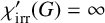 (notation and definitions used in [Reference Bensmail, Merker and Thomassen8]).
Conjecture 1. [Reference Sedlar and Škrekovski62]
(Local Irregularity Conjecture) Every decomposable graph
$G$
 , except for the bow-tie graph
$B$
 , can be edge-coloured using at most three colours such that each colour induces a locally irregular subgraph, that is,
$\chi _{\mathrm {irr}}'(G) \leq 3$
 .
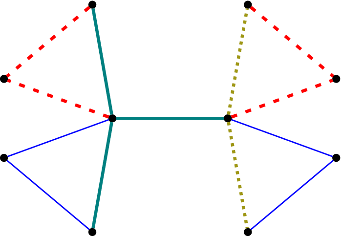
The local irregularity conjecture was first conjectured in 2015 by Baudon et al. [Reference Baudon, Bensmail, Przybyło and Woźniak6]. It was first believed that every decomposable graph required at most 3 colours for a locally irregular edge-colouring. However in 2021, a counter-example to the original conjecture was found (see Figure 1). Then, it was further proved that the bow-tie graph,
$B$
 , is the only counter-example to the original conjecture among all cactus graphs [Reference Sedlar and Škrekovski62]. This has lead to the weaker version of the conjecture (Conjecture 1), where it is currently believed that except for
$B$
 , every decomposable graph required at most 3 colours for a locally irregular edge-colouring.
The bow-tie graph,
$B$
 , and its 4-liec [Reference Sedlar and Škrekovski61].

Here, we will deal with a simpler problem under the umbrella of locally irregular edge-colouring, where given a graph
$G$
 , one aims to classify it as either decomposable or exceptional. The study of locally irregular edge-colouring has traditionally relied on rigorous mathematical proofs, with little to no exploration of machine learning approaches. As a result, the effectiveness of such methods in addressing these problems remains largely unknown.
Theorem 1. [Reference Baudon, Bensmail, Przybyło and Woźniak6]
A connected graph
$G$
 is exceptional if and only if it is: (1) a path of odd length; (2) a cycle of odd length; or (3) a special subclass of cacti,
$\mathfrak {T}$
 .
Theorem 1 lays the foundation to our work, where the complete set of exceptional graphs is characterized. A cactus graph is a graph where any two cycles in the graph shares at most one common vertex. For a node
$v$
 , we let
$\mathcal {N}(v)$
 denote the set of all vertices that are adjacent to
$v$
 . By identifying two vertices
$v_1$
 and
$v_2$
 , we mean the operation that produces a graph in which these two nodes are replaced with a single vertex
$v$
 such that
$v$
 is adjacent to all the vertices in
$\mathcal {N}(v_1) \cup \mathcal {N}(v_2)$
 . The special family of cactus graphs,
$\mathfrak {T}$
 , can be defined inductively as follows [Reference Baudon, Bensmail, Przybyło and Woźniak6]:
-
• the triangle, $K_3$
 is in
$\mathfrak {T}$
;
-
• every other graph of this family may be constructed by taking an auxiliary graph $F$
which might either be a path of even length or a path of odd length with a triangle glued to one of its ends, then choosing a graph
$G \in \mathfrak {T}$
containing a triangle with at least one vertex, say
$v$
, of degree two in
$G$
, and finally identifying
$v$
with a vertex of degree one of
$F$
.


We denote by
$\mathfrak {T}'$
 (notation introduced in [Reference Sedlar and Škrekovski62]) the union of odd-length paths, odd-length cycles and the family
$\mathfrak {T}$
 . Notably, all graphs in
$\mathfrak {T}'$
 are cactus graphs with an odd number of edges. Therefore, cactus graphs represent a significant class in the study of locally irregular edge-colourings, as every known exceptional graph belongs to this category.
2.2 Graph neural networks
Graphs are inherently non-Euclidean structures [Reference Asif4] and lack a fixed topology, which poses challenges for their direct integration into traditional machine learning models. Consequently, it is necessary to employ appropriate techniques that can transform graph data into fixed-size representations, enabling their use within standard machine learning pipelines.
GNNs are a class of neural architectures designed to learn from graph-structured data. Given a graph
$G = (V, E)$
 , where each node
$v \in V$
 is associated with a feature vector
$\mathbf {x}_v \in \mathbb {R}^d$
 , the objective of a GNN is to learn expressive representations that capture both local and global structural information. These representations may correspond to node embeddings
$\mathbf {h}_v \in \mathbb {R}^{d_v}$
 , edge embeddings
$\mathbf {h}_{uv} \in \mathbb {R}^{d_e}$
 or a graph-level embedding
$\mathbf {h}_{G} \in \mathbb {R}^{d_G}$
 , which can then be used for downstream tasks such as node classification, link prediction or graph classification.
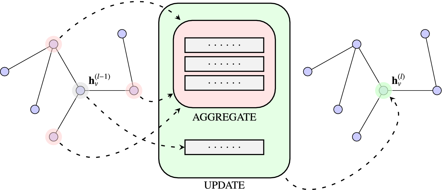
Most GNN models fall under the MPNN framework [Reference Gilmer, Schoenholz, Riley, Vinyals and Dahl23], where node representations are iteratively updated by exchanging information with neighbouring nodes. The message passing process is initialized with the input node features:
$\{\mathbf {h}_v ^{(0)} = \mathbf {x}_v \mid v \in V \}$
 and a fixed number of layers
$L$
 . At each message passing layer
$l = 1,2,\ldots ,L$
 , the embedding
$\mathbf {h}_v^{(l)}$
 of each node
$v \in V$
 is generally obtained through the following steps [Reference Wu, Sun, Zhang, Xie and Cui71]:
-
(1) message aggregation from the local neighbourhood,
$$ \begin{align*} \mathbf{m}_v ^{(l)} = \mathrm{AGGREGATE}^{(l)}(\{\mathbf{h}_u^{(l-1)} \,\vert\, u \in \mathcal{N}(v) \}); \end{align*} $$
-
(2) update of the node embedding using the previous embedding and the aggregated message,
$$ \begin{align*} \mathbf{h}_v ^{(l)} = \mathrm{UPDATE}^{(l)}(\mathbf{h}_v^{(l-1)}, \mathbf{m}_v^{(l)}). \end{align*} $$


Here, AGGREGATE and UPDATE are differentiable and often parametrized functions, enabling end-to-end learning through back-propagation. The AGGREGATE function is required to be permutation-invariant with respect to the unordered set of neighbours
$\mathcal {N}(v)$
 , where typical choices include sum, mean or max pooling. Figure 2 illustrates a single message passing layer for a node, with all nodes updated in parallel using shared AGGREGATE and UPDATE functions.
Illustration of node feature updates in layer
$l$
 of a GNN for a single node.

After
$L$
 layers of message passing, the final node embeddings
$\mathbf {h}_v ^ {(L)}$
 can be used for downstream prediction tasks. For node classification, each
$\mathbf {h}_v ^ {(L)}$
 is passed to a classifier (for example, a multilayer perceptron) with loss back-propagated to update both classifier and GNN parameters. For graph-level tasks, a differentiable, permutation invariant READOUT function aggregates information across all node embeddings to produce a graph-level representation:

This representation is then passed to a classifier and training proceeds similarly. Through iterative message passing, the node embeddings
$\mathbf {h}_v^{(l)}$
 encode information from the
$l$
 -hop neighbourhood of node
$v$
 (all nodes within a distance of at most
$l$
 ), capturing progressively larger structural contexts. In practice, the number of layers
$L$
 is kept relatively small, as deeper GNNs are prone to oversmoothing [Reference Wu, Chen, Wang and Jadbabaie72], where node embeddings become increasingly similar and lose their discriminative capacity. Most GNN architectures follow a common message passing framework, and differ primarily in the specific design of the AGGREGATE and UPDATE functions.
Although there are other methods to automatically obtain node embeddings for graphs such as Deepwalk [Reference Perozzi, Al-Rfou and Skiena55] and node2vec [Reference Grover and Leskovec25], the versatility of GNNs make it the more popular choice among these algorithms.
2.3 Problem statement
Given a graph
$G$
 , the task is to classify it as either decomposable or exceptional. By Theorem 1, a graph is exceptional if and only if
$G \in \mathfrak {T}'$
 . Consequently, the classification problem reduces to determining whether
$G \in \mathfrak {T}'$
 or
$G \notin \mathfrak {T}'$
 .
In this work, we address this problem through a data-driven approach by leveraging GNNs. Specifically, we investigate the effectiveness of various GNN architectures in learning to distinguish between decomposable and exceptional graphs. The goal is to evaluate and compare the performance of these models in accurately predicting membership in the set
$\mathfrak {T}'$
 .
3 Methods
3.1 Dataset
To the best of our knowledge, no publicly available dataset exists for learning-based approaches to locally irregular edge-colouring. To address this gap, we introduce a datasetFootnote 1 of 3120 graphs derived from the structural characterization of exceptional graphs presented in Theorem 1 [Reference Baudon, Bensmail, Przybyło and Woźniak6]. The dataset is explicitly divided into an in-distribution subset used for training and validation, and an OOD subset used exclusively for robustness and generalization evaluation. In total, the dataset contains 2600 in-distribution instances (Section 3.1.1) and 520 OOD instances (Section 3.1.2).
From [Reference Baudon, Bensmail, Przybyło and Woźniak6], all exceptional graphs are known to be odd-sized cactus graphs with maximum degree at most three. Consequently, any graph violating these conditions is trivially decomposable. To avoid this degeneracy and ensure a nontrivial classification task, all graphs in our dataset (both exceptional and decomposable) are restricted to connected cactus graphs with maximum degree three.
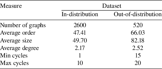
We do not enforce the odd-size constraint, as doing so would overly restrict the diversity of instances and limit the applicability of the dataset. Basic statistics of the resulting dataset are summarized in Table 1.
3.1.1 In-distribution dataset
The in-distribution dataset consists of 1300 exceptional graphs and 1300 decomposable graphs, for a total of 2600 instances.
A tadpole
$T_{m,n}$
 is the graph obtained by concatenating a cycle with
$m$
 vertices,
$C_m$
 , and a path with
$n+1$
 vertices,
$P_{n+1}$
 , with an edge from any vertex of
$C_m$
 to a pendant (vertex of degree one) of
$P_n$
 for
$m \geq 3$
 and
$n\geq 1$
 . Let
$\mathcal {P}$
 and
$\mathcal {T}$
 denote the full sets of path and tadpole graphs, respectively. Also, let
$\mathcal {P}_{\mathrm {even}}$
 denote the set of even-length paths (even size), and
$\mathcal {T}_{3, \mathrm { odd}}$
 the set of tadpole graphs with
$m = 3$
 and odd
$n$
 .
Among the exceptional graphs, 300 instances consist of:
-
• 100 odd-length paths;
-
• 100 odd-length cycles;
-
• 100 tadpole graphs with $m = 3$
and even
$n$
.


The remaining 1000 exceptional graphs are hand-crafted following the inductive construction of the class
$\mathfrak {T}$
 in Theorem 1 (excluding tadpole graphs). Specifically, each graph is constructed by identifying a degree-two vertex belonging to a triangle in a base graph from
$\mathfrak {T}$
 with a pendent vertex of degree one in a graph drawn from
$\mathcal {P}_{\mathrm {even}} \cup \mathcal {T}_{3, \mathrm {odd}}$
 .
Statistics for in-distribution and OOD datasets.

Table 1 Long description
The table consists of three columns: Measure, In-distribution dataset, and Out-of-distribution dataset.
* Number of graphs: 2600 for in-distribution and 520 for out-of-distribution.
* Average order: 47.41 for in-distribution and 66.03 for out-of-distribution.
* Average size: 49.70 for in-distribution and 82.18 for out-of-distribution.
* Average degree: 2.17 for in-distribution and 2.52 for out-of-distribution.
* Min cycles: 1 for in-distribution and 15 for out-of-distribution.
* Max cycles: 10 for in-distribution and 20 for out-of-distribution.
The decomposable subset is constructed analogously. It includes:
-
• 100 even-length paths;
-
• 100 even-length cycles;
-
• 100 tadpole graphs with $m = 3$
and odd
$n$
,


with the remaining 1000 instances generated via a similar inductive procedure. To ensure decomposability, pendant vertices from at least one graph in
$\mathcal {P} \setminus \mathcal {P}_{\mathrm {even}}$
 or
${\mathcal {T} \setminus \mathcal {T}_{3, \mathrm {odd}}}$
 are identified with a vertex of degree two in the base graph. This ensures that the resulting graph is still a cactus graph with maximum degree of three, but no longer satisfies the exceptional structural constraints of
$\mathfrak {T}$
 and is thus decomposable.
In addition, we include some adversarial decomposable instances obtained by deleting one or more edges from exceptional graphs while maintaining connectivity and decomposability. All graphs in the in-distribution dataset contain at least one cycle and at most ten cycles.
3.1.2 OOD dataset
The OOD dataset consists of 260 exceptional and 260 decomposable graphs instances for a total of 520 instances. These instances follow the same structural constraints as the in-distribution data, but are deliberately constructed to differ in scale and complexity.
Exceptional OOD graphs are generated using the same rules as their in-distribution counterparts, but are larger on average in both order and size, containing at least 15 and at most 20 cycles. Each decomposable OOD graph is obtained by modifying its exceptional counterpart through the addition or removal of one to three edges, ensuring that the graph becomes decomposable while remaining structurally similar. This design creates pairs of graphs that differ minimally in structure, but belong to different classes, which tests the model’s ability to generalize beyond the training distribution.
3.2 Experimental setup
To ensure a controlled and reproducible comparison of GNN architectures, we design our experiments to isolate the impact of aggregation and update mechanisms, while minimizing variance from data splits and optimization effects.
3.2.1 Evaluation procedure
All experiments are conducted on the in-distribution dataset using an 80:20 train-validation split. Since random splits can significantly influence reported performance [Reference Qiu57, Reference Raste, Singh, Vaughan and Nair58], we adopt five-fold cross validation and report results averaged across folds. Importantly, the same splits are used across all models in each fold to ensure a fair and consistent baseline comparison.
OOD generalization is evaluated using the separate dataset described in Section 3.1. Models are trained exclusively on the in-distribution data, and performance on OOD instances is assessed without further fine-tuning. For embedding-space analysis and OOD evaluation, model checkpoints are selected based on the epoch achieving the highest validation accuracy within each fold. All reported metrics are averaged across folds to reduce variance.
3.2.2 Shared model architecture
To isolate architectural effects, we adopt a shared backbone architecture across all GNN variants. The only components that differ between models are the message aggregation and update functions specific to each architecture. Each input graph
$G_i = (V_i, E_i)$
 is defined by its node set
$V_i$
 and edge set
$E_i$
 , node features
$\{\mathbf {x}_v \mid v \in V_i\}$
 and a one-hot encoded class label
$\mathbf {y}_i \in \{0,1\}^2$
 .
Node features are passed through
$L = 3$
 message-passing layers to produce embeddings
$\mathbf {h}_v^{(L)}$
 . A relatively low number of layers is chosen to avoid over-smoothing, which was shown to be prevalent in GNNs [Reference Wu, Chen, Wang and Jadbabaie72]. Hidden layers use a dimensionality of 64 and the final node embeddings are projected to 16 dimensions. This choice reflects common practice in the GNN literature, where hidden dimensions typically range from 16 to 256 [Reference Hamilton, Ying and Leskovec27, Reference Hu, Fey, Zitnik, Dong, Ren, Liu, Catasta and Leskovec30, Reference Kipf and Welling38]. The message-passing process is as follows:

with initial embeddings
$\mathbf {h}_v^{(0)} = \mathbf {x}_v$
 . A LeakyReLU [Reference Maas, Hannun and Ng50] nonlinearity is applied after the first two layers:

where
$\mathrm {LeakyReLU}(z) = \max (\alpha z, z)$
 ,
$\alpha = 0.2$
 . We also apply graph-wide normalization with GraphNorm as proposed by Cai et al. [Reference Cai, Luo, Xu, He, Liu and Wang14]. The normalization is defined as

where
$\alpha , \beta $
 and
$\gamma $
 are learnable parameters, and
$\epsilon $
 is a small constant to prevent division by 0. Normalization is applied after each GNN layer prior to the nonlinearity (when applicable). This is done such that the node embeddings have an appropriate (learnable) distribution that is conducive to learning. GraphNorm has been shown to improve training stability, accelerate convergence and help with generalization in graph learning tasks [Reference Cai, Luo, Xu, He, Liu and Wang14].
3.3 Graph-level representation
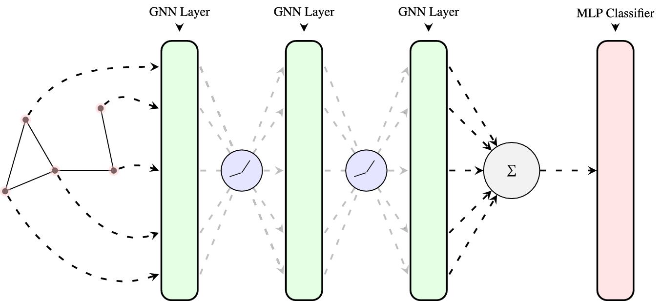
After the final message-passing layer, node embeddings are aggregated using global sum pooling to form a graph-level representation

The resulting graph embedding is passed through a multilayer perceptron (MLP) with a single hidden layer and a softmax output, producing predicted class probabilities
$\boldsymbol {\hat {y}}^{(i)} \in [0, 1]^2$
 . Models are trained using the binary cross-entropy loss:

and optimized using the Adam optimizer [Reference Kingma37]. An overview of the shared architecture is shown in Figure 3.
Illustration of the forward pass shared by the GNN models.

3.4 Aggregation
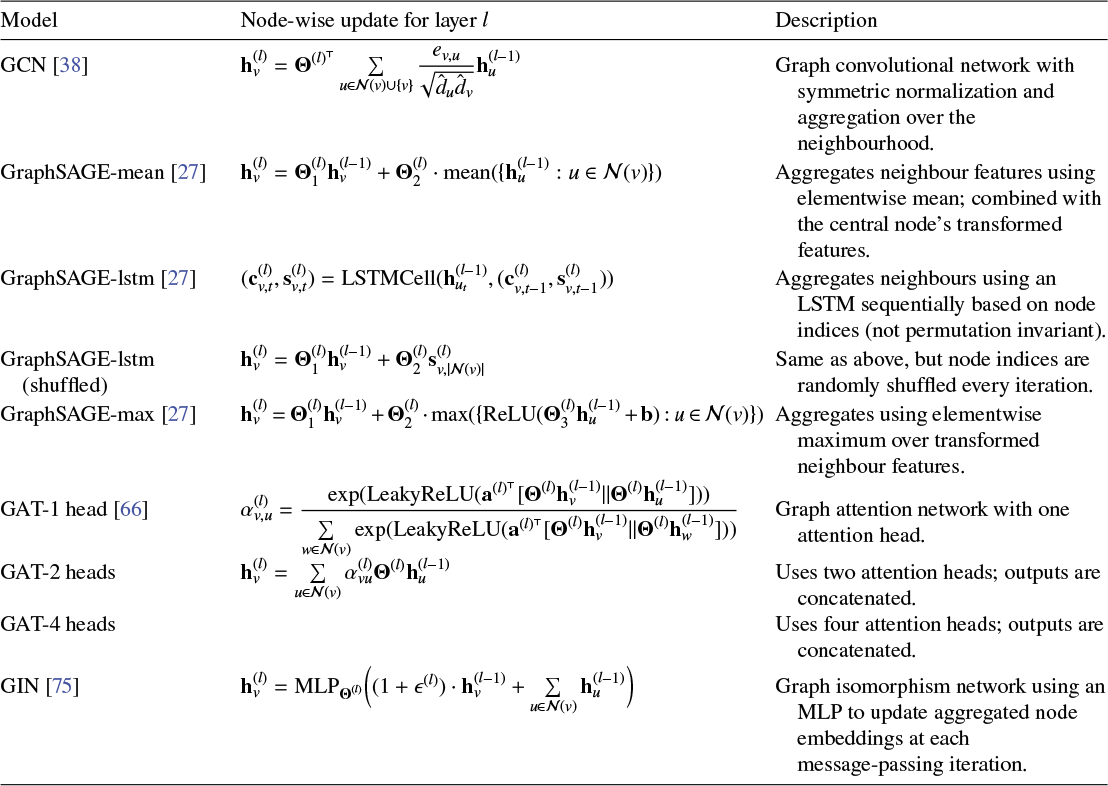
In this section, we present the aggregation schemes considered in this study. While not exhaustive, the selected architectures GCN [Reference Kipf and Welling38], GraphSAGE [Reference Hamilton, Ying and Leskovec27], GAT [Reference Veličkovi’c, Cucurull, Casanova, Romero, Lio and Bengio66] and GIN [Reference Xu, Hu, Leskovec and Jegelka75] represent some of the most widely adopted message passing neural network (MPNN) frameworks in recent years, due to their effectiveness across a range of graph learning tasks [Reference Hajibabaee, Malekzadeh, Heidari, Zad, Uzuner and Jones26, Reference Liang, Qian, Yu, Griffith and Golmie45, Reference Liu, Ong and Chen47, Reference Liu and Wang48, Reference Vrahatis, Lazaros and Kotsiantis67, Reference Zhang, Tong, Xu and Maciejewski77, Reference Zhang, Zhang and Wu78]. Table 2 summarizes the node-wise update formulation for each layer for some GNN models. These aggregation layers are implemented using PytorchGeometric (PyG) [Reference Fey and Lenssen18, Reference Fey19].
Summary of models considered in this study and their node-wise update formulations for each layer.

Table 2 Long description
The table consists of three columns: Model, Node-wise update for layer l, and Description.
* G C N: h sub v super (l) = Theta super (l) transpose summation over u in N(v) union {v} of (e sub v,u / sqrt(d-hat sub u d-hat sub v)) h sub u super (l-1). Described as a graph convolutional network with symmetric normalization.
* GraphSAGE-mean: h sub v super (l) = Theta sub 1 super (l) h sub v super (l-1) + Theta sub 2 super (l) dot mean({h sub u super (l-1) : u in N(v)}). Aggregates neighbor features using elementwise mean.
* GraphSAGE-lstm: (c sub v,t super (l), s sub v,t super (l)) = L S T M Cell(h sub u sub t super (l-1), (c sub v,t-1 super (l), s sub v,t-1 super (l))). Aggregates neighbors sequentially using an L S T M.
* GraphSAGE-lstm (shuffled): h sub v super (l) = Theta sub 1 super (l) h sub v super (l-1) + Theta sub 2 super (l) s sub v, |N(v)| super (l). Same as above but with random shuffling.
* GraphSAGE-max: h sub v super (l) = Theta sub 1 super (l) h sub v super (l-1) + Theta sub 2 super (l) dot max({ReLU(Theta sub 3 super (l) h sub u super (l-1) + b) : u in N(v)}). Aggregates using elementwise maximum.
* G A T-1 head: alpha sub v,u super (l) = exp(LeakyReLU(a super (l) transpose [Theta super (l) h sub v super (l-1) || Theta super (l) h sub u super (l-1)])) all over summation over w in N(v) of the same exp term. A graph attention network with one head.
* G A T-2 heads: h sub v super (l) = summation over u in N(v) of alpha sub vu super (l) Theta super (l) h sub u super (l-1). Uses two concatenated attention heads.
* G A T-4 heads: Formulation omitted. Uses four concatenated attention heads.
* G I N: h sub v super (l) = M L P sub Theta super (l) ((1 + epsilon super (l)) dot h sub v super (l-1) + summation over u in N(v) of h sub u super (l-1)). A graph isomorphism network using an M L P for updates.
3.4.1 Complexity
Determining if two graphs are isomorphic is NP-intermediate, with the best known general-purpose algorithm running in quasi-polynomial time [Reference Babai5]. For a graph with
$N$
 nodes and feature dimensionality
$F$
 , the forward pass for inference can be implemented in polynomial time and space. In the worst-case setting of dense graphs, models such as GCN, GAT, GraphSAGE (mean and max) exhibit
$O(N^2F + NF^2)$
 time complexity and
$O(N^2 + F^2 + NF)$
 space complexity [Reference Blakely, Lanchantin and Qi9]. Multi-head attention in GAT introduces a multiplicative factor proportional to the number of heads. We note that GIN and GraphSAGE-lstm will incur additional per layer costs for MLP and LSTM, respectively.
4 Experimental results and discussion
In this section, we will present and discuss the results obtained from 500 epochs of training for each model. We present training curves, confusion matrices, as well as principal component analysis (PCA) [Reference Abdi and Williams1] and t-distributed stochastic neighbour embedding (t-SNE) [Reference van der Maaten and Hinton65] visualizations of the embeddings. PCA enables us to analyse the intrinsic dimensionality of the embeddings generated, while t-SNE allows us to create a map in a lower-dimensional space where neighbouring points (similar data points) in the original high-dimensional space remain close together. We show that in certain cases, the models are able to generalize to some extent with the right initial node embeddings and aggregation schemes.
Training was conducted on an NVIDIA RTX A5000 GPU over a span of three days. A detailed summary of the hyper-parameters used in this study is provided in Table A1 in Appendix A. A separate training sequence of 2500 epochs was also further conducted on the two best models based on validation accuracy, which happen to be GraphSAGE-lstm [Reference Hamilton, Ying and Leskovec27] and GIN [Reference Xu, Hu, Leskovec and Jegelka75]. In this section, we present the results on learning dynamics of each GNN, and the best validation and OOD accuracies obtained by each.
4.1 Learning dynamics
Figures 4 and 5 illustrate the learning dynamics of the corresponding GNN architectures over 500 training epochs under two initialization regimes, which are constant node features and one-hot-degree as initial node features. By holding the training protocol fixed while varying only the initial node information, these experiments isolate how architectural inductive bias interacts with minimal node-level signals to enable stable learning and generalization. Training times are comparable across architectures (approximately 350 seconds on average), with the exception of the shuffled GraphSAGE-lstm variant (approximately 900 seconds), where the additional cost arises from per-iteration node-index shuffling.
Accuracy learning curves (mean
$\pm $
 std across five folds) for training, validation and OOD splits using constant node features.

Accuracy learning curves (mean
$\pm $
 std across five folds) for training, validation and OOD splits using one-hot-degree node features.

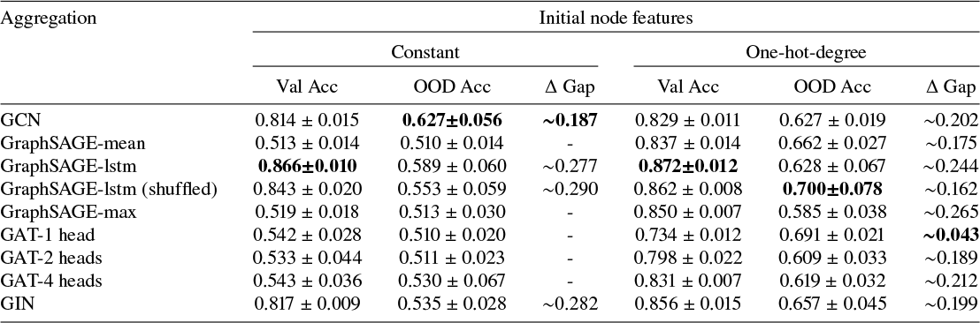
Under constant initialization (Figure 4), most architectures achieve high training accuracy but fail to generalize, collapsing to near-random performance on both validation and OOD splits. This behaviour indicates that message passing alone is frequently insufficient to recover the structural signal required by the task of distinguishing decomposable and exceptional graphs. Only GCN, GIN and the lstm-based GraphSAGE variants achieve nontrivial validation accuracy, stabilizing above 80% on average across five folds. These models share stronger aggregation or update mechanisms either near injective aggregation [Reference Xu, Hu, Leskovec and Jegelka75] or sequential neighbourhood integration, suggesting that increased architectural expressivity partially compensates for the absence of explicit node features. Nevertheless, even these architectures exhibit pronounced degradation on OOD graphs, revealing a limitation in extrapolating learned representations to graphs with substantially larger size or higher-order structure.
Introducing one-hot-degree as initial node features (Figure 5) fundamentally alters the learning behaviour. Architectures that previously failed to generalize, such as SAGE-mean, SAGE-max and all GAT variants, now converge reliably, exhibit reduced variance across folds, and achieve consistently higher validation and OOD accuracy. Across models, training and validation accuracy typically stabilize within the first 100 epochs, while OOD performance continues to improve thereafter, indicating that even with minimal local structural information, it is possible to achieve stable representation learning and extrapolation. These results suggest that degree features can help break representational symmetry and allow message passing to exploit local structural cues more effectively.
We further quantify these effects in Table 3 and analyse the corresponding embedding spaces in Section 4.3 to explain the observed differences in generalization behaviour.
Average validation and OOD accuracy of various aggregation schemes (
$\pm $
 std) and corresponding differences between validation and OOD accuracy (
$\Delta $
 Gap) for 500 epochs.

Table 3 Long description
The table is structured with a primary header row for Initial node features, split into Constant and One-hot-degree. Each category contains three sub-columns: Val Acc, O O D Acc, and Delta Gap.
* G C N: Constant features show Val Acc 0.814 plus or minus 0.015, O O D Acc 0.627 plus or minus 0.056, and Delta Gap tilde 0.187. One-hot-degree features show Val Acc 0.829 plus or minus 0.011, O O D Acc 0.627 plus or minus 0.019, and Delta Gap tilde 0.202.
* Graph S A G E-mean: Constant features show Val Acc 0.513 and O O D Acc 0.510. One-hot-degree features show Val Acc 0.837 and O O D Acc 0.662.
* Graph S A G E-l s t m: Constant features show Val Acc 0.866 plus or minus 0.010 and O O D Acc 0.589. One-hot-degree features show Val Acc 0.872 plus or minus 0.012 and O O D Acc 0.628.
* Graph S A G E-l s t m (shuffled): Constant features show Val Acc 0.843 and O O D Acc 0.553. One-hot-degree features show Val Acc 0.862 and O O D Acc 0.700 plus or minus 0.078.
* Graph S A G E-max: Constant features show Val Acc 0.519 and O O D Acc 0.513. One-hot-degree features show Val Acc 0.850 and O O D Acc 0.585.
* G A T-1 head: Constant features show Val Acc 0.542 and O O D Acc 0.510. One-hot-degree features show Val Acc 0.734 and O O D Acc 0.691 with a Delta Gap of tilde 0.043.
* G A T-2 heads: Constant features show Val Acc 0.533 and O O D Acc 0.511. One-hot-degree features show Val Acc 0.798 and O O D Acc 0.609.
* G A T-4 heads: Constant features show Val Acc 0.543 and O O D Acc 0.530. One-hot-degree features show Val Acc 0.831 and O O D Acc 0.619.
* G I N: Constant features show Val Acc 0.817 and O O D Acc 0.535. One-hot-degree features show Val Acc 0.856 and O O D Acc 0.657.
4.2 Comparative performance and OOD generalization
Table 3 reports the best average validation and OOD accuracies across five folds for each architecture after 500 training epochs. We observe several trends, which are as follows.
-
• Incorporating one-hot-degree features improves validation accuracy and substantially reduces performance variance across folds for nearly all architectures. In addition, the gap between in-distribution and OOD accuracy is reduced, indicating improved robustness under distribution shift.
-
• The GraphSAGE-lstm variants achieve the highest validation accuracy overall, followed closely by GIN. Notably, the unshuffled GraphSAGE-lstm outperforms its shuffled counterpart on validation data, but this comes at the cost of reduced OOD performance. Because the dataset is constructed with an arbitrary but fixed node ordering, this behaviour suggests that the unshuffled model may exploit order-dependent patterns that do not generalize. Shuffling node indices act as a regularizer, reducing validation accuracy while improving OOD robustness.
-
• GAT architectures exhibit lower validation accuracy than the top-performing models even with degree features, but their OOD performance is comparatively strong, where it is surpassed only by the shuffled GraphSAGE-lstm. We observe that increasing the number of attention heads in GAT consistently improves training and validation accuracy, but worsens OOD performance. This is highly suggestive that higher-capacity attention mechanisms more readily overfit to an in-distribution structure.
-
• GIN performs strongly on training and validation data, consistent with its known theoretical expressivity equivalent to the Weisfeiler–Lehman test [Reference Xu, Hu, Leskovec and Jegelka75]. With the task of classifying decomposable and exceptional graphs being equivalent to determining isomorphism to a graph in $\mathfrak {T}'$
, it is no surprise that GINs performed well in this setting. However, as with most architectures considered, GIN performance degrades on OOD graphs, suggesting that expressive aggregation alone may overfit and does not guarantee robustness to changes in graph size or structural complexity.

Taken together, these results demonstrate that while expressive aggregation can partially compensate for limited node features, its effectiveness is highly architecture dependent and fragile under distribution shift. For the task of classifying decomposable and exceptional graphs, only a small subset of architectures sustains meaningful generalization without explicit node information. With appropriate aggregation mechanisms and minimal structural node features, we show that GNNs can achieve high in-distribution accuracy and limited but nontrivial generalization to unseen graph distributions.
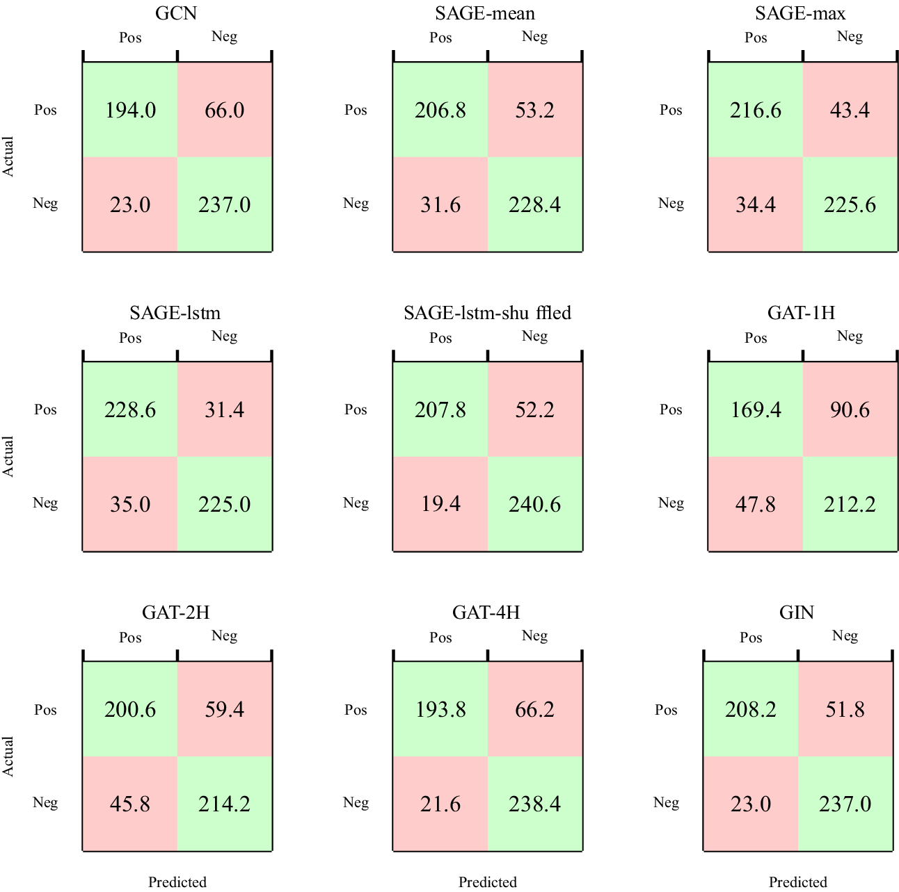
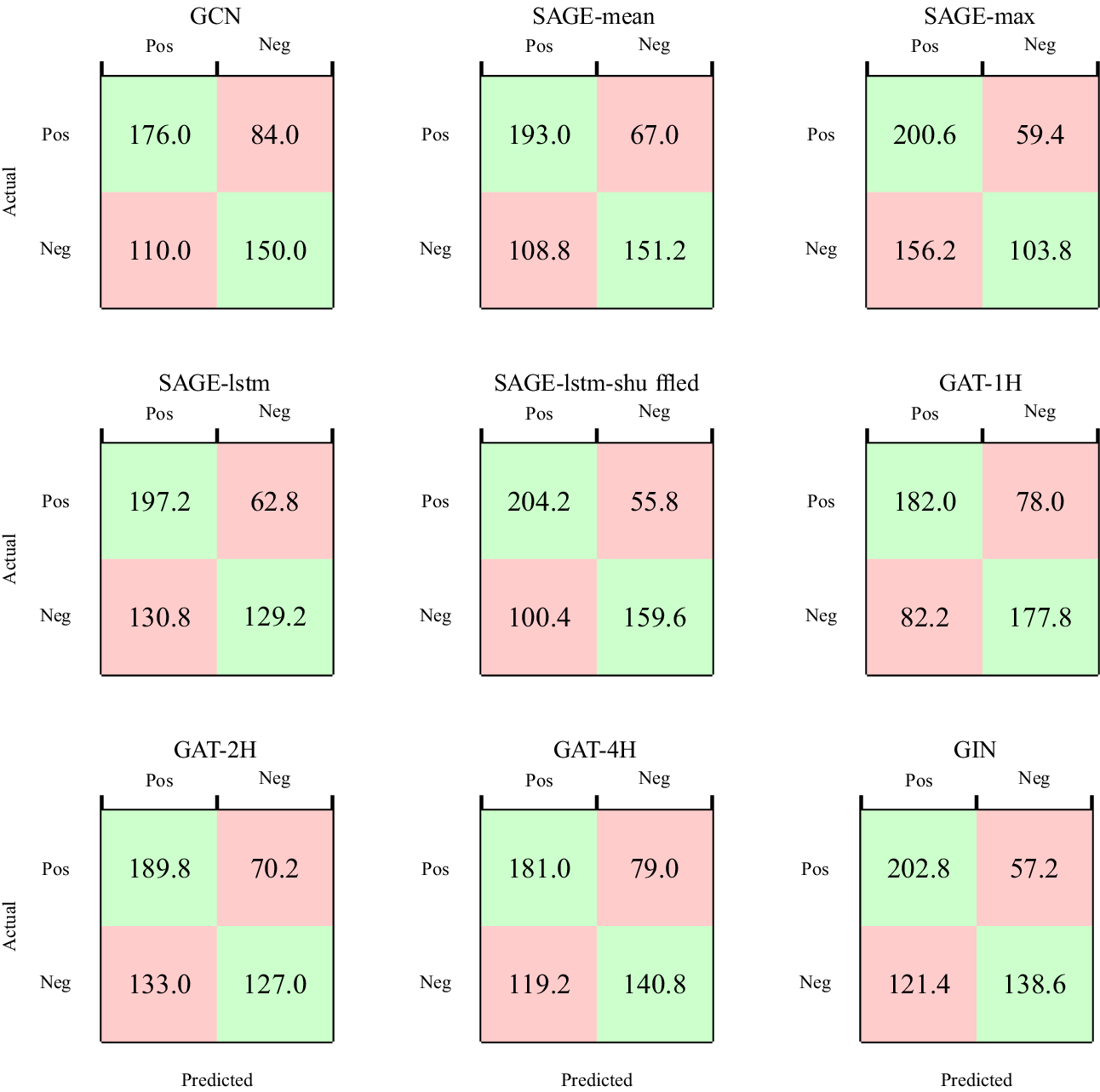
Detailed confusion matrices for the validation and OOD splits are reported in Figures A1 and A2, respectively, in Appendix A. On the validation set, predictions are generally well balanced across all architectures, with no strong bias towards either class. In contrast, evaluation on the OOD split reveals a consistent shift across most models towards increased false positives such that exceptional graphs are increasingly misclassified as decomposable.
Inspection of the graph distributions suggests that this behaviour is driven by a distributional bias. In the in-distribution training set, decomposable graphs tend to have larger order and size on average than exceptional graphs. As a result, models appear to rely on coarse graph-scale statistics, leading to an over-prediction of the decomposable class when confronted with larger or structurally more complex OOD graphs. Notably, the single-head GAT is the only architecture that does not exhibit this bias to the same extent, maintaining a more balanced error profile under distribution shift. This observation further supports the conclusion that single-head attention in GAT encourages the learning of more generalizable structural cues rather than over-reliance on size-related artefacts, despite their lower performance on the training and validation set.
4.3 Embedding analysis
It has been shown that the performance of many message passing GNNs degrades in the absence of node features [Reference Cai and Wang13, Reference Errica, Podda, Bacciu and Micheli17]; however, little work has been done to show why that is the case. In our results, we show that this is not the case in general and it is possible for some GNNs to learn meaningful representations related to graph structure despite the lack of initial node features.
We observe that both mean and max aggregation fail when all vertices share identical initial embeddings. Our experiments further reveal that GATs, despite having a more complex aggregation scheme exhibit the same limitations, as evidenced by their degraded performance under constant node features. This behaviour can be explained by examining the GAT aggregation rule, as shown as follows:

Suppose
$\mathbf {h}_v^{(l-1)} = \mathbf {h}_u^{(l-1)} = \mathbf {h}^{(l-1)}$
 for all
$v,u \in V(G)$
 , then

Following this,

This implies that under uniform initial embeddings, GAT layers reduce to a linear transformation applied identically to each node. This results in a complete loss of structural information. Due to the fact that each subsequent layer propagates identical representations, increasing network depth does not resolve the degeneracy. The same phenomenon also occurs in the improved GAT variant proposed in [Reference Brody, Alon and Yahav12], which relocates the attention vector outside the nonlinearity but does not address collapse under uniform features. Analogous derivations apply to GraphSAGE with mean and max aggregation as examples shown in [Reference Xu, Hu, Leskovec and Jegelka75]. As a consequence, when node features are identical or nearly identical, GATs and similar architectures struggle to distinguish graph structure.
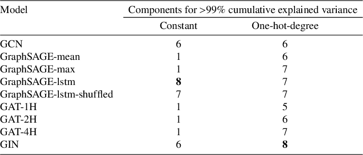
The empirical evidence in Table 4 demonstrates that including degree as a node feature allows GraphSAGE-mean, GraphSAGE-max and GAT to generate embeddings with substantially higher effective dimensionality after message passing. Conversely, using constant node features results in embeddings that are effectively linear. In contrast, aggregation schemes like GCN and GIN do not suffer from this to the same extent, as their aggregation schemes have partially recover structural information such as node degree (for example, the
$\sqrt {\hat {d}_u \cdot \hat {d}_v}$
 normalization term in GCN and the summation over neighbouring embeddings in GIN and GraphSAGE-lstm; see Table 2). Consequently, the performance of GCN, GIN and GraphSAGE-lstm with constant node features remains relatively close to the case where degree information is included explicitly, though explicit degree features still yield a modest improvement.
Number of principal components for
$>$
 99% cumulative explained variance for each model, trained on constant initialized node embeddings and one-hot-degree initialized node embeddings.

Table 4 Long description
The table consists of three columns: Model, Constant initialization, and One-hot-degree initialization.
* G C N: 6 for Constant, 6 for One-hot-degree.
* Graph S A G E-mean: 1 for Constant, 6 for One-hot-degree.
* Graph S A G E-max: 1 for Constant, 7 for One-hot-degree.
* Graph S A G E-l s t m: 8 for Constant, 7 for One-hot-degree.
* Graph S A G E-l s t m-shuffled: 7 for Constant, 7 for One-hot-degree.
* G A T-1 H: 1 for Constant, 5 for One-hot-degree.
* G A T-2 H: 1 for Constant, 6 for One-hot-degree.
* G A T-4 H: 1 for Constant, 7 for One-hot-degree.
* G I N: 6 for Constant, 8 for One-hot-degree.
The highest value for Constant initialization is 8 (Graph S A G E-l s t m) and the highest for One-hot-degree is 8 (G I N).
4.3.1 Principal component analysis
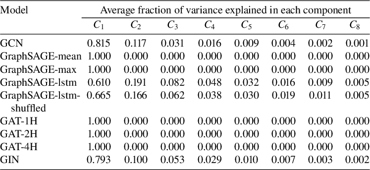
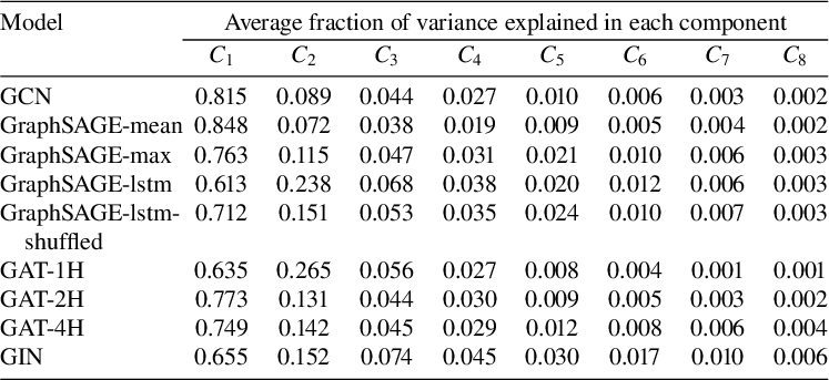
To quantify the intrinsic dimensionality of the embeddings generated, we use PCA [Reference Abdi and Williams1] to measure the percentage of explained variance in each principal component. For full PCA plots of the validation set for both the models trained on the dataset with constant node features and one-hot-degree initialized node features, we refer readers to Tables A2 and A3, respectively, in Appendix A.
Table 4 along with Tables A2 and A3 in Appendix A analyse the intrinsic dimensionality of the learned graph embeddings under constant and one-hot-degree node initializations. When initialized with constant node features, the majority of message-passing architectures fail to learn meaningful structural representations. This observation can be seen as the final graph embeddings collapse onto a one-dimensional subspace, with a single principal component accounting for almost all of the cumulative variance. This collapse indicates a severe loss of representational diversity and explains the observed failure to generalize beyond the training set. In contrast, only GCN, GIN and the lstm-based GraphSAGE variants exhibit higher intrinsic dimensionality, suggesting that these architectures are capable of partially recovering structural information through aggregation alone.
Introducing one-hot-degree features substantially changes this behaviour (see Table A3). Most architectures now produce embeddings with significantly higher intrinsic dimensionality, indicating that degree information provides a stable reference that allows message passing to construct richer structural representations. Notably, GATs achieve strong generalization despite maintaining comparatively low intrinsic dimensionality (approximately five principal components explaining
$>$
 99% of the variance). This suggests that compact but structured representations may be preferable for robustness under distribution shift. Conversely, architectures such as GIN and GraphSAGE-lstm that generate higher-dimensional embeddings often achieve stronger in-distribution performance, but exhibit degraded OOD accuracy, consistent with overfitting to distribution-specific structural patterns.
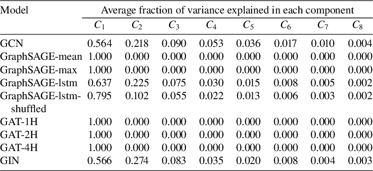
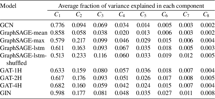
Tables A4 and A5 in Appendix A show the PCA-explained variance profiles of embeddings produced by the trained models on the OOD set, for datasets with constant node features and one-hot-degree initializations, respectively. In general, the embeddings exhibit intrinsic dimensionality trends that closely mirror those observed on the in-distribution data. For the OOD set, achieving over 99% explained variance requires a larger number of principal components and the tail components account for a higher fraction of variance on average. This indicates a broader dispersion of embedding representations in the OOD distribution. We propose that this effect arises from the increased average size and order of graphs in the OOD set, which introduces greater structural variability. Consequently, these results suggest that the observed degradation in predictive performance is unlikely to stem from insufficiently expressive embeddings. Instead, it points to a mismatch between the learned decision boundary and the expanded graph distribution encountered at test time, particularly for larger graphs outside the training distribution.
4.3.2 Misclassified graphs
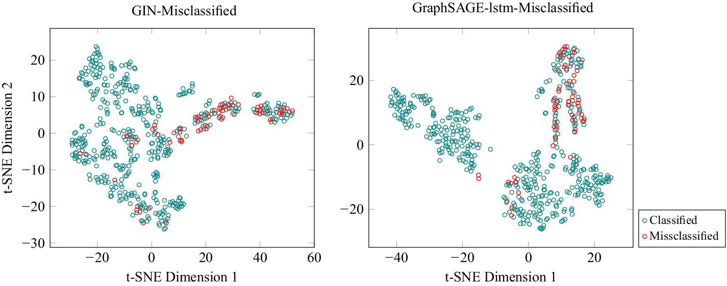
By extracting the learned graph embeddings and inspecting the misclassified instances, we observe that most in-distribution misclassifications cluster within localized regions of the embedding space rather than being uniformly dispersed (see Figure 6). These regions are dominated by simple graphs such as path, cycle and tadpole graphs, indicating that these structures induce systematic ambiguity for the models. Further inspection of the predicted class probabilities reveals that, for these graph families, the models typically assign near-uniform probabilities (approximately 50–50) across classes. This suggests that the learned representations capture insufficient discriminative signals for these motifs, rather than exhibiting a strong but incorrect bias towards a particular class. In other words, the models appear uncertain rather than confidently wrong, pointing to an inherent representational limitation when distinguishing these structurally simple yet ambiguous graphs.
Missclassified graphs for GIN and GraphSAGE-lstm for the validation set (fold two). The cluster of missclassified graphs (in red) consists of paths, cycles and tadpole graphs. Similar clusters exist for the embeddings generated by other aggregation schemes.

Excluding these simple graphs, the remaining misclassified graphs do not exhibit a consistent structural pattern and are scattered uniformly throughout the dataset. In these cases, however, the top-performing models tend to be confidently incorrect, often assigning high probability to the wrong class. Notably, despite these errors, the overall prediction distribution on the validation set remains balanced, with no systematic preference for either class. This indicates that misclassifications are not driven by class imbalance or global bias.
The OOD set does not contain path, cycle or tadpole graphs. Nevertheless, we expect similar outcomes as in the in-distribution set to persist for these graphs. For OOD graphs, we observe that models frequently misclassify graphs with high confidence, predominantly prediction on the decomposable class. We attribute this behaviour to a distributional shift in graph size and order, where decomposable graphs in the training sets tend to have higher average size, causing the models to rely on size-correlated features that do not generalize to the OOD dataset. While this effect is present across architectures, it is less pronounced in GAT-based models than other well-performing models in the validation such as GIN and GraphSAGE-lstm variants. We suspect that it is due to the lower intrinsic dimensionality of the embeddings generated. This allows the embeddings to be more generalizable to unseen distributions instead of overfitting.
Figure 7 visualizes OOD embeddings using t-SNE [Reference van der Maaten and Hinton65] for both GAT and GIN. The embeddings produced by GAT-1H exhibit less polarized decision regions, resulting in less one-sided predictions. However, increasing the number of attention heads increases the tendency to predict decomposable graphs, suggesting that additional heads may encourage overfitting to in-distribution structural statistics rather than improving robustness to distributional shift. This behaviour aligns with our PCA analysis, which shows that embeddings produced by GIN and GraphSAGE-lstm exhibit substantially higher intrinsic dimensionality. This implies that increased model capacity that captures in-distribution variability is at the expense of generalization to OOD graph structures.
Comparison of true and predicted labels for GAT-1H and GIN, with normalization and one-hot encoded degree as initial features for the OOD set (fold two). We observe that for aggregation schemes other than GAT-1H, the predictions tend to bias towards decomposable graphs heavily.

4.4 Long-term behaviour of the models
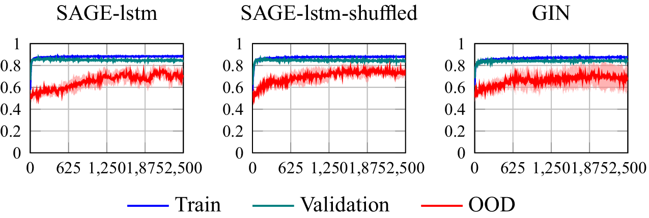
We ran extended training (2500 epochs) for the top-performing architectures on the validation set, which are GIN and the GraphSAGE-lstm variants. Figure 8 shows the training, validation and OOD accuracies over the full 2500 epochs (mean
$\pm $
 std across five folds).
Accuracy learning curves (mean
$\pm $
 std across five folds) for training, validation and OOD splits using constant node features.

First, training and validation accuracies stabilize near approximately 85% well before 2500 epochs, while OOD accuracy continues to improve after epoch 500. This divergence indicates that prolonged training can yield representations that generalize better to OOD instances even after the conventional train/validation signals appear to have converged. Second, the different architectures exhibit distinct reliability across folds, where the shuffled GraphSAGE-lstm variant produces the most stable OOD performance (small variance between folds), whereas GIN shows substantially greater variability, where some folds reach OOD performance comparable to training and validation, while others stop improving at approximately 60% accuracy.
We inspected the fold contents to identify obvious distributional causes (for example, different counts of paths, cycles or tadpole graphs across folds), but found no meaningful differences in these distributions. Thus, the observed GIN sensitivity appears not to be explained by a sampling imbalance. Possible contributors include stochastic optimization effects (initialization and SGD noise), model inductive bias and capacity, or differing reliance on size-correlated features that fail to generalize to the OOD set. Resolving these possibilities is left to future work.
Taken together, these results provide evidence that: (1) extended training can improve OOD generalization for some architectures; and (2) model choice and architecture-specific behaviour (here, the stability advantage of shuffled GraphSAGE-lstm versus the fold sensitivity of GIN) materially affect OOD robustness. We therefore recommend that experimental evaluations of OOD generalization report OOD metrics across extended training runs and across multiple folds and/or seeds rather than relying on the epoch at which training and validation appears to converge.
5 Limitations and future work
5.1 Computational budget
Owing to limited compute resources, the extended 2500-epoch experiments were performed on the two top validation models (GIN and GraphSAGE-lstm variants) rather than across all nine architectures. This choice was made deliberately to: (1) exercise the highest-capacity, best-performing architectures; and (2) evaluate whether extended training yields consistent OOD gains for the most promising models. We acknowledge this selection is not exhaustive. Future work should expand long-run experiments to additional architectures as compute allows.
5.2 Dataset scale and design
Our dataset (training and validation set of 2600 graphs and OOD set of 520 graphs) is primarily hand-crafted to ensure coverage of the structural motifs relevant to the locally irregular edge-colouring decision problem. This domain-specific construction trades scale for careful control over specific graph patterns and adversarial instances. This may limit how broadly the quantitative results generalize to naturally occurring graphs. We therefore present our empirical findings as targeted evidence about GNN behaviour on this problem family rather than as universal claims about all graph-classification tasks.
5.3 Limited hyper-parameter exploration
Network training was performed for five folds and we report mean
$\pm $
 std and we did not perform exhaustive hyper-parameter sweeps or change random seeds. The fold-to-fold variability observed for GIN suggests that additional seeds, systematic hyper-parameter searches and a larger number of folds would be valuable to fully characterize architecture-level sensitivity. We therefore treat the long-run experiments as evidence of promising behaviour, not definitive proof that extended training universally improves OOD generalization.
5.4 Scope of aggregation schemes
We focused on widely used aggregation schemes (GCN, GraphSAGE, GAT and GIN) as representative baselines, supported by their prevalence in the literature and in common frameworks. This is evidenced by the foundational papers for these models being among the most cited in graph learning [Reference Hamilton, Ying and Leskovec27, Reference Kipf and Welling38, Reference Veličkovi’c, Cucurull, Casanova, Romero, Lio and Bengio66, Reference Xu, Hu, Leskovec and Jegelka75]. Overall, surveys and benchmarks regularly list these models as prototypical GNN architectures [Reference Hu, Fey, Zitnik, Dong, Ren, Liu, Catasta and Leskovec30, Reference Morris, Kriege, Bause, Kersting, Mutzel and Neumann53]. However, other alternative aggregation and readout strategies exist and may be better tailored to the locally irregular edge-colouring problem. Future work should explore broader families of GNNs and non-GNN baselines (graph kernels, classical combinatorial methods) to better delineate where GNNs succeed and fail on this task.
6 Concluding remarks
In this work, we investigated the ability of modern GNNs to distinguish between decomposable and exceptional graphs, a decision problem rooted in locally irregular edge-colourings. Across a range of widely used architectures, we show that GNNs can reliably extract discriminative structural information even when provided with minimal node features, indicating that message-passing alone is sufficient to encode nontrivial graph properties relevant to this task. Among the evaluated models, GraphSAGE-lstm and GIN consistently achieved the strongest performance across in-distribution settings, highlighting the importance of architectural inductive bias for graph-level reasoning.
Beyond overall accuracy, our analysis reveals systematic failure modes that provide insight into current GNN limitations. While many architectures successfully separate graphs with richer or more irregular structure, simpler structures such as paths and cycles remain a source of ambiguity. These structures produce embeddings that are weakly separated and yield low-confidence predictions, suggesting that existing message-passing schemes struggle to distinguish certain structurally simple yet distinct graphs. Addressing these failure cases represents a clear direction for future work, either through enhanced aggregation schemes, structural features or hybrid approaches that integrate combinatorial reasoning.
We further demonstrate that embedding geometry and dimensionality play a critical role in generalization. We show that in constant settings, architectures like GraphSAGE-mean, GraphSAGE-max and even the more complex aggregation scheme GAT can fail to generate expressive embeddings due to inherent limitations in their message passing and update functions. Although higher-dimensional embeddings (as produced by GIN and GraphSAGE-lstm) are beneficial for in-distribution performance, lower-dimensional representations such as GAT with a single attention head can yield improved robustness under distributional shift. This trade-off highlights that expressivity alone is insufficient for OOD generalization and that architectural constraints may act as an implicit regularizer.
Importantly, we show that standard early-stopping criteria based on training or validation convergence may be insufficient in OOD settings. Despite early stabilization of training and validation accuracy, OOD performance continues to improve with prolonged training, suggesting that internal representations continue to evolve in ways that enhance robustness without affecting in-distribution metrics. This observation has practical implications for how GNNs are trained and evaluated when generalization beyond the training distribution is a priority.
Taken together, our results suggest that GNNs are not merely effective classifiers for this problem, but also valuable exploratory tools for discrete mathematics. By revealing both successes and systematic failure modes, GNNs can assist researchers in uncovering structural patterns, generating conjectures and guiding further theoretical or computational investigations. To facilitate continued progress and enabling the community to reproduce our results and extend the analysis to alternative architectures and graph families, our dataset and source code are available on GitHubFootnote 2 .
A Appendix
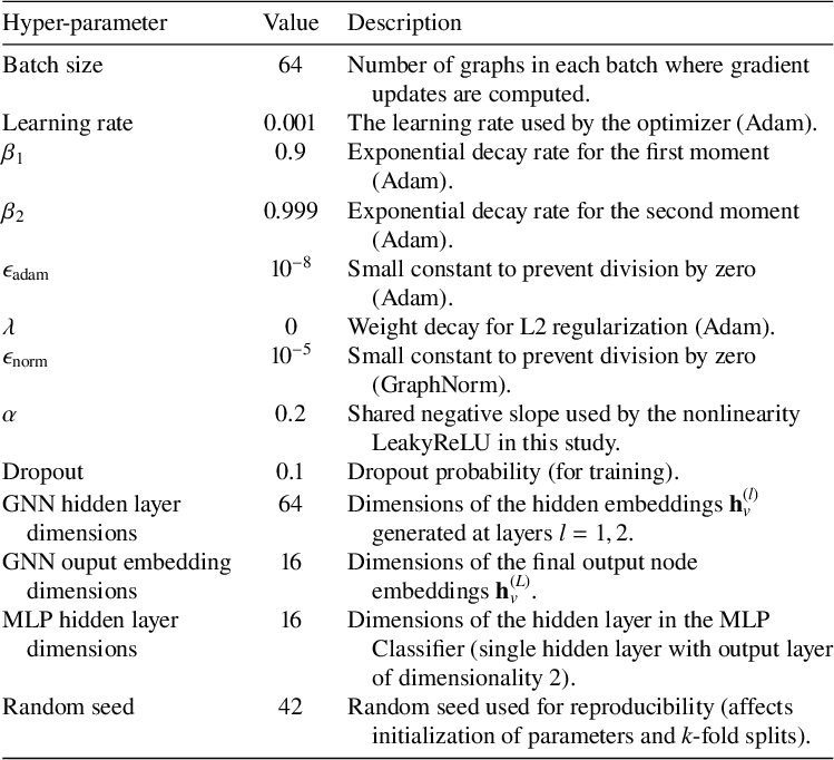
List of hyper-parameters and their values. Note that we did not perform systematic hyper-parameter tuning and sweeps due to computational cost. It is entirely possible to achieve better results by tuning the hyper-parameters.

Table A1 Long description
The table contains three columns: Hyper-parameter, Value, and Description.
* Batch size: 64. Number of graphs in each batch where gradient updates are computed.
* Learning rate: 0.001. The learning rate used by the optimizer Adam.
* beta sub 1: 0.9. Exponential decay rate for the first moment Adam.
* beta sub 2: 0.999. Exponential decay rate for the second moment Adam.
* epsilon sub adam: 10 super negative 8. Small constant to prevent division by zero Adam.
* lambda: 0. Weight decay for L 2 regularization Adam.
* epsilon sub norm: 10 super negative 5. Small constant to prevent division by zero GraphNorm.
* alpha: 0.2. Shared negative slope used by the nonlinearity LeakyReLU in this study.
* Dropout: 0.1. Dropout probability for training.
* G N N hidden layer dimensions: 64. Dimensions of the hidden embeddings h sub v super l generated at layers l equals 1, 2.
* G N N output embedding dimensions: 16. Dimensions of the final output node embeddings h sub v super L.
* M L P hidden layer dimensions: 16. Dimensions of the hidden layer in the M L P Classifier single hidden layer with output layer of dimensionality 2.
* Random seed: 42. Random seed used for reproducibility affects initialization of parameters and k-fold splits.
Confusion matrices of validation set with one-hot-encoded degree as node features of the best model over 500 epochs, detailing the TP, TN, FP, FN averaged over five folds. Positive instances are decomposable while negative instances are exceptional.

Confusion matrices of OOD set with one-hot-encoded degree as node features best model over 500 epochs, detailing the TP, TN, FP, FN averaged over five folds. Positive instances are decomposable while negative instances are exceptional.

Average explained PCA variance (eight components) over five folds for models trained on graphs with constant initialized node embeddings of the in-distribution validation set. Each column
$C_i$
 tabulates the average fraction of explained variance of each component
$i$
 .

Table A2 Long description
The table consists of nine rows representing different models and eight columns representing P C A components C sub 1 through C sub 8.
* G C N: C sub 1 = 0.815, C sub 2 = 0.117, C sub 3 = 0.031, C sub 4 = 0.016, C sub 5 = 0.009, C sub 6 = 0.004, C sub 7 = 0.002, C sub 8 = 0.001.
* GraphSAGE-mean: C sub 1 = 1.000, all other components are 0.000.
* GraphSAGE-max: C sub 1 = 1.000, all other components are 0.000.
* GraphSAGE-lstm: C sub 1 = 0.610, C sub 2 = 0.191, C sub 3 = 0.082, C sub 4 = 0.048, C sub 5 = 0.032, C sub 6 = 0.016, C sub 7 = 0.009, C sub 8 = 0.005.
* GraphSAGE-lstm-shuffled: C sub 1 = 0.665, C sub 2 = 0.166, C sub 3 = 0.062, C sub 4 = 0.038, C sub 5 = 0.030, C sub 6 = 0.019, C sub 7 = 0.011, C sub 8 = 0.005.
* G A T-1 H: C sub 1 = 1.000, all other components are 0.000.
* G A T-2 H: C sub 1 = 1.000, all other components are 0.000.
* G A T-4 H: C sub 1 = 1.000, all other components are 0.000.
* G I N: C sub 1 = 0.793, C sub 2 = 0.100, C sub 3 = 0.053, C sub 4 = 0.029, C sub 5 = 0.010, C sub 6 = 0.007, C sub 7 = 0.003, C sub 8 = 0.002.
Average explained PCA variance (eight components) over five folds for models trained on graphs with one-hot-degree initialized node embeddings of the in-distribution validation set. Each column
$C_i$
 tabulates the average fraction of explained variance of each component
$i$
 .

Table A3 Long description
The table consists of a header row and nine data rows. The columns are labeled Model, followed by C sub 1 through C sub 8, representing the eight P C A components.
* G C N: 0.815, 0.089, 0.044, 0.027, 0.010, 0.006, 0.003, 0.002.
* GraphSAGE-mean: 0.848, 0.072, 0.038, 0.019, 0.009, 0.005, 0.004, 0.002.
* GraphSAGE-max: 0.763, 0.115, 0.047, 0.031, 0.021, 0.010, 0.006, 0.003.
* GraphSAGE-l s t m: 0.613, 0.238, 0.068, 0.038, 0.020, 0.012, 0.006, 0.003.
* GraphSAGE-l s t m-shuffled: 0.712, 0.151, 0.053, 0.035, 0.024, 0.010, 0.007, 0.003.
* G A T-1 H: 0.635, 0.265, 0.056, 0.027, 0.008, 0.004, 0.001, 0.001.
* G A T-2 H: 0.773, 0.131, 0.044, 0.030, 0.009, 0.005, 0.003, 0.002.
* G A T-4 H: 0.749, 0.142, 0.045, 0.029, 0.012, 0.008, 0.006, 0.004.
* G I N: 0.655, 0.152, 0.074, 0.045, 0.030, 0.017, 0.010, 0.006.
Average explained PCA variance (eight components) over five folds for models trained on graphs with constant initialized node embeddings of the OOD set. Each column
$C_i$
 tabulates the average fraction of explained variance of each component
$i$
 .

Table A4 Long description
The table consists of nine rows representing different models and eight columns labeled C sub 1 through C sub 8 representing the principal components.
* G C N: C sub 1 = 0.564, C sub 2 = 0.218, C sub 3 = 0.090, C sub 4 = 0.053, C sub 5 = 0.036, C sub 6 = 0.017, C sub 7 = 0.010, C sub 8 = 0.004.
* GraphSAGE-mean: C sub 1 = 1.000, all other components are 0.000.
* GraphSAGE-max: C sub 1 = 1.000, all other components are 0.000.
* GraphSAGE-l s t m: C sub 1 = 0.637, C sub 2 = 0.225, C sub 3 = 0.075, C sub 4 = 0.030, C sub 5 = 0.015, C sub 6 = 0.008, C sub 7 = 0.005, C sub 8 = 0.002.
* GraphSAGE-l s t m-shuffled: C sub 1 = 0.795, C sub 2 = 0.102, C sub 3 = 0.055, C sub 4 = 0.022, C sub 5 = 0.013, C sub 6 = 0.006, C sub 7 = 0.003, C sub 8 = 0.002.
* G A T-1 H: C sub 1 = 1.000, all other components are 0.000.
* G A T-2 H: C sub 1 = 1.000, all other components are 0.000.
* G A T-4 H: C sub 1 = 1.000, all other components are 0.000.
* G I N: C sub 1 = 0.566, C sub 2 = 0.274, C sub 3 = 0.083, C sub 4 = 0.035, C sub 5 = 0.020, C sub 6 = 0.008, C sub 7 = 0.004, C sub 8 = 0.003.
Average explained PCA variance (eight components) over five folds for models trained on graphs with one-hot-degree initialized node embeddings of the OOD set. Each column
$C_i$
 tabulates the average fraction of explained variance of each component
$i$
 .

Table A5 Long description
The table consists of nine rows representing different models and eight columns labeled C 1 through C 8 representing the principal components.
* G C N: C 1 0.776, C 2 0.094, C 3 0.069, C 4 0.034, C 5 0.014, C 6 0.005, C 7 0.003, C 8 0.002.
* GraphSAGE-mean: C 1 0.858, C 2 0.058, C 3 0.038, C 4 0.020, C 5 0.013, C 6 0.006, C 7 0.003, C 8 0.002.
* GraphSAGE-max: C 1 0.579, C 2 0.217, C 3 0.099, C 4 0.046, C 5 0.029, C 6 0.015, C 7 0.006, C 8 0.004.
* GraphSAGE-lstm: C 1 0.611, C 2 0.163, C 3 0.093, C 4 0.067, C 5 0.035, C 6 0.018, C 7 0.005, C 8 0.003.
* GraphSAGE-lstm-shuffled: C 1 0.513, C 2 0.233, C 3 0.116, C 4 0.060, C 5 0.033, C 6 0.019, C 7 0.012, C 8 0.005.
* G A T-1 H: C 1 0.633, C 2 0.159, C 3 0.080, C 4 0.057, C 5 0.036, C 6 0.018, C 7 0.007, C 8 0.004.
* G A T-2 H: C 1 0.617, C 2 0.176, C 3 0.093, C 4 0.051, C 5 0.026, C 6 0.017, C 7 0.008, C 8 0.005.
* G A T-4 H: C 1 0.682, C 2 0.160, C 3 0.059, C 4 0.042, C 5 0.024, C 6 0.015, C 7 0.007, C 8 0.004.
* G I N: C 1 0.598, C 2 0.177, C 3 0.081, C 4 0.048, C 5 0.035, C 6 0.027, C 7 0.011, C 8 0.008.