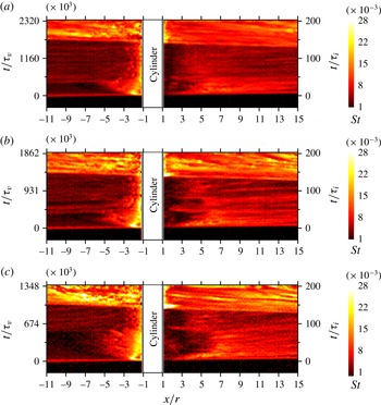
1 Introduction
In this study we examine the unsteady flow produced by a shock wave passing over a cylindrical obstacle fixed to a wall, for the case that the shock is of sufficient strength that the post-shock flow is supersonic. The interaction of a shock wave or blast wave with a wall-mounted obstacle can be viewed as a canonical problem that produces a variety of interesting non-stationary flow phenomena, but is also relevant in a number of physical situations. Shock waves propagating ahead of flame fronts and interacting with obstacles can produce localized hot spots in the flow field, leading to deflagration-to-detonation transition (Thomas et al. Reference Thomas, Ward, Williams and Bambrey2002; Gamezo, Ogawa & Oran Reference Gamezo, Ogawa and Oran2007). Predicting the response of a structure to an external explosion requires understanding the interaction between a blast wave and an obstacle (Ofengeim & Drikakis Reference Ofengeim and Drikakis1997). The interaction of compression waves with floor-mounted obstacles has also been suggested as a mechanism for reducing the strength of weak shock waves created by the passage of a high-speed train through a tunnel (Abe, Takayama & Itoh Reference Abe, Takayama and Itoh1997). In the present work, our primary focus is the interaction of the cylindrical obstacle with the post-shock supersonic flow rather than with the shock itself; in particular, we investigate how the development of the unsteady flow phenomena affects the instantaneous heat-transfer rates to the wall in the vicinity of the obstacle. This may be viewed as the unsteady counterpart of an oft-studied problem in high-speed aerodynamics, viz. the flow field produced by the interaction of a supersonic boundary-layer flow with a blunt obstacle. For the purposes of interpreting the results of the present study, a brief review of the important characteristics of this latter problem will be useful.
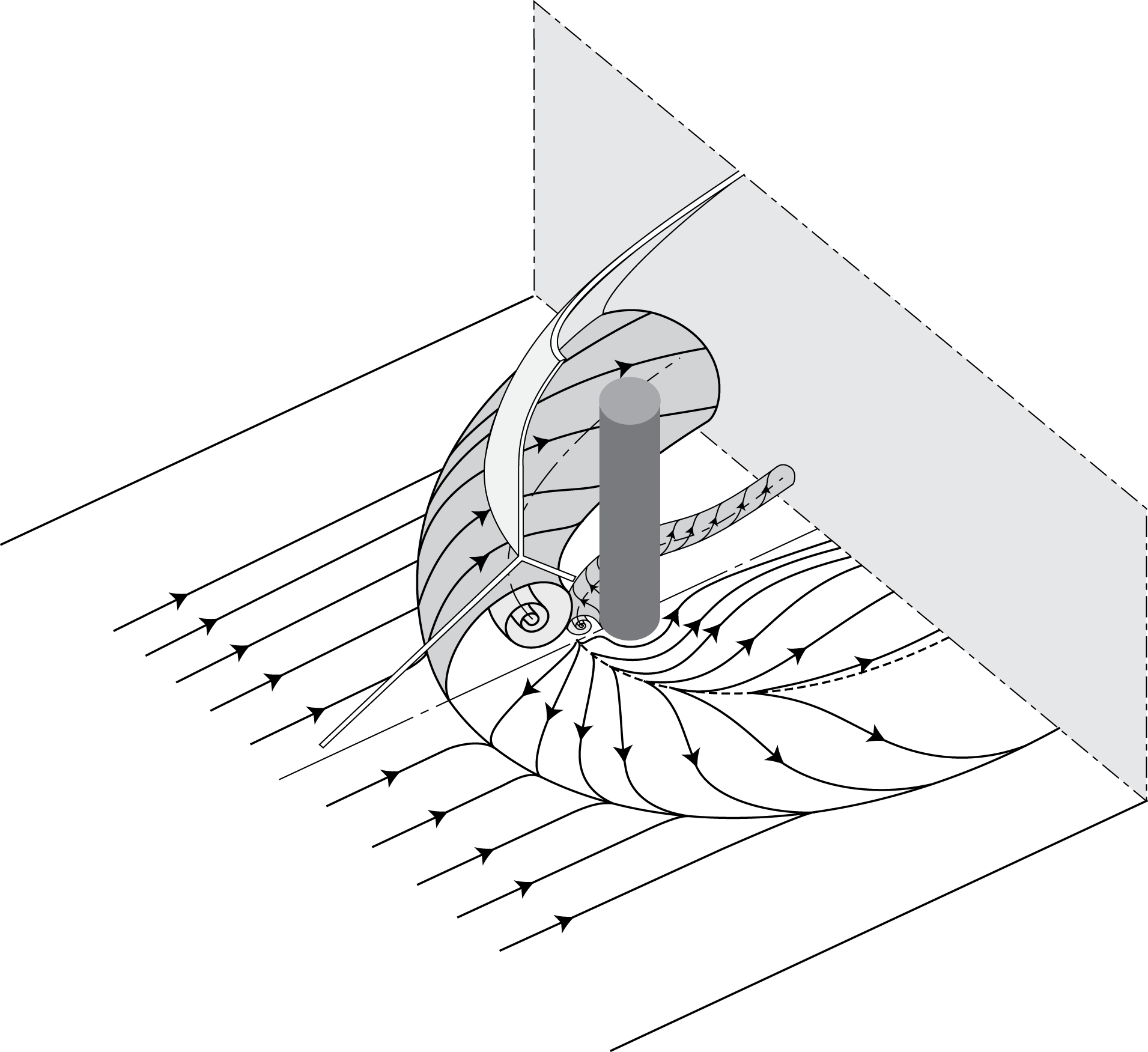
Major flow features generated in the supersonic boundary-layer flow over a wall-mounted cylinder. The solid and dashed arrowless lines on the wall indicate separation and attachment lines.

Even if we restrict the blunt obstacle to being a cylinder with axis oriented normal to the wall – or a hemicylindrical blunted fin, which produces the same upstream flow (Korkegi Reference Korkegi1971) – a large number of parameters are important to this problem: the undisturbed boundary-layer state (laminar, transitional, turbulent), the edge Mach number,
 $M$
, the ratio of cylinder radius to boundary-layer thickness,
 $r/\unicode[STIX]{x1D6FF}$
, the aspect ratio of the cylinder,
 $h/r$
, and a Reynolds number based on any one of these length scales,
 $Re$
. In the case that
 $h\gg \unicode[STIX]{x1D6FF}$
and the cylinder diameter is small in comparison to
 $\unicode[STIX]{x1D6FF}$
, the obstacle height becomes unimportant (Sedney & Kitchens Reference Sedney and Kitchens1977). In this limit, the primary upstream flow features are as depicted in figure 1 and can be summarized based on the work of a number of earlier authors (Korkegi Reference Korkegi1971; Sedney Reference Sedney1972; Sedney & Kitchens Reference Sedney and Kitchens1975, Reference Sedney and Kitchens1977; Dolling & Bogdonoff Reference Dolling and Bogdonoff1981; Hung & Clauss Reference Hung and Clauss1981; Özkan & Holt Reference Özkan and Holt1984; Dolling & Smiths Reference Dolling and Smiths1989; Özkan & Yüceil Reference Özkan and Yüceil1992; Lakshmanan & Tiwari Reference Lakshmanan and Tiwari1994; Tutty, Roberts & Schuricht Reference Tutty, Roberts and Schuricht2013) as follows. (i) In the plane of symmetry, the flow structures are similar to the two-dimensional shock-wave/boundary-layer interaction (SWBLI) produced, for example, by a forward-facing step, with a normal shock terminating at a lambda shock, and a separated region forming ahead of the shock. This is true whether the incoming boundary layer is laminar or turbulent. (ii) The upstream extent of the separated region measured from the leading edge of the cylinder (
 $S$
) is larger for a laminar boundary layer than for a turbulent one. (iii)
 $S$
depends on both
 $M$
and
 $Re$
in the laminar case, but only weakly on
 $Re$
in the turbulent case, with
 $S/r$
in the approximate range 4 to 6. (iv) Depending on
 $M$
and
 $Re$
, secondary separation regions can be generated within the main separation zone, leading to the formation of symmetrical vortices that curve around the sides of the cylinder and propagate downstream – these may number 2, 4 or 6. (v) The upstream separation produces a pressure rise whether the incoming boundary layer is laminar or turbulent, but an initial decrease in heat flux is generally observed for laminar boundary layers (followed by a rise), whereas for a turbulent boundary layer the heat flux increases immediately. (vi) An Edney type-IV shock–shock interaction (Edney Reference Edney1968) is generated where the separation-induced oblique shock impinges on the normal shock. The wake region of the cylinder has generally been less well characterized, but important features include separation from the rear cylinder surface with associated separation shocks, a narrowing of the wake to a neck, at which point recompression waves form, and a pair of tornado-like vortices that emanate from the wall to the rear of the cylinder and propagate downstream, as in the low-speed case (Sedney Reference Sedney1973).
In the present work, we employ a shock tube to investigate the unsteady flow phenomena associated with the interaction between a wall-mounted cylinder and a shock-induced flow, with a particular focus on the transient heat-flux distribution on the wall. Temperature and heat-flux measurements in shock tubes have traditionally been performed using surface probes such as thin-film resistance thermometers and thermocouples. These instruments can provide a sufficiently fast time response (typically
 $\unicode[STIX]{x03BC}\text{s}$
) to resolve the short time scales of interest in such flows; surface temperatures are measured directly, from which the heat flux can be determined using numerical techniques or with an appropriate circuit design (Vidal Reference Vidal1956; Cook & Felderman Reference Cook and Felderman1966; Schultz & Jones Reference Schultz and Jones1973). Chabai & Emrich (Reference Chabai and Emrich1955), for example, studied the wall-temperature time record behind the incident shock and noted a plateau-like temperature profile associated with the development of the post-shock laminar boundary layer. Investigations of the transition to turbulence of the wall boundary layer and the associated heat loading were conducted by Martin (Reference Martin1958), Hartunian, Russo & Marrone (Reference Hartunian, Russo and Marrone1960) and Thompson & Emrich (Reference Thompson and Emrich1967), the latter authors concentrating on roughness effects. Thin-film sensors and thermocouples provide accurate and reliable measurements with excellent temporal resolution; however, they are limited to localized, pointwise measurements. In complex flows, the surface phenomena can be highly two-dimensional, and in such cases it is advantageous to employ a global technique which provides detailed, simultaneous measurements over the area of interest. One such technique is temperature sensitive paint (TSP), as used in the present study. TSP makes use of a luminescent molecule (luminophore) that is fixed in a binder and applied to the surface of the body of interest. When excited with light at an appropriate wavelength, the luminophores will re-emit at a longer wavelength, with an intensity that decreases with increasing temperature through a process known as thermal quenching (Liu & Sullivan Reference Liu and Sullivan2007). By recording the emitted intensity and comparing with a pre-determined calibration curve, the surface temperature can then be calculated at any point over the painted area; under certain assumptions, it is also possible to derive the surface heat flux.
Efforts to implement TSP techniques in short-duration facilities began with Hubner, Carroll & Schanze (Reference Hubner, Carroll and Schanze2002), who conducted measurements in the Calspan 48-in. shock tunnel and LENS I. Images were recorded at 2 kHz, allowing heat fluxes to be estimated on geometries producing shock–shock interactions and shock-wave/boundary-layer interactions. More recently, researchers at the German Aerospace Center (DLR) have implemented TSP for measurements on even shorter time scales in the High Enthalpy Shock Tunnel Göttingen (Laurence et al.
Reference Laurence, Ozawa, Lieber, Martinez Schramm and Hannemann2012; Martinez Schramm et al.
Reference Martinez Schramm, Hannemann, Ozawa, Beck and Klein2015; Ozawa et al.
Reference Ozawa, Laurence, Martinez Schramm, Wagner and Hannemann2015). In Ozawa et al. (Reference Ozawa, Laurence, Martinez Schramm, Wagner and Hannemann2015), it was shown that quantitatively accurate heat fluxes could be obtained on a slender cone at enthalpies of approximately
 $3~\text{MJ}~\text{kg}^{-1}$
; moreover, the motion of the boundary-layer transition front was resolved on submillisecond time scales. Even more recently, Ozawa (Reference Ozawa2016) has applied a newly developed TSP formulation (exhibiting higher sensitivity than previous ones) to investigate the flow development on the wall of a shock tube. The applied TSP proved capable of resolving unsteady flow phenomena on extremely short time scales (on the order of tens of microseconds), including shock propagation, laminar-to-turbulent boundary-layer transition, turbulent streaks, and wave reflections.
In the present study, we apply this previously developed TSP technique to investigate the phenomena produced when a normal shock and the resulting supersonic post-shock flow interact with a wall-mounted cylinder. In particular, we are interested in the unsteady heat flux produced at the wall surface as the boundary layer evolves, and how this is related to both the boundary-layer state and the inviscid external flow field. The intrinsic temporal dependency of the bulk boundary-layer flow distinguishes this problem from the more commonly studied steady version described earlier; the time scales are such that high-bandwidth techniques are required to resolve the unsteady phenomena. Aside from a preliminary study using a fast-response pressure sensitive paint to examine the surface pressure distribution immediately following the passage of a shock over a cylindrical obstacle (Numata et al. Reference Numata, Fujii, Nagai and Asai2017), the authors know of no detailed experimental investigation of this problem. The paper is organized as follows. In § 2, we describe the experimental set-up and the diagnostic techniques employed. In § 3.1, important details of the flow in the absence of the cylindrical obstacle are provided, then in §§ 3.2 and 3.3, measurements with ‘large’ and ‘small’ cylindrical protuberances are described and compared. In both cases, the effects of varying the unit Reynolds number are also investigated. Conclusions are drawn in § 4.
2 Experimental set-up
2.1 Facility and test article
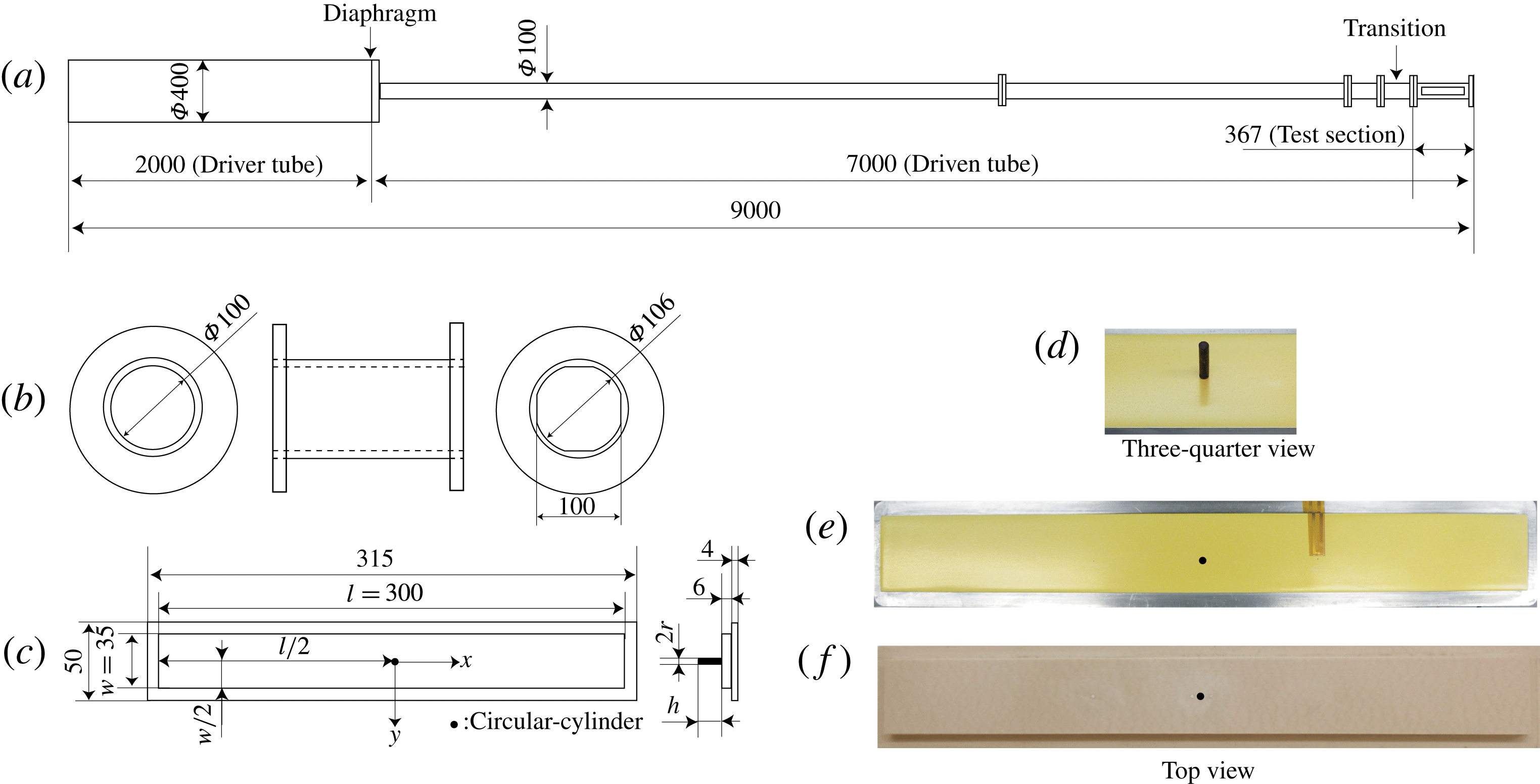
All experiments in the present study were conducted in the shock-tube facility at the Tokyo Metropolitan University (TMU); detailed schematics of the facility are shown in figure 2. This facility is a convergent type of shock tube, with the driver tube having a larger diameter than the driven tube (Resler, Lin & Kantrowitz Reference Resler, Lin and Kantrowitz1952; Alpher & White Reference Alpher and White1958). In general, a range of flow conditions are achievable in shock tubes through varying the driver/driven tube pressures and gas compositions, and potentially the temperatures; here, both sections were unheated and air was used as both the driver and driven gas, leaving the driver pressure,
 $p_{4}$
, and the driven pressure,
 $p_{1}$
, as the two parameters that could be varied. Our interest here was in the aerothermal phenomena induced by a SWBLI, necessitating a sufficiently strong shock to generate a supersonic post-shock flow. As an air driver is limited in its ability to produce strong shocks, it was decided to keep the shock and post-shock Mach numbers fixed, and to vary the post-shock unit Reynolds number. This was achieved by varying
 $p_{4}$
and
 $p_{1}$
individually while keeping the ratio
 $p_{4}/p_{1}$
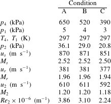
fixed at a value of 130. Three conditions were explored, denoted by A, B and C:
 $p_{4}=650~\text{kPa}$
and
 $p_{1}=5~\text{kPa}$
for condition A,
 $520~\text{kPa}$
and
 $4~\text{kPa}$
for condition B,
 $390~\text{kPa}$
and
 $3~\text{kPa}$
for condition C. Inviscid one-dimensional theory for this pressure ratio and choice of gases predicts an incident shock speed of
 $u_{s}=965~\text{m}~\text{s}^{-1}$
(
 $M_{s}=2.8$
), a reflected shock speed of
 $u_{r}=404~\text{m}~\text{s}^{-1}$
(
 $M_{r}=2.0$
relative to the post-incident-shock flow), and a useful test time of approximately 1.0 ms at the upstream end of the test section. Here, the subscripts
 $s$
and
 $r$
denote the incident shock and the reflected shock wave, respectively. The actual test conditions as calculated from measured pressure records will be presented shortly.
(a–c) Schematics of the shock tube (a), transition piece (b), flat-plate test article (c); (d–f) photographs of the circular cylinder (d), the flat plate with a TSP coating (e) and with a mounted thermocouple (f).

As shown in figure 2, the test section had an octagonal cross-section (to simplify optical access), with the internal distance between opposite sides equal to the internal diameter of the upstream circular section (
 $100~\text{mm}$
). The cross-sectional area in the test section was therefore slightly (8 %) larger. The changeover from the circular to the octagonal cross-section took place at the transition piece, indicated in figure 2.
Theoretical flow conditions were verified by means of pressure measurements on the shock-tube wall. Two fast-response PCB sensors (model 113B26) were installed at
 $x=-60~\text{mm}$
and
 $x=0$
(the origin of the coordinate system used here is the location of the centre of the cylindrical obstacle to be discussed shortly), allowing both pressure variations and shock speeds to be measured. The sensor outputs were recorded at
 $1~\text{MHz}$
using a Dewetron data acquisition system. Static pressure variations for the three test conditions measured at
 $x=-60~\text{mm}$
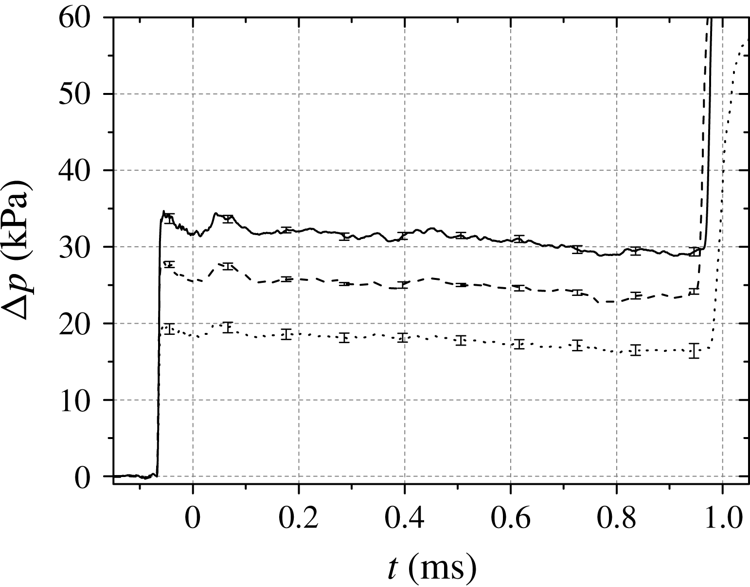
are presented in figure 3. The plotted profiles represent ensemble-averaged data over six shots in each case, with error bars indicating the standard deviation within each set (typically less than 5 %). The pressure increases from the incident and reflected shock waves are clearly visible: for condition A, the pressure rise induced by the incident shock is approximately
 $35~\text{kPa}$
and the time-averaged pressure rise in the interval between the incident-shock and reflected-shock arrivals is
 $31.1~\text{kPa}$
. This compares with the predicted theoretical increase from inviscid one-dimensional theory of
 $40~\text{kPa}$
. This discrepancy can be attributed to three factors: (1) the increase in cross-sectional area at the transition piece, (2) shock attenuation caused by viscous effects in the driven tube (Mirels Reference Mirels1957), and (3) boundary-layer growth behind the incident shock. The first two of these factors will contribute solely to a lower initial pressure rise, while the third will also cause the decreasing pressure trend after shock arrival. The standard deviation in the time interval between the incident-shock and reflected-shock arrivals at
 $x=-60~\text{mm}$
over the six shots for each condition was less than 1 % in each case. This delay between incident and reflected shocks resulted in a representative test time at
 $x=-60~\text{mm}$
for all cases of approximately
 $1~\text{ms}$
.
Pressure variations at
 $x=-60~\text{mm}$
on the flat plate: ——, Condition A; – –, Condition B;
 $\cdots \cdots$
, Condition C. The error bars indicate the standard deviation over six repeated shots in each case.

The flow characteristics for the three test conditions are summarized in table 1. Representative conditions behind the incident shock (subscript 2) as well as the shock speed itself (
 $u_{s}$
) were estimated from the average measured pressures between incident and reflected shocks using the normal shock relations. The incident shock speed derived in this manner showed good agreement with that estimated from the time elapsed between the shock arrivals at the two PCB sensors (
 $873\pm 26~\text{m}~\text{s}^{-1}$
).
Summary of the experimental conditions used in this study. The subscripts 1, 4 and 2 refer to conditions in the driver section, in the driven section, and behind the incident shock; subscripts
 $s$
and
 $r$
refer to the incident and reflected shocks.

Four of the test-section walls (at
 $90^{\circ }$
intervals) contained cavities in which an optical window or an instrumentation insert/test article could be installed. Three insert types were used in separate experiments, each consisting of a flat plate with a circular cylinder attached: (i) a quartz insert to allow plan-view schlieren images to be recorded; (ii) a polyurethane-coated aluminium insert for TSP measurements; (iii) an insert constructed of polyether ether ketone (PEEK) with coaxial thermocouples installed (Medtherm E-type, TCS-061,
 $1.6~\text{mm}$
diameter). Because of manufacturing tolerances, there was a backward-facing step of
 $170\pm 1.1~\unicode[STIX]{x03BC}\text{m}$
height at the intersection between the shock-tube wall and the inserts. The circular cylinder was mounted at the centrepoint of the flat plate, which will be taken as the origin for the coordinate system to be used throughout this paper (with
 $x$
representing the streamwise direction and
 $y$
the lateral direction in the plane of the flat-plate surface). The axis of the cylinder was normal to the flat-plate surface (see figure 2). The cylinder radius,
 $r$
, was
 $1.5~\text{mm}$
in all cases; two different heights were selected based on boundary-layer calculations to be described in § 3.1, namely
 $h=5.5~\text{mm}$
and
 $15.0~\text{mm}$
(i.e.
 $h/r=3.7$
and 10.0). The larger height was chosen such that the top of the cylinder would remain outside the boundary layer throughout the test time for all conditions, while the smaller height was chosen so that the cylinder would become submerged within the boundary-layer flow. The coaxial thermocouple locations in relevant experiments were
 $x/r=-2.3$
and 3.3 with
 $y/r=0$
. The pre-shock wall temperature for TSP experiments was recorded using a sheet-shaped K-type thermocouple, mounted at
 $x/r=33.3$
. This thermocouple had a thickness of
 $0.7~\text{mm}$
and was attached by a 0.05-mm-thick Kapton film.
2.2 TSP methodology
The implementation of TSP in this study followed that of the first author’s previous work (Ozawa Reference Ozawa2016). The aluminium insert was first covered with a 100-
 $\unicode[STIX]{x03BC}\text{m}$
thick insulating layer of white polyurethane (PUR). PUR has a comparatively low thermal conductivity, and thus experiences large temperature variations at the surface. The white colour results in a high reflectance, increasing the effective emission of the TSP directed to the imaging device. The TSP was of the binder type, consisting of a dichlorotris (1,10-phenanthroline) ruthenium (II) hydrate (98 %) luminophore (Ruphen) with an ethanol-soluble polyamide-based polymer serving as the binder. The TSP was applied directly to the PUR base layer using a spray gun. Ruphen has a short luminescent lifetime of less than
 $1~\unicode[STIX]{x03BC}\text{s}$
(Mills Reference Mills1997) and an absorption peak at
 $\unicode[STIX]{x1D706}_{ab}=450~\text{nm}$
, readily accessible by commercially available blue light-emitting diodes (LED). The maximum emission occurs at
 $\unicode[STIX]{x1D706}_{em}=580~\text{nm}$
, enabling any reflected light at the excitation wavelength to be filtered out. The thickness of the applied TSP layer was estimated using a film thickness meter (VL-50-B, Mitutoyo) as
 $1.5~\unicode[STIX]{x03BC}\text{m}\pm 0.5~\unicode[STIX]{x03BC}\text{m}$
. The circular cylinder was painted black to minimize reflections; it was attached to the flat-plate model following application of the TSP layer.
Temperature and pressure calibrations of the employed TSP were carried out using a
 $10\times 10$
-mm TSP sample in a calibration chamber that was controllable to within
 $0.1~\text{K}$
and
 $0.1~\text{kPa}$
. The temperature was increased from
 $253~\text{K}$
to
 $368~\text{K}$
in 5 K temperature steps at
 $100~\text{kPa}$
, and the pressure was varied between
 $100~\text{kPa}$
,
 $80~\text{kPa}$
,
 $50~\text{kPa}$
and
 $20~\text{kPa}$
at
 $293~\text{K}$
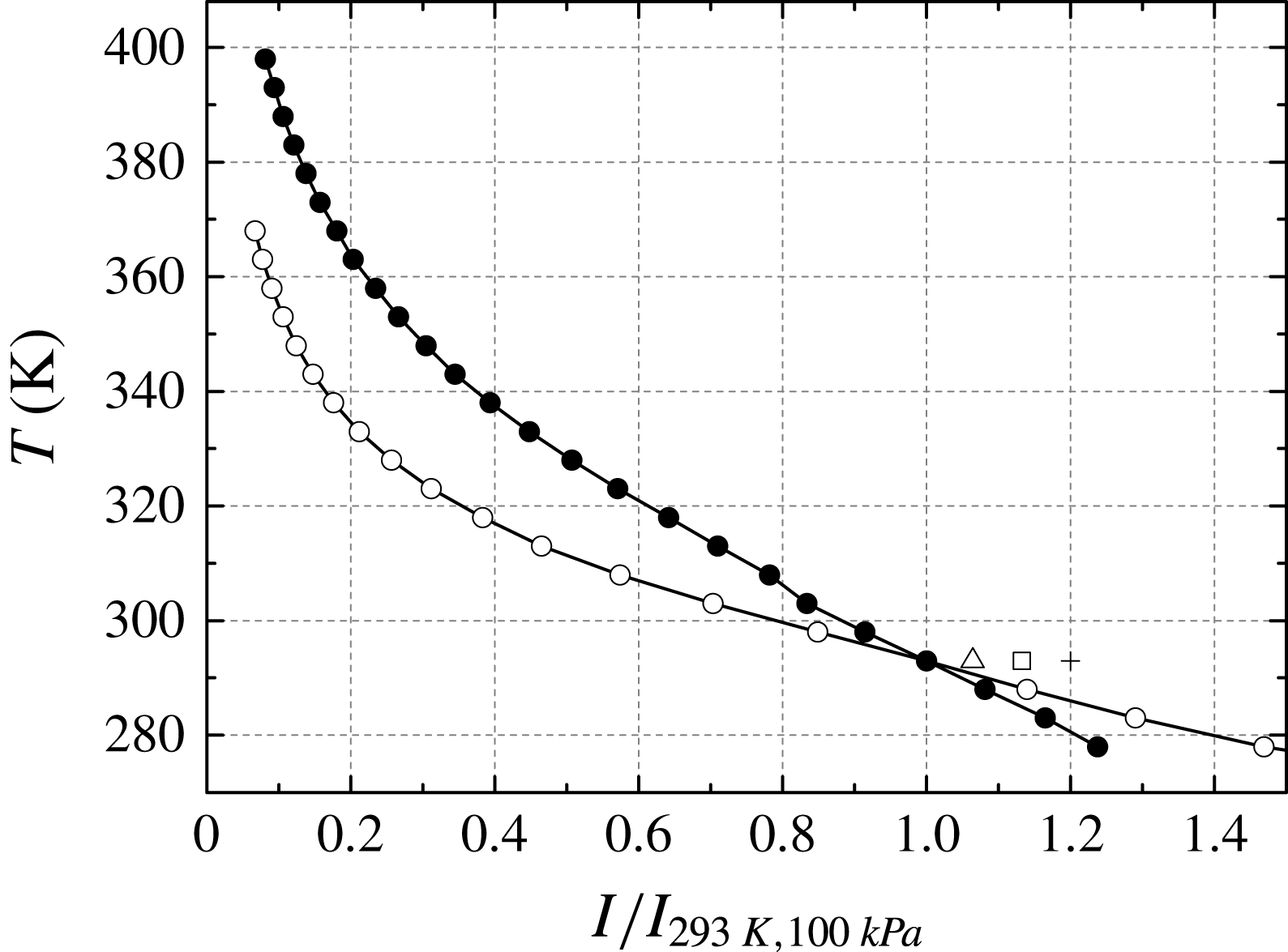
. Figure 4 shows the intensity-temperature calibration data, together with the ninth-order polynomial curve that was used to convert the intensity to temperature in practice. The use of a ninth-order curve was justified in that a higher-order polynomial fit resulted in a negligible change in the derived heat flux. Also shown in figure 4 is the calibration curve for the Ruphen-based TSP used in previous work (Martinez Schramm et al.
Reference Martinez Schramm, Hannemann, Ozawa, Beck and Klein2015; Ozawa et al.
Reference Ozawa, Laurence, Martinez Schramm, Wagner and Hannemann2015), which employed an acryl-based polymer binder. The temperature sensitivity of the current TSP at
 $293~\text{K}$
is above
 $-4\,\%~\text{K}^{-1}$
, significantly higher than the previous formulation. In prior experiments on a flat plate without a cylinder (Ozawa Reference Ozawa2016), temperature rises as high as
 $10~\text{K}$
above ambient were observed; with the higher heat fluxes expected for the SWBLI in the present experiments, intensity changes above 50 % were expected.
Plots of calibrated temperature versus normalized intensity: —
 $\bullet$
—, earlier TSP formulation used in Ozawa (Reference Ozawa2016); —
 $\circ$
—, present formulation at
 $100~\text{kPa}$
; ▵, ▫, +, present formulation at
 $80~\text{kPa}$
,
 $50~\text{kPa}$
and
 $20~\text{kPa}$
, respectively.

Figure 4 also shows the employed TSP to have non-negligible pressure sensitivity, with the normalized intensity ratio at
 $80~\text{kPa}$
and
 $293~\text{K}$
being 6 % higher than at
 $100~\text{kPa}$
, for example. Note, however, that a typical polymer has an oxygen diffusion coefficient,
 $\unicode[STIX]{x1D6FC}_{d}$
, of the order of
 $10^{-9}~\text{m}^{2}~\text{s}^{-1}$
(Kameda et al.
Reference Kameda, Seki, Makoshi, Amao and Nakakita2012), which is two orders of magnitude smaller than the thermal diffusivity of the polymer used in this study. This means that the characteristic response time for pressure changes will be of the order of a hundred times longer than that for changes in temperature. We can characterize this difference more concretely in terms of penetration depth. For a step change in oxygen concentration at the surface, the depth at which the concentration falls to 50 % of the surface value after
 $0.1~\text{ms}$
(characteristic of the relevant time scales in the present experiments) can be calculated by solving the one-dimensional diffusion equation as approximately
 $0.3~\unicode[STIX]{x03BC}\text{m}$
(assuming
 $\unicode[STIX]{x1D6FC}_{d}=1\times 10^{-9}~\text{m}^{2}~\text{s}^{-1}$
). For a step change in heat flux, the corresponding penetration depth can be determined from the one-dimensional solution provided by Schultz & Jones (Reference Schultz and Jones1973) as
 $2~\unicode[STIX]{x03BC}\text{m}$
(using the value of thermal diffusivity,
 $\unicode[STIX]{x1D6FC}_{p}$
, given below). Considering the thickness of the TSP layer (
 $1.5~\unicode[STIX]{x03BC}\text{m}$
), we conclude that the effect of the pressure sensitivity on the emission intensity will be small in the present experiments.
In order to derive the heat flux from temperature measurements, knowledge of the thermal properties of both the base layer (which can be considered semi-infinite over the time scales of interest here) and the TSP layer is required. Measurements of the PUR base-layer material and polyamide-based polymer were performed by an external company, Japan Fine Ceramics Center (JFCC). The specific heat,
 $c$
, and thermal diffusivity,
 $\unicode[STIX]{x1D6FC}$
, were measured using differential scanning calorimetry and the laser flash method, respectively. The thermal properties of PUR with associated uncertainties were
 $\unicode[STIX]{x1D70C}_{b}=1.167\times 10^{3}~\text{kg}~\text{m}^{-3}\pm 10\,\%$
,
 $c_{b}=1.59~\text{kJ}~\text{kg}^{-1}~\text{K}^{-1}\pm 3\,\%$
and
 $\unicode[STIX]{x1D6FC}_{b}=1.09\times 10^{-7}~\text{m}^{2}~\text{s}^{-1}\pm 7\,\%$
as reported by Ozawa et al. (Reference Ozawa, Laurence, Martinez Schramm, Wagner and Hannemann2015), whereas those of the polyamide-based polymer were
 $\unicode[STIX]{x1D70C}_{p}=1.132\times 10^{3}~\text{kg}~\text{m}^{-3}\pm 10\,\%$
,
 $c_{p}=2.07~\text{kJ}~\text{kg}^{-1}~\text{K}^{-1}\pm 3\,\%$
and
 $\unicode[STIX]{x1D6FC}_{p}=0.84\times 10^{-7}~\text{m}^{2}~\text{s}^{-1}\pm 7\,\%$
. Here,
 $\unicode[STIX]{x1D70C}$
is the material density, and the subscripts
 $b$
and
 $p$
denote the base layer and the polymer layer.
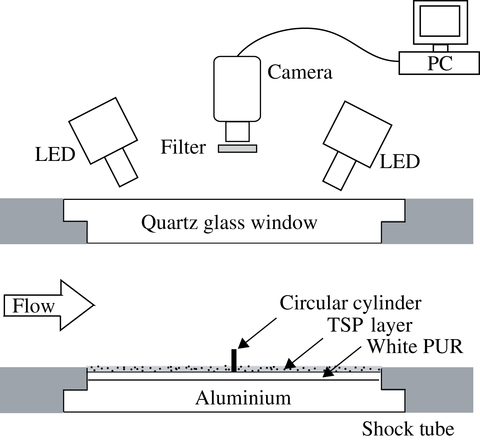
Schematic of optical set-up for TSP measurement and installation of the flat-plate test article with circular cylinder.

The optical set-up for the TSP measurements is shown in figure 5. Two identical LED light sources manufactured by Luminus, Inc. were equipped with collecting lenses and used to excite the TSP dye. The LEDs were operated continuously with a driver current of
 $24~\text{A}$
for a duration of 1 second during each experiment to minimize degradation of the TSP. Their excitation wavelength was
 $\unicode[STIX]{x1D706}_{ex}=462~\text{nm}$
, with a full-width at half-maximum of
 $22~\text{nm}$
. A Phantom v2011 was employed as the detector in this experiment, allowing high-speed 12-bit recording. A sampling frequency of
 $180~\text{kHz}$
with an exposure time of
 $3.86~\unicode[STIX]{x03BC}\text{s}$
was typically used, which allowed a visualization area of
 $384\times 204$
pixels, corresponding to a physical area of
 $44.2~\text{mm}\times 23.5~\text{mm}$
(i.e.
 $0.115~\text{mm}~\text{pixel}^{-1}$
). The 3.0-mm diameter of the circular cylinder was then represented by 26 pixels. A bandpass filter placed in front of the high-speed camera allowed wavelengths of
 $560{-}640~\text{nm}$
(compared to the TSP emission peak of
 $580~\text{nm}$
) to pass with a transmission ratio of more than 90 %.
In order to derive the heat-flux profiles that will be presented throughout this paper, the following procedure was employed. Each image in a recorded sequence was first normalized by a reference, flow-off image, to obtain the normalized intensity,
 $I/I_{norm}$
. These normalized intensities were then transformed into temperature maps by means of the calibration curve shown in figure 4. Temperature histories at individual locations were then extracted and converted into time-resolved heat-flux curves by means of the algorithm proposed by Liu et al. (Reference Liu, Cai, Lai, Rubal and Sullivan2010), an adaptation of an earlier routine by Cook & Felderman (Reference Cook and Felderman1966) taking into account the finite TSP-layer thickness. Temporal smoothing was applied to increase the signal-to-noise ratio, with 5- and 3-point moving average filters applied to the temperature and heat-flux histories; spatial filtering over a
 $5\times 5$
pixel window was also applied for curves extracted at particular locations (but not distributions). This level of filtering was chosen subjectively as a compromise between minimizing measurement noise while maintaining adequate temporal response: the effect of the temporal filtering is to increase the effective rise time (5 % to 95 %) for the TSP-based heat-flux measurement to approximately
 $30~\unicode[STIX]{x03BC}\text{s}$
. In an earlier work (Ozawa et al.
Reference Ozawa, Laurence, Martinez Schramm, Wagner and Hannemann2015), the uncertainty in heat flux derived from a similar Ruphen-based TSP was estimated to be 16 %; this was dominated primarily by uncertainties in the thermal properties of the base layer and in the intensity–temperature calibration. Since the base-layer material and calibration procedure are identical in the present study, we assume a similar uncertainty, though note that additional error sources may become important during highly transient events (e.g. passage of shocks); in particular, the method for accounting for the finite TSP-layer thickness becomes increasingly approximate as the surface heat flux changes more rapidly.
2.3 Other measurement techniques
Additional pointwise heat-flux measurements were performed using thermocouples (Medtherm type-E coaxial) installed in the PEEK insert, in separate experiments from the TSP tests. The thermocouple outputs were recorded at
 $1~\text{MHz}$
using the same Dewetron data acquisition system as for the facility pressure measurements. The response time of the thermocouples is less than
 $1~\unicode[STIX]{x03BC}\text{s}$
. Heat-flux histories were derived using the numerical algorithm of Cook & Felderman (Reference Cook and Felderman1966). Moving average filters of 29 points were used to smooth both temperature and heat-flux profiles obtained from the thermocouples, increasing the effective rise time of the thermocouple-based heat-flux measurement to approximately
 $40~\unicode[STIX]{x03BC}\text{s}$
(comparable to that of the TSP). The minimum uncertainty in thermocouple-derived heat-flux measurements is estimated as approximately 10 %, contributed to primarily by uncertainty in the effective thermal properties.
High-speed schlieren visualization was enabled by replacing the opaque inserts with quartz glass inserts, on one of which the cylinder was attached. This enabled plan-view visualizations of the unsteady shock structures generated by the interaction of the supersonic flow with the circular cylinder (side-view visualization not being possible due to the constraints of the octagonal test section). A continuous LED light source was employed as the light source, while images were recorded by the same Phantom v2011 camera as used in the TSP experiments. The frame rate was again
 $180~\text{kHz}$
with an exposure time of
 $3.86~\unicode[STIX]{x03BC}\text{s}$
. The image resolution employed was
 $384\times 204$
pixels which, with a magnification of
 $0.090~\text{mm}~\text{pixel}^{-1}$
, allowed a visualization area of
 $34.8~\text{mm}\times 18.5~\text{mm}$
. The imaged cylinder diameter was then 33 pixels.
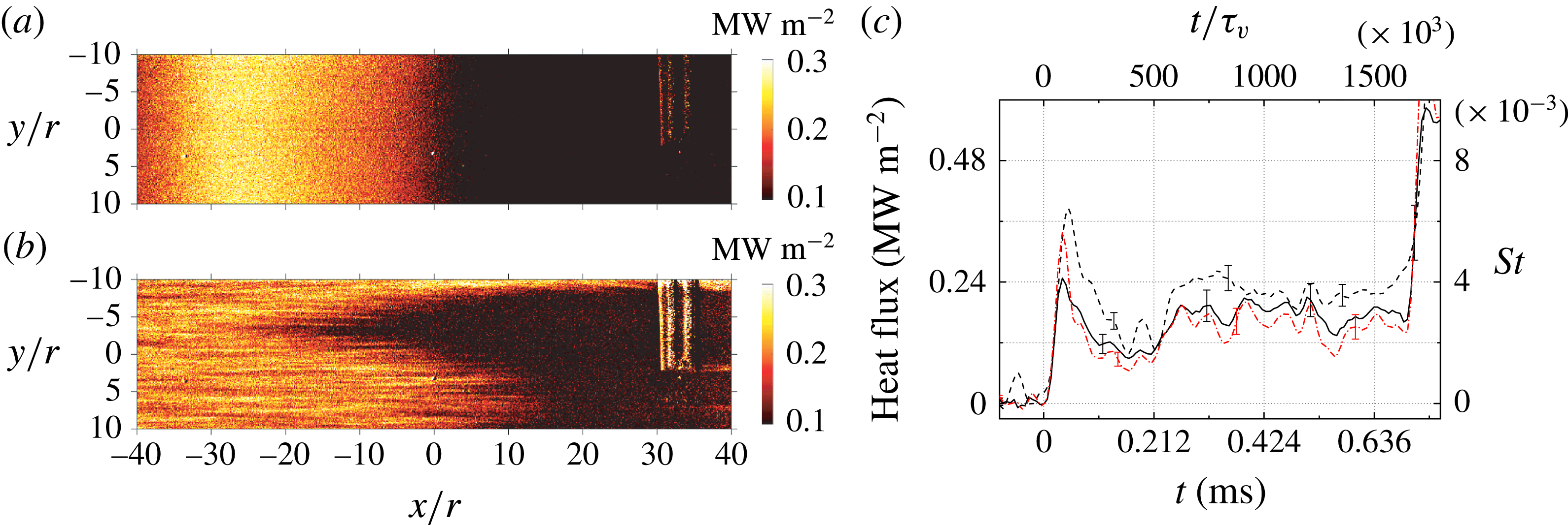
(a,b) Instantaneous heat-flux distributions on the flat plate without the cylinder: (a) incident shock passage at
 $t=0$
; (b) arrival of the laminar-to-turbulent transition front at
 $t=0.214~\text{ms}$
. (c) Time-resolved heat-flux record at
 $x=0$
,
 $y=0$
as measured by: – –, thermocouple; ——, TSP (previous result by Ozawa (Reference Ozawa2016)); – ⋅ – ⋅ –, TSP (present result).

3 Results and discussion
3.1 Shock-tube wall flow and theoretical boundary-layer thickness for a flat plate
We first consider the basic boundary-layer flow over the flat plate in the absence of the circular cylinder. A detailed investigation of this problem was conducted using the TSP technique in an earlier work by the first author (Ozawa Reference Ozawa2016). Representative results in figure 6 show instantaneous heat-flux distributions on the flat plate for condition A, corresponding to the arrival first of the incident shock and then the transition front
 $0.214~\text{ms}$
later. Note that the present TSP results are derived using the algorithm of Liu et al. (Reference Liu, Cai, Lai, Rubal and Sullivan2010), whereas in the earlier work the numerical procedure of Cook & Felderman (Reference Cook and Felderman1966), which ignores the finite TSP-layer thickness, was employed. Plotted in the right part of figure 6(
 $c$
) are the time-resolved heat fluxes derived from both TSP and a thermocouple at a location corresponding to
 $x=y=0$
in the present experiments. The shock arrival time here is at
 $t=0$
. Error bars indicate the experimental uncertainties in each technique referred to in the previous section. A second temporal scaling, in which the physical time is normalized by a viscous time scale, is indicated on the upper axis; more will be said about this shortly. TSP profiles calculated using both the Cook & Felderman (Reference Cook and Felderman1966) and Liu et al. (Reference Liu, Cai, Lai, Rubal and Sullivan2010) algorithms are presented. The Liu et al. algorithm is expected to be more accurate at short time scales, and indeed, improved agreement with the thermocouple signal immediately upon shock arrival (i.e. the initial peak) is observed compared to the Cook & Felderman algorithm, with slightly lower readings thereafter. Both show a relatively lower heat flux at later times compared to the thermocouple; however, this generally lies within the experimental uncertainty (including shot-to-shot variation). The onset of transition is clearly visible from the rise in heat flux at
 $t=0.214~\text{ms}$
, and the still larger rise at
 $t\approx 0.7~\text{ms}$
corresponds to the arrival of the reflected shock.
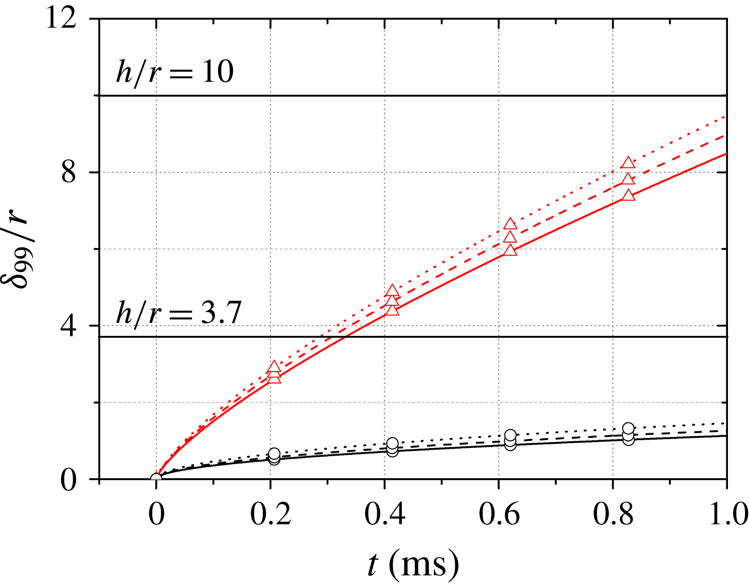
Estimates of boundary-layer heights versus time, with the two cylinder heights indicated: ——, Condition A; – – –, Condition B;
 $\cdots \cdots$
, Condition C. The boundary-layer state is indicated by: ○, laminar; ▵, turbulent.

In this study, two cylinder heights were chosen based on theoretical estimates of the boundary-layer thickness on the shock-tube wall during the available test time. In particular, it was desired to have cases both in which the cylinder height remained larger than boundary-layer thickness throughout the test time and in which the cylinder became submerged within the boundary layer. Figure 7 shows the temporal development of the boundary-layer thickness at
 $x=0$
on the flat plate for the three test conditions. The laminar profiles were calculated according to the theory of Mirels (Reference Mirels1955) while the turbulent profiles are based on the estimates of Martin (Reference Martin1958). Both
 $1/7$
and
 $1/5$
power laws have been proposed for the turbulent boundary-layer growth on a shock-tube wall (Mirels Reference Mirels1955; Martin Reference Martin1958). Using experimental interferometry data, Martin (Reference Martin1958) reported improved agreement with the
 $1/5$
power law compared to the
 $1/7$
power law; as condition A in the present study is very similar to the test condition in Martin’s work, the
 $1/5$
power law was considered here. In any case, the turbulent profiles plotted in figure 7 should be considered estimates rather than precise values, especially considering the flow is laminar for a significant period of time (the transition time varied from
 ${\sim}0.2~\text{ms}$
for Condition A to
 ${\sim}0.3~\text{ms}$
for Condition C). According to these predictions, we expect that for all conditions the top of the larger cylinder will remain outside the boundary layer throughout the test time, whereas the smaller cylinder will become submerged within the boundary layer. It should be noted here that it did prove challenging to obtain repeatable transition Reynolds numbers between tests (the relevant Reynolds number here being
 $\unicode[STIX]{x1D70C}_{2}u_{2}^{2}t/\unicode[STIX]{x1D707}_{2}$
, with
 $\unicode[STIX]{x1D707}_{2}$
the post-shock coefficient of viscosity – see Mirels Reference Mirels1955), even at the same nominal test condition. Such difficulties have been noted by earlier researchers in similar experiments (Thompson & Emrich Reference Thompson and Emrich1967; Brun Reference Brun1985), and are likely associated with the difficulty of ensuring the shock-tube wall surface was completely clean. The shock-tube wall and especially the TSP surface were cleaned using an air duster before each experiment to remove any obvious particulate matter (and particularly diaphragm fragments), but it is likely that some small roughness elements remained and affected the transition behaviour.
3.2 Circular cylinder,
 $h/r=10$

3.2.1 General two-dimensional flow phenomena
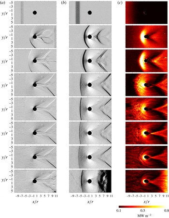
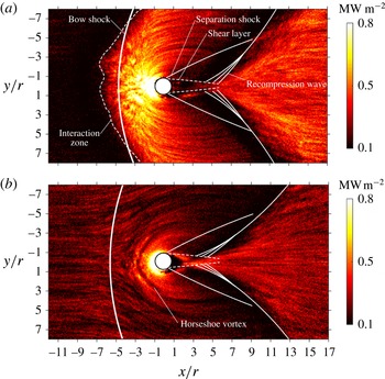
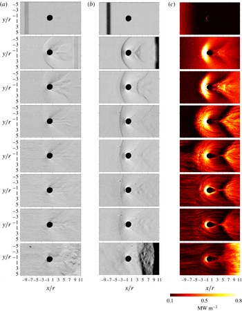
In figure 8 we present a sequence of time-resolved schlieren images and corresponding TSP-derived heat-flux distributions for the case of Condition A with the 15-mm cylinder. As the various sequences were recorded in different experiments, the experimental times have been synchronized by means of the pressure measurements discussed earlier. Schlieren sequences with both vertical and horizontal knife-edge orientations are shown: the former reveals the presence of the bow shock upstream of the cylinder more readily, while the latter provides improved visualization of the wake phenomena as well as the upstream boundary-layer structures. A movie of the entire sequence with the different visualization types is available as part of the online supplementary material at https://doi.org/10.1017/jfm.2018.433. In figure 9, we have extracted the main flow features from the schlieren images at two time steps (the first in which the incoming boundary layer is laminar, the second in which it is turbulent) and superimposed these on the heat-flux distributions.
Sequences of schlieren images and TSP-derived heat-flux distributions for condition A with
 $h/r=10$
: (a,b) the vertical and horizontal density gradients visualized by schlieren photography; (c) the instantaneous heat flux. The experimental times are (top to bottom)
 $t=-0.006$
, 0.028, 0.044, 0.111, 0.183, 0.228, 0.317 and
 $0.667~\text{ms}$
.

At the first time shown (
 $t=-0.006~\text{ms}$
), the incident shock is visible ahead of the cylinder between
 $x/r=-7$
and
 $-5$
in the schlieren images, and a corresponding increase in heat flux is observed extending to the left of the shock in the TSP visualization. During the subsequent three time steps (
 $t=0.028~\text{ms}$
to
 $t=0.111~\text{ms}$
), the heat-flux distributions show a region of enhanced heating spreading radially outwards from the cylinder as the bow shock develops ahead of the cylinder in the schlieren images. The bow shock appears particularly strong in the vertical knife-edge images during this development, indicating that it is largely two-dimensional at this point. This is to be expected, considering the large aspect ratio of the cylinder and the relatively thin laminar boundary layer, meaning that although a shock-wave/laminar-boundary-layer interaction (SWLBLI) forms near the foot of the cylinder, the majority of the cylinder is exposed to essentially inviscid supersonic flow. The thickening of the upstream boundary layer during this period is evidenced by the decrease in heat flux in the undisturbed region of the flow.
Instantaneous heat-flux distributions with main features from schlieren images overlaid: (a)
 $t=0.111~\text{ms}$
; (b)
 $t=0.317~\text{ms}$
.

The
 $t=0.111~\text{ms}$
snapshot is also reproduced in the upper plot of figure 9, with the key visualized schlieren features superimposed on the heat-flux distribution. The leading edge of the bow shock has propagated upstream to
 $x/r=-5.0$
, whereas the increase in heat flux has already extended as far as
 $x/r=-6.7$
; clearly, the influence of the unsteady SWLBLI on the wall heating extends upstream of the generating shock and, for clarity, we refer to the upstream surface region over which the heat flux is affected by the SWBLI as the ‘interaction zone’. This behaviour is consistent with previous observations of steady SWLBLIs by, for example, Mark (Reference Mark1958) and North & Stuart (Reference North and Stuart1962). Note that unlike earlier steady SWLBLI studies, however, we do not observe a pronounced region of decreased heating at the upstream edge of the interaction. As will be discussed in the following subsection, this is likely an indication that the separated region has not yet been fully established. A number of curved, streak-like features are present in the heat-flux distribution around and upstream of the cylinder in this TSP image and to a lesser extent in the previous one (
 $t=0.044~\text{ms}$
). These streaks resemble the turbulent features seen in previous measurements of the undisturbed flat-plate boundary layer (Ozawa Reference Ozawa2016). We therefore conclude that, by
 $t=0.111~\text{ms}$
, the SWLBLI ahead of the cylinder is inducing laminar-to-turbulent boundary-layer transition immediately downstream of the interaction.
Changing our viewpoint to the wake of the cylinder, details of the corresponding steady flow patterns are found in Sedney & Kitchens (Reference Sedney and Kitchens1975) and may be used as a reference for the present unsteady development. The TSP image at
 $t=0.111~\text{ms}$
shows a fan-shaped region of increased heating with curved sides extending downstream of the cylinder. The schlieren images reveal a shear layer being shed from either side of the rear of the cylinder, with associated separation shocks. The distance between the two shear layers reaches a minimum at the neck region lying at around
 $x/r=5$
, from which point recompression waves are generated. The spatial relationship between these waves and the fan-shaped region is seen clearly in figure 9; considering the close proximity of these features, it is tempting to draw also a causal link. Just upstream of the recompression wave, a notable decrease in heat flux is observed; the heat flux then increases directly behind the recompression to reach a maximum level a short distance downstream.
At
 $t=0.183~\text{ms}$
, the streak-like heat-flux features now appear beneath the incoming flow; furthermore, the corresponding schlieren image shows non-homogeneities in the vertical density gradient in this region. These phenomena indicate the onset of transition in the incoming boundary layer. The arrival of these streaks corresponds to a disruption and partial collapse of the interaction zone ahead of the cylinder, as the bow shock interacts with the transitional, spatially non-uniform incoming boundary layer.
Once transition has occurred and the boundary layer ahead of the cylinder is fully turbulent (
 $t=0.228~\text{ms}$
), the region of severe heating upstream of the cylinder becomes concentrated closely in the vicinity of the cylinder (as far upstream as approximately
 $x/r=-2.1$
); this likely indicates a diminishing of the separation zone in the SWTBLI compared to the SWLBLI, consistent with the steady results of Hung & Clauss (Reference Hung and Clauss1981). As for the heat flux behind the cylinder, we note from the TSP images that the fan-shaped region has become sharper and narrower, and its origin on the centreline has moved upstream in the cylinder wake following transition. We refer to this origin as the ‘apex’. Initially (
 $t=0.111~\text{ms}$
), the apex seems to lie at the neck region; however, it is a surface heat-flux feature rather than an inviscid flow feature, and therefore does not necessarily correspond directly to the neck region visualized in the schlieren images. In fact, in contrast to the TSP distributions, the wake region in the schlieren images shows relatively little variation as the incoming boundary-layer transitions to turbulence – primarily just a slight decrease in the recompression wave angle from
 ${\sim}46^{\circ }$
at
 $t=0.111~\text{ms}$
to
 ${\sim}42^{\circ }$
at
 $t=0.228~\text{ms}$
. This motivates separate terminology for the neck region and apex. At
 $x/r=3.0$
,
 $t=0.228~\text{ms}$
, particularly severe heating is seen at the apex. Comparing with the surface flow sketches of Sedney & Kitchens (Reference Sedney and Kitchens1975), the apex location coincides approximately with the unstable node on the flow symmetry plane (which is also an attachment line for large protuberances).
At
 $t=0.317~\text{ms}$
(also shown in figure 9), the global heat-flux level has decreased compared to the previous TSP-derived image. At this time, the turbulent boundary-layer thickness has grown to the order of
 $\unicode[STIX]{x1D6FF}/r=3.6$
according to the estimate in figure 7, and the decreasing temperature gradient near the wall thus results in smaller heat fluxes throughout the flow field. The effect of the SWTBLI on the upstream flow field at this time can be delineated by changes in direction of the streaks in the TSP image; these deviate from horizontal between approximately
 $x/r=-8.0$
and
 $x/r=-7.0$
, slightly upstream of the schlieren shock location at approximately
 $x/r=-6.0$
. A notable feature in the heat-flux distribution is a narrow, bow-shaped structure ahead of the cylinder (
 $x/r\gtrsim -3.0$
), which probably reveals the presence of a horseshoe vortex; in particular, this is reminiscent of the four- or six-vortex configuration sketched in figure 11 of Sedney & Kitchens (Reference Sedney and Kitchens1975). These earlier authors reported that the number of vortices within the separated region ahead of the cylinder in steady flow decreases as the Reynolds number is increased. Even at
 $t=0.667~\text{ms}$
, however, just before the arrival of the reflected shock, the bow-shaped heat-flux feature ahead of the cylinder is clearly visible.
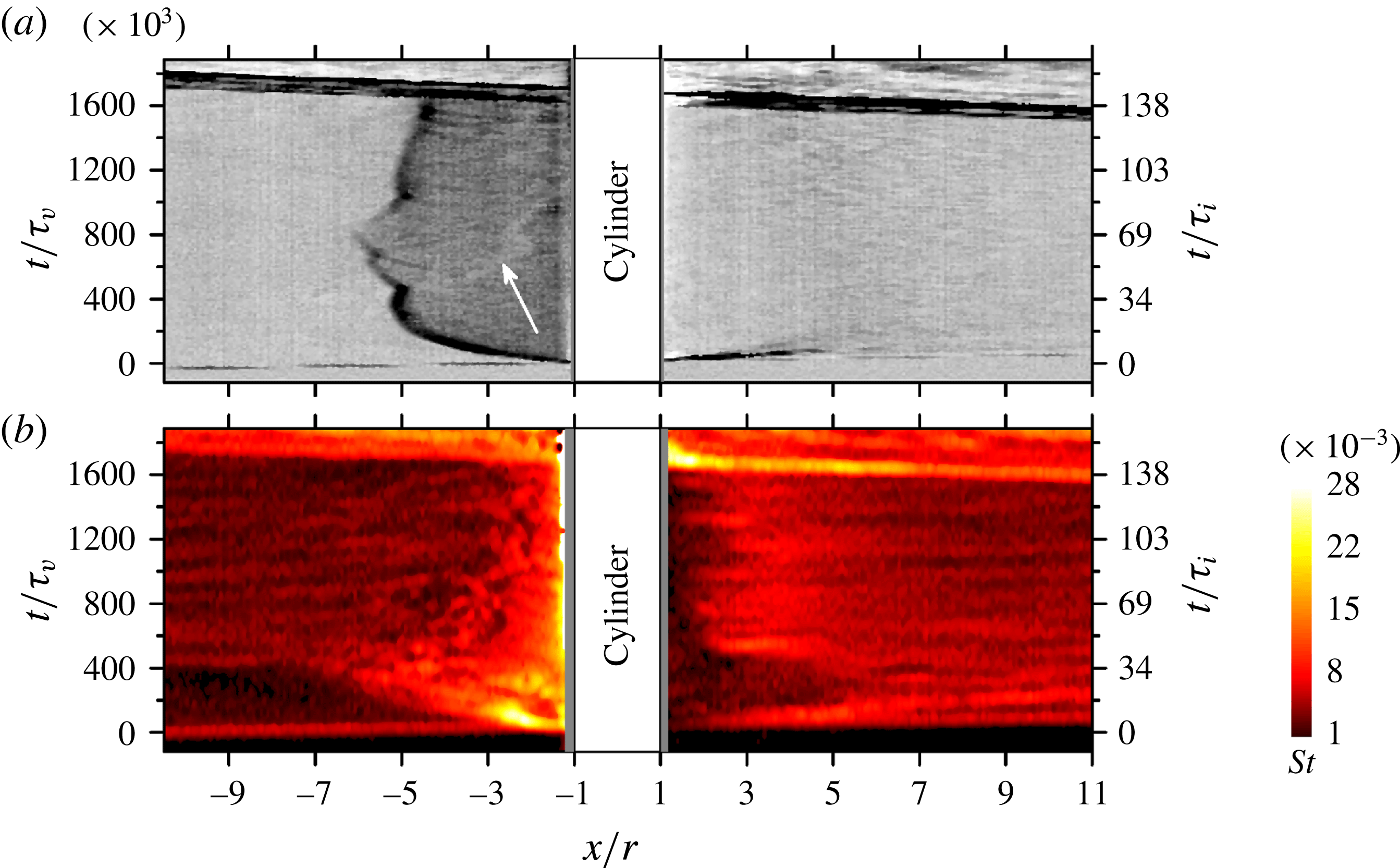
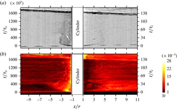
Experimental
 $x$
–
 $t$
diagrams of the horizontal density gradient (a) and Stanton number (b) as measured along the centreline (
 $y=0$
) for Condition A,
 $h/r=10$
.

3.2.2 Detailed unsteady flow development
By extracting measurement points along a line of constant
 $y$
in sequences of schlieren or heat-flux images, we are able to construct
 $x$
–
 $t$
diagrams, a tool often used to depict flow phenomena in shock tubes. Figure 10 shows such
 $x$
–
 $t$
diagrams derived from both schlieren images and Stanton number (
 $St$
) distributions along the line
 $y=0$
for condition-A experiments with
 $h/r=10$
; depicting the development in this way allows a direct comparison of the shock motion ahead of the cylinder with the development of the heat flux on the flat-plate surface. The Stanton number is defined here as
 $$\begin{eqnarray}\displaystyle & \displaystyle St={\displaystyle \frac{q_{w}}{\unicode[STIX]{x1D70C}_{2}u_{2}c_{p}(T_{2r}-T_{w})}}, & \displaystyle\end{eqnarray}$$
where
 $q_{w}$
is the heat flux at the wall,
 $c_{p}$
is the specific heat at constant pressure,
 $T_{2r}$
is the laminar recovery temperature and
 $T_{w}$
is the wall temperature. In figure 11, the Stanton number
 $x$
–
 $t$
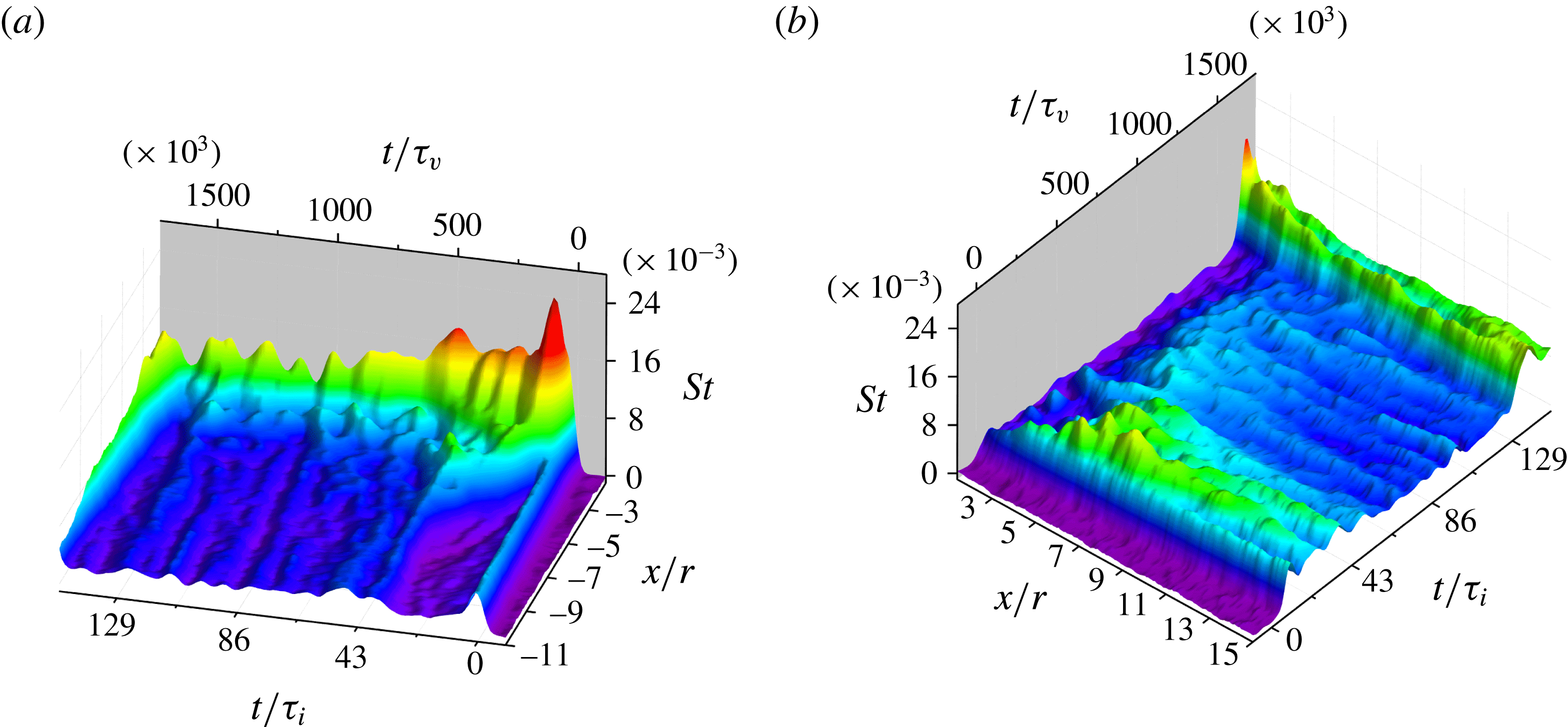
diagram has been recast as two contour plots showing the regions fore and aft of the cylinder separately, allowing a clearer picture of the quantitative heating levels. In both figures 10 and 11, two scalings for the time axis are shown: one in which the normalization is through the viscous time scale
 $\unicode[STIX]{x1D70F}_{v}=\unicode[STIX]{x1D707}_{2}/(\unicode[STIX]{x1D70C}_{2}u_{2}^{2})$
(
 $=4.2\times 10^{-10}~\text{s}$
for condition A); the other employing the inviscid time scale
 $\unicode[STIX]{x1D70F}_{i}=r/u_{2}$
(
 $=4.9~\unicode[STIX]{x03BC}\text{s}$
to
 $5.0~\unicode[STIX]{x03BC}\text{s}$
for all conditions). The former scaling (
 $t/\unicode[STIX]{x1D70F}_{v}$
) can be interpreted as the Reynolds number of the incoming boundary layer (Mirels Reference Mirels1955), while the latter is the relevant time scale for the development of the inviscid flow features away from the wall.
In figure 10 we clearly see the initial upstream motion of the bow shock ahead of the cylinder in the schlieren-derived
 $x$
–
 $t$
diagram and a corresponding growth of the interaction zone in the TSP-derived diagram. The motion of the interaction-zone boundary continues steadily upstream even after the shock-wave propagation has paused at
 $x/r=-5.3$
,
 $t/\unicode[STIX]{x1D70F}_{v}=380\times 10^{3}$
. The interaction zone reaches as far as approximately
 $x/r=-6.7$
at
 $t/\unicode[STIX]{x1D70F}_{v}=432\times 10^{3}$
, at which point the streaks indicating transition to turbulence of the incoming boundary layer arrive from upstream. This suggests that the separated flow region ahead of the shock is still developing when the boundary-layer transitions, which is not surprising considering the longer establishment times required for separated versus non-separated flows (Holden Reference Holden1971). This may also explain the absence of a clear decrease in heat flux upstream of the shock position, which would be expected in the case of a steady laminar SWBLI. The collapse of the interaction zone back towards the cylinder following the arrival of the turbulent streaks is readily apparent in the TSP diagram. The schlieren-derived diagram shows a corresponding feature (indicated by an arrow) which may be associated with the retreating of the Mach stem, since separation structures would not be expected to appear in schlieren images. The maximum Stanton number that occurs during the flow development just described is
 $St=25.3\times 10^{-3}$
– equivalent to
 $1.53~\text{MW}~\text{m}^{-2}$
– at
 $x/r=-2.1$
,
 $t/\unicode[STIX]{x1D70F}_{v}=78\times 10^{3}$
; i.e. the severest heating appeared during the early motion of the shock and growth of the interaction zone upstream.
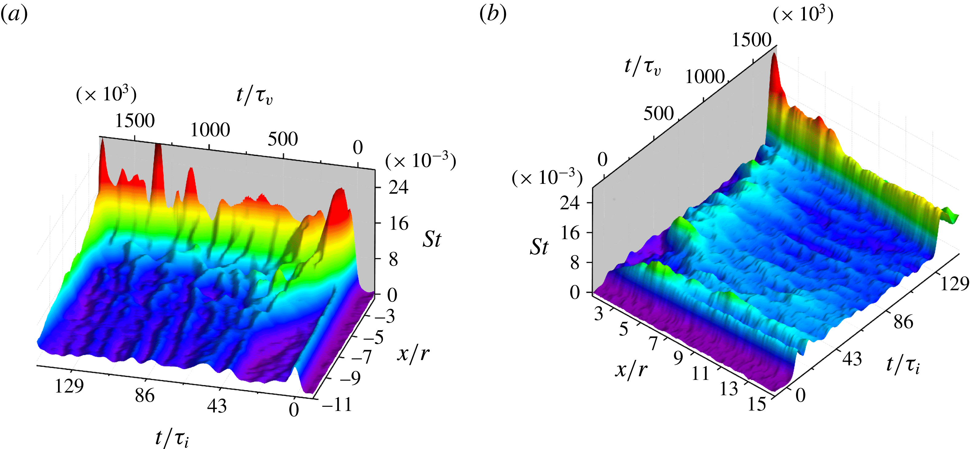
Surface contour plots in
 $x$
–
 $t$
space of the Stanton number along the centreline (a) upstream and (b) downstream of the cylinder for Condition A,
 $h/r=10$
.

Estruch (Reference Estruch2016) showed that the peak surface heating upstream of a blunt obstacle in hypersonic flow could be correlated with (and was of the same order as) the stagnation-point heating on the obstacle. Here, we can estimate this stagnation-point heating as (see White Reference White1991)
 $$\begin{eqnarray}\displaystyle & \displaystyle q_{0}=0.570Pr^{-0.6}\sqrt{\unicode[STIX]{x1D70C}_{e}\unicode[STIX]{x1D707}_{e}K}\left({\displaystyle \frac{\unicode[STIX]{x1D70C}_{w}\unicode[STIX]{x1D707}_{w}}{\unicode[STIX]{x1D70C}_{e}\unicode[STIX]{x1D707}_{e}}}\right)^{0.1}(h_{e}-h_{w}), & \displaystyle\end{eqnarray}$$
where
 $Pr$
is the Prandtl number,
 $h$
is the static enthalpy, and subscripts
 $e$
and
 $w$
refer to conditions at the boundary-layer edge (i.e. the inviscid stagnation conditions behind the bow shock) and the cylinder wall, respectively. The velocity gradient,
 $K$
, may be approximated as
 $$\begin{eqnarray}\displaystyle & \displaystyle K={\displaystyle \frac{\text{d}u_{e}}{\text{d}s}}\approx {\displaystyle \frac{u_{2}}{r}}\sqrt{2{\displaystyle \frac{\unicode[STIX]{x1D70C}_{2}}{\unicode[STIX]{x1D70C}_{e}}}}, & \displaystyle\end{eqnarray}$$
where
 $s$
represents the distance along the cylinder wall from the stagnation point (or line). The latter approximation makes use of Newtonian impact theory, which is most suitable for hypersonic Mach numbers; nevertheless, White (Reference White1991) shows that it remains a reasonable approximation even for low supersonic Mach numbers. In the present case (Condition A), equations (3.2) and (3.3) predict a stagnation heating value of
 $q_{0}=0.98~\text{MW}~\text{m}^{-2}$
. We see then that the maximum heating level on the wall surface during the upstream shock motion exceeds this value by more than 50 %.
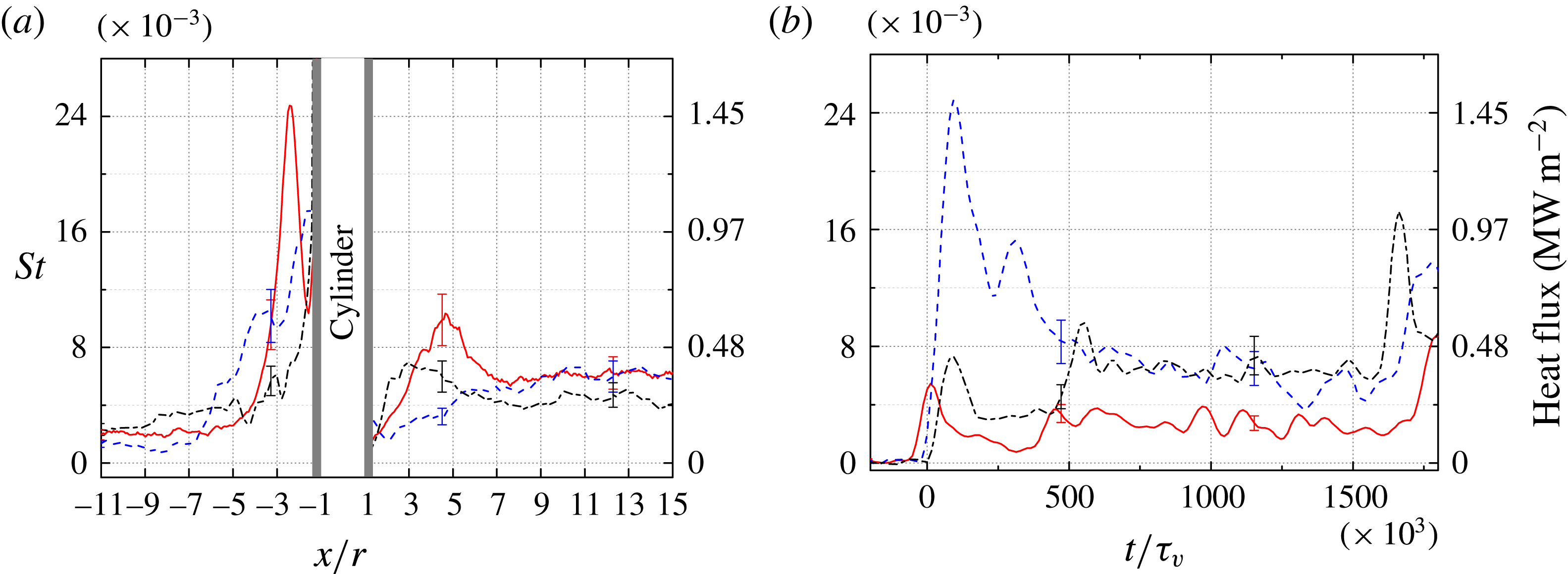
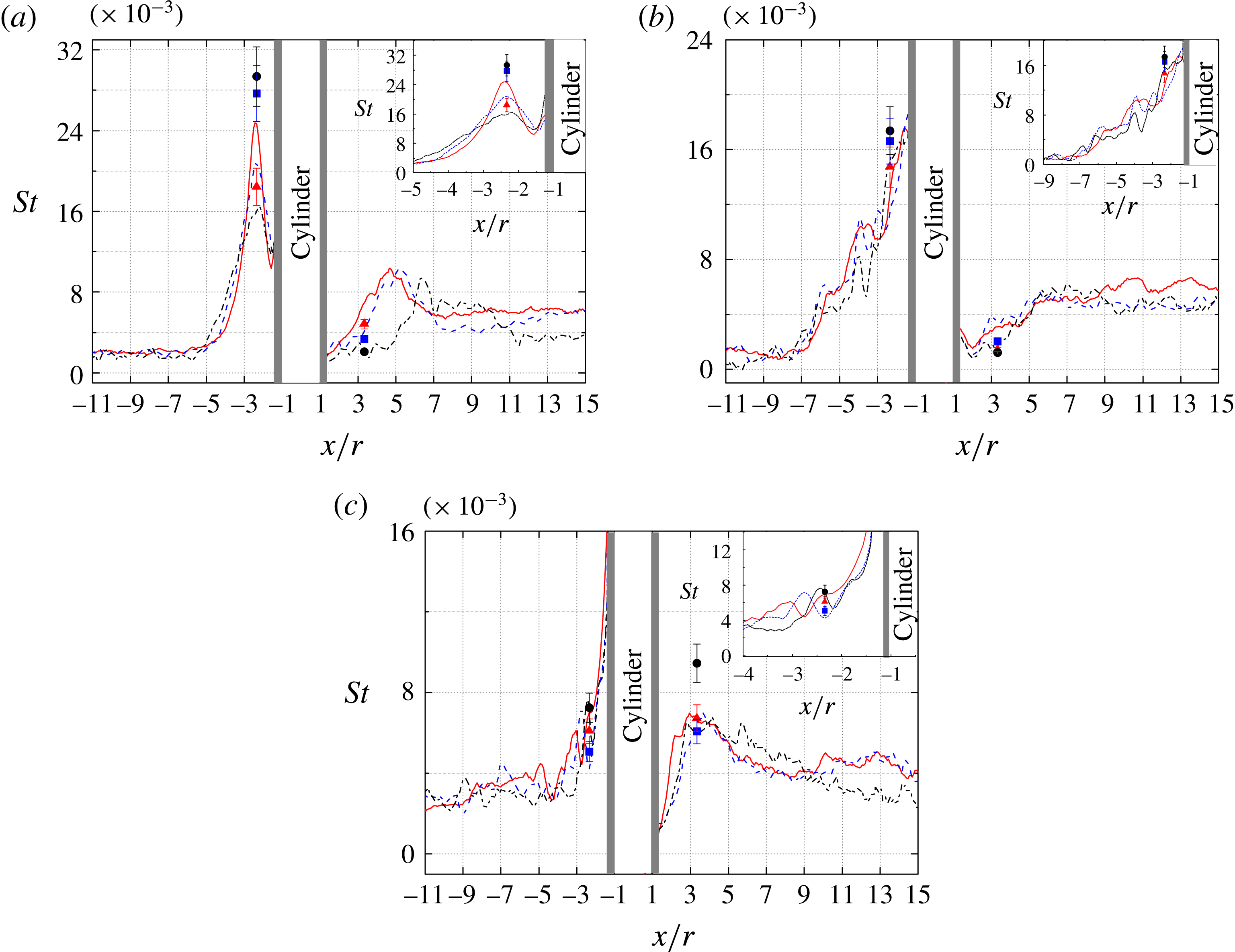
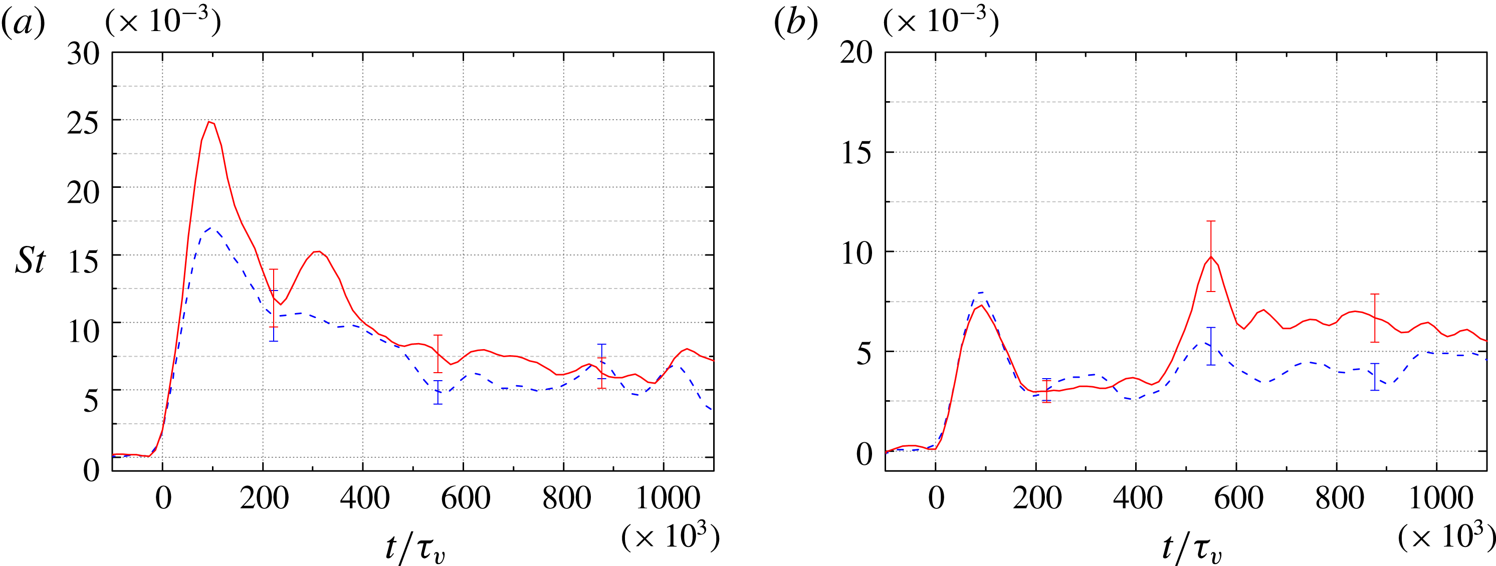
To aid us in further analysing the flow development upstream of the cylinder, in figure 12 we have extracted and plotted the Stanton number along the centreline at three instants in time, as well as at three points along the centreline as functions of time (these points were chosen to match the locations of thermocouple measurements to be discussed shortly). Representative error bars are also included at certain points on these plots. Looking first to the distribution along the centreline at
 $t/\unicode[STIX]{x1D70F}_{v}=105\times 10^{3}$
(a), the Stanton number increases steeply from
 $x/r\approx -3.3$
as a result of the SWLBLI, reaches a sharp maximum, and thereafter decreases rapidly just ahead of the cylinder. At the next time shown,
 $t/\unicode[STIX]{x1D70F}_{v}=262\times 10^{3}$
, the upstream heat flux has decreased as the laminar boundary layer has thickened, and the interaction zone has extended further upstream with the peak heat flux now directly at the base of the cylinder. At
 $t/\unicode[STIX]{x1D70F}_{v}=746\times 10^{3}$
, the incoming boundary layer has transitioned to turbulence, leading to increased heating upstream of the interaction zone, but the region of SWBLI-enhanced heat flux has withdrawn downstream, beginning from approximately
 $x/r=-4$
and rising even more sharply to its peak at the cylinder base. Some small localized peaks in the streamwise Stanton number appear in this curve, for instance, at
 $x/r=-3.3$
. This peak corresponds to the bow-shaped feature suggested earlier to be the signature of a horseshoe vortex, and indeed, such localized humps in heat flux were interpreted by Hung & Clauss (Reference Hung and Clauss1981) as corresponding to separation and reattachment of secondary vortical structures. By comparing with figure 11, however, we conclude that most such peaks in the present case are transient and thus probably not associated with vortices (with the exception of that just mentioned).
(a) Instantaneous Stanton number profiles along the centreline for Condition A,
 $h/r=10$
, at times: ——,
 $t=0.043~\text{ms}$
(
 $t/\unicode[STIX]{x1D70F}_{v}=105\times 10^{3}$
); – –,
 $t=0.111~\text{ms}$
(
 $t/\unicode[STIX]{x1D70F}_{v}=262\times 10^{3}$
); – ⋅ – ⋅ –,
 $t=0.317~\text{ms}$
(
 $t/\unicode[STIX]{x1D70F}_{v}=746\times 10^{3}$
). (b) Time-resolved Stanton number curves at individual locations along the centreline: ——,
 $x/r=-10.0$
; – –,
 $x/r=-2.3$
; – ⋅ – ⋅ –,
 $x/r=3.3$
.

Looking now to the Stanton number time record at
 $x/r=-2.3$
(figure 12
b), the heat load first increases with the passage of the incident shock, followed by a more drastic rise caused by the SWLBLI – these two events are not resolvable from one another at this
 $x/r$
location, but the more limited rise caused by the incident shock alone may be seen in the
 $x/r=-10.0$
curve, which exhibits a heat-flux history very similar to the basic flat-plate flow shown in figure 6. A rapid drop in
 $St$
follows thereafter with some fluctuations superimposed. These fluctuations are caused primarily by disturbances propagating from upstream – the turbulent streaks noted earlier – the trajectories in
 $x$
–
 $t$
space of which can be seen clearly in figure 11(a). These disturbances also appear to be responsible for the large-scale peaks and troughs visible in the peak heating region close to the base of the cylinder in this plot.
Shifting our focus now to the cylinder wake, an
 $x$
–
 $t$
diagram of the Stanton number along the centreline behind the cylinder is shown in figure 11(b), and the temporal development at a single point (
 $x/r=3.3$
) is included in figure 12(b). The Stanton number remains relatively small in the wake immediately downstream of the cylinder following the passage of the incident shock; in this area we expect the formation of a reverse flow region and possibly a counter-rotating vortex pair (Sedney & Kitchens Reference Sedney and Kitchens1975). The extent of this reduced heat flux region (which may delineate the reversed flow region, since reattachment generally leads to increased heat flux) decreases after transition to turbulence of the incoming boundary layer. Further elucidation of the intricate wake-flow structures is difficult with the present techniques.
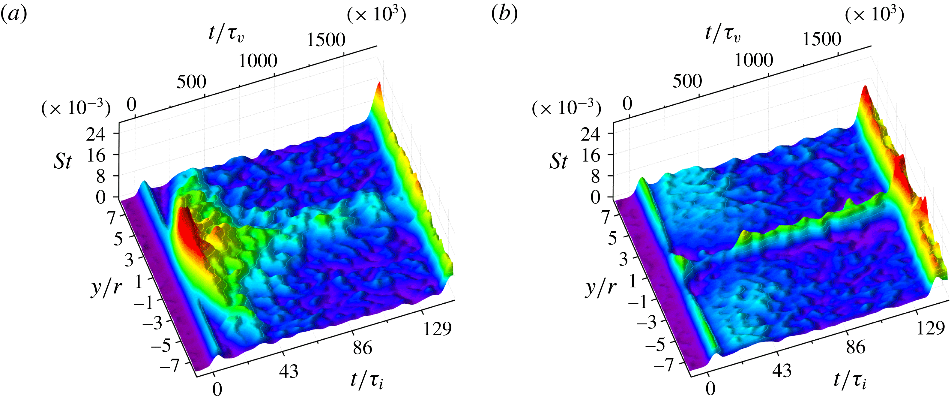
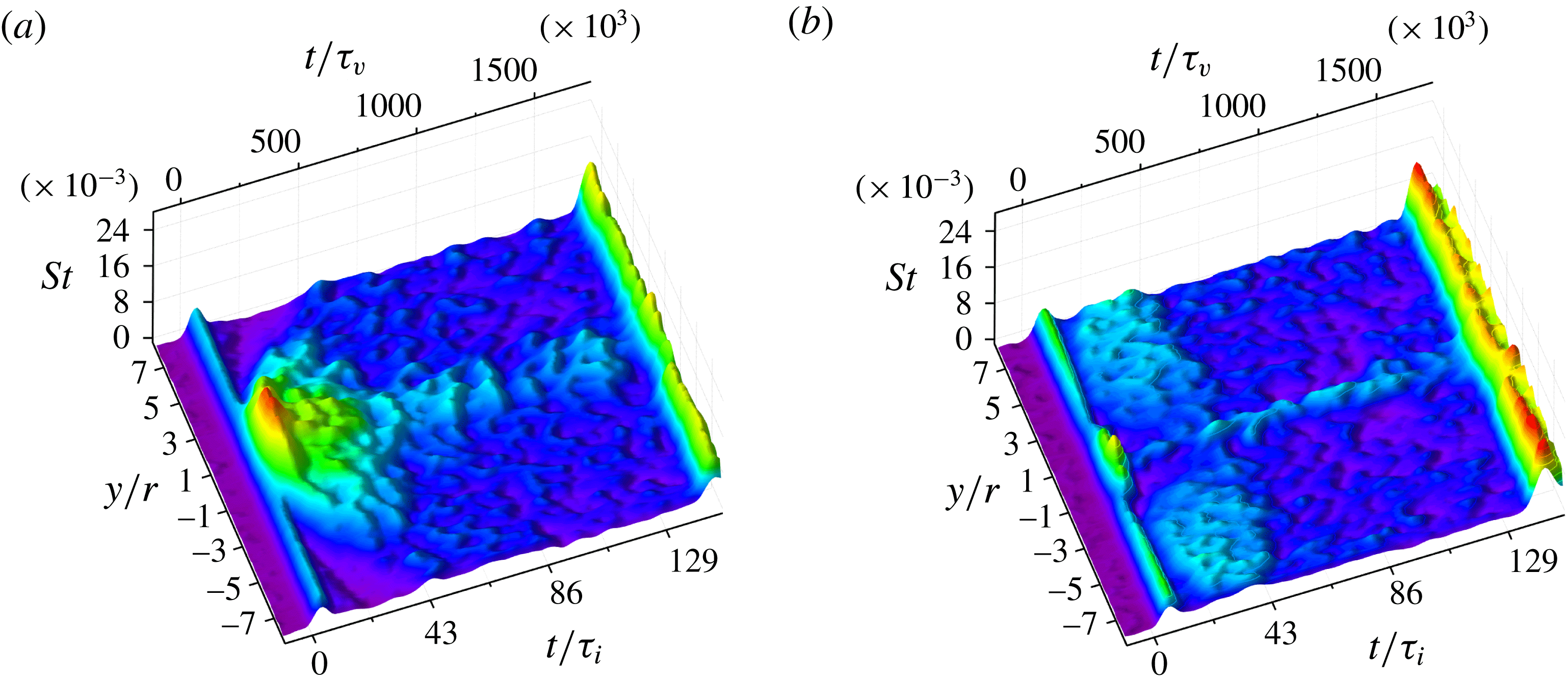
Surface contour plots of the Stanton number in
 $y$
–
 $t$
space at (a)
 $x/r=-2.3$
and (b)
 $x/r=3.3$
for Condition A,
 $h/r=10$
.

Figure 13 shows contour plots of the Stanton number versus
 $y/r$
and
 $t$
, extracted at
 $x/r=-2.3$
and 3.3. In the upstream plot (figure 13
a), following the passage of the incident shock at
 $t/\unicode[STIX]{x1D70F}_{v}=-26\times 10^{3}$
, the Stanton number increases drastically and the lateral extent of the interaction zone grows rapidly. This pattern ends abruptly at approximately
 $t/\unicode[STIX]{x1D70F}_{v}=250\times 10^{3}$
, with the interaction zone taking on a much less uniform appearance; this behaviour coincides with the flow in this region becoming transitional (though the incoming boundary layer remains laminar), as indicated by the local appearance of streaks in figure 8. Following transition to turbulence of the incoming boundary layer at approximately
 $t/\unicode[STIX]{x1D70F}_{v}=420\times 10^{3}$
, the interaction zone decreases in lateral extent and the peak heating diminishes until the arrival of the reflected shock. In the downstream plot (figure 13
b), the Stanton number increases only mildly with the passage of the incident shock, and during the time the incoming boundary layer is laminar, the heating levels across the depicted region remain modest. Once transition occurs, however, we observe the onset of high heating over a narrow region about the apex; this persists at approximately the same level until the reflected shock arrives.
3.2.3 Effect of varying the unit Reynolds number
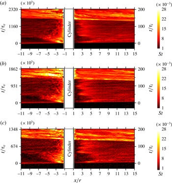
Further experiments were carried out at the other two unit Reynolds number conditions summarized in table 1. Movies of the time-resolved Stanton number distributions for all conditions (and for both cylinder heights) are included in the online supplementary material. In figure 14 we present Stanton number
 $x$
–
 $t$
diagrams along the centreline for the three different conditions, all with
 $h/r=10$
. The experimental time has been normalized by both the viscous (left axes) and inviscid (right axes) time scales, with the inviscid scaling being common between the three plots. As noted earlier, it was difficult to achieve consistent transition Reynolds numbers of the incoming boundary layer even for experiments with the same test conditions; the three experiments presented here were chosen based on their exhibiting a similar transition Reynolds number (
 $t/\unicode[STIX]{x1D70F}_{v}$
). The three pictures share largely similar qualitative features, though differences are observed in the timing of these. The initial development of the upstream interaction region as the bow shock propagates forward appears to agree well between the three conditions if the inviscid scaling is used. This scaling, however, clearly fails to collapse the onset of turbulence of the incoming boundary layer (which is to be expected given the criterion for selecting the experiments); similarly, the timing of the wake development in the three cases shows clear differences with the
 $t/\unicode[STIX]{x1D70F}_{i}$
normalization.
Experimentally derived
 $x$
–
 $t$
diagrams of the Stanton number along the centreline with
 $h/r=10$
for (a–c) conditions A to C, respectively.

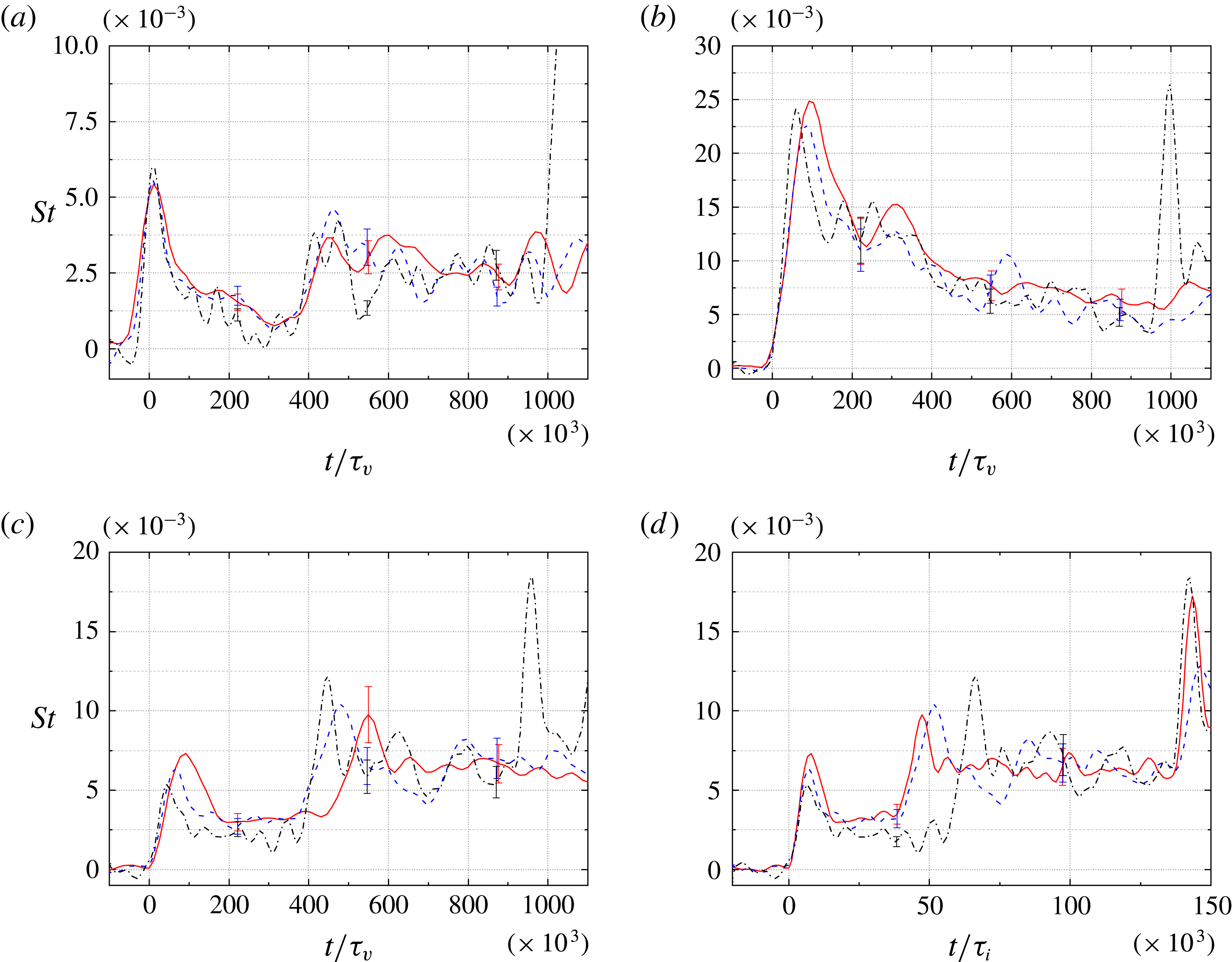
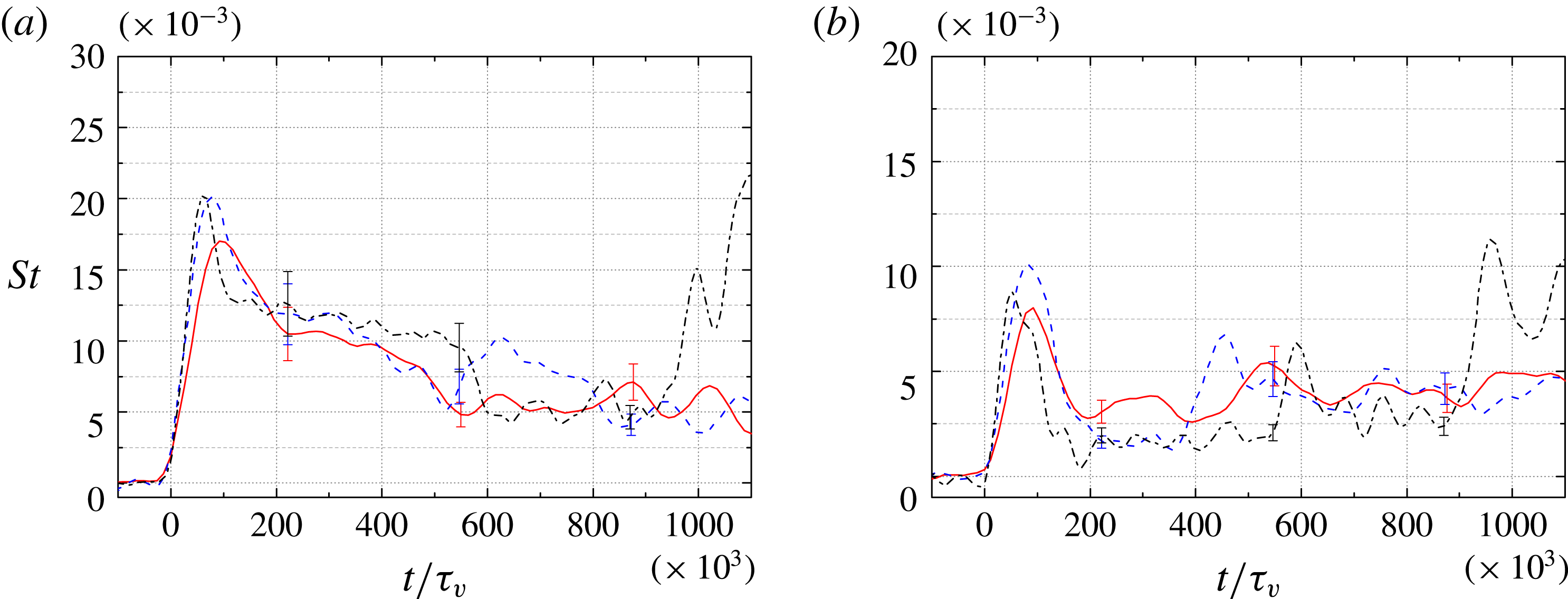
Time-resolved Stanton number curves for
 $h/r=10$
at the following locations along the centreline: (a)
 $x/r=-10.0$
; (b)
 $x/r=-2.3$
; (c,d)
 $x/r=3.3$
. In each plot, the different curves correspond to: ——, Condition A; – –, Condition B; – ⋅ – ⋅ –, Condition C. Panel (d) uses the inviscid normalization; all others use the viscous normalization.

To identify such differences more precisely, in figure 15 we present temporally developing Stanton number curves at three points along the centreline for the three conditions. In figure 15(a), for which
 $x/r=-10.0$
(i.e. upstream of the influence of the cylinder), we see that the
 $t/\unicode[STIX]{x1D70F}_{v}$
-
 $St$
scaling does an admirable job of collapsing the curves onto one another, both in terms of the timing of transition to turbulence (which again is to be expected) and in the magnitude of the Stanton number throughout. Some minor differences are present, particularly associated with the unsteady streaks following transition, but we conclude that the
 $t/\unicode[STIX]{x1D70F}_{v}$
scaling is appropriate for this undisturbed boundary-layer flow. At
 $x/r=-2.3$
(figure 15
b), i.e. just upstream of the cylinder, we note first a small discrepancy in the timing of the peaks corresponding to the arrival of the upstream-propagating bow shock with the viscous scaling; this could be anticipated considering that the inviscid scaling is more appropriate during this initial phase. Shortly thereafter, however, the curves follow one another relatively closely until the arrival of the reflected shock in the Condition-C trace. This would suggest that, except for the initial bow shock propagation, the flow development in the region upstream of the cylinder is primarily dominated by viscous effects, i.e. the establishment of the separated region and its scaling with the upstream boundary layer. Looking now at figure 15(c,d), we see that the
 $t/\unicode[STIX]{x1D70F}_{v}$
scaling does a poorer overall job than the
 $t/\unicode[STIX]{x1D70F}_{i}$
scaling of collapsing the three curves in the wake region (
 $x/r=3.3$
), indicating that the inviscid, external time scale is important here. Holden (Reference Holden1971) was similarly able to collapse the flow establishment time for the base flow of spheres using a scaling based on the free-stream velocity and sphere diameter, equivalent to the inviscid scaling employed here; the establishment time for the external base flow is somewhat larger than that required to establish the upstream, unseparated external flow, which would explain the differing behaviours in the upstream and downstream regions observed here.
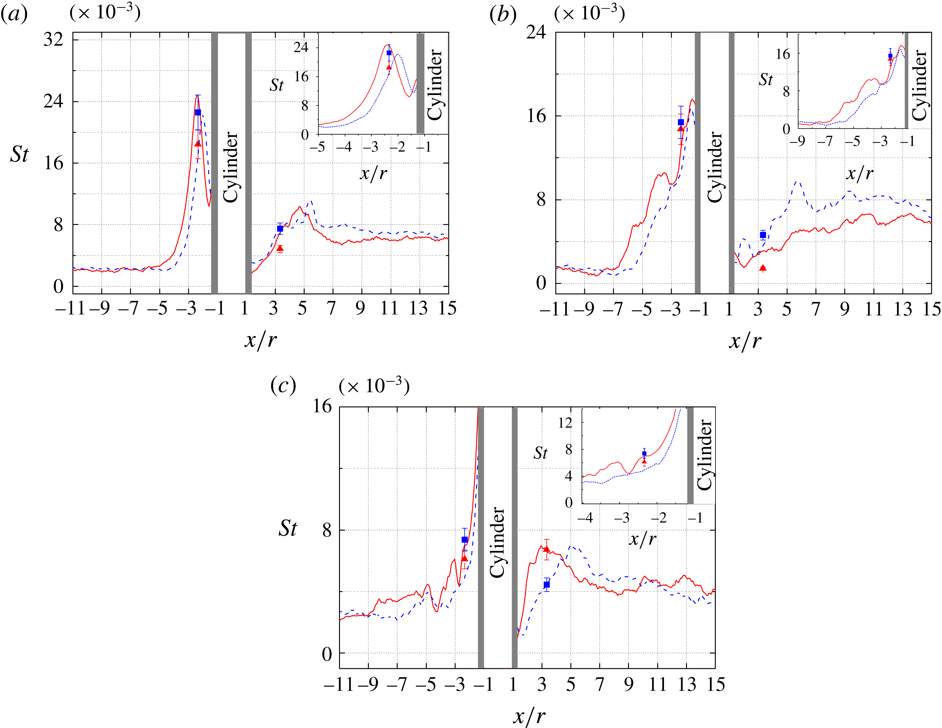
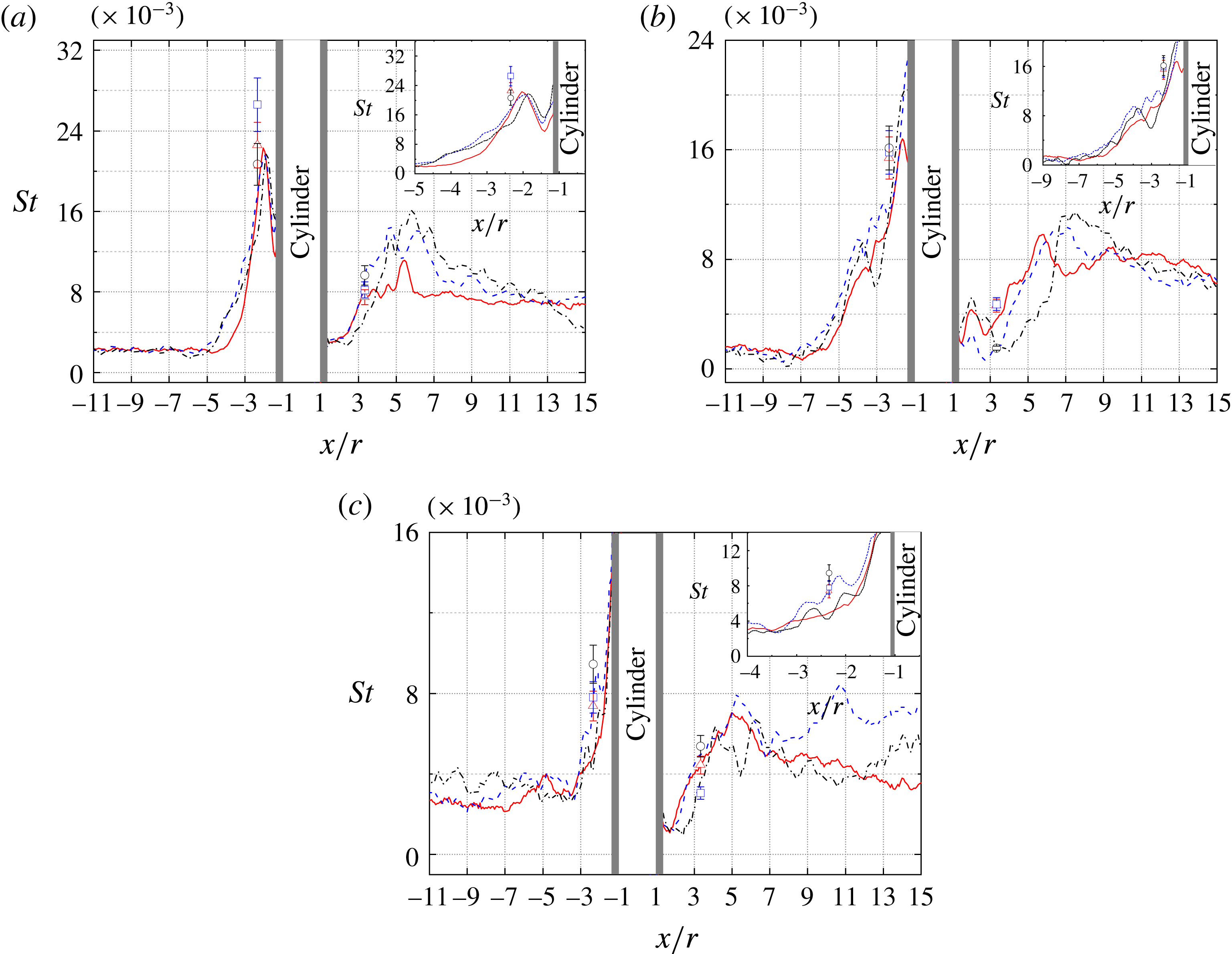
Instantaneous Stanton number profiles along the centreline for
 $h/r=10.0$
at times: (a)
 $t/\unicode[STIX]{x1D70F}_{v}=105\times 10^{3}$
; (b)
 $t/\unicode[STIX]{x1D70F}_{v}=262\times 10^{3}$
; (c)
 $t/\unicode[STIX]{x1D70F}_{v}=746\times 10^{3}$
. In each plot, the individual lines correspond to: ——, Condition A; – –, Condition B; – ⋅ – ⋅ –, Condition C. The symbols correspond to instantaneous thermocouple measurements at the relevant times: ▴, Condition A; ▪, Condition B; ●, Condition C.

Finally, in figure 16 we compare the Stanton number profiles along the centreline for the three different conditions at three values of
 $t/\unicode[STIX]{x1D70F}_{v}$
:
 $105\times 10^{3}$
,
 $262\times 10^{3}$
and
 $746\times 10^{3}$
. In these plots we have also included a comparison with the available thermocouple-based results. At
 $t/\unicode[STIX]{x1D70F}_{v}=105\times 10^{3}$
, the TSP curves show reasonable agreement with one another upstream of the cylinder and somewhat poorer agreement downstream; as we observed earlier, the
 $t/\unicode[STIX]{x1D70F}_{v}$
scaling is not entirely appropriate at this point in the flow development in either region. Compared to the thermocouple measurements, the TSP-derived Stanton numbers at
 $x/r=-2.3$
for the lower two unit Reynolds numbers are somewhat underpredicted. This may be partially a result of the spatial filtering in the TSP results; the Condition-A peak, for example, was reduced by approximately 9 % by this filtering. Whatever the cause, our earlier estimates for the peak surface heating during the flow development are likely lower than the true values. At the downstream location (
 $x/r=3.3$
), where the heat flux changes less rapidly with time, the thermocouple and TSP data show better agreement. At
 $t/\unicode[STIX]{x1D70F}_{v}=262\times 10^{3}$
, the upstream TSP curves collapse well, with the Stanton number increasing rapidly towards the cylinder and reaching approximately the same value in all cases. The thermocouple and TSP data show overall acceptable agreement, with any discrepancies reasonably attributable to flow unsteadiness and shot-to-shot variation. Similar comments apply to the upstream parts of the curves at
 $t/\unicode[STIX]{x1D70F}_{v}=746\times 10^{3}$
, when the incoming flow is fully turbulent in all cases. Now we also observe a distinctive hump in each of the curves between
 $x/r=-3$
and
 $-2$
(see inset); this feature was noted earlier in comments on figure 12 and attributed to a secondary horseshoe vortex. The consistency with which this feature appears across the different conditions suggests it indeed to be physical. As the unit Reynolds number is increased, this peak shifts forward and decreases in height. Such behaviour would be consistent with the steady data of Sedney & Kitchens (Reference Sedney and Kitchens1975), in which the general trend was for both the separation and attachment points to move gradually upstream with increasing Reynolds number. Some caution should be exercised in our interpretation here, however, as the corresponding movies reveal that the location of this feature is somewhat unsteady. We also note the contrast with the laminar computation of Lakshmanan & Tiwari (Reference Lakshmanan and Tiwari1994), in which such secondary recirculation regions only appeared at higher Mach numbers. Downstream of the cylinder at the later two times, we observe only middling agreement between TSP-derived curves; this is again consistent with our earlier observation that the
 $t/\unicode[STIX]{x1D70F}_{v}$
scaling fails to provide a good collapse of the wake region. Agreement with the thermocouple measurements at
 $x/r=3.3$
is for the most part acceptable, considering the various sources of experimental uncertainty. One obvious outlier is the thermocouple measurement for Condition C,
 $t/\unicode[STIX]{x1D70F}_{v}=746\times 10^{3}$
; the source of this discrepancy is unclear.
Sequences of schlieren images and TSP-derived heat-flux distributions for condition A with
 $h/r=3.7$
: (a,b) the vertical and horizontal density gradients visualized by schlieren photography; (c) the instantaneous heat-flux distributions. The experimental times are (top to bottom)
 $t=-0.006$
, 0.028, 0.044, 0.111, 0.183, 0.228, 0.317 and
 $0.667~\text{ms}$
.

3.3 Circular cylinder,
$h/r=3.7$

3.3.1 General two-dimensional flow phenomena
We now turn to results obtained for the
 $h/r=3.7$
cylinder, concentrating in particular on differences observed to the
 $h/r=10$
case. A sequence of synchronized schlieren and heat-flux images for Condition A with
 $h/r=3.7$
is shown in figure 17 and a corresponding movie is available in the online supplementary material. A first observation is the appearance of vortical-like structures in the heat-flux distribution immediately behind and on either side of the cylinder shortly after the passage of the incident shock (
 $t=0.028~\text{ms}$
and
 $t=0.044~\text{ms}$
). Such features were not observed for
 $h/r=10$
and may indicate the formation of the ‘tornado-like vortices’ that were noted by previous authors in steady experiments to rise up from the surface in the cylinder wake and then bend around towards the free stream (Gregory & Walker Reference Gregory and Walker1955; Sedney & Kitchens Reference Sedney and Kitchens1975). In Sedney & Kitchens’ turbulent experiments, such features were invariably present for small protuberances, but not always for large protuberances. In the subsequent TSP image (
 $t=0.111~\text{ms}$
), the upstream extent of the interference zone, delineated by the large increase in heat flux, is somewhat smaller than in the
 $h/r=10$
case, though again the streaks in this region suggest that the SWBLI is causing local transition of the boundary layer. Comparing the corresponding schlieren images, we see that the bow shock stand-off distance is decreased (the shock lying at
 $x/r=-3.3$
compared to
 $x/r=-5.0$
for
 $h/r=10$
), and that the shock strength is reduced. Although no side-view schlieren images are available, this would indicate that the shock has a swept, three-dimensional geometry, as investigated by Sykes (Reference Sykes1961) and Dolling & Bogdonoff (Reference Dolling and Bogdonoff1981), rather than the primarily vertical, two-dimensional shock generated initially by the
 $h/r=10$
cylinder. This is despite the cylinder height being significantly larger than the boundary-layer thickness at this point in the flow development (see figure 7).
Behind the cylinder at
 $t=0.111~\text{ms}$
, the vortical structures are now no longer visible. Similar to the
 $h/r=10$
case, we observe a fan-shaped region of increased heating associated with the recompression waves, though this feature is now further upstream in the wake. The localized region of increased heating along the centreline that we have dubbed the apex is visible both here and in subsequent images.
Following transition to turbulence of the incoming boundary layer (
 $t=0.183~\text{ms}$
), the upstream interaction zone collapses dramatically to the immediate vicinity of the cylinder – even more so than in the
 $h/r=10$
case. At
 $t=0.317~\text{ms}$
, the upstream influence of the cylinder (as determined from changes in direction of the upstream turbulent streaks) extends to between
 $x/r=-6.0$
and
 $-5.0$
. By this point, the bow shock is barely visible, showing that the cylinder has become all but submerged within the turbulent boundary layer.
3.3.2 Detailed unsteady flow development
We now take a more detailed look at the unsteady development for
 $h/r=3.7$
. Comparing the
 $x$
–
 $t$
diagrams/contour plots in figures 18 and 19 with the corresponding plots for
 $h/r=10$
in figures 10 and 11, we see concretely the reduced extent and overall magnitude of heat flux of the upstream interaction region, together with the smaller shock stand-off distance for the smaller
 $h/r$
. Despite the reduced overall heating in the interaction zone, the upstream contour plots show that, during the initial flow development, the maximum heat flux along the centreline is comparable in the two cases; in fact, the maximum heat flux for
 $h/r=3.7$
, namely
 $1.61~\text{MW}~\text{m}^{-2}$
(which corresponds to
 $St=26.6\times 10^{-3}$
and occurs at
 $x/r=-2.0$
,
 $t/\unicode[STIX]{x1D70F}_{v}=78\times 10^{3}$
), slightly exceeds the maximum value for
 $h/r=10$
. Following transition of the incoming boundary layer, however, the maximum surface heating upstream of the cylinder decreases rapidly for the smaller
 $h/r$
, which contrasts significantly with the
 $h/r=10$
behaviour (compare figures 11 and 19). Again we see that oscillations in the heat flux near the base of the cylinder are caused by incoming turbulent fluctuations. Downstream of the cylinder along the centreline, the heat flux during the laminar period is consistently higher for
 $h/r=3.7$
; evidently, the larger cylinder is more effective at shielding the downstream wall surface. The enhanced heating associated with the upstream motion of the apex following transition is somewhat less pronounced for the smaller
 $h/r$
, however.
Experimental
 $x$
–
 $t$
diagrams of the horizontal density gradient (a) and Stanton number (b) measured along the centreline for Condition A,
 $h/r=3.7$
.

Surface contour plots in
 $x$
–
 $t$
space of the Stanton number along the centreline (a) upstream and (b) downstream of the cylinder for Condition A,
 $h/r=3.7$
.

Temporally developing Stanton number curves at individual locations along the centreline at (
 $a$
)
 $x/r=-2.3$
and (
 $b$
)
 $x/r=3.3$
: ——,
 $h/r=10.0$
; – –,
 $h/r=3.7$
.

Instantaneous Stanton number profiles along the centreline for Condition A, at times: (a)
 $t=0.043~\text{ms}$
(
 $t/\unicode[STIX]{x1D70F}_{v}=105\times 10^{3}$
); (b)
 $t=0.111~\text{ms}$
(
 $t/\unicode[STIX]{x1D70F}_{v}=262\times 10^{3}$
); (c)
 $t=0.317~\text{ms}$
(
 $t/\unicode[STIX]{x1D70F}_{v}=746\times 10^{3}$
). The lines indicate TSP measurements: ——,
 $h/r=10$
; – –,
 $h/r=3.7$
. The symbols indicate thermocouple measurements: ▴,
 $h/r=10$
; ▪,
 $h/r=3.7$
.

To enable more direct, quantitative comparisons, in figure 20 we plot time-resolved Stanton numbers for the two
 $h/r$
values at two locations (
 $x/r=-2.3$
and 3.3 along the centreline) and in figure 21 we compare the streamwise Stanton number along the centreline at three instants during the temporal development. At
 $x/r=-2.3$
(figure 20
 $a$
) we see that the maximum Stanton number for
 $h/r=3.7$
is roughly 70 % of that for
 $h/r=10$
, and remains consistently lower throughout the subsequent flow development. In the immediate wake (
 $x/r=-3.3$
), the initial Stanton number distributions are very similar to one another, but following transition of the incoming boundary layer, the
 $h/r=10$
Stanton number is significantly higher at this location (most notably during the movement of the apex region upstream immediately following transition).
In figure 21, at
 $t/\unicode[STIX]{x1D70F}_{v}=105\times 10^{3}$
the heat flux in the upstream interaction zone is slightly higher and more extended for the larger cylinder; downstream of the cylinder, however, it is marginally lower overall. At
 $t/\unicode[STIX]{x1D70F}_{v}=262\times 10^{3}$
this downstream difference has become more significant, with the
 $h/r=3.7$
Stanton number lying 25 % to 40 % higher. Once the upstream boundary layer has become turbulent (
 $t/\unicode[STIX]{x1D70F}_{v}=746\times 10^{3}$
), the Stanton number levels downstream of the cylinder are more similar. The location of the peak heating differs somewhat though, lying further upstream for
 $h/r=10$
(hence the behaviour seen in figure 20). Upstream of the cylinder, meanwhile, the
 $h/r=10$
Stanton number remains slightly above the
 $h/r=3.7$
level, although this difference lies for the most part within the experimental uncertainty. The hump that we have interpreted as the signature of a secondary horseshoe vortex for
 $h/r=10$
appears to be absent for the smaller
 $h/r$
at this time, though an examination of the relevant movie shows that the corresponding bow-shaped feature in the heat-flux distribution is often present. Overall, the agreement between the TSP and limited thermocouple measurements is similar to that noted earlier.
In figure 22 we show contour plots of the Stanton number versus
 $y/r$
and
 $t$
, extracted at
 $x/r=-2.3$
and 3.3 for
 $h/r=3.7$
. Upstream, the general features are similar to the
 $h/r=10$
case shown in figure 13, but with diminished overall heat loading and reduced lateral extent of the interaction zone. At the downstream
 $x/r$
, the most significant deviation from the
 $h/r=10$
case is the reduced heating close to the centreline following transition. These observations are consistent with what has been noted earlier.
Surface contour plot of the Stanton number in
 $y$
–
 $t$
space at (a)
 $x/r=-2.3$
and (b)
 $x/r=3.3$
for Condition A,
 $h/r=3.7$
.

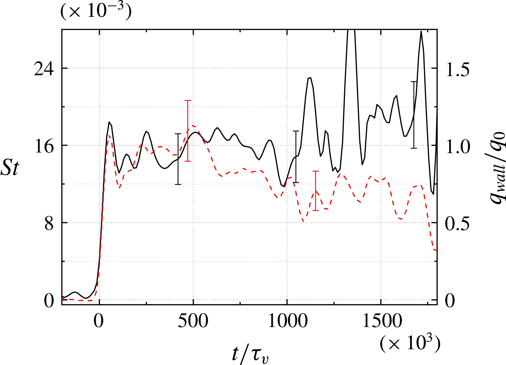
From figures 11 and 19, it is apparent that the peak sustained heat fluxes occur at the upstream base of the cylinder. Noting again the earlier study of Estruch (Reference Estruch2016), which indicated that the peak heating ahead of a blunt obstacle in hypersonic flow scales with the stagnation-point heating value,
 $q_{0}$
(3.2), in figure 23 we plot the time-resolved heat flux at
 $x/r=-1.4$
,
 $y=0$
, both as a Stanton number and normalized by
 $q_{0}$
, for both cylinder heights. This value of
 $x/r$
was the closest point to the cylinder base at which TSP measurements could be reliably extracted. For
 $h/r=10$
,
 $q_{wall}/q_{0}$
remains close to unity throughout the laminar and transitional development. Following the collapse of the interaction zone back towards the cylinder at
 $t/\unicode[STIX]{x1D70F}_{v}\approx 750$
(which coincides with the clear formation of the upstream horseshoe vortex), the mean level increases slightly and the large-scale oscillations noted earlier, produced as incoming turbulent structures, are incident upon the interaction. For
 $h/r=3.7$
, the initial heating during the laminar phase is very similar (
 $q_{wall}/q_{0}\approx 1$
), which might have been expected considering both cylinders are significantly larger than the boundary-layer thickness at these early times (figure 7). Following transition, however, this peak heating reduces gradually to
 $q_{wall}/q_{0}\approx 0.7$
, and although some oscillations are observed, these are significantly reduced in amplitude compared to
 $h/r=10$
(13 % RMS variation about the mean between
 $t/\unicode[STIX]{x1D70F}_{v}=1000$
and 1700, compared to 22 % for
 $h/r=10$
). These laminar and turbulent peak heating levels are very similar to those observed by Estruch (Reference Estruch2016) for short,
 $90^{\circ }$
obstacles in a Mach 8.2 boundary-layer flow (
 $q_{wall}/q_{0}\approx 0.9$
and 0.7, respectively).
Normalized heat flux versus time at
 $x/r=-1.4$
for
 $h/r=10$
(——), and 3.7 (– –), both with Condition A.

3.3.3 Effect of varying the unit Reynolds number
We now examine the combined effects of varying the unit Reynolds number and the cylinder height. Experimentally derived
 $x$
–
 $t$
diagrams of the Stanton number for all three conditions with
 $h/r=3.7$
are presented in figure 24. As the unit Reynolds number is decreased, the heat flux immediately upstream of the cylinder becomes higher over a larger streamwise extent; comparing to the
 $h/r=10$
diagrams in figure 14, the heating in this region also exhibits reduced fluctuation levels, particularly during the period in which the incoming boundary layer is laminar. In the Condition C,
 $h/r=3.7$
experiment, the laminar flow period was unusually long (the
 $t/\unicode[STIX]{x1D70F}_{v}$
value at transition was approximately
 $550\times 10^{3}$
for Condition C and approximately
 $360\times 10^{3}$
for Conditions A and B). This appears to be the only case examined in which the upstream interaction zone had finished growing before the incoming boundary layer became turbulent. Downstream of the cylinder, we note that the Stanton numbers are generally higher for the lower unit Reynolds numbers. Furthermore, especially during the laminar period, the
 $h/r=3.7$
heating levels exceed those for
 $h/r=10$
.
Experimentally derived
 $x$
–
 $t$
diagrams of the Stanton number along the centreline with
 $h/r=3.7$
for (a–c) Condition A to C.

In figure 25, we compare the time-resolved Stanton number curves for the three different flow conditions at two locations using the viscous normalization. At the upstream location (
 $x/r=-2.3$
, figure 25
a), we note immediately that the three curves show more variation between them than the corresponding
 $h/r=10$
profiles. Part of this discrepancy is a result of the somewhat delayed transition in the Condition-C experiment, as noted earlier. Nevertheless, additional variation may be expected since, in the case of a small protuberance, the ratio
 $h/\unicode[STIX]{x1D6FF}$
will become an additional parameter in the problem. At the downstream location (
 $x/r=3.3$
, figure 25
b), we again see a relatively poor collapse of the curves with the
 $t/\unicode[STIX]{x1D70F}_{v}$
scaling, which is probably a result of both the two effects (variable transition and influence of
 $h/\unicode[STIX]{x1D6FF}$
) just described for the upstream profiles and the increased significance of inviscid time scales in the wake region, as discussed in relation to the corresponding
 $h/r=10$
curves.
Time-resolved Stanton number curves for
 $h/r=3.7$
at the following locations along the centreline: (a)
 $x/r=-2.3$
; (b)
 $x/r=3.3$
. In each plot, the different curves correspond to: ——, Condition A; – –, Condition B; – ⋅ – ⋅ –, Condition C.

This poor agreement downstream of the cylinder is also seen in figure 26, which compares instantaneous Stanton number profiles along the centreline for the three conditions at three values of
 $t/\unicode[STIX]{x1D70F}_{v}$
. At none of these times do the downstream parts of the curves show a good collapse. The upstream agreement is somewhat better, though again not as satisfactory as for the larger cylinder. At
 $t/\unicode[STIX]{x1D70F}_{v}=746\times 10^{3}$
, in both the Condition B and C curves we observe the characteristic hump upstream of the cylinder that suggests the presence of secondary horseshoe vortices.
Instantaneous Stanton number profiles along the centreline for
 $h/r=3.7$
at times: (a)
 $t/\unicode[STIX]{x1D70F}_{v}=105\times 10^{3}$
; (b)
 $t/\unicode[STIX]{x1D70F}_{v}=262\times 10^{3}$
; (c)
 $t/\unicode[STIX]{x1D70F}_{v}=746\times 10^{3}$
. In each plot, the individual lines correspond to: ——, Condition A; – –, Condition B; – ⋅ – ⋅ –, Condition C. The symbols correspond to instantaneous thermocouple measurements at the relevant times: ▵, Condition A; ▫, Condition B; ○, Condition C.

4 Conclusions
We have investigated the unsteady flow phenomena produced by the interaction of a shock-induced, Mach 1.2 boundary-layer flow with a wall-mounted circular cylinder. To the authors’ knowledge, this is the first extensive study of a temporally developing supersonic boundary-layer flow over an obstacle in the literature. Because of the complex flow fields and intrinsically short time scales of this problem, experimental techniques both having a very fast response time and capable of global measurements are highly desirable. We have employed a fast response TSP to make measurements of the time-resolved surface heat flux at the wall and, through combination with high-speed schlieren visualizations, drawn links with the inviscid external flow features.
For the large protuberance (
 $h/r=10$
), following the passage of the incident shock, a region of enhanced heating spread ahead of the cylinder as the bow shock propagated upstream. The maximum instantaneous heating level recorded during this development was more than 50 % higher than the estimated stagnation-point heating on the cylinder. Near the foot of the cylinder, the peak heating level remained approximately equal to this stagnation-point value. The SWBLI produced by the bow shock led to transition to turbulence of the laminar boundary layer as it passed through the interaction, producing transient streaks in the surface heat flux. Following natural transition of the incoming boundary layer, the region of enhanced heating withdrew towards the cylinder, though the shock location remained essentially unchanged. Large fluctuations in the heating levels, especially near the foot of the cylinder, were observed to be caused by incoming disturbances in the turbulent boundary layer, and a distinctive bow-shaped feature upstream of the cylinder suggested the presence of secondary horseshoe vortices. The upstream flow development at different unit Reynolds numbers collapsed fairly well with a viscous/Stanton number scaling, following an initial period (upstream shock propagation) during which inviscid scaling was more appropriate.
Downstream of the large protuberance, a fan-shaped region of increased heating formed that appeared to be associated with the recompression shock behind the cylinder. Immediately following transition of the incoming boundary layer, the apparent spatial origin of this fan-shaped region – which we have referred to here as the apex – moved upstream to immediately behind the cylinder (1–2 radii downstream of the trailing edge); the peak heating at this apex region also increased significantly during this upstream motion. The flow development downstream of the cylinder for different unit Reynolds numbers did not collapse as successfully with the viscous scaling as the upstream region, suggesting an increased importance of the external, inviscid flow phenomena in this region.
Measurements with a small (
 $h/r=3.7$
) protuberance revealed many of the same qualitative features as in the
 $h/r=10$
case, though with a reduced spatial footprint. In general, the upstream heating levels were lower for the smaller protuberance (though the maximum heating during the laminar flow period was similar), whereas the downstream heating levels were higher, particularly when the incoming boundary layer was laminar. The peak heat loading at the apex region, on the other hand, was reduced compared to
 $h/r=10$
. Comparing between the various Reynolds numbers, neither the viscous nor the inviscid scaling was found to collapse the data satisfactorily, perhaps pointing to the increased importance of the parameter
 $h/\unicode[STIX]{x1D6FF}$
for small protuberances.
The present measurements have demonstrated conclusively the usefulness of fast-response TSP techniques in investigating unsteady flow configurations on very short time scales. An obvious extension of the present work would be an investigation of the same cylindrical geometry but employing different incident shock Mach numbers; Sedney (Reference Sedney1973) and Lakshmanan & Tiwari (Reference Lakshmanan and Tiwari1994), for example, note that the flow field in such a configuration can change qualitatively with varying
 $M$
. As the post-shock Mach number for a simple shock tube is limited to a maximum of 1.89 for air, it would be quite feasible to fully characterize the cylinder interaction problem within the supersonic post-shock regime.
Supplementary movies
Supplementary movies are available at https://doi.org/10.1017/jfm.2018.433.