


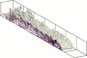


1. Introduction
Unsteady gravity currents, or finite volume gravity currents, are a common type of intermittent buoyancy-driven flow. They form when a finite volume of dense fluid suddenly discharges into a lighter quiescent environment and propagates as an avalanche-like dense wave. The density difference can be caused by either temperature gradients, compositional concentration gradients or an inhomogeneous distribution of suspended sediment in the case of turbidity currents. Notable types of unsteady gravity currents are underwater reservoir discharges, river and estuary outflows and subaqueous landslides (Meiburg & Kneller Reference Meiburg and Kneller2010).
Unsteady gravity currents have been the focus of much research, and are commonly reproduced in a laboratory by the sudden release of a fixed volume of fluid into a channel using the lock-exchange technique (Rottman & Simpson Reference Rottman and Simpson1983; Härtel, Meiburg & Necker Reference Härtel, Meiburg and Necker2000; Cantero et al. Reference Cantero, Balachandar, Garcia and Bock2008; Fragoso, Patterson & Wettlaufer Reference Fragoso, Patterson and Wettlaufer2013; Nogueira et al. Reference Nogueira, Adduce, Alves and Franca2014; Inghilesi et al. Reference Inghilesi, Adduce, Lombardi, Roman and Armenio2018; Kyrousi et al. Reference Kyrousi, Leonardi, Roman, Armenio, Zanello, Zordan, Juez and Falcomer2018; Lombardi, Adduce & La Rocca Reference Lombardi, Adduce and La Rocca2018; Ottolenghi et al. Reference Ottolenghi, Prestininzi, Montessori, Adduce and La Rocca2018; Pelmard, Norris & Friedrich Reference Pelmard, Norris and Friedrich2018; Pérez-Díaz et al. Reference Pérez-Díaz, Castanedo, Palomar, Henno and Wood2018a,Reference Pérez-Díaz, Palomar, Castanedo and Alvarezb; Wilson, Friedrich & Stevens Reference Wilson, Friedrich and Stevens2018b; Zhao et al. Reference Zhao, He, Lv, Lin, Hu and Pähtz2018). The structure of gravity currents can be divided into three parts: an active dense frontal head, followed by a long body akin to a stratified shear layer and a decayed tail (Middleton Reference Middleton1966; Komar Reference Komar1972; Kneller, Bennett & McCaffrey Reference Kneller, Bennett and McCaffrey1999) (see figure 1). The three phases of the current's propagation – namely the initial slumping phase, the inertial phase and the buoyant–viscous phase – are well understood and dimensional analysis and shallow-water models have permitted the derivation of self-similar laws for the front velocity of the current (Benjamin Reference Benjamin1968; Bonnecaze, Huppert & Lister Reference Bonnecaze, Huppert and Lister1993; Shin, Dalziel & Linden Reference Shin, Dalziel and Linden2004), which have been validated against experimental and numerical datasets (Keulegan Reference Keulegan1957; Middleton Reference Middleton1966; Rottman & Simpson Reference Rottman and Simpson1983; Marino, Thomas & Linden Reference Marino, Thomas and Linden2005; Cantero et al. Reference Cantero, Lee, Balachandar and Garcia2007).
Schematic representation of the lock-exchange geometry (based on Wilson et al. Reference Wilson, Friedrich and Stevens2017) and the induced gravity current. Dimensions:  $H = 0.3\ \textrm {m}$,
 $L_{x,l} = 0.58\ \textrm {m}$,
 $L_{x,c} = 5.58\ \textrm {m}$ and
 $L_z = 0.4\ \textrm {m}$, with 2 % inclination.

The interfacial dynamics of gravity currents is often modelled as stratified shear layers. Shear not only triggers the growth of three-dimensional turbulence at high Reynolds numbers, but also excites Kelvin–Helmholtz instabilities in the presence of flow stratification. The amplification of the Kelvin–Helmholtz instabilities leads to the roll up of the current's interface into two-dimensional Kelvin–Helmholtz billows which subsequently entrain ambient fluid into the current and drives the growth of an interfacial mixing layer (Britter Reference Britter1974; Hacker, Linden & Dalziel Reference Hacker, Linden and Dalziel1996; Hallworth et al. Reference Hallworth, Huppert, Phillips and Sparks1996; Härtel et al. Reference Härtel, Meiburg and Necker2000; Ottolenghi et al. Reference Ottolenghi, Adduce, Inghilesi, Armenio and Roman2016a,Reference Ottolenghi, Adduce, Inghilesi, Roman and Armeniob; Ottolenghi, Cenedese & Adduce Reference Ottolenghi, Cenedese and Adduce2017b).
Modelling approaches have aimed to specify the effect of shear induced mixing on the evolution of the averaged flow quantities. One such quantity is the bulk Richardson number, defined as the ratio of the density to the velocity difference at the sides of the mixing layer (Ellison & Turner Reference Ellison and Turner1959; Turner Reference Turner1986; Cenedese & Adduce Reference Cenedese and Adduce2010). The evaluation of the turbulence kinetic energy (TKE) budget allows direct estimation of turbulence suppression in the presence of stable stratification using the flux Richardson number  $Ri_f$, which quantifies the ratio of buoyant destruction to shear production of turbulence (Ellison Reference Ellison1957; Britter Reference Britter1974; Osborn Reference Osborn1980). However, in most experimental and in situ flow studies, the second-order statistics necessary for the calculation of
 $Ri_f$ are not available and several attempts have been made to parameterise
 $Ri_f$ in terms of the gradient Richardson number
 $Ri_g$ across the interface of the mixing layer (Townsend Reference Townsend1958; Britter Reference Britter1974; Pacanowski & Philander Reference Pacanowski and Philander1981; Mellor & Yamada Reference Mellor and Yamada1982; Strang & Fernando Reference Strang and Fernando2001; Odier, Chen & Ecke Reference Odier, Chen and Ecke2014). The validity of these models was notably shown to hold for
 $Ri_g$ smaller than the value
 $Ri_{g,c} = 0.25$, identified theoretically as the critical threshold value below which the mixing layer starts being unstable to Kelvin–Helmholtz instabilities (Thorpe Reference Thorpe1968; Townsend Reference Townsend1980).
Most geophysical models assume the current to be steady and neglect the influence of the head on the current dynamics. Whilst such assumptions are acceptable for field-scale currents, such as oceanic overflows and atmospheric cold air waves that exhibit a large length to height aspect ratio, their application to unsteady gravity currents is questionable. Recent experimental observations (Hacker et al. Reference Hacker, Linden and Dalziel1996; Kneller et al. Reference Kneller, Bennett and McCaffrey1999; Thomas, Dalziel & Marino Reference Thomas, Dalziel and Marino2003; Sher & Woods Reference Sher and Woods2015) highlighted the central role of the flow dynamics in the head on the development of the mixing layer. In particular, the TKE budget in the mixing layer is expected to be significantly affected by the dilution of the head and the subsequent loss of the buoyancy force driving the propagation of the current. laser Doppler velocimetry (LDV) measurements of the flow in the head of a moderately turbulent lock-exchange gravity current by Kneller et al. (Reference Kneller, Bennett and McCaffrey1999) reported singular patchy regions of negative vertical momentum fluxes in the front region, which contrasts with the positive fluxes characteristic of stratified flows observed in the body. More recent numerical studies show similar results for the density turbulence flux, which acts to confine the dense fluid inside the current at the leading edge and leads to the intensification of turbulence by buoyancy (Ottolenghi et al. Reference Ottolenghi, Adduce, Inghilesi, Armenio and Roman2016a; Bhaganagar Reference Bhaganagar2017). However, a thorough discussion of the dynamics of the flow at the front of the current is still lacking to the authors’ knowledge.
1.1. Objectives
The present work is motivated by a lack of information on the spatial evolution of the mixing layer of unsteady gravity currents, notably along the head and its direct wake. Three-dimensional large eddy simulations (LES) of a fully turbulent lock-exchange gravity current were performed. LES simulations have been shown to accurately predict the behaviour of high Reynolds lock-exchange gravity currents at reasonable computational costs (Bonometti & Balachandar Reference Bonometti and Balachandar2008; Ooi, Constantinescu & Weber Reference Ooi, Constantinescu and Weber2009; Özgökmen, Iliescu & Fischer Reference Özgökmen, Iliescu and Fischer2009; Tokyay, Constantinescu & Meiburg Reference Tokyay, Constantinescu and Meiburg2012, Reference Tokyay, Constantinescu and Meiburg2014; Meiburg, Radhakrishnan & Nasr-Azadani Reference Meiburg, Radhakrishnan and Nasr-Azadani2015; Ottolenghi et al. Reference Ottolenghi, Adduce, Inghilesi, Roman and Armenio2016b, Reference Ottolenghi, Adduce, Roman and Armenio2017a; Kyrousi et al. Reference Kyrousi, Leonardi, Roman, Armenio, Zanello, Zordan, Juez and Falcomer2018; Pelmard et al. Reference Pelmard, Norris and Friedrich2018). A two-dimensional description of the turbulence statistics is generated by ensemble averaging 200 separate simulations and spanwise averaging (span averaging) of the domain. The ensemble-averaged statistics are presented for two time steps chosen to represent the slumping and inertial phases of the current's propagation. The numerical model and the averaging approaches used to compute the momentum and transport fluxes are introduced in § 2. In § 3, the current's propagation and the growth of the mixing layer are characterised. Section 4 focuses on identifying the changes in the turbulence dynamics of the mixing layer at the head to body transition. Finally, the TKE budget is evaluated in § 5 and the flow dependency on the flux and gradient Richardson numbers is assessed.
2. Numerical model and simulations
2.1. Analytical formulation
The physical configuration studied is shown in figure 1 and inspired by Wilson, Friedrich & Stevens (Reference Wilson, Friedrich and Stevens2017). In their experiments, the lock on the left was initially filled with a fluid of density  $\rho _1$ and the channel on the right was filled with an ambient fluid of lower density
 $\rho _0$. The current was triggered by suddenly releasing the dense fluid into the channel at
 $t = 0$.
The fluid's motion was studied by solving the three-dimensional LES form of the incompressible Navier–Stokes equations, together with a transport equation for the local density variations. Since the density varies by less than 8 %, closure between the transport and density equations is assured by applying the Boussinesq approximation (Meiburg & Kneller Reference Meiburg and Kneller2010). The equations were rendered dimensionless using the half-lock height  $H/2$, the buoyancy velocity
 $u_b = \sqrt {g'(H/2)}$ with the reduced gravity
 $g' = g(\rho _1 - \rho _0)/\rho _0$ and
 $t_0 = (H/2)/u_b$ as the length, velocity and time scales respectively. The dimensionless density was defined as
 $m = (\rho - \rho _0)/(\rho _1 - \rho _0)$ and varies between 0 and 1. The physical quantities are denoted with a tilde (i.e.
 $\tilde {\phi }$) and their dimensionless counterparts without (i.e.
 $\phi$). Defining the overbar
 $\overline {\phi }$ as the LES filtering operator, the LES set of equations takes the form (Smagorinsky Reference Smagorinsky1963)
 \begin{gather} \frac{\partial \overline{u}_i}{\partial x_i} = 0, \end{gather}
 \begin{gather}\frac{\partial \overline{u}_i}{\partial t} + \frac{\partial \overline{u}_i \overline{u}_j}{\partial x_j} ={-}\frac{\partial \overline{p}}{\partial x_i} + \frac{\partial }{\partial x_j}\left[ \frac{1}{Re} \frac{\partial \overline{u}_i}{\partial x_j} \right] - \frac{\partial \tau_{ij}}{\partial {x_j}} + \overline{m} e_i^{g}, \end{gather}
 \begin{gather}\frac{\partial \overline{m}}{\partial t} + \frac{\partial \overline{u}_i \overline{m}}{\partial x_i} = \frac{\partial }{\partial x_i}\left[ \frac{1}{Sc \,Re} \frac{\partial \overline{m}}{\partial x_i} \right] - \frac{\partial \tau_i^{m}}{\partial {x_i}}, \end{gather}
with  $e_i^{g}$ the unit gravity vector. The dimensionless quantities embodying the physical properties of the flow are the Reynolds number
 $Re = u_b (H/2) / \nu$ and the Schmidt number
 $Sc = \nu /\varGamma$, where
 $\nu$ is the kinematic viscosity and
 $\varGamma$ is the density diffusivity. The momentum and density residual stresses
 $\tau _{ij}$ and
 $\tau _i^{m}$ correspond to the effects of the unresolved turbulent structures smaller than the filter width. The momentum residual stresses are modelled using the standard Smagorinsky model (Smagorinsky Reference Smagorinsky1963);
 $\tau _{ij}$ is expressed as a function of the corresponding resolved strain tensor
 $\overline {\boldsymbol{\mathsf{S}}}_{ij}$ and a numerical subgrid-scale (SGS) viscosity
 $\nu _{SGS}$.
 \begin{gather} \tau_{ij} ={-}2 \nu_{SGS} \overline{\boldsymbol{\mathsf{S}}}_{ij}, \end{gather}
 \begin{gather}\nu_{SGS} = (C_s \varDelta)^{2} \sqrt{\overline{\boldsymbol{\mathsf{S}}}_{ij} \overline{\boldsymbol{\mathsf{S}}}_{ij}}, \end{gather}
 \begin{gather}\overline{\boldsymbol{\mathsf{S}}}_{ij} = \frac{1}{2} \left(\frac{\partial \overline{u}_i}{\partial x_j} + \frac{\partial \overline{u}_j}{\partial x_i} \right). \end{gather}
The Smagorinsky coefficient usually varies between 0.1 and 0.2 (Pope Reference Pope2000) and was set to  $C_s = 0.18$ (Pelmard et al. Reference Pelmard, Norris and Friedrich2018). The filter width is locally defined from the cell size volume as
 $\varDelta = V^{1/3}$. Similarly, the density residual stresses
 $\tau _i^{m}$ were modelled as diffusive fluxes by introducing a SGS diffusivity
 $\varGamma _{SGS}$ calculated using a fixed SGS Schmidt number
 $Sc_{SGS} = \nu _{SGS}/\varGamma _{SGS} = 0.7$ (Pelmard et al. Reference Pelmard, Norris and Friedrich2018). A no-slip boundary condition was imposed at the bottom wall, whereas symmetry conditions were chosen for the side walls and slip walls at the backward and forward walls.
2.2. Numerical model
The simulations were carried out using the structured non-staggered Cartesian finite volume SnS code (Norris Reference Norris2000). The filtered equations were solved using a fractional-step method, with the advection terms discretised in time using an Adams–Bashforth scheme and a Crank–Nicholson scheme for the diffusion terms. Second-order central differencing was used for the spatial discretisation of the advection and diffusion terms. The time step was varied to maintain the value of the Courant–Lewy–Friedrich number ( $CFL = u {\rm \Delta} t / {\rm \Delta} x$) in the range 0.15–0.25.
The fluid filling the channel was initially at rest and a random velocity perturbation  $-0.45 < u_i < 0.45$ was imposed inside the lock to accelerate the development of turbulence. This also mimicked the stirring of the dense fluid to homogenise the density before opening the gate done by Wilson et al. (Reference Wilson, Friedrich and Stevens2017). The initial velocity field was corrected to satisfy the divergence free condition imposed by the continuity equation (2.1). In line with the experiments of Wilson et al. (Reference Wilson, Friedrich and Stevens2017), the Reynolds number was set to
 $Re = 60\ 000$. This Reynolds number is large enough for the behaviour of the fluid to be globally insensitive to the Schmidt number (Bonometti & Balachandar Reference Bonometti and Balachandar2008) when
 $Sc > 1$ and its value is here set to
 $Sc = 1$ (Necker et al. Reference Necker, Härtel, Kleiser and Meiburg2002, Reference Necker, Härtel, Kleiser and Meiburg2005; Cantero et al. Reference Cantero, Balachandar, Garcia and Bock2008; Ooi et al. Reference Ooi, Constantinescu and Weber2009; Özgökmen et al. Reference Özgökmen, Iliescu and Fischer2009; Nasr-Azadani & Meiburg Reference Nasr-Azadani and Meiburg2011).
2.3. Statistical treatment of the current
The statistical treatment of turbulence is based on the Reynolds decomposition of the physical quantities, which aims to dissociate the averaged behaviour of the flow from the local variations due to turbulent perturbations. Introducing the Reynolds ensemble-averaging operator  $\langle \rangle$, each physical quantity
 $\phi$ is decomposed as
 $\phi = \varPhi + \phi '$, in which the capital letter
 $\varPhi = \langle \phi \rangle$ represent the averaged value of
 $\phi$ and
 $\phi '$ is the turbulent perturbation about this average. The averaged set of equations thus reads
 \begin{gather} \frac{\partial U_i}{\partial x_i} = 0, \end{gather}
 \begin{gather}\frac{\partial U_i}{\partial t} + \frac{\partial U_i U_j}{\partial x_j} ={-}\frac{\partial P}{\partial x_i} + \frac{\partial }{\partial x_j}\left[ \frac{1}{Re} \frac{\partial U_i}{\partial x_j} \right] - \frac{\partial \boldsymbol{\mathsf{S}}_{ij}}{\partial {x_j}} - \frac{\partial \langle {u'_i u'_j} \rangle}{\partial x_j} + M e_i^{g}, \end{gather}
 \begin{gather}\frac{\partial M}{\partial t} + \frac{\partial U_i M}{\partial x_i} = \frac{\partial }{\partial x_i}\left[ \frac{1}{Sc \,Re} \frac{\partial M}{\partial x_i} \right] - \frac{\partial T_i^{m}}{\partial {x_i}} - \frac{\partial \langle {u'_i m'} \rangle}{\partial x_j}, \end{gather}
with  $\boldsymbol{\mathsf{S}}_{ij} = \langle \tau _{ij} \rangle$ and
 $T_i^{m} = \langle \tau _i^{m} \rangle$. To simplify the presentation, the overbars are dropped in the averaged equations, however, the variables still refer to the filtered physical quantities.
Lock-exchange gravity currents are inhomogeneous in space and transient in nature. Therefore, the standard methods of calculating turbulent statistics by averaging in space or time are inappropriate. Making use of the statistical two-dimensional nature of the flow, the statistics are first computed from averaging over the  $N_z$ spanwise cells of the domain (span averaging). Considering the limited width of the domain, span averaging only provides a rough statistical description of the flow and a significantly higher number of cells is required to achieve convergence of the Reynolds stresses. For comparison, Chang & Lee (Reference Chang and Lee2017) required more than 10 000 individual frames recorded using particle image velocimetry (PIV) measurements of a planar turbulent shear layer to reach satisfactory statistics.
Consequently, a dataset was generated by ensemble averaging 200 separate simulation results, together with span averaging of the flow. Data were computed at two time steps,  $t = 29.1$ and
 $t = 50$ judged representative of the mixing layer's behaviour during the slumping and inertial phases of the current's propagation, respectively. Each simulation was initialised with different random velocity perturbations inside the lock. The simulations present similar evolution during the first instants of the current's propagation. However, they develop sufficiently different turbulence histories to provide a chaotic distribution of the Kelvin–Helmholtz billows over the sample of simulations and allow the complete smoothing of the averaged flow to represent the continuous decay of the Reynolds stresses along the current once the mixing layer is fully formed.
2.4. Grid resolution
Two grid sets M1 and M2, based on the grid sensitivity study of Pelmard et al. (Reference Pelmard, Norris and Friedrich2018), were used. Both meshes have a uniform grid  $N_x\times (N_{y,w} + N_{y,d}) \times N_z$, corresponding to a general mesh spacing
 $\varDelta$, except in the bottom near-wall region. To ensure
 $y^{+} < 5$ at the bottom wall, the first vertical mesh spacing was set to
 $\varDelta y_1 = 0.00133$ for both M1 and M2 and was progressively increased to
 $\varDelta y = \varDelta$ at
 $y = 2/3$ following a logarithmic law over
 $N_{y,w}$ cells to allow for an aspect ratio of below 1.1 between two consecutive cells. The mesh spacing was kept constant over the remaining
 $N_{y,d}$ cells (
 $2/3 < y < 2$).
The characteristics of M1 and M2 are detailed in table 1. The propagation of the current and the time development of the mixing layer was first investigated using the fine grid M1. To reduce the computational costs, the 200 simulations used to compute the ensemble-averaged statistics were carried out on the coarser grid M2. Both meshes were shown to provide similar predictions of the front velocity and bulk characteristics of the current (Pelmard et al. Reference Pelmard, Norris and Friedrich2018). Whilst providing a coarser representation of the inner dynamics of the flow, M2 was shown to offer a good description of the turbulence dynamics within the current while reducing the computational time  $T_{sim}$ by a factor of approximately 7 when compared to M1 (Pelmard et al. Reference Pelmard, Norris and Friedrich2018). The model was also shown to predict a substantial part of the inertial subrange of the turbulence spectra, and thus the velocity cross-correlations are considered qualitatively acceptable for the purpose of the study.
Characteristics of grids M1 and M2.

The validity of the LES approach and the influence of the initial random velocity perturbation on the development of the turbulence are further presented in appendix.
3. Prediction of the current
3.1. Front velocity
During a gravity current's propagation, the mixing layer is expected to adjust in response to the progressive dilution of the initial dense fluid released and the diminution of the buoyancy force. The overall balance of forces acting upon the current is reflected on the variations of the current's front velocity  $u_f$ (Benjamin Reference Benjamin1968; Shin et al. Reference Shin, Dalziel and Linden2004; Cantero et al. Reference Cantero, Lee, Balachandar and Garcia2007). For the present configuration, Pelmard et al. (Reference Pelmard, Norris and Friedrich2018) showed a weak dependence of the front velocity on the grid resolution and good qualitative prediction of
 $u_f$ during the two main regimes of propagation – namely the slumping phase and the inertial phase. The front velocity is here further compared to the analytical estimates proposed by Shin et al. (Reference Shin, Dalziel and Linden2004), and later validated numerically by Cantero et al. (Reference Cantero, Lee, Balachandar and Garcia2007) using three-dimensional direct numerical simulation (DNS). A non-dimensional measure of the front velocity is typically given using the front Froude number
 $Fr_f = \tilde {u}_f / \sqrt {g' H}$. The time evolution of
 $Fr_f$ obtained for grid M1 is presented in figure 2. The front velocity is derived from the front position
 $x_f$ defined as the maximum streamwise position on the density isoline
 $\bar{m} = 0.1$ using central differencing. The subscripts sl and i used hereafter stem for the slumping phase and the inertial phase, respectively. During the slumping phase, the front travels at a constant rate and
 $Fr_{f,sl} \approx 0.46$, in good agreement with the experimental value
 $Fr_{f,sl} = 0.48$ of Keulegan (Reference Keulegan1957) and the numerical results of Cantero et al. (Reference Cantero, Lee, Balachandar and Garcia2007). The deceleration of the current during the inertial phase agrees well with the scaling law
 $Fr_{f,i} \sim 0.98 ( (L_{x,l} H)/H^{2} )^{1/3} (\tilde {t}/\sqrt {H/g'} )^{-1/3}$ (Cantero et al. Reference Cantero, Lee, Balachandar and Garcia2007), giving
 $Fr_{f,i} \sim 1.22 (\tilde {t}/\sqrt {H/g'} )^{-1/3}$. The transition from the slumping phase to the inertial phase occurs shortly after
 $t = 30$. An estimate of the instant when the transition occurs is given by
 $\tilde {t}_{sl,i}/\sqrt {H/g'} = 0.94 ( (L_{x,l} H)/H^{2} ) / Fr_{f,sl}$ (Cantero et al. Reference Cantero, Lee, Balachandar and Garcia2007). The estimate gives
 $\tilde {t}_{sl,i}/\sqrt {H/g'} = 18.7$ corresponding to
 $t_{sl,i} = 26.4$ with the present non-dimensionalisation, which agrees with the simulation prediction.
Evolution of the front Froude number  $Fr_f$ during the current's propagation.

3.2. Current structure and mixing layer
Figure 3 presents the isosurfaces of density  $\bar{m} = 0.1$ and the density field on the symmetry plane
 $z = 2.67$ at four time steps corresponding to: (i) the formation of the current (
 $t = 8.1$), (ii) the fully developed current during the slumping phase (
 $t = 20.5$), (iii) the late stage of the slumping phase (
 $t = 29.1$) and (iv) the inertial phase (
 $t = 50$). The simulations correctly predict the structure of the flow. Upon the gate opening, the dense fluid starts slumping in the channel (figure 3a). The current remains compact, yet the two flow instabilities characteristic of gravity currents – the Kelvin–Helmholtz instability at the upper interface of the current and the lobe and cleft instability at the front – are clearly developed at
 $t = 8.1$. The velocity perturbation imposed inside the lock leads to the rapid development of three-dimensional turbulence immediately after the lock release, as shown by the deformation of the density isosurface in figure 3(a). The growth of turbulence is reflected by the accentuation of the density isosurface deformation at later time steps. As the flow develops, the current takes its characteristic structure of a dense frontal head, followed by a vertically stratified body. This is identified in figure 3(b) and maintained for the rest of the simulation. After a certain time, a thin decayed tail is observed in the rear of the body (figure 3c,d).
Density isosurface  $\bar{m} = 0.1$ shortly after the release of the lock (
 $t = 8.1$) (a), once the current is fully formed during the slumping phase (
 $t = 17.5$) (b), at the late stage of the slumping phase (
 $t = 29.1$) (c) and during the inertial phase (
 $t = 50$) (d). The distribution of density is also plotted on the symmetry plane
 $z = 2.67$.

In response to the current's propagation, ambient fluid is advected backward above the current. The mixing layer forms in response to the shear induced by the velocity difference at the interface of the current. Standard planar mixing layers are shear dominated flows, where the velocity field at the sides of the mixing layer is perpendicular to the density gradient. Therefore, the establishment of the mixing layer can be identified by tracking the alignment of the velocity vectors with the density isolines at the interface of the mixing layer. Figure 4 shows the velocity vectors in a reference frame moving with the front and the density isolines in the head of the current at  $t = 29.1$ with the horizontal coordinate relative to the front position
 $x_f = 19.3$. Two regions are distinguished. Firstly, the velocity field is perpendicular to the density isolines at the front and progressively aligns with them over a distance of approximately
 $\tilde {x}_f - \tilde {x} \approx H$. Secondly, the velocity vectors align with the density isolines for
 $\tilde {x}_f - \tilde {x} > H$. The structure of the mixing layer is considered fully established once the ambient fluid is advected horizontally for
 $\tilde {x}_f - \tilde {x} > 1.5 H$.
Span-averaged velocity vectors in the head of the current superimposed with the density isolines  $\bar{m} = 0.05$, 0.25, 0.5, 0.75 and 0.95 at
 $t = 29.1$. The velocity vectors are presented in a reference frame moving with the front.

3.3. Turbulent mixing layer
The mixing layer is a region where shear, buoyancy and turbulence interact to generate a complex three-dimensional flow. To identify the behaviour of the mixing layer, one needs to define the mixing layer's borders. Strictly speaking, the standard formulation of the mixing layer's borders as the cross-stream position where the streamwise velocity component reaches 95 % of the outer flow is not directly applicable in the context of gravity currents since no outer flow is imposed. Chang & Li (Reference Chang and Li2011) propose an alternative vorticity based formulation of the mixing layer. Dissociating the shear contribution of vorticity – shear-induced vorticity – from the residual contribution added by the intrinsic local rotation of turbulent structures as  $\omega _z = \omega _{SH} + \omega _{res}$, the borders of the mixing layer are identified as the position where the shear-induced vorticity equals 0. In the present case,
 $\bar {\omega }_{res}$ is found to be more than one order of magnitude smaller than
 $\bar {\omega }_{SH}$ in the vicinity of the mixing layer's borders. The vorticity thus reduces to
 $\bar {\omega }_z \approx \bar {\omega }_{SH}$ and the mixing layer is identified by
 $\bar {\omega }_z > 0$. This definition is equivalent to the enstrophy formulation used by Krug et al. (Reference Krug, Holzner, Luthi, Wolf, Kinzelbach and Tsinober2015) to study the turbulent/non-turbulent interface of a continuously supplied wall-bounded upward propagating gravity current. Inside the current,
 $\bar {\omega }_z$ is negative in the near-wall region and positive in the mixing layer, thence the inner, or bottom, border is easily identified as the height
 $y_b$, where
 $\bar {\omega }_z$ changes sign. Above the current,
 $\bar {\omega }_z$ decays to 0 and the outer, or top, border is diffuse. The top border is thus chosen as the height
 $y_t$, where
 $\bar {\omega }_z$ reaches 5 % of the vorticity scale
 $0.05 u_b/(H/2) = 0.12$, reduced to
 $\bar {\omega }_z = 0.1$.
Figure 5 shows the distribution of the span-averaged TKE along the current as well as the isoline  $\bar {\omega }_z = 0.1$ during the formation of the current (
 $t = 8.1$), once the current is fully formed during the slumping phase (
 $t = 14$ and 20.9) shortly before the transition to the inertial phase (
 $t = 29.1$) and during the inertial phase (
 $t = 39.6$, 50 and 64). The plots are presented in a reference frame moving with the front and the origin is set at the current's front. The TKE is mainly confined in the mixing layer. As the current advances, the width of the mixing layer remains approximately constant over the establishment region
 $\tilde {x}_f - \tilde {x} < H$ identified in figure 4 and expands horizontally similar to a wall-bounded jet for
 $\tilde {x}_f - \tilde {x} > H$ (Townsend Reference Townsend1980). In line with the formation of the head/body structure, the turbulent mixing layer is still forming at
 $t = 8.1$ and the Kelvin–Helmholtz billows are identified by the roll up of the mixing layer and local maxima of TKE at the centre of the rolls. As the current advances, the growth of three-dimensional turbulence tends to partially hide the presence of the billows. At
 $t = 20.9$, the turbulent mixing layer is considered established and the TKE displays a characteristic evolution trend along the current: the TKE increases along the head and decays along the body. The structure of the mixing layer at the front adjusts once the current enters the inertial phase, which is here assumed to be a consequence of the dilution of the head during this phase of propagation.
Span-averaged TKE along the current at  $t = 8.1$, 14, 20.9, 29.1, 39.6, 50 and 64. The contour lines correspond to the isoline
 $\bar {\omega }_z = 0.1$ defining the mixing layer's borders. The plots correspond to the grid M1, and the ensemble-averaged data are shown at
 $t = 29.1$ and 50 for comparison.

The ensemble-averaged fields are also plotted at  $t = 29.1$ and 50 for comparison. The ensemble-averaged fields capture well the behaviour of the mixing layer during the slumping and inertial phases. The ensemble-averaging process totally smooths the Kelvin–Helmholtz billows and gives a continuous and diffuse TKE field.
Note that a region of high TKE is observed in the rear of the current, above the tail, which is induced by a persistent stagnant circulation in the vicinity of the lock gate position. Investigating the nature of this circulation is beyond the scope of this study and is not discussed herein.
4. Statistical characterisation of the current structure
4.1. Definition of the head
The position  $x_h$ where the head ends – referred to hereafter as the limit of the head – is conventionally identified where the Kelvin–Helmholtz billows detach from the head. The limit of the head
 $x_h$ is here defined as the streamwise position from the front where ‘the first local meaningful minimum’ of the depth-averaged height of the current
 $h_c$, defined by (4.1), is obtained. The notion of ‘first local meaningful minimum’ is illustrated in figure 6 by the transition from the blue plain lines to the red dashed lines.
 \begin{equation} h_c (x,t) = \frac{1}{H} \int_0^{H} \overline{m} \, \textrm{d} \tilde{y}. \end{equation}
Depth-averaged height of the current  $H_c$ along the current and the derivative
 $\partial H_c / \partial x$. Also shown are five instantaneous profiles of
 $h_c$ (fine lines). Red dashed lines show the head and blue lines show the wake of the head.

The depth-averaged height of the ensemble-averaged current  $H_c = \langle h_c \rangle$ as well as its derivative
 $\partial H_c / \partial x$ are shown in figure 6 for
 $t = 29.1$ and 50 as thick lines. The profiles of
 $h_c$ are also plotted for five runs to demonstrate the variation between runs. The front of the current is found at
 $\tilde {x}_f = 9.66 H$ and
 $16H$ relative to the lock gate at
 $t = 29.1$ and 50, respectively. The limits of the head obtained from the instantaneous fields are represented by the transition between the plain blue lines and dashed red lines. As observed by Härtel et al. (Reference Härtel, Meiburg and Necker2000), the position of the limit of the head is not fixed. Nogueira et al. (Reference Nogueira, Adduce, Alves and Franca2014) analysed experimentally the evolution of the head of lock-exchange currents for
 $Re$ varying from
 $40\,000$ and
 $60\,000$, using the present definition of
 $Re$. They observed a periodic variation of the head's length as a result of cycles of stretching and contraction of the head.
The instantaneous values of  $\tilde {x}_h$ are confined to the region
 $1.475 H < \tilde {x}_f - \tilde {x}_h < 1.725 H$ of length
 $H/4$, represented in figure 6 by vertical dashed lines, and delimited by the maxima of
 $\partial H_c / \partial x$, at both
 $t = 29.1$ and 50. The predictions of
 $x_h$ agree well with the results presented by Härtel et al. (Reference Härtel, Meiburg and Necker2000, figure 14) and the division of the current as presented by Cantero et al. (Reference Cantero, Balachandar, Garcia and Bock2008, figure 6). The limit of the head is taken as the right border of the previously identified region and set to
 $x_h = 1.5H$ hereafter. It is important to note that Härtel et al. (Reference Härtel, Meiburg and Necker2000) have reported the limit of the head farther upstream from the front, in the range
 $2.5 H < \tilde {x}_f - \tilde {x}_h < 4 H$. Indeed, they defined the head as the position at which the current reaches a quasi-constant minimum height, a state that cannot be achieved in this study due to a significantly lower volume of released dense fluid. The maximum height
 $H_{c} = 0.18$ is reached for
 $\tilde {x}_f - \tilde {x}_h \approx H$, which compares well with the maximum height
 $h_{c} \approx 0.2 H$ obtained at
 $\tilde {x}_f - \tilde {x}_h \approx H$ shown in Härtel et al. (Reference Härtel, Meiburg and Necker2000).
4.2. Turbulence anisotropy of the mixing layer
The transition of the head to the body is well represented by the evolution of the mixing layer's turbulence. Cantero et al. (Reference Cantero, Balachandar, Garcia and Bock2008) have provided valuable qualitative knowledge on the nature of the turbulence structures composing the mixing layer of lock-exchange gravity currents. They notably described the breakup of the two-dimensional coherent Kelvin–Helmholtz billows into three-dimensional smaller-scale vortices due to turbulent tilting and bending processes, as well as the evolution of the turbulence isotropy along the head and its direct wake. Hence, this section focuses on quantifying the changes experienced by the flow at the transition from the head to the body. The velocity perturbations  $\langle u_i'u_i' \rangle$ and the dominant Reynolds stress
 $\langle u'v' \rangle$ are shown in figure 7. Both time steps display similar features, thus only the data for
 $t = 29.1$ are presented herein.
Distribution of the Reynolds stresses  $\langle u'u' \rangle$ (a),
 $\langle v'v' \rangle$ (b),
 $\langle w'w' \rangle$ (c) and
 $\langle u'v' \rangle$ (d) at
 $t = 29.1$.

The turbulence is seen to switch from a mainly streamwise oriented turbulence in the head to three-dimensional turbulence in the body, although the streamwise component remains dominant. Indeed, whilst  $\langle u'u' \rangle$ decreases with increasing distance from the front, its counterparts
 $\langle v'v' \rangle$ and
 $\langle w'w' \rangle$ grow until they peak close to the limit of the head. Thereafter, the three components decrease at the same rate. The TKE is distributed with half to
 $\langle u'u' \rangle$ and a quarter to
 $\langle v'v' \rangle$ and
 $\langle w'w' \rangle$, and the Reynolds stresses are proportioned
 $\langle u'u' \rangle \approx 2 \langle v'v' \rangle \approx 2 \langle w'w' \rangle$ in the body. This observation is of interest since image and laser tracking velocimetry methods, such as PIV and LDV, offer a two-dimensional representation of the flow and cannot determine the cross-stream flow motion. Consequently, the cross-stream component of turbulence is typically estimated using empirical and anisotropy theory deductions. For instance, Odier et al. (Reference Odier, Chen and Ecke2014) conducted LDV measurements of continuously released gravity currents propagating up a smooth plate and computed the TKE by assuming
 $\langle w'w' \rangle = \langle v'v' \rangle$, which agrees with the present observation.
The local three-dimensionality of turbulence is directly quantifiable using the Reynolds stress anisotropy invariants theory of Lumley & Newman (Reference Lumley and Newman1977) (see Jovanovic Reference Jovanovic2013, for a detailed review). Introducing the normalised anisotropy tensor  ${\boldsymbol{\mathsf{a}}}_{ij}$ and its two invariants
 $I I$ and
 $I I I$ as
 \begin{gather} \boldsymbol{\mathsf{a}}_{ij} = \frac{\langle u_i'u_j' \rangle}{2k} - \frac{\delta_{ij}n}{3}, \quad k = \frac{1}{2} \langle u_i'u_i' \rangle , \end{gather}
 \begin{gather}I I = \boldsymbol{\mathsf{a}}_{ij} \boldsymbol{\mathsf{a}}_{ji}, \end{gather}
 \begin{gather}I I I = \boldsymbol{\mathsf{a}}_{ij} \boldsymbol{\mathsf{a}}_{jk} \boldsymbol{\mathsf{a}}_{ki}. \end{gather}
Lumley & Newman (Reference Lumley and Newman1977) proposed a simple parameterisation of the states of turbulence using the parameter  $J = 1 - (0.5 I I - I I I)$ varying between 0 and 1. High values of
 $J$ correspond to three-dimensional turbulence, with
 $J = 1$ corresponding to perfect isotropy. Fading of
 $J$ indicates strong anisotropy, with
 $J = 0$ representing the state of 1- or 2-component turbulence, achieved when a plane exists where one or two of the Reynolds stress tensors equal zero. Figure 8(a,c) presents the distribution of
 $J$ in the mixing layer of the current for
 $\tilde {x}_f - \tilde {x} < 7 H$ at = 29.1 and 50. As previously observed, turbulence is strongly anisotropic in the nose due to the dominance of streamwise turbulence. The growth of three-dimensional turbulence leads to an overall increase of
 $J$ with distance from the front. This process is better illustrated in figure 8(b,d), which shows point clouds of
 $J$ against the distance from the front. Clear threshold between the head and its rear are visible. The three-dimensionality of turbulence in the body is represented by values of
 $J$ higher than 0.5, with a peak at 0.8 in the centre of the mixing layer.
Distribution of anisotropy invariants parameter  $J = 1 - (0.5 I I - I I I)$ in the mixing layer and point cloud of
 $J$ along the current at
 $t = 29.1$ (a,b) and
 $t = 50$ (c,d). The grey portion of the point clouds corresponds to the head and the black portion corresponds to the body.

While the present work focuses on the mixing layer, we briefly discuss the near-wall turbulence. Two notable regions worthy of note are found in the head and correlate well with the near-wall turbulence described by Cantero et al. (Reference Cantero, Balachandar, Garcia and Bock2008). Firstly, high turbulence is observed in the nose. The associated local maximum  $k = 0.036$ at
 $t = 29.1$ and
 $k = 0.03$ at
 $t = 50$ are in comparison
 $\sim$2 and 1.7 times smaller than the corresponding maximum TKE in the mixing layer
 $k = 0.069$ at
 $t = 29.1$ and
 $k = 0.051$ at
 $t = 50$ (figure 5). The region of intense turbulence is found for
 $\tilde {x}_f - \tilde {x} < 0.35 H$ which agrees well with the location of the rich array of turbulent structures identified in the current's front by Cantero et al. (Reference Cantero, Balachandar, Garcia and Bock2008, figure 6). The figure plotted by Cantero et al. (Reference Cantero, Balachandar, Garcia and Bock2008) shows the presence of horizontal hairpin vortices in this region, which are here reflected by the maximum near-wall
 $\langle u'u' \rangle \approx 0.051$ and
 $\langle w'w' \rangle \approx 0.023$ of the same order of magnitude while
 $\langle v'v' \rangle \sim 0$. Secondly, a region of low turbulence is observed for
 $\tilde {x}_f - \tilde {x} > 0.35 H$, where the TKE becomes 5 to 8 times smaller than the corresponding TKE maximum across the mixing layer. The quasi-streamwise vortices identified by Cantero et al. (Reference Cantero, Balachandar, Garcia and Bock2008) are represented by
 $\langle u'u' \rangle$ being overall 5 times higher than
 $\langle w'w' \rangle$.
4.3. Reynolds stress  $\langle u'v' \rangle$

The Reynolds stress  $\langle u'v' \rangle$, shown in figure 7(d), presents an area of negative values at the leading edge and is positive in the rear part of the head and the body. To discuss the nature and role of the Reynolds stress on the motion of the current, the theoretical behaviour of a parcel of fluid located at the interface of the current is considered. A positive Reynolds stress, such as in the wake of the head, means the upward transport of streamwise momentum, or the forward transport of vertical momentum. Since the inner part of the current is by definition located backward and/or downward from the interface of the current, the parcel of fluid tends to transfer momentum from the current to the ambient fluid, therefore contributing to the ambient fluid's inertia. The current and the ambient fluid move in opposite directions, therefore, it is acceptable to assume for the velocity gradient across the interface of the current to be negative. In this context, the net increase (decrease) of momentum in the ambient fluid (current) leads to a net reduction of the velocity difference between the two fluids – that is the velocity gradient at the interface, hence reducing the shear in the mixing layer. In contrast, the negative
 $\langle u'v' \rangle$ at the leading edge indicates the backward transport of vertical momentum or the downward transport of streamwise momentum, which leads to a net increase (decrease) of momentum in the current (ambient fluid) and causes the increase of shear at the interface of the current.
4.4. Turbulence scaling in the mixing layer
Figure 9 shows the profiles of streamwise velocity and TKE at different positions from the front at both time steps. The data are presented using the vertical similarity coordinate  $\xi = (y - y_b)/l_{\omega }$ used to study shear flows (Townsend Reference Townsend1980);
 $\xi$ is corrected to align the origin with the bottom border of the mixing layer. The mixing layer's length
 $l_{\omega } = y_t - y_b$ is chosen as the characteristic length scale for the mixing layer (Chang & Li Reference Chang and Li2011; Chang & Lee Reference Chang and Lee2017), with
 $y_b$ and
 $y_t$ the bottom and top borders of the mixing layer introduced in § 3.3. The streamwise velocity is normalised by the velocity difference at the sides of the mixing layer
 ${\rm \Delta} U = U(y_b) - U(y_t)$ – i.e. the maximum velocity inside the current and the constant ambient fluid velocity above the current. The TKE is normalised by its maximum value across the mixing layer
 $k_{max}(x)$.
Vertical profiles of normalised streamwise velocity  $U/{\rm \Delta} U$ and TKE
 $k/k_{max}$ at
 $t = 29.1$ (a,c) and
 $t = 50$ (b,d). The profiles have been extracted in the head (
 $\tilde {x}_f - \tilde {x}_1 = H$), at the limit of the head (
 $\tilde {x}_f - \tilde {x}_2 = 1.475H$ and
 $\tilde {x}_f - \tilde {x}_3 = 1.725H$), in the developing wake (
 $\tilde {x}_f - \tilde {x}_4 = 3.4H$) and in the developed body (
 $\tilde {x}_f - \tilde {x}_5 = 7.15H$)

Typical profiles of shear layers are obtained: the streamwise velocity shows an error function-like distribution linking the top and bottom borders of the mixing layer, and the TKE presents a Gaussian-like distribution peaking at the mixing layer's centre, where shearing is at a maximum (Townsend Reference Townsend1980; Vreman, Geurts & Kuerten Reference Vreman, Geurts and Kuerten1997; Balaras, Piomelli & Wallace Reference Balaras, Piomelli and Wallace2001; Yang et al. Reference Yang, Zhang, Chan and Lin2004; Krug et al. Reference Krug, Holzner, Luthi, Wolf, Kinzelbach and Tsinober2013). In particular, the profiles obtained for  $\tilde {x_f} - \tilde {x} > 3.4 H$ compare well with experimental and numerical data reported in the body of lock-exchange currents (Garcia Reference Garcia1994; Gray, Alexander & Leeder Reference Gray, Alexander and Leeder2006; Cantero, Balachandar & Parker Reference Cantero, Balachandar and Parker2009; Eggenhuisen & McCaffrey Reference Eggenhuisen and McCaffrey2012) and unconfined currents (Pérez-Díaz et al. Reference Pérez-Díaz, Palomar, Castanedo and Alvarez2018b; Wilson, Friedrich & Stevens Reference Wilson, Friedrich and Stevens2018a). The velocity gradient remains constant across the mixing layer, except inside the head where it grows towards the centre of the mixing region.
The good superimposition of the normalised velocity and TKE profiles suggests the potential existence of a self-similar regime describing the evolution of the mixing layer in the wake of the head. Note that unlike  $t = 50$, the profile of TKE in the head (
 $\tilde {x}_f - \tilde {x}_1 = H$) at
 $t = 29.1$ slightly deviates from the other positions. This difference is attributed to skewness on the calculation of
 $\xi$ inherited from the increasing sensitivity of
 $l_{\omega }$ to the ratio of the cell size to the thickness of the mixing layer
 $\varDelta /l_{\omega }$ when the mixing layer shrinks. To qualify the existence of a self-similar regime in the mixing layer, the normalising quantities
 ${\rm \Delta} U$ and
 $k_{max}$ are shown in figure 10. The head is characterised by the increase of
 ${\rm \Delta} U$ and
 $k_{max}$. The limit of the head is identified by the sudden change in the trend of
 ${\rm \Delta} U$ and
 $k_{max}$. In a strict sense, no self-similar regime could be identified, since no unique velocity scale was found to describe both the decrease of
 ${\rm \Delta} U$ and
 $k_{max}$ at the same time. However, each quantity follows individual scaling laws, therefore indicating specific similarity of
 $U$ and
 $k$ in the body.
Evolution of the velocity difference at the sides of the mixing layer  ${\rm \Delta} U$ (a) and the maximum TKE over the depth of the mixing layer
 $k_{max}(x)$ (b) along the current.

While  ${\rm \Delta} U$ appears to decrease linearly along the length of the body at both time steps (figure 10a), the switch of decaying trend of the TKE from the apparent exponential scaling
 $\exp [-3.7 (\tilde {x}_f - \tilde {x})/L_c]$ at
 $t = 29.1$ to a power law scaling with
 $( x/x_f )^{-1.1}$ at
 $t = 50$ in the wake of the head suggests the existence of distinct turbulence regimes in the body of the current at the two time steps. The development of different turbulence regimes is likely to be the result of changes in the overall force balance acting upon the current occurring at the transition from the slumping phase to the inertial phase as the dense head starts being diluted. Analytical solutions for the evolution of turbulence in stratified shear flows have been derived for instance by Rohr et al. (Reference Rohr, Itsweire, Helland and Van Atta1988), following the initial solution proposed by Tavoularis (Reference Tavoularis1985) for non-stratified flows. In the present case, such derivations are hindered by the non-satisfaction of several necessary conditions – among others stationary flow conditions, constant eddy viscosity and eddy diffusivity across the mixing layer and constant averaged streamwise velocity – which allow the simplification and analytical resolution of the governing equations. Note that the fitted linear trend of
 ${\rm \Delta} U$ at
 $t = 29.1$ ends where the body collapses into the tail at approximately
 $\tilde {x}_f - \tilde {x} \approx 8H$, and is unlikely to have been influenced by the backward wall circulation identified in § 3.3 (figure 5).
At both time steps, the decay of  $k_{max}$ abruptly stops and plateaus over approximately
 $3H$ (figure 10b). The plateau
 $k_{max} \approx 0.019$ is approximately 3.5 times lower than its maximum at the limit of the head at
 $t = 29.1$, whereas its value
 $k_{max} \approx 0.0055$ at
 $t = 50$ is approximately 9 times lower than the corresponding maximum at the limit of the head. At this stage, no conclusions can be made concerning the nature and evolution of the plateau on the basis of the two time steps studied. However, it illustrates the existence of a regime of horizontally homogeneous turbulence inside the body which would eventually allow for the computation of meaningful statistics using streamwise and spanwise averaging over part or all the length of the plateau. Such statistics would prove valuable for the quantitative validation of LES and DNS simulations of unsteady gravity currents against experimental datasets. The influence of the backward circulation on the existence of the plateau needs, however, to be assessed.
5. Stratified turbulence balance
5.1. TKE budget
The change in the trend of the decay of TKE in the body between  $t = 29.1$ and
 $t = 50$ observed in figure 10(b) suggests the rearrangement of the TKE production/dissipation balance. This section presents and discusses the evolution of the TKE budget along the current. The TKE budget (5.1) is derived from the combination of the instantaneous and averaged flow equations (2.2) and (2.8) as
 $\langle u_i'$ (2.2)–(2.8)
 $\rangle$.
 \begin{equation} \frac{\mathrm{D} k}{\mathrm{D} t} = P + B - \varepsilon + T + D. \end{equation}
The term  ${\mathrm {D} k}/{\mathrm {D} t} = {\partial k}/{\partial t } + U_i {\partial k}/{\partial x_i}$ is the material/Lagrangian derivative describing the rate of variation of TKE held by a parcel of fluid advected by the averaged flow. The three first terms on the right-hand side of (5.1) correspond to the production and destruction of turbulence;
 $P = \langle u_i' u_j' \rangle {\partial U_i}/{\partial x_j}$ is the production of turbulence by shear – i.e. the conversion of energy from the averaged flow to turbulent momentum;
 $B = \langle u_i' m' \rangle e_i^{g}$ is the buoyancy flux responsible for the production/destruction of turbulence (positive/negative) due to buoyant mixing in stratified flows. The dissipation rate of turbulence
 $\varepsilon = ({1}/{Re}) \langle {({\partial u_i'}/{\partial x_j}) ({\partial u_i'}/{\partial x_j})} \rangle - \langle {u_i' {\partial \tau _{ij}'}/{\partial x_j}} \rangle$ comprises the combined effect of the molecular dissipation and SGS diffusion. The last two terms of (5.1) stem from the passive redistribution of TKE in the domain and have no impact on the total energy budget integrated over the simulation domain. Thereby,
 $T = -({1}/{2}) {\partial \langle u_i' u_i' u_j' \rangle }/{\partial x_j}$ is the transport of turbulence by the turbulent perturbations, also interpreted as a turbulent diffusive flux, and
 $D = {\partial }[ -\langle u_j'p' \rangle + (1/Re) {\partial k}/{\partial x_j} ] /{\partial x_j}$ is a cumulative diffusive flux, which includes the pressure and viscous diffusion of turbulence.
To analyse the production/destruction balance and the energy exchanges along the current, (5.1) is averaged over the depth of the domain. Depth averaging is denoted by the operator  $\langle \rangle _d$ and the depth-averaged quantities
 $\langle P \rangle _d$,
 $\langle B \rangle _d$,
 $\langle - \varepsilon \rangle _d$,
 $\langle T \rangle _d$ and
 $\langle D \rangle _d$ are shown in figure 11(a,b) at
 $t = 29.1$ and 50. The different terms of the energy budget (figure 11a,b) present similar evolution trend at both time steps. The turbulent diffusion flux
 $\langle T \rangle _d$ and diffusive flux
 $\langle D \rangle _d$ are negligible as compared to the three other terms and can be neglected in (5.1). The TKE budget reduces then to the balance between the production and destruction terms of TKE
 \begin{equation} \frac{\mathrm{D} \langle k \rangle_d}{\mathrm{D} t} \approx \langle P \rangle_d + \langle B \rangle_d - \langle \varepsilon \rangle_d. \end{equation}
Depth-averaged shear production of turbulence  $\langle P \rangle _d$, buoyant contribution to turbulence
 $\langle B \rangle _d$, dissipation
 $- \langle \epsilon \rangle _d$, turbulent transport
 $\langle T \rangle _d$ and combined pressure and viscous diffusion of turbulence
 $\langle D \rangle _d$ along the current at
 $t = 29.1$ (a) and 50 (b). The Lagrangian derivative of TKE
 $\mathrm {D} \langle k \rangle _d/\mathrm {D}t$ and
 $\langle P \rangle _d + \langle B \rangle _d - \langle \varepsilon \rangle _d$ are shown in (c).

The value of  $\mathrm {D} \langle k \rangle _d/ \mathrm {D} t$ is obtained by summing all the terms on the right-hand side of (5.1) and is compared to
 $\langle P \rangle _d + \langle B \rangle _d - \langle \varepsilon \rangle _d$ in figure 11(c) at both time steps. The curves superimpose well, thus confirming the validity of relation (5.2) and that there is negligible redistribution of TKE in the streamwise direction. Small differences between the left and right sides of relation (5.2) are observed in the head, where the diffusive flux
 $\langle D \rangle _d$ has a noticeable influence on the TKE budget. This feature is particularly apparent at
 $t = 50$, where
 $\langle D \rangle _d$ is of the same order of magnitude as
 $\langle B \rangle _d$ and
 $- \langle \varepsilon \rangle _d$. The local increase of
 $\langle D \rangle _d$ is mainly due to the increase of the pressure fluctuations at the limit of the head, which results in enhanced velocity pressure cross-correlation gradients.
Closure models applied to model the Reynolds stresses and turbulenttransport fluxes in shallow-water and Reynolds averaged Navier–Stokes (RANS) models commonly assume equilibrium between turbulence production and dissipation, i.e. stationary flow conditions with  ${\langle P \rangle _d + \langle B \rangle _d - \langle \varepsilon \rangle _d \approx 0}$. Satisfaction of the stationary condition can be roughly evaluated by tracking
 $\mathrm {D} \langle k \rangle _d/\mathrm {D}t$ along the current. The evolution of
 $\mathrm {D} \langle k \rangle _d/\mathrm {D}t$ reveals two distinct regions in the body. Firstly,
 $\mathrm {D} \langle k \rangle _d/\mathrm {D}t$ decreases in the direct wake of the head, referred to herein as a developing wake. Secondly,
 $\mathrm {D} \langle k \rangle _d/\mathrm {D}t$ falls to 0 and the body becomes stationary in the region referred herein as a developed body. Note that
 $\mathrm {D} \langle k \rangle _d/\mathrm {D}t$ keeps fluctuating in the developed body, however, the amplitudes of the fluctuations are two orders of magnitude smaller than the maximum
 $\mathrm {D} \langle k \rangle _d/\mathrm {D}t$ in the head and are considered negligible at both time steps.
A quantitative measure of the deviation from the stationary condition is given by the TKE budget parameter  $\alpha = (\langle B \rangle _d - \langle \varepsilon \rangle _d)/\langle P \rangle _d$ shown in figure 12 (Strang & Fernando Reference Strang and Fernando2001). The parameter
 $\alpha$ increases along the developing wake. It stabilises over 0.85 in the developed body, hence indicating that the TKE budget is well described by stationary conditions in this region, and the developed body is found for
 $\tilde {x}_f - \tilde {x} > 5.5H$ at both time steps. The deviation from stationary conditions (
 $\alpha \ll 1$) observed along the developing wake has been discussed by Strang & Fernando (Reference Strang and Fernando2001) using experimental datasets obtained for stratified mixing layers formed by forced density and velocity gradients across the surface to control the formation of the interfacial instabilities. They correlate it to the presence of Kelvin–Helmholtz instabilities. Strang & Fernando (Reference Strang and Fernando2001) notably infer that the repetitive billowing and breakup of the Kelvin–Helmholtz billows results in interfacial swelling events which, in turn, excites internal waves responsible for subsequent energy leakage. The present observations tend to corroborate their conclusions, insofar as the Kelvin–Helmholtz billows also become unnoticeable for
 $\tilde {x}_f - \tilde {x} > 5.5H$.
TKE budget parameter  $\alpha$ and flux Richardson number
 $Ri_f$ along the current at
 $t = 29.1$ and 50.

5.2. Turbulence production in the head
Inspection of each term of (5.2) (figure 11a,b) indicates that the TKE budget is in continuous adjustment over the length of the head. At the front, the production of TKE is dominated by positive buoyancy flux  $\langle B \rangle _d$ with
 $\langle P \rangle _d$ being negative. Negative shear contribution to the TKE budget
 $\langle P \rangle _d$ is characteristic of backscatter transfer of kinetic energy – i.e. backward transfer of TKE from the small scales of turbulence towards the averaged flow (Pope Reference Pope2000). The energy backscatter at the front is a direct consequence of the momentum transport implied by the negative
 $\langle u'v' \rangle$ presented in § 4.3. This observation has two implications for the study of gravity currents. Firstly, it shows the feeding of the averaged flow by buoyancy-induced turbulence at the front through energy backscatter. Secondly, the existence of energy backscatter strongly questions the reliability of purely dissipative eddy viscosity RANS and LES models that ignore backward transfer of energy by definition. In particular, the Smagorinsky model used in this study is expected to overestimate the dissipation
 $- \langle \varepsilon \rangle _d$ and to underestimate the averaged kinetic energy at the current's front. Further analysis is required to quantify the significance of the error introduced.
5.3. Richardson number dependency of the flow
5.3.1. Flux Richardson number
For turbulence to be maintained, it is necessary for the destabilising effect of shear to overcome the stabilising effect of buoyant stratification. The flux Richardson number  $Ri_f$, also known as the mixing efficiency, is typically used to qualify turbulence and irreversible mixing in a large range of geophysical stratified flows
 \begin{equation} Ri_f = \frac{\langle B \rangle_d}{\langle P \rangle_d}. \end{equation}
The evolution of  $Ri_f$ along the current is shown in figure 12. The plots are limited to the region
 $\langle B \rangle _d > 0$ where the mixing layer behaves as a stratified shear flow. The position where
 $\langle B \rangle _d$ changes sign is here defined as the ‘no buoyancy point’ and is found at
 $\tilde {x}_f - \tilde {x} = 0.65H$ at
 $t = 29.1$ and
 $\tilde {x}_f - \tilde {x} = 0.73H$ at
 $t = 50$. Close to these positions,
 $Ri_f$ falls to zero, indicating inefficient mixing which results in a sharp density gradient at the interface of the current. At such low
 $Ri_f$, the flow is likely to be unstable to Kelvin–Helmholtz instabilities, and the initial roll up of the current's interface into Kelvin–Helmholtz billows is expected to be triggered in the vicinity of the no buoyancy point. Close inspection of the mixing layer on a limited set of simulations tends to confirm this assumption, however, a thorough validation is needed. The formation of the billows substantially enhances mixing, therefore leading to the rapid increase of
 $Ri_f$ and the growth of the mixing layer.
The  $Ri_f$ growth rate drastically decreases when approaching the limit of the head. In steady state conditions, Osborn (Reference Osborn1980) discussed the existence of a critical value of
 $Ri_f$ above which turbulence is suppressed, quoting the theoretical value
 $Ri_{f,c} = 0.15$ estimated by Ellison (Reference Ellison1957), and the experimental measurements
 $Ri_{f,c} \sim 0.18-0.2$ of Britter (Reference Britter1974) obtained for stratified shear flows. In the present study, the TKE starts decreasing close to the limit of the head where
 $Ri_f$ becomes larger than 0.2, in agreement with the critical values reported by Britter (Reference Britter1974). Equilibrium between
 $\langle B \rangle _d$ and
 $\langle P \rangle _d$ is achieved shortly after entering the body, with
 $Ri_f$ fluctuating around 0.28 along the body;
 $Ri_f$ eventually diverges at the tail. Ocean models often assume a constant flux Richardson number of 0.17 (Osborn Reference Osborn1980), whereas Odier et al. (Reference Odier, Chen and Ecke2014) obtain values close to 0.1 for laboratory reproductions of continuously released oceanic overflows. The large variability of the values taken by
 $Ri_f$ demands further research to qualify its dependency to the initial flow conditions.
The distribution of  $Ri_f$ along the current previously identified occurs at both time steps. It therefore shows independence of
 $Ri_f$ to the propagation time for the studied stages of the current's propagation.
5.3.2. Gradient Richardson number
Since  $Ri_f$ remains constant in the body, it is clear that it is not an appropriate parameter to characterise the suppression of the Kelvin–Helmholtz billows. The nature and stability of Kelvin–Helmholtz instabilities in stratified mixing layers are commonly described in terms of the gradient Richardson number
 $Ri_g$, which quantifies the ratio of stratification to the average flow shear.
 \begin{equation} Ri_g = \frac{\partial M / \partial y}{\left( \partial U/\partial y \right)^{2}}. \end{equation}
Practically, a characteristic  $Ri_g$ across the mixing layer is defined to characterise the flow stability at a given streamwise position (Strang & Fernando Reference Strang and Fernando2001; Odier et al. Reference Odier, Chen and Ecke2014). Thereby,
 $Ri_g$ is used to refer to the value at the centre of the mixing layer, taken as the height where
 $U = 0.5(U(y_b) + U(y_t))$. This value offers a good compromise between the standard depth-averaged value used for developed mixing layers in which the density and velocity gradients present little variation, as observed in the body, and the minimum value across the layer used to represent developing mixing layers with sharp density and velocity gradients, as found in the head.
Stratified shear flows have been theoretically and experimentally reported to be unstable to Kelvin–Helmholtz instabilities when the gradient Richardson number is lower than a critical value  $Ri_{g,c} = 0.25$ (Thorpe Reference Thorpe1968). Figure 13 shows the distribution of
 $Ri_g$ along the current at both time steps. Inside the head, the growth of the Kelvin–Helmholtz instabilities is characterised by low
 $Ri_g < 0.25$, with minimum values of 0.105 and 0.185 at
 $t = 29.1$ and 50;
 $Ri_g$ increases in the rear part of the head and the developing wake. The critical
 $Ri_{g,c} = 0.25$ characterises the burst of Kelvin–Helmholtz instabilities when
 $Ri_g$ becomes smaller than 0.25. Therefore, existing instabilities are not expected to be immediately erased once
 $Ri_g$ rise above 0.25. Here,
 $Ri_g$ exceeds 0.25 for
 $\tilde {x}_f - \tilde {x} > 2.65H$ at
 $t = 29.1$ and
 $\tilde {x}_f - \tilde {x} > 2.26H$ at
 $t = 50$ and the Kelvin–Helmholtz billows persist further backward from the front. The disappearance of the billows coincides with the stabilisation of
 $Ri_g$ to a plateau for
 $\tilde {x}_f - \tilde {x} > 4.5H$. It is thus inferred that the stabilisation of
 $Ri_g$ is a good indicator of the disappearance of the Kelvin–Helmholtz billows in the body.
Gradient Richardson number  $Ri_g$ along the centre line of the mixing layer at
 $t = 29.1$ and 50.

In most laboratory- and field-scale experiments,  $\langle P \rangle _d$ and
 $\langle B \rangle _d$ are not accessible. Consequently, several empirical models have been developed to parameterise
 $Ri_f$ in terms of
 $Ri_g$ (Townsend Reference Townsend1958; Mellor & Yamada Reference Mellor and Yamada1982) or using bulk properties of the current through a bulk Richardson number (Ellison & Turner Reference Ellison and Turner1959; Cenedese & Adduce Reference Cenedese and Adduce2010). Such parameterisation is particularly useful to represent the turbulent flux exchanges in shallow-water and RANS numerical models. Using the datasets at the two time steps reported here, no convincing parameterisation of
 $Ri_f$ as function of
 $Ri_g$ was identified.
6. Concluding discussion
Three-dimensional large-eddy simulations of an unsteady channel gravity current propagating over a slope of 2 % of Reynolds number  $Re = 60\,000$ have been performed. The simulations were designed to statistically investigate the structural development and stability of the mixing layer developing in unsteady gravity currents. Both qualitative and quantitative investigations were carried out at the scale of the whole current, which has never been presented before. The flow was modelled by the sudden release of a finite volume of dense fluid, in a channel filled with a lighter fluid through a lock-exchange configuration. The front velocity of the current compares very well with analytical scaling laws, as well as experimental and numerical results previously reported. Likewise, the Kelvin–Helmholtz instabilities and the lobe and cleft instabilities at the front are correctly predicted and the initial velocity perturbation leads to the expected rapid development of turbulence.
Rough TKE estimates were computed from span averaging of the flow quantities to investigate the time evolution of the mixing layer. After an initial period over which the head/body structure of the current develops, the mixing layer was shown to behave like a wall-bounded jet in the wake of the head and the distribution of TKE along the current remains approximately constant with distance from the front during the slumping phase. To investigate the spatial development of turbulence along the mixing layer, refined datasets of turbulence statistics were calculated at two time steps characteristic of the slumping and inertial phases from ensemble and span averaging 200 simulation results.
The results confirmed the standard assumption used in geophysical models stating that the rate of variation of TKE over a cross-section of the mixing layer can be reduced to the balance between shear production of TKE  $\langle P \rangle _d$, the dissipation
 $- \langle \epsilon \rangle _d$ and the buoyancy contribution
 $\langle B \rangle _d$. In particular, an important finding is the identification of a region of statistically stationary turbulence independent of the propagation time in the body, starting approximately 5.5 lock heights from the front, where the TKE budget reduces to
 $\langle P \rangle _d + \langle B \rangle _d - \langle \epsilon \rangle _d \approx 0$. This region is well captured by the stabilisation of the gradient Richardson number
 $Ri_g$ to a plateau which value increases with the propagation time.
The mechanisms of production and destruction of turbulence at the front of the current were also discussed. As to the authors’ knowledge, those mechanisms are discussed quantitatively for the first time, due to the difficulty and numerical cost of generating meaningful statistics for such unsteady and inhomogeneous flows. Unlike planar shear layers where turbulence is produced by shear ( $\langle P \rangle _d > 0$) and dissipated for a large part by buoyancy (
 $\langle B \rangle _d < 0$), turbulence was found to be produced by buoyancy at the front (
 $\langle B \rangle _d > 0$). A part of the produced turbulence feeds the average flow through energy backscatter (
 $\langle P \rangle _d < 0$) which contributes to the intensification of the interfacial shear at the front. This observation directly questions the ability of eddy viscosity models to represent the flux exchanges in gravity currents since such models are purely diffusive and do not account for the reversed transfer of energy from small-scale to large-scale turbulence.
The structural evolution of the current was related to the dynamics and stability of the mixing layer. The limit of the head was identified as the region where the velocity difference at the sides of the mixing layer and the TKE becomes maximum before decreasing in the body at approximately 1.5 lock heights from the front and coincides well with the detachment of the Kelvin–Helmholtz billows from the head. The standard closure assumption  $\langle u'u' \rangle \approx 2\langle v'v' \rangle \approx 2\langle w'w' \rangle$ was shown to be satisfied in the body. No convincing regime of spatial self-similarity of the mixing layer was, however, identified, although the TKE and the streamwise velocity fields were individually seen to evolve similarly along part or all the body. The detachment of the Kelvin–Helmholtz billows from the head was found to be dependent on the flux Richardson number
 $Ri_f$ exceeding the critical stability criterion
 $Ri_{g,c} = 0.2$ reported by Britter (Reference Britter1974) for stratified shear flows. The balance between
 $\langle P \rangle _d$ and
 $\langle B \rangle _d$ was found to reach an equilibrium independent on the propagation time in the body characterised by a constant flux Richardson number
 $Ri_f \approx 0.28$.
It is important to stress that these observations hold only for currents propagating over mild slopes, where  $B = \langle u_i'm' \rangle e_i^{g}$ is dominated by the vertical density transport flux
 $\langle v'm' \rangle$. Indeed, the horizontal and vertical turbulent transport fluxes
 $\langle u'm' \rangle$ and
 $\langle v'm' \rangle$ are of the same sign and magnitude in the rear of the head (not shown), and their contributions to
 $B$ are opposite and vary according to the bed slope. Assuming these conditions to hold for higher bed slopes, increasing the slope progressively increases the importance of
 $\langle u'm' \rangle$ in
 $B$, until a critical inclination above which the stabilising effect of
 $\langle v'm' \rangle$ is overcome by
 $\langle u'm' \rangle$. Under such circumstances,
 $B$ remains positive subsequently leading to an unstable mixing layer and the suppression of ambient fluid entrainment within the current. Recent studies confirm this hypothesis. Steenhauer, Tokyay & Constantinescu (Reference Steenhauer, Tokyay and Constantinescu2017) showed the development of an intensified mixed vortex that captures the density released in the wake of the head and prevents the backward development of the mixing layer at sufficiently high bed slope. Likewise, Reeuwijk et al. (Reference Reeuwijk, Holzner, Caulfield and P.2019) have reported evidence of ambient fluid entrainment suppression for currents propagating over steep slopes.
The presented findings are important to improve our understanding of how the TKE budget can be assessed in order to advance the study of complex unsteady gravity currents and investigate more complex configurations both experimentally and numerically. In future works, the influence of geometrical parameters, such as the inclination and depth of the channel, intrinsic properties of the flow, such as the Reynolds number, or the presence of particles, in the case of turbidity currents is needed.
Acknowledgements
The analysis was partly undertaken using a High-Performance Computing (HPC) platform provided by the New Zealand eScience Infrastructure (NeSI) consortium.
Declaration of interests
The authors report no conflict of interest.
Appendix A
A.1. LES approach verification
Pelmard et al. (Reference Pelmard, Norris and Friedrich2018) demonstrated that the grid resolution used for the calculation of the turbulent statistics in this study resolves a substantial part of the inertial subrange of the streamwise and spanwise turbulence spectra. Therefore, the Reynolds stresses can be considered qualitatively acceptable, even though increasing the grid resolution would improve their accuracy. The dataset generated for this study allows the a posteriori verification of the local satisfaction of this. Local ensemble and spanwise spectra computed in the mixing layer show that the energy is mainly stored in large-scale structures and the spectra decay over approximately three orders of magnitude, before reaching the filter cutoff wavelength (figure 14a). On the contrary, the spectra computed in the nose (figure 14b) decay over a limited range of approximately one order of magnitude before the cutoff wavelength. Consequently, it is possible that the filtered scales of turbulence still hold a non-negligible portion of the kinetic energy. Ideally, using a refined mesh would improve the quantitative value of the Reynolds stresses. However, the present study does not aim to provide a precise quantitative prediction of the Reynolds stresses (for example to evaluate the erosive potential of the flow, net local mixing rate, etc). The achieved level of precision is estimated to be sufficient to discuss and qualify the mechanisms governing the development of turbulence in the nose, as presented in this study.
Spanwise power spectral densities at  $x = 15$ and
 $y = 0.68$ (centre of the mixing layer in the body) (a) and
 $x = 18.8$ and
 $y = 0.0273$ (nose) (b) at
 $t = 29.1$. Note that the extraction point in the nose is located at
 $y^{+} = 113$ wall distance from the bottom wall.

A.2. Influence of the initial conditions
The turbulence history of each run was varied by randomly varying the initial velocity field within the lock. To illustrate the impact on the current over the propagation, figure 15 shows three simulation results obtained with two different initial velocity perturbation in the lock (figure 15a–d) and no initial perturbation (figure 15e,f). Whilst the initial perturbation has minimal impact on the initial roll up of the interface into Kelvin–Helmholtz billows after the lock release (see also figure 16a for a close up during the first instants), the position of the billows predicted once turbulence is fully developed varies. Indeed, each run predicts individual and independent local turbulence, and subsequently, an independent local energy budget. Therefore, the local imbalance between shear and stratification responsible for the excitation of the first Kelvin–Helmholtz modes, and subsequently the position where the roll up of the current's interface into Kelvin–Helmholtz billows is triggered, is likely to occur chaotically at distinctive positions along the leading edge for each run. In this study, the large variability in predicting Kelvin–Helmholtz billows for different runs leads to a complete smoothing of the Kelvin–Helmholtz billows after ensemble averaging and the resulting mixing layer is akin to what is obtained from time averaging a spatially developing jet (see § 3.3, figure 5).
Density isosurface  $m = 0.1$ and density field on the symmetry plane for two cases initialised with distinct initial velocity perturbations inside the lock (a–d), and a third case with no initial perturbation (e,f). The plots are presented after the lock release at
 $t = 8.1$ (a,c,e) and once the turbulence is fully developed at
 $t = 29.1$.

Streamwise velocity and density isolines following the lock release (a) for a case with initial velocity perturbation (left) and no initial perturbation (right). Spanwise spectra of streamwise velocity averaged over the streamwise and vertical directions following the lock release (b).

Figure 16(a) shows the streamwise velocity distribution in the centre plane after the lock release, for a case with an initial random velocity perturbation inside the lock on the left, and the case with no initial perturbation on the right. The intensity of the random velocity distribution is seen to quickly fade after the lock release, and the perturbations are completely washed by the current's inner dynamics, once the first Kelvin–Helmholtz billows are formed at  $t = 4.6$. The impact of the initial random velocity perturbation on the turbulence spectra is illustrated in figure 16(b), showing the spanwise spectra of streamwise velocity averaged over the two remaining directions at four time steps following the release of the lock (straight lines). The structure of the spectra stabilises shortly after the lock release, therefore showing the quick fading of the non-physical initial perturbation. Note that the fast growth of turbulence is highlighted by the rapid increase of the spectrum amplitude. The turbulence at
 $t = 4.64$ is of the same order of magnitude as observed at
 $t = 29.1$, when turbulence is fully developed. In comparison, the growth of turbulence is delayed when the fluid is not perturbed (dashed lines), with the spectrum at
 $t = 4.64$ being one order of magnitude smaller than when an initial velocity perturbation is imposed. Similar turbulence intensities are observed once turbulence is fully developed at
 $t = 29.1$ for both cases.



