Nomenclature
- B
-
body-fixed frame (N)
- E
-
Earth-frame (N)
- m
-
total mass (kg)
- g
-
gravitational acceleration (
 $ \mathrm{m}/{\mathrm{s}}^{2}$
)
-
$ {J}_{x},{J}_{y},{J}_{z}$
-
inertia values (kg
$ \cdot $
m
$ {}^{2}$
) -
$ {J}_{r}$
-
rotor inertia (kg
$ \cdot $
m
$ {}^{2}$
) -
$ {K}_{1},{K}_{2},{K}_{3}$
-
translational drag coefficients (N
$ \cdot $
s/m
$ {}^{2}$
) -
$ {K}_{4},{K}_{5},{K}_{6}$
-
rotational drag coefficients (N
$ \cdot $
s/m
$ {}^{2}$
) -
$ {\omega }_{\mathrm{1,2},\mathrm{3,4}}$
-
angular velocity (rad/s)
-
$ \overline{\omega }$
-
net counter-torque (rad/s)
-
$ {u}_{\mathrm{1,2},\mathrm{3,4}}$
-
control input (N)
-
$ {K}_{p}$
-
lift constant (N
$ \cdot $
ms
$ {}^{2}$
) -
$ {C}_{d}$
-
drag factor (N
$ \cdot $
s
$ {}^{2}$
) -
$ {d}_{x},{d}_{y},{d}_{z}$
-
external disturbances (m/s
$ {}^{2}$
) -
$ {d}_{\phi },{d}_{\theta },{d}_{\psi }$
-
system’s disturbances (rad/s
$ {}^{2}$
) -
$ {\mathbb{R}}^{n}$
-
n-dimensional real space (N)
-
$ e{x}_{y}(k)$
-
one-step delayed feedback signal (N)


1.0 Introduction
In recent years, the rapid development of unmanned aerial vehicle (UAV) technology, particularly quadrotor UAVs, has attracted great attention from researchers [Reference Saied, Tahan, Chreif, Francis and Noun1]. Due to its lightweight, compact design and exceptional manoeuvrability, the quadrotor has gained widespread application in various fields, including crop disease monitoring, aerial photography, military reconnaissance and infrastructure inspection [Reference Esmaeili, Delgado and Sousa2–Reference Sun, Deng and Guo5]. Due to the significant multi-dimensional and strongly coupled characteristics between the control inputs and outputs of a quadrotor, it is widely regarded as a typical multiple-input multiple-output (MIMO) system. Complex nonlinear interactions exist among the system channels, making independent control difficult to achieve through traditional linear methods. Meanwhile, the quadrotor relies on only four control channels to indirectly influence the output of six degrees of freedom, exhibiting typical underactuated characteristics. This implies that the system cannot achieve completely independent control of translational and rotational motions, making it difficult to realise high-precision cooperative regulation [Reference Zhang, Li and Lu6]. Furthermore, external disturbances and uncertainties have a significant impact on the stability and performance of the quadrotor [Reference Zhao, Ding and Jiang7]. Therefore, achieving stability and robust control of the quadrotor’s position and attitude in uncertain environments is a critical challenge.
In previous studies, various nonlinear control schemes have been proposed to address these challenges for the control of quadrotors, including fuzzy control [Reference Zare, Setoodeh and Asemani8], backstepping control [Reference Huang and Li9], adaptive control [Reference Xing, Wang, Li, Wei, Wang, Wang and Ning10, Reference Ijaz, Shi and Khan11], neural network control [Reference Zhai, Wang and Cao12], etc. However, when the system is confronted with complex nonlinear dynamics, sliding mode control (SMC) demonstrates superior robustness compared to the aforementioned control methods. SMC, as a nonlinear control strategy with strong robustness and fast response, has been widely applied in quadrotor control systems.
Considering the finite-time convergence of the control system, a terminal sliding mode control (TSMC) based on the super-twisting algorithm (STA) is designed in Ref. [Reference Dong, Yang and Gao13] to ensure that the finite time required to reach a predefined small neighbourhood of the origin is calculable. Moreover, faster convergence rates must be considered in the control system design of quadrotors. The design of fast terminal sliding mode control (FTSMC) schemes has attracted the attention of many scientists, such as Hassani [Reference Hassani, Mansouri and Ahaitouf14], Eliker [Reference Eliker and Zhang15], Hao Xie [Reference Xie, Zheng and Sun16] and Labbadi [Reference Labbadi and El Moussaoui17–Reference Labbadi, Iqbal and Djemai19]. Compared to traditional SMC, FTSMC offers enhanced robustness, effectively reducing time delays and errors during the system’s transient process, thereby significantly improving dynamic performance in rapidly changing environments.
In control processes, the design of the sliding surface typically relies on an accurate model. An inaccurate model may lead to the achieved control performance falling short of expectations. Neural networks, through learning, can dynamically adjust the control laws, thereby eliminating the dependence on an accurate model and enhancing the robustness of the system. Subsequent developments have integrated radial basis function(RBF) neural networks [Reference Li and Rui20] and double-loop recurrent neural network (RNN) [Reference Liu, Liu and Wei21] to further enhance adaptability and robustness, addressing challenges such as modelling uncertainty and load frequency control. However, although the aforementioned neural network techniques were designed to address model uncertainties, they fail to adequately account for external disturbances affecting the control strategy. Furthermore, the stability analysis lacks rigorous treatment of the cumulative effects induced by neural network approximation errors. Such factors include ambient wind noise perturbations and barometric pressure variations. In recent years, a new fuzzy wavelet neural network (FWNN) has been proposed in Ref. [Reference Hu, Zhang and Wu22] to approximate the compounded uncertainty present in the system model. A radial basis function neural network is employed in Ref. [Reference Ranjan and Majhi23] with the controller to approximate the uncertain parameters of the system. However, with regard to the time-varying external disturbances in the environment, some of the aforementioned control schemes only employ boundary constraints, lacking further exploration of the disturbances.
Therefore, to reduce the impact of external disturbances on system performance, a disturbance observer (DO) is applied as an effective technique in sliding mode control. A nonlinear DO developed in Ref. [Reference Zhao, Du and Zhang24] effectively compensates for external disturbances, but the bounded nature of the observation errors restricts its applicability in high-precision control scenarios. Subsequently, a finite-time DO is proposed in Ref. [Reference Zhao, Li and Zhang25], which guarantees faster convergence and higher observation accuracy compared to the nonlinear DO. However, the convergence time of the observer cannot be determined precisely. Hence, a nonlinear finite-time disturbance observer (FTDO) is introduced in Ref. [Reference Sanwale, Dahiya and Trivedi26] to estimate the unknown lumped uncertainty, and its finite-time convergence is rigorously established. In Ref. [Reference Luo, Wu and Yamashita27], a fixed-time disturbance observer is developed to mitigate the effects of model uncertainties and external disturbances.
In this article, to solve the above problems, a triple-loop recurrent neural network and observer-based two-stage fast terminal sliding mode controller (TRNNO-TFTSMC) is proposed for a quadrotor UAV with nonlinear dynamics and external disturbances. The scheme employs a new TRNN to approximate the unknown dynamics and uses a finite-time DO to estimate external disturbances and the approximation error of the TRNN. This methodological innovation offers dual advantages: (i) it rigorously streamlines the theoretical proof structure while enhancing analytical clarity, and (ii) it fully exploits the universal approximation capability of neural networks, thereby comprehensively optimising the control performance of the proposed scheme. A new two-stage sliding surface is proposed that significantly improves the quadrotor’s tracking performance and ensures the stability and robustness of the control scheme.
The main contributions of this article are summarised as follows:
-
• A new TRNN architecture is proposed to approximate the unknown nonlinear dynamics present in the system, with its adaptive weights dynamically adjusted based on real-time data, ensuring that the system maintains a stable state under changing conditions.
-
• With the aim of estimating the approximation error of TRNN and external disturbances, a finite-time observer is designed. This strategy effectively improves the tracking accuracy of the quadrotor and achieves robust system performance.
-
• A two-stage sliding mode controller is proposed by replacing the sign function with a hyperbolic tangent function. This strategy ensures the rapid convergence of the flight control system state while also significantly reducing chattering.
-
• The simulation results validate the superiority and robustness of the proposed TRNNO-TFTSMC for the quadrotor’s trajectory tracking through comparative experiments with the following baseline methods: conventional FTSMC, adaptive neural network two-stage fast terminal sliding mode controller (ANN-TFTSMC), radial basis function neural networks (RBFNN) in Ref. [Reference Ranjan and Majhi23] and FTDO in Ref. [Reference Sanwale, Dahiya and Trivedi26].
The remainder of this article is organised as follows. Section 2 introduces the system dynamical model. The design of the controller and stability analysis are discussed in Section 3. Section 4 analyses the design process and stability of the TRNNO-TFTSMC scheme. Simulation and comparison results are given in Section 5. Conclusions are drawn in Section 6.
Notation 1.
To facilitate the expression of mathematical formulas, the meanings of the special symbols are as follows: given a vector
 $ *=[{*}_{1},{*}_{2}, \ldots, {*}_{n}]\in {\mathbb{R}}^{n}$
, where
 $ {*}_{j}$
is a scalar, which denotes the j-th element of the vector.
 $ {*}^{m}$
denotes that the mth power is calculated for each item of the vector.
 $ (*\diamond *)$
represents the element-wise multiplication of vectors, that is:
 $ *\diamond *=[{*}_{1}^{2},{*}_{2}^{2}, \ldots, {*}_{n}^{2}{]}^{T}$
.
 $ \left|*\right|$
is the absolute value and
 $ \parallel *\parallel =\sqrt{\left({\sum }_{i=1}^{n}\,{*}_{j}^{2}\right)}$
is used to denote the Euclidean norm.
 $ {*}^{T}$
represents the transposition of the vector
 $ *$
. Besides,
 $ sign\left(*\right)=\left[sign\right({*}_{1}),sign({*}_{2}), \ldots, sign({*}_{n}){]}^{T}$
, and
 $ si{g}^{\wp }\left(*\right)=\left[\right|{*}_{1}{|}^{\wp }\!sign\left({*}_{1}\right),\left|{*}_{2}{|}^{\wp }\!sign\right({*}_{2}), \ldots, |{*}_{n}{|}^{\wp }\!sign\left({*}_{n}\right){]}^{T}$
.
2.0 Flight dynamical model
In the present study, a quadrotor is considered to consist of a rigid body equipped with four rotors. According to the detailed description of the quadrotor in Fig. 1, its dynamical model is formulated using two coordinate frames: the body-fixed frame
 $ B={O}_{B},{X}_{B},{Y}_{B},{Z}_{B}$
and the Earth-frame
 $ E={O}_{E},{X}_{E},{Y}_{E},{Z}_{E}$
. The quadrotor’s movement in space is controlled by varying the rotational speeds of its four propellers. Two pairs of propellers, designated as
 $ \left(\mathrm{1,3}\right)$
and
 $ \left(\mathrm{2,4}\right)$
, rotate in opposite directions.
The quadrotor configuration.

In this paper, we make the subsequent assumptions:
Assumption 1. The structure of the vehicle body is rigid and symmetrical.
Assumption 2.
The roll and pitch angles are restricted to the interval
 $ (-\pi /2,\pi /2)$
, while the yaw angle is restricted to
 $ (-\pi, \pi )$
.
Assumption 3.
The generated control inputs
 $ {u}_{1}$
to
 $ {u}_{4}$
are proportional to the square of the rotational speeds of the propellers.
Assumption 4. The Earth axes of the quadrotor align with the corresponding axes body frame.
Define
 $ [x,y,z{]}^{T}$
as the quadrotor position related to an Earth-frame and
 $ [{\phi }_{(t)},{\theta }_{(t)},{\psi }_{(t)}{]}^{T}$
represents the angular orientation of the quadrotor with respect to the inertial frame translated to the aircraft’s centre of mass. Subsequently, as derived from the Newton-Euler inputs, the flight dynamical model of the quadrotor is specified as follows [Reference Zheng, Xiong and Luo28]:
 \begin{align} \begin{array}{l}\left\{\begin{array}{l}\ddot{x}=\dfrac{1}{m}\left(\mathrm{cos}\!\left(\phi \right)\!\mathrm{sin}\!\left(\theta \right)\!\mathrm{cos}\!\left(\psi \right)+\mathrm{sin}\!\left(\phi \right)\!\mathrm{sin}\!\left(\psi \right)\right){u}_{1}-\dfrac{{K}_{1}\dot{x}}{m}\\[11pt] \ddot{y}=\dfrac{1}{m}\left(\mathrm{cos}\!\left(\phi \right)\!\mathrm{sin}\!\left(\theta \right)\!\mathrm{sin}\!\left(\psi \right)-\mathrm{sin}\!\left(\phi \right)\!\mathrm{sin}\!\left(\psi \right)\right){u}_{1}-\dfrac{{K}_{2}\dot{y}}{m}\\[11pt] \ddot{z}=\dfrac{1}{m}\left(\mathrm{cos}\!\left(\phi \right)\!\mathrm{cos}\!\left(\theta \right)\right){u}_{1}-g-\dfrac{{K}_{3}\dot{z}}{m}\\[11pt] \ddot{\phi }=\left(\dfrac{{J}_{y}-{J}_{z}}{{J}_{x}}\right)\dot{\theta }\dot{\psi }+\dfrac{{J}_{r}}{{J}_{x}}\dot{\theta }\overline{\omega }-\dfrac{{K}_{4}l}{{J}_{x}}\dot{\phi }+\dfrac{l}{{J}_{x}}{u}_{2}\\[11pt] \ddot{\theta }=\left(\dfrac{{J}_{z}-{J}_{x}}{{J}_{y}}\right)\dot{\phi }\dot{\psi }-\dfrac{{J}_{r}}{{J}_{y}}\dot{\phi }\overline{\omega }-\dfrac{{K}_{5}l}{{J}_{y}}\dot{\theta }+\dfrac{l}{{J}_{y}}{u}_{3}\\[11pt] \ddot{\psi }=\left(\dfrac{{J}_{x}-{J}_{y}}{{J}_{z}}\right)\dot{\phi }\dot{\theta }-\dfrac{{K}_{6}}{{J}_{z}}\dot{\psi }+\dfrac{C}{{J}_{z}}{u}_{4}\end{array}\right.\end{array}\end{align}
where
 $ m$
represents the total mass of the system and
 $ g$
is the acceleration due to gravity.
 $ {J}_{x}$
,
 $ {J}_{y}$
, and
 $ {J}_{z}$
represent the principal moments of inertia, while
 $ {J}_{r}$
denotes the rotor inertia. The four aforementioned constants collectively constitute the symmetric positive-definite inertia matrix of the quadrotor with respect to the Earth-frame. Additionally,
 $ {K}_{1}$
,
 $ {K}_{2}$
,
 $ {K}_{3}$
,
 $ {K}_{4}$
,
 $ {K}_{5}$
and
 $ {K}_{6}$
are the drag coefficients and positive constant.
 $ C$
is the proportional coefficient and
 $ l$
denotes the distance from the centre of each rotor to the centre of gravity of the quadrotor. The angular velocity of the
 $ i$
th propeller is denoted by
 $ {\omega }_{i}$
(
 $ i=1, \ldots, 4$
), and the total angular velocity is given by
 $ \overline{\omega }=-{\omega }_{1}+{\omega }_{2}-{\omega }_{3}+{\omega}_{4}$
.
The control inputs for the quadrotor are denoted by
 $ u=[{u}_{1},{u}_{2},{u}_{3},{u}_{4}{]}^{T}$
, the relationship between the control inputs and the angular velocities of the four propellers is expressed as follows:
 \begin{align} \left[\begin{array}{l}{u}_{1}\\[5pt] {u}_{2}\\[5pt] {u}_{3}\\[5pt] {u}_{4}\end{array}\right]=\left[\begin{array}{c@{\quad}c@{\quad}c@{\quad}c}{K}_{p}& {K}_{p}& {K}_{p}& {K}_{p}\\[5pt] {K}_{p}l& 0& -{K}_{p}l& 0\\[5pt] 0& -{K}_{p}l& 0& {K}_{p}l\\[5pt] -{C}_{d}& {C}_{d}& -{C}_{d}& {C}_{d}\end{array}\right]{\left[\begin{array}{l}{\omega }_{1}\\[5pt] {\omega }_{2}\\[5pt] {\omega }_{3}\\[5pt] {\omega }_{4}\end{array}\right]}^{2}\end{align}
where
 $ {K}_{p}$
and
 $ {C}_{d}$
are positive constants,
 $ {K}_{p}$
indicates the lift constant,
 $ {C}_{d}$
is the drag factor. The angular velocity
 $ {\omega }_{i}$
can be calculated as:
 \begin{align} \left[\begin{array}{l}{\omega }_{1}\\[5pt] {\omega }_{2}\\[5pt] {\omega }_{3}\\[5pt] {\omega }_{4}\end{array}\right]={\left[\begin{array}{c@{\quad}c@{\quad}c@{\quad}c}{K}_{p}& {K}_{p}& {K}_{p}& {K}_{p}\\[5pt] {K}_{p}l& 0& -{K}_{p}l& 0\\[5pt] 0& -{K}_{p}l& 0& {K}_{p}l\\[5pt] -{C}_{d}& {C}_{d}& -{C}_{d}& {C}_{d}\end{array}\right]}^{-\frac{1}{2}}{\left[\begin{array}{l}{u}_{1}\\[5pt] {u}_{2}\\[5pt] {u}_{3}\\[5pt] {u}_{4}\end{array}\right]}^{\frac{1}{2}}\end{align}
Moreover, considering the external disturbances and the system’s disturbances,
 $ {d}_{p}=[{d}_{x},{d}_{y},{d}_{z}{]}^{T}$
and
 $ {d}_{a}=[{d}_{\phi },{d}_{\theta },{d}_{\psi }{]}^{T}$
, respectively.
 $ X=[{x}_{1},{x}_{2}, \ldots, {x}_{12}{]}^{T}=[x,\dot{},y,\dot{y},z,\dot{z},\phi, \dot{\phi },\theta, \dot{\theta },\psi, \dot{\psi }{]}^{T}$
is the system states vector. The aforementioned (1) can be rewritten as follows:
 \begin{align} \begin{array}{l}\left\{\begin{array}{l}{\dot{x}}_{1}={x}_{2}\\[6pt] {\dot{x}}_{2}=\dfrac{1}{m}\left(cos\!\left({x}_{7}\right)\!sin\!\left({x}_{9}\right)\!cos\!\left({x}_{11})+sin({x}_{7}\right)\!sin\!\left({x}_{11}\right)\right){u}_{1}-{c}_{1}{x}_{2}+{d}_{x}\\[6pt] {\dot{x}}_{3}={x}_{4}\\[6pt] {\dot{x}}_{4}=\dfrac{1}{m}\left(cos\!\left({x}_{7}\right)\!sin\!\left({x}_{9}\right)\!sin\!\left({x}_{11})-sin({x}_{7}\right)\!sin\!\left({x}_{11}\right)\right){u}_{1}-{c}_{2}{x}_{4}+{d}_{y}\\[6pt] {\dot{x}}_{5}={x}_{6}\\[6pt] {\dot{x}}_{6}=\dfrac{1}{m}\left(cos\!\left({x}_{7}\right)\!cos\!\left({x}_{9}\right)\right){u}_{1}-g-{c}_{3}{x}_{6}+{d}_{z}\\[6pt] {\dot{x}}_{7}={x}_{8}\\[6pt] {\dot{x}}_{8}={a}_{1}{x}_{10}{x}_{12}+{b}_{1}\overline{\omega }{x}_{10}-{c}_{4}{x}_{8}+{f}_{1}{u}_{2}+{d}_{\phi }\\[6pt] {\dot{x}}_{9}={x}_{10}\\[6pt] {\dot{x}}_{10}={a}_{2}{x}_{8}{x}_{12}-{b}_{2}\overline{\omega }{x}_{8}-{c}_{5}{x}_{10}+{f}_{2}{u}_{3}+{d}_{\theta }\\[6pt] {\dot{x}}_{11}={x}_{12}\\[6pt] {\dot{x}}_{12}={a}_{3}{x}_{8}{x}_{12}-{c}_{6}{x}_{12}+{f}_{3}{u}_{4}+{d}_{\psi }\\[6pt] \end{array}\right.\end{array}\end{align}
where
 $ {a}_{1}=\frac{{J}_{y}-{J}_{z}}{{J}_{x}}$
,
 $ {a}_{2}=\frac{{J}_{z}-{J}_{x}}{{J}_{y}}$
,
 $ {a}_{3}=\frac{{J}_{x}-{J}_{y}}{{J}_{z}}$
,
 $ {b}_{1}=\frac{{J}_{r}}{{J}_{x}}$
,
 $ {b}_{2}=\frac{{J}_{r}}{{J}_{y}}$
,
 $ {c}_{1}=\frac{{K}_{1}}{m}$
,
 $ {c}_{2}=\frac{{K}_{2}}{m}$
,
 $ {c}_{3}=\frac{{I}_{Z}}{m}$
,
 $ {c}_{4}=\frac{{K}_{4}}{m}$
,
 $ {c}_{5}=\frac{{K}_{5}}{m}$
,
 $ {c}_{6}=\frac{{K}_{6}}{m}$
,
 $ {f}_{1}=\frac{l}{{J}_{x}}$
,
 $ {f}_{2}=\frac{l}{{J}_{y}}$
,
 $ {f}_{3}=\frac{C}{{J}_{z}}$
.
Assumption 5.
The external disturbances in (4) are limited as
 $\left|{d}_{i}\right|\leqslant {d}_{j}^{*},\forall i=x,y,z,\phi, \theta, \psi,$
 $\forall j=\mathrm{1,2},\mathrm{3,4},\mathrm{5,6}$
.
2.1 Preliminaries
The control objective in this study is to design the TRNNO-TFTSMC strategy to guarantee that the real state
 $ [x,y,z,\phi, \theta, \psi {]}^{T}$
tracks the desired trajectory
 $ [{x}_{d},{y}_{d},{z}_{d},{\phi }_{d},{\theta }_{d},{\psi }_{d}{]}^{T}$
. To design a robust controller, analyse the stability, and simplify the design procedure of the control scheme, a virtual position controller is proposed as follows:
 \begin{align} \left[\begin{array}{l}{u}_{x}\\ {u}_{y}\\ {u}_{z}\end{array}\right]=\left[\begin{array}{c}\left(\left(cos\!\left({x}_{7}\right)\!sin\!\left({x}_{9}\right)os\!\left({x}_{11}\right)+sin\!\left({x}_{7}\right)\!sin\!\left({x}_{11}\right)\right)\!/m\right)\\[2pt] \left(\left(cos\!\left({x}_{7}\right)\!sin\!\left({x}_{9}\right)\!sin\!\left({x}_{11}\right)-sin\!\left({x}_{7}\right)\!sin\!\left({x}_{11}\right)\right)\!/m\right)\\[2pt] \left(cos\!\left(\phi \right)cos\!\left(\theta \right)\right)\!/m\end{array}\right]{u}_{1}\end{align}
The following definition and lemma are given:
Lemma 1. [Reference Lu, Li and Li29] For the nonlinear system:
 \begin{align} \dot{x}=f(x),f(0)=0,x\subset {\mathbb{R}}^{n}\end{align}
Consider a continuous differentiable positive definite Lyapunov candidate function
 $ V(x)$
, if the differential of
 $ V(x)$
satisfies the inequality:
 \begin{align} \dot{V}(x)\leqslant -{\rho }_{m}V(x)-{\vartheta }_{m}{V}^{\frac{\mathrm{\aleph }+1}{2}}(x)\end{align}
where
 $ {\rho }_{m}\gt 0,{\vartheta }_{m}\gt \mathrm{0,0}\lt \aleph \lt 1$
. Then, the nonlinear system is finite-time stable, and the expression for the reaching time
 $ T$
is given by:
 \begin{align} T\leqslant \frac{2}{{\rho }_{m}(1-\mathrm{\aleph })}ln\frac{{\vartheta }_{m}+{\rho }_{m}{V}^{\frac{1-\mathrm{\aleph }}{2}}(x)}{{\vartheta }_{m}}\end{align}
3.0 The design of two-stage fast terminal sliding mode controller for quadrotor finite-time tracking
This section aims to design a sliding mode controller for the quadrotor system (4) to achieve fast, finite-time tracking of a step-change trajectory for its position and attitude. Furthermore, the sliding mode controller will guarantee stability for the closed-loop system. Considering the under-actuated nature of the quadrotor, (4) is divided into two similar sub-systems: the position subsystem, which governs the translational motion, and the attitude subsystem, which governs the rotational motion. Subsequently, similar methods are employed to construct controllers for both subsystems.
3.1 Design of the position controller
In this part, a new controller is proposed for the position subsystem. The virtual control inputs
 $ ({u}_{x},{u}_{y},{u}_{z})$
have been given in (5) that the position subsystem is written as:
 \begin{align} \left\{\begin{array}{l}{\dot{x}}_{1}={x}_{2}\\ {\dot{x}}_{2}={u}_{x}-{c}_{1}{x}_{2}+{d}_{x}\\ {\dot{x}}_{3}={x}_{4}\\ {\dot{x}}_{4}={u}_{y}-{c}_{2}{x}_{4}+{d}_{y}\\ {\dot{x}}_{5}={x}_{6}\\ {\dot{x}}_{6}={u}_{z}-g-{c}_{3}{x}_{6}+{d}_{z}\end{array}\right.\end{align}
Inspired by literature [Reference Du and Song30], the external disturbances in (9) are estimated by designing the following observer:
 \begin{align} \left\{\begin{array}{l}{\widehat{T}}_{j}={\eta }_{j}({\dot{x}}_{j}-{T}_{j+1})\\[5pt] {\dot{T}}_{j+1}={\widehat{T}}_{j}+{\mathrm{\Pi }}_{i}+{F}_{p}\\ \end{array}\right.\end{align}
where
 $ j=\mathrm{1,3},5$
,
 $ i=x,y,z$
,
 $ 0\lt {\eta }_{j}\lt \frac{1}{2}$
.
 $ \mathrm{\Pi }\in {\mathbb{R}}^{3}$
,
 $ [{\mathrm{\Pi }}_{x},{\mathrm{\Pi }}_{y},{\mathrm{\Pi }}_{z}{]}^{T}=[{u}_{x},{u}_{y},{u}_{z}{]}^{T}+{I}_{g}$
,where
 $ {I}_{g}=[\mathrm{0,0},-g{]}^{T}$
and
 $ {F}_{p}=[\!-\!{c}_{1}{x}_{2},-{c}_{2}{x}_{4},-{c}_{3}{x}_{6}{]}^{T}$
, The
 $ [{\widehat{T}}_{1},{\widehat{T}}_{3},{\widehat{T}}_{5}{]}^{T}$
are approximations of
 $ {d}_{p}=[{d}_{},{d}_{y},{d}_{z}{]}^{T}$
.
Theorem 1.
Considering the disturbance observer in (10), the estimation error
 $ ({\tilde{d}}_{p}={d}_{p}-{\widehat{T}}_{j})$
converges to a neighbourhood of zero in finite time, which implies the following approximation can be obtained:
 \begin{align} {\widehat{T}}_{1}={d}_{x},\!{\widehat{T}}_{5}={d}_{y},\!{\widehat{T}}_{5}={d}_{z}.\end{align}
Proof of Theorem 1.
To ensure the clarity of the proof process, we introduce an auxiliary constant
 $ {\gamma }_{1}$
, which is a positive constant and exists in the positive neighbourhood of zero. Then, assuming that
 $|{\tilde{d}}_{p}({t}_{0})|\gt {\gamma }_{1}$
, where
 $ {t}_{0}$
is the initial phase of the system. The reaching time
 $ {t}_{1}$
is defined as:
 $ |{\tilde{d}}_{p}({t}_{1})|={\gamma }_{1}$
.
According to the
 $ {\tilde{d}}_{p}={d}_{p}-{\widehat{T}}_{j}$
,
 $ d$
is calculated as:
 \begin{equation} \begin{aligned} {\dot{\tilde{d}}}_{p}& ={\dot{d}}_{p}-{\dot{\widehat{T}}}_{j}\\ & ={\dot{d}}_{p}-{\eta }_{j}({\ddot{x}}_{\mathrm{j}}-{\dot{T}}_{j+1})\\ & ={\dot{d}}_{p}-{\eta }_{j}{\tilde{d}}_{p} \end{aligned} \end{equation}
where
 $ j=\mathrm{1,3},5$
.
To show the finite-time convergence of
 $ {\tilde{d}}_{p}$
, the Lyapunov function candidate is chosen as:
 \begin{align} {V}_{i,d}=\frac{1}{2}{\tilde{d}}_{p}^{2}\end{align}
where
 $ i=x,y,z$
, the derivative of
 $ {V}_{i,d}$
is calculated as:
 \begin{align} {\dot{V}}_{i,d}={\tilde{d}}_{p}{\dot{\tilde{d}}}_{p}={\tilde{d}}_{p}{\dot{d}}_{p}-{\tilde{d}}_{p}{\eta }_{j}{\tilde{d}}_{p}\end{align}
Simplify the
 $ {V}_{i,d}$
, we can get:
 \begin{equation} \begin{aligned} {\dot{V}}_{i,d}& ={\tilde{d}}_{p}{\dot{d}}_{p}-{\tilde{d}}_{p}{\eta }_{j}{\tilde{d}}_{p}\\ & \leqslant -\bigg({\eta }_{j}-\frac{1}{2}\bigg){\tilde{d}}_{p}^{2}+\frac{3}{2}{{d}^{\mathrm{*}}}^{2}\\ & \leqslant -{a}_{0}{V}_{i,d}+{b}_{0}\end{aligned} \end{equation}
with
 $ {a}_{0}=-({\eta }_{j}-\frac{1}{2})$
and
 $ {b}_{0}=\frac{3}{2}{{d}^{\mathrm{*}}}^{2}$
.
Multiply both sides of the inequality by an integrating factor
 $ {e}^{{a}_{0}t}$
, we can obtain:
 \begin{align} {e}^{{a}_{0}t}{\dot{V}}_{i,d}\leqslant -{a}_{0}{e}^{{a}_{0}t}{V}_{i,d}+{b}_{0}{e}^{{a}_{0}t}\end{align}
By the chain rule, the (16) is written:
 \begin{align} \frac{d}{dt}\left({e}^{{a}_{0}t}{V}_{i,d}\right)-{a}_{0}{e}^{{a}_{0}t}{V}_{i,d}\leqslant -{a}_{0}{e}^{{a}_{0}t}{V}_{i,d}+{b}_{0}{e}^{{a}_{0}t}\end{align}
By integrating of (17), we obtain:
 \begin{align} {e}^{{a}_{0}t}{V}_{i,d}(t)-{e}^{{a}_{0}{t}_{0}}{V}_{i,d}({t}_{0})& \leqslant \frac{{b}_{0}}{{a}_{0}}({e}^{{a}_{0}t}-{e}^{{a}_{0}{t}_{0}}) \end{align}
Furthermore, dividing each term by
 $ {e}^{{a}_{0}t}$
:
 \begin{align} {V}_{i,d}(t)& \leqslant {e}^{-{a}_{0}({t}_{1}-{t}_{0})}{V}_{i,d}({t}_{0})+\frac{{b}_{0}}{{a}_{0}}(1-{e}^{-{a}_{0}({t}_{1}-{t}_{0})}) \end{align}
Using the definition of
 $ {V}_{i,d}$
in (13):
 \begin{align} |{\tilde{d}}_{p}(t)|\lt |{\tilde{d}}_{p}({t}_{0})|{e}^{-\frac{{a}_{0}}{2}({t}_{1}-{t}_{0})}+\sqrt{\frac{{b}_{0}}{{a}_{0}}(1-{e}^{-{a}_{0}({t}_{1}-{t}_{0})})}\end{align}
From (20), the upper bound of
 $ {t}_{1}$
is obtained as:
 \begin{align} {t}_{1}={t}_{0}+\frac{2}{{a}_{0}}\left(ln\right|{\tilde{d}}_{p}({t}_{0})|-ln|{\tilde{d}}_{p}(t)-{{{\gimel}}}_{p}\left|\right)\end{align}
where
 $ {\mathrm{{\gimel}}}_{p}=\sqrt{\frac{{b}_{0}}{{a}_{0}}(1-{e}^{-{a}_{0}({t}_{1}-{t}_{0})})}$
is bounded. By selecting a sufficiently large
 $ {\eta }_{j}$
, the
 $ {\mathrm{{\gimel}}}_{p}$
is arbitrarily small. Then, the disturbance observer guarantees an accurate estimation in a finite time.
The desired position signals are referred as
 $ {D}^{t}=[{x}_{1d},{x}_{3d},{x}_{5d}{]}^{T}=[{x}_{d},{y}_{d},{z}_{d}{]}^{T}$
. And the tracking errors of position are defined as follows:
 \begin{align} \begin{array}{l}\left\{\begin{array}{l}{e}_{x}={x}_{1}-{x}_{1d}=x-{x}_{d}\\ {e}_{y}={x}_{3}-{x}_{3d}=y-{y}_{d}\\ {e}_{z}={x}_{5}-{x}_{5d}=z-{z}_{d}\\ \end{array}\right.\end{array}\end{align}
where
 $ [{x}_{1},{x}_{3},{x}_{5}{]}^{T}=[x,y,z{]}^{T}$
are real states.
Inspired by Ref. [Reference Derrouaoui, Bouzid and Doula31], defining the fast terminal sliding surfaces as follows:
 \begin{align} \begin{array}{l}\left\{\begin{array}{l}{s}_{x}={\dot{e}}_{x}+{k}_{1}{{e}_{x}}^{{\beta }_{1}}+{k}_{2}si{g}^{{\beta }_{2}}({e}_{x})\\ {s}_{y}={\dot{e}}_{y}+{k}_{3}{{e}_{y}}^{{\beta }_{3}}+{k}_{4}si{g}^{{\beta }_{4}}({e}_{y})\\ {s}_{z}={\dot{e}}_{z}+{k}_{5}{{e}_{z}}^{{\beta }_{5}}+{k}_{6}si{g}^{{\beta }_{6}}({e}_{z})\\ \end{array}\right.\end{array}\end{align}
where
 $ {k}_{i}$
 $ (\forall i=\mathrm{1,2}, \ldots, 6)$
and
 $ {\beta }_{i}$
 $ (\forall i=\mathrm{1,2}, \ldots, 6)$
are positive constants, and the control inputs of the position subsystem are obtained as:
 \begin{equation} \begin{aligned} {u}_{x}& ={c}_{1}{x}_{2}-{k}_{1}{\beta }_{1}{{e}_{x}}^{{\beta }_{1}-1}{\dot{e}}_{x}-{k}_{2}{\beta }_{2}|{e}_{x}{|}^{{\beta }_{2}-1}{\dot{e}}_{x}+{p}_{x}+{u}_{swx}\\[4pt] {u}_{y}& ={c}_{2}{x}_{4}-{k}_{3}{\beta }_{3}{{e}_{y}}^{{\beta }_{3}-1}{\dot{e}}_{y}-{k}_{4}{\beta }_{4}|{e}_{y}{|}^{{\beta }_{4}-1}{\dot{e}}_{y}+{p}_{y}+{u}_{swy}\\[4pt] {u}_{z}& ={c}_{3}{x}_{6}-{k}_{5}{\beta }_{5}{{e}_{z}}^{{\beta }_{5}-1}{\dot{e}}_{z}-{k}_{6}{\beta }_{6}|{e}_{z}{|}^{{\beta }_{6}-1}{\dot{e}}_{z}+{p}_{z}+{u}_{swz} \end{aligned} \end{equation}
with
 $ {p}_{x}={\ddot{x}}_{1d}+{\widehat{T}}_{1},{p}_{y}={\ddot{x}}_{3d}+{\widehat{T}}_{3},{p}_{z}={\ddot{\mathrm{x}}}_{5d}+{\widehat{T}}_{5}+g$
. And
 $ {u}_{swx},{u}_{swy},{u}_{swz}$
are switching control laws that guarantee the robustness of the position subsystem and reject the influence of external factors. Specifically, they are indicated as follows:
 \begin{equation} \begin{aligned} {u}_{swx}& =-{k}_{x1}{s}_{x}-{k}_{x2}si{g}^{{\delta }_{x}}({s}_{x})\\[4pt] {u}_{swy}& =-{k}_{y1}{s}_{y}-{k}_{y2}si{g}^{{\delta }_{y}}({s}_{y})\\[4pt] {u}_{swz}& =-{k}_{z1}{s}_{z}-{k}_{z2}si{g}^{{\delta }_{z}}({s}_{z}) \end{aligned} \end{equation}
where
 $ {k}_{x1},{k}_{x2},{k}_{y1},{k}_{y2},{k}_{z1},{k}_{z2}$
are positive constants.
Theorem 2.
Considering the sliding mode surfaces (23) and the control inputs (24) are applied to the position subsystem (9), the state variables will converge to
 $ {s}_{x},{s}_{y},{s}_{z}$
in a finite time
 $ {T}_{s}$
. Subsequently, the tracking errors can converge to zero in finite time.
Proof of Theorem 2. The Lyapunov function candidate of the position subsystem is given as:
 \begin{align} {V}_{i}=\frac{1}{2}{s}_{i}^{2},(\forall i=x,y,z)\end{align}
By calculating the time derivative of (26) and (23), the following result is obtained:
 \begin{equation} \begin{aligned} {\dot{V}}_{i}& ={s}_{i}{\dot{s}}_{i}\\ & ={s}_{i}\big({\ddot{e}}_{i}+{k}_{j}{\beta }_{j}{{e}_{i}}^{{\beta }_{j}-1}{\dot{e}}_{i}+{k}_{j+1}{\beta }_{j+1}|{e}_{i}{|}^{{\beta }_{j+1}-1}{\dot{e}}_{i}\big)\end{aligned} \end{equation}
in which
 $ j=\mathrm{1,3},5$
, when
 $ i=x,y,z$
. Substituting (9) and the second-order derivative of (22), the
 $ {\dot{V}}_{i}$
can be written as:
 \begin{equation} \begin{aligned} {\dot{V}}_{i} ={s}_{i}\big({I}_{m}-{c}_{m}{x}_{m+1}+{d}_{i}-{{D}^{t}}_{m}+{k}_{j}{\beta }_{j}{{e}_{i}}^{{\beta }_{j}-1}{\dot{e}}_{i}+{k}_{j+1}{\beta }_{j+1}|{e}_{i}{|}^{{\beta }_{j+1}-1}{\dot{e}}_{i}\big)\end{aligned} \end{equation}
where
 $ m=\mathrm{1,2},3$
, when
 $ i=x,y,z$
. And
 $ [{I}_{1},{I}_{2},{I}_{3}{]}^{T}=[{u}_{x},{u}_{y},{u}_{z}-g{]}^{T}$
. By substituting (24) into (28), and external disturbances are estimated by
 $ {T}_{1},{T}_{3},{T}_{5}$
, we will get:
 \begin{equation} \begin{aligned} {\dot{V}}_{i}& ={s}_{i}\left(\!-{k}_{i1}{s}_{i}-{k}_{i2}si{g}^{{\delta }_{i}}({s}_{i})\right)\\[4pt] & =-{k}_{i1}{s}_{i}^{2}-{k}_{i2}{s}_{i}si{g}^{{\delta }_{i}}\left({s}_{i}\right)\\[4pt] & =-{k}_{i1}{s}_{i}^{2}-{k}_{i2}|{s}_{i}{|}^{{\delta }_{i}+1}\\[4pt] & \leqslant -{k}_{i1}{V}_{i}-{2}^{\frac{{\delta }_{i}-1}{2}}{k}_{i2}{V}_{i}^{\frac{{\delta }_{i}+1}{2}}\\[4pt] & \leqslant -{{\hbar }}_{1}{V}_{i}-{{\hbar }}_{2}{V}_{i}^{\frac{{\delta }_{i}+1}{2}}\end{aligned} \end{equation}
where
 $ {{\hbar }}_{1}={k}_{i1}$
and
 $ {{\hbar }}_{2}={2}^{\frac{{\delta }_{i}-1}{2}}{k}_{i2}$
. According to Lemma 1, the following result is obtained:
 \begin{align} {T}_{s}\leqslant \frac{2}{{{\hbar }}_{1}(1-{\delta }_{i})}ln\frac{{{\hbar }}_{2}+{{\hbar }}_{1}{V}_{i}^{\frac{1-{\delta }_{i}}{2}}}{{{\hbar }}_{2}}\end{align}
To reduce chattering, the sign function is replaced by a smooth nonlinear function, specifically the hyperbolic tangent function (tanh). Furthermore, the tanh function ensures a faster convergence rate compared to the sign function. This approach avoids performance degradation caused by excessive control inputs. Accordingly, a new two-stage fast terminal sliding surface is proposed that incorporates the tanh function while preserving the sign function, using the absolute value of the error variable as a critical threshold:
 \begin{align} \begin{array}{ll}{s}_{x}& =\begin{array}{l}\left\{\begin{array}{l@{\quad}l}{\dot{e}}_{x}+{k}_{1}{{e}_{x}}^{{\beta }_{1}}+{k}_{2}si{g}^{{\beta }_{2}}({e}_{x}), & if\left|{e}_{x}\right|\ge {e}_{p}\\[3pt] {\dot{e}}_{x}+{\lambda }_{1}{e}_{x}^{{\alpha }_{1}}+tanh({e}_{x}), & else\\[3pt] \end{array}\right.\end{array}\\[12pt] {s}_{y}& =\begin{array}{l}\left\{\begin{array}{l@{\quad}l}{\dot{e}}_{y}+{k}_{3}{{e}_{y}}^{{\beta }_{3}}+{k}_{4}si{g}^{{\beta }_{4}}({e}_{y}), & if\left|{e}_{y}\right|\ge {e}_{p}\\[3pt] {\dot{e}}_{y}+{\lambda }_{2}{e}_{y}^{{\alpha }_{2}}+tanh({e}_{y}), & else\\[3pt] \end{array}\right.\end{array}\\[12pt] {\mathrm{s}}_{z}& =\begin{array}{l}\left\{\begin{array}{l@{\quad}l}{\dot{e}}_{z}+{k}_{5}{{e}_{z}}^{{\beta }_{5}}+{k}_{6}si{g}^{{\beta }_{6}}({e}_{z}), & if\left|{e}_{z}\right|\ge {e}_{p}\\[3pt] {\dot{e}}_{z}+{\lambda }_{3}{e}_{z}^{{\alpha }_{3}}+tanh({e}_{z}), & else\\[3pt] \end{array}\right.\end{array} \end{array}\end{align}
where
 $ {k}_{i}$
 $ (\forall i=\mathrm{1,2}, \ldots, 6)$
and
 $ {\beta }_{i}$
 $ (\forall i=\mathrm{1,2}, \ldots, 6)$
take the same value as in (23),
 $ {\alpha }_{1},{\alpha }_{2},{\alpha }_{3}$
and
 $ {\lambda }_{1},{\lambda }_{2},{\lambda }_{3}$
are positive constants.
 $ {e}_{p}\gt 0$
represents the convergence accuracy of the position subsystem.
Considering the disturbance observer in (10), the control inputs will be divided into two phases, with the absolute value of the error acting as the critical threshold.
Case(a): when
 $ \left|{e}_{i}\right|\ge {e}_{p}(i=x,y,z)$
, the control inputs of the position subsystem arereferenced to the form of (24).
Case(b): when
 $ \left|{e}_{i}\right|\lt {e}_{p}(i=x,y,z)$
, the control inputs of the position subsystem are represented as follows:
 \begin{align} \begin{array}{ll}{u}_{x}& ={c}_{1}{x}_{2}-{\lambda }_{1}{\alpha }_{1}{{e}_{x}}^{{\alpha }_{1}-1}{\dot{e}}_{\mathrm{x}}-(1-\mathrm{t}\mathrm{a}\mathrm{n}\mathrm{h}({e}_{x}){)}^{2}{\dot{e}}_{x}+{p}_{x}+{u}_{swx}\\[4pt] {u}_{y}& ={c}_{2}{x}_{4}-{\lambda }_{2}{\alpha }_{2}{{e}_{y}}^{{\alpha }_{2}-1}{\dot{e}}_{y}-(1-\mathrm{t}\mathrm{a}\mathrm{n}\mathrm{h}({e}_{y}){)}^{2}{\dot{e}}_{y}+{p}_{y}+{u}_{swy}\\[4pt] {u}_{z}& ={c}_{3}{x}_{6}-{\lambda }_{3}{\alpha }_{3}{{e}_{z}}^{{\alpha }_{3}-1}{\dot{e}}_{z}-(1-\mathrm{t}\mathrm{a}\mathrm{n}\mathrm{h}({e}_{z}){)}^{2}{\dot{e}}_{z}+{p}_{z}+{u}_{swz}\end{array}\end{align}
in which
 $ {p}_{x}={\ddot{x}}_{1d}+{\widehat{T}}_{1},{p}_{y}={\ddot{x}}_{3d}+{\widehat{T}}_{3},{p}_{z}={\ddot{x}}_{5d}+{\widehat{T}}_{5}+g$
. And
 $ {u}_{swx},{u}_{s\mathrm{w}y},{u}_{swz}$
are designed in (25).
Theorem 3.
Considering the sliding mode surfaces (31) and the control inputs (24)(32) are applied to the position subsystem (9), the state variables will converge to
 $ {s}_{x},{s}_{y},{s}_{z}$
in a finite time. Subsequently, the tracking errors can converge to zero in finite time.
Proof of Theorem 3. The Lyapunov function candidate of the position subsystem is given as:
 \begin{align} {V}_{i}=\frac{1}{2}{s}_{i}^{2},(\forall i=x,y,z)\end{align}
Case(a): when
 $ \left|{e}_{i}\right|\ge {e}_{p}(i=x,y,z)$
, the proof based on Theorem 2 is satisfied.
Case(b): when
 $ \left|{e}_{i}\right|\lt {e}_{p}(i=x,y,z)$
, substituting (31) into the derivative of
 $ {V}_{i}$
, the following result is obtained:
 \begin{equation} \begin{aligned} {\dot{V}}_{i}& ={s}_{i}{\dot{s}}_{i}\\[5pt] & ={s}_{i}({\ddot{e}}_{i}+{\lambda }_{m}{\alpha }_{m}{{e}_{i}}^{{\alpha }_{m}-1}{\dot{e}}_{i}-(1-tanh({e}_{i}))^{2}{\dot{e}}_{i})\end{aligned} \end{equation}
where
 $ m=\mathrm{1,2},3$
, when
 $ i=x,y,z$
. Substituting (9) and the second-order derivative of (22), the
 $ {\dot{V}}_{i}$
can be written as:
 \begin{align} {\dot{V}}_{i} ={s}_{i}({P}_{m}-{c}_{m}{x}_{m+1}+{d}_{i}-{{D}^{t}}_{m}+{\lambda }_{m}{\alpha }_{m}{{e}_{i}}^{{\alpha }_{m}-1}{\dot{e}}_{i}-(1-tanh({e}_{i}){)}^{2}{\dot{e}}_{i}) \end{align}
where
 $ m=\mathrm{1,2},3$
, when
 $ i=x,y,z$
. And
 $ [{P}_{1},{P}_{2},{P}_{3}{]}^{T}=[{u}_{x},{u}_{y},{u}_{z}-g{]}^{T}$
. Substituting (32) into (35), we will get:
 \begin{equation} \begin{aligned} {\dot{V}}_{i}& ={s}_{i}(\!-{k}_{i1}{s}_{i}-{k}_{i2}si{g}^{{\delta }_{i}}({s}_{i}))\\[5pt] & =-{k}_{i1}{s}_{i}^{2}-{k}_{i2}{s}_{i}si{g}^{{\delta }_{i}}\left({s}_{i}\right)\\[5pt] & \leqslant -{{\hbar }'}_{\!\!1}{V}_{i}-{{\hbar }'}_{\!\!2}{V}_{i}^{\frac{{\delta }_{i}+1}{2}}\end{aligned} \end{equation}
where
 $ {{\hbar }'}_{\!\!1}={k}_{i1}$
, and
 $ {{\hbar }'}_{\!\!2}={2}^{\frac{{\delta }_{i}-1}{2}}{k}_{i2}$
. According to Lemma 1, the system states will converge in a finite time.
3.2 Design of the attitude controller
This part is devoted to the design of a new controller for the attitude subsystem. The attitude subsystem is written as:
 \begin{align} \left\{\begin{array}{l}{\dot{x}}_{7}={x}_{8}\\[5pt] {\dot{x}}_{8}={a}_{1}{x}_{10}{x}_{12}+{b}_{1}\overline{\omega }{x}_{10}-{c}_{4}{x}_{8}+{f}_{1}{u}_{2}+{d}_{\phi }\\[5pt] {\dot{x}}_{9}={x}_{10}\\[5pt] {\dot{x}}_{10}={a}_{2}{x}_{8}{x}_{12}+{b}_{2}\overline{\omega }{x}_{8}-{c}_{5}{x}_{10}+{f}_{2}{u}_{3}+{d}_{\theta }\\[5pt] {\dot{x}}_{11}={x}_{12}\\[5pt] {\dot{x}}_{12}={a}_{3}{x}_{8}{x}_{12}-{c}_{6}{x}_{12}+{f}_{3}{u}_{4}+{d}_{\psi }\end{array}\right.\end{align}
Similar to (10), the external disturbances in (37) are estimated by designing the following observer:
 \begin{align} \left\{\begin{array}{l}{T}_{j}={\eta }_{j}({\dot{x}}_{j}-{T}_{j+1})\\[5pt] {\dot{T}}_{j+1}={T}_{j}+{\mathrm{\Pi }}_{i}+{F}_{a}\\ \end{array}\right.\end{align}
where
 $ j=\mathrm{7,9},11$
,
 $ i=\phi, \theta, \psi $
.
 $ \mathrm{\Pi }\in {\mathbb{R}}^{3}$
and
 $ [{\mathrm{\Pi }}_{\phi },{\mathrm{\Pi }}_{\theta },{\mathrm{\Pi }}_{\psi }{]}^{T}=f\diamond [{u}_{2},{u}_{3},{u}_{4}{]}^{T}$
, where
 $ f=[\,{f}_{1},{f}_{2},{f}_{3}{]}^{T}$
. And
 $ {F}_{a}$
=
 $ [{a}_{1}{x}_{10}{x}_{12}+{b}_{1}\overline{\omega }{x}_{10}-{c}_{4}{x}_{8},{a}_{2}{x}_{8}{x}_{12}+{b}_{2}\overline{\omega }{x}_{8}-{c}_{5}{x}_{10},{a}_{3}{x}_{8}{x}_{12}-{c}_{6}{x}_{12}{]}^{T}$
.
 $ {\eta }_{j}$
and
 $ {\eta }_{j+1}$
are positive values. The
 $ {\widehat{T}}_{7},{\widehat{T}}_{9},{\widehat{T}}_{11}$
are approximations of
 $ {d}_{\phi },{d}_{\theta },{d}_{\psi }$
, respectively.
From Theorem 1, the estimation errors
 $ ({\tilde{d}}_{a}={d}_{a}-{\widehat{T}}_{j})$
of external disturbances will converge to a neighbourhood of zero within a finite time.
Following the approach in (31), this part proposes a design incorporating sliding mode surfaces.
 \begin{align} \begin{array}{ll}{s}_{\phi}& =\begin{array}{l}\left\{\begin{array}{l@{\quad}l}{\dot{e}}_{\phi }+{k}_{7}{{e}_{\phi }}^{{\beta }_{7}}+{k}_{8}si{g}^{{\beta }_{8}}({e}_{\phi}), & if\left|{e}_{\phi }\right|\ge {e}_{a}\\[3pt] {\dot{e}}_{\phi }+{\lambda }_{4}{e}_{\phi }^{{\alpha }_{4}}+tanh({e}_{\phi}), & else\\[3pt] \end{array}\right.\end{array}\\[12pt] {s}_{\theta }& =\begin{array}{l}\left\{\begin{array}{l@{\quad}l}{\dot{e}}_{\theta }+{k}_{9}{{e}_{\theta }}^{{\beta }_{9}}+{k}_{10}si{g}^{{\beta }_{10}}({e}_{\theta}), & if\left|{e}_{\theta }\right|\ge {e}_{a}\\[3pt] {\dot{e}}_{\theta }+{\lambda }_{5}{e}_{\theta }^{{\alpha }_{5}}+tanh({e}_{\theta}), & else\\[3pt] \end{array}\right.\end{array}\\[12pt] {s}_{\psi }& =\begin{array}{l}\left\{\begin{array}{l@{\quad}l}{\dot{e}}_{\psi }+{k}_{11}{{e}_{\psi }}^{{\beta }_{11}}+{k}_{12}si{g}^{{\beta }_{12}}({e}_{\psi}), & if\left|{e}_{\psi }\right|\ge {e}_{a}\\[3pt] {\dot{e}}_{\psi }+{\lambda }_{6}{e}_{\psi }^{{\alpha }_{6}}+tanh({e}_{\psi}), & else\\[3pt] \end{array}\right.\end{array}\end{array}\end{align}
where
 $ {k}_{i}$
 $ (\forall i=\mathrm{7,8}, \ldots, 12)$
and
 $ {\beta }_{i}$
 $ (\forall i=\mathrm{7,8}, \ldots, 12)$
are positive constants,
 $ {\alpha }_{4},{\alpha }_{5},{\alpha }_{6}$
and
 $ {\lambda }_{4},{\lambda }_{5},{\lambda }_{6}$
are positive constants.
 $ {e}_{a}\gt 0$
represents the convergence accuracy of the attitude subsystem.
Hence, the control inputs for the attitude subsystem will be divided into two phases:
Case(a): when
 $ \left|{e}_{i}\right|\ge {e}_{a}(i=\phi,\theta, \psi )$
, the control inputs are written:
 \begin{equation} \begin{aligned} {u}_{2} & ={f}_{1}^{-1}\big({c}_{4}{x}_{8}-{a}_{1}{x}_{10}{x}_{12}-{b}_{1}\overline{\omega }{x}_{10}+{\ddot{\phi }}_{d}+{\widehat{T}}_{7}\\[5pt] & \quad-{k}_{7}{\beta }_{7}{{e}_{\phi }}^{{\beta }_{7}-1}{\dot{e}}_{\phi }-{k}_{8}{\beta }_{8}|{e}_{\phi }{|}^{{\beta }_{8}-1}{\dot{e}}_{\phi }+{u}_{sw\phi }\big)\\[5pt] {u}_{3}& ={f}_{2}^{-1}\big({c}_{5}{x}_{10}-{a}_{1}{x}_{8}{x}_{12}-{b}_{2}\overline{\omega }{x}_{8}+{\ddot{\theta }}_{d}+{\widehat{T}}_{9}\\[5pt] & \quad -{k}_{9}{\beta }_{9}{{e}_{\theta }}^{{\beta }_{9}-1}{\dot{e}}_{\theta }-{k}_{10}{\beta }_{10}|{e}_{\theta }{|}^{{\beta }_{10}-1}{\dot{e}}_{\theta }+{u}_{sw\theta }\big)\\[5pt] {u}_{4}& ={f}_{3}^{-1}\big({c}_{6}{x}_{12}-{a}_{3}{x}_{8}{x}_{12}-{k}_{11}{\beta }_{11}{{e}_{\psi }}^{{\beta }_{11}-1}{\dot{e}}_{\psi } \\[5pt] &\quad +{\ddot{\psi }}_{d}+{\widehat{T}}_{11}-{k}_{12}{\beta }_{12}|{e}_{\psi }{|}^{{\beta }_{12}-1}{\dot{e}}_{\psi }+{u}_{sw\psi }\big) \end{aligned} \end{equation}
in which
 $ {u}_{sw\phi },{u}_{sw\theta },{u}_{sw\psi }$
are switching control laws:
 \begin{align} \begin{array}{ll}{u}_{sw\phi }& =-{k}_{\phi 1}{s}_{\phi }-{k}_{\phi 2}si{g}^{{\delta }_{\phi }}({s}_{\phi })\\[3pt] {u}_{sw\theta }& =-{k}_{\theta 1}{s}_{\theta }-{k}_{\theta 2}si{g}^{{\delta }_{\theta }}({s}_{\theta})\\[3pt] {u}_{sw\psi }& =-{k}_{\psi 1}{s}_{\psi }-{k}_{\psi 2}si{g}^{{\delta }_{\psi }}({s}_{\psi}) \end{array}\end{align}
where
 $ {k}_{\phi 1},{k}_{\phi 2},{k}_{\theta 1},{k}_{\theta 2},{k}_{\psi 1},{k}_{\psi 2}$
are positive constants. Case(b): when
 $ \left|{e}_{i}\right|\lt {e}_{a}(i=\phi, \theta, \psi )$
, the control inputs are written:
 \begin{equation} \begin{aligned} {u}_{2}& ={f}_{1}^{-1}({c}_{4}{x}_{8}-{a}_{1}{x}_{10}{x}_{12}-{b}_{1}\overline{\omega }{x}_{10}+{\ddot{\phi }}_{d}+{\widehat{T}}_{7}\\[3pt] & \quad -{\lambda }_{4}{\alpha }_{4}{{e}_{\phi }}^{{\alpha }_{4}-1}{\dot{e}}_{\phi }-(1-tanh({e}_{\phi }){)}^{2}{\dot{e}}_{\phi }+{u}_{sw\phi })\\[3pt] {u}_{3}& ={f}_{2}^{-1}({c}_{5}{x}_{10}-{a}_{1}{x}_{8}{x}_{12}-{b}_{2}\overline{\omega }{x}_{8}+{\ddot{\theta }}_{d}+{\widehat{T}}_{9}\\[3pt] &\quad -{\lambda }_{5}{\alpha }_{5}{{e}_{\theta }}^{{\alpha }_{5}-1}{\dot{e}}_{\theta }-(1-tanh({e}_{\theta }){)}^{2}{\dot{e}}_{\theta }+{u}_{sw\theta })\\[3pt] {u}_{4}& ={f}_{3}^{-1}({c}_{6}{x}_{12}-{a}_{3}{x}_{8}{x}_{12}+{\ddot{\psi }}_{d}+{\widehat{T}}_{11}\\[3pt] & \quad-{\lambda }_{6}{\alpha }_{6}{{e}_{\psi }}^{{\alpha }_{6}-1}{\dot{e}}_{\psi }-(1-tanh({e}_{\psi }){)}^{2}{\dot{e}}_{\psi }+{u}_{sw\psi }) \end{aligned} \end{equation}
where
 $ {u}_{sw\phi },{u}_{sw\theta },{u}_{w\psi }$
are designed in (41).
Theorem 4. Considering the surfaces (39) and the control inputs (40)(42), the tracking errors of the attitude subsystem (37) will converge to zero in a finite time.
The proof of Theorem 4 is divided into two parts:
Case(a): when
 $ \left|{e}_{i}\right|\ge {e}_{a}(i=\phi, \theta, \psi )$
, replace the position subsystem with the attitude subsystem, and the proof of Theorem 2 is satisfied.
Case(b): when
 $ \left|{e}_{i}\right|\lt {e}_{a}(i=\phi, \theta, \psi )$
, replace the position subsystem with the attitude subsystem, and the proof of Case(b) in Theorem 3 is satisfied.
Therefore, Theorem 4 is valid.
4.0 The design of triple-loop recurrent neural network and observer-based two-stage fast terminal sliding mode controller
When the system dynamics are unknown, the controller proposed in the previous section becomes inapplicable. In practical applications, parameters such as the quadrotor’s inertia and control torque may be imprecisely known, and system states may be unmeasured. These are collectively referred to as unknown nonlinear functions. To address this, a new TRNN estimator is employed to approximate the quadrotor’s unknown nonlinear functions. The proposed TRNN acquires feedback signals through time delays, with the resulting information being stored for subsequent time steps. Its architecture is illustrated by Fig. 2. This neural network is composed of three layers: the input layer, the hidden layer with self-feedback capability and the output layer. In addition, the developed neural network is designed with
 $ m$
,
 $ n$
and
 $ q$
neurons in its input, hidden and output layers, respectively. To further enhance its approximation capabilities, three one-step delayed feedback loops are integrated into the network. By integrating the strengths of both internal and external feedback architectures, the network simultaneously captures internal state information and output signals. Compared with conventional feedforward networks and standard single-feedback RNNs, the proposed TRNN achieves superior approximation of dynamic mappings by leveraging the combined advantages of both internal and external feedback architectures. The weights and specific roles of these three layers are detailed as follows:
-
1)
$ {w}^{I}$
: Weight of the input layer to the input layer. -
2)
$ {w}^{D}$
: Weight of the self-feedback signal of the hidden layer. -
3)
$ {w}^{OI}$
: Weight of the feedback signal from the output layer to the input layer. -
4)
$ {w}^{OH}$
: Weight of the feedback signal from the output layer to the hidden layer. -
5)
$ {w}^{HI}$
: Weight of feedback signals from the hidden layer to the output layer. -
1) Input layer: This layer’s neurons receive two types of signals: external input signals and feedback signals from the other two layers. Therefore, the input signal of this layer can be written as follows:
(43)the signal
\begin{align} Z(i)={x}_{i}+\sum _{k=1}^{q}\mathrm{\,}e{x}_{y}(k){w}_{ik}^{oI}+\sum _{j=1}^{n}\mathrm{\,}h(\,j){w}_{ik}^{HI}\end{align}
$ {x}_{i}\in {\mathbb{R}}^{m}$
is considered as the input and
$ i=[\mathrm{1,2}, \ldots, m]$
.
$ e{x}_{y}(k)={Z}^{-1}\left({y}_{k}\right)\in {\mathbb{R}}^{q}$
is a feedback signal with one-step delay of the output layer,
$ h(\,j)\in {\mathbb{R}}^{n}$
is a feedback signal with a one-step delay from the hidden layer,
$ {w}^{oI}\in {\mathbb{R}}^{m\times q}$
and
$ {w}^{HI}\in {\mathbb{R}}^{m\times n}$
.


Structure of the TRNN.

-
2) Hidden layer: The neurons in this layer receive feedback from themselves and signals from all other neurons. Therefore, the input signal of this layer can be given as follows:
(44)where
\begin{align} h(i)& =\sum _{j=1}^{m}\mathrm{\,}Z(\,j){w}_{ij}^{I}+\sum _{k=1}^{n}\mathrm{\,}e{x}_{h(i)}{w}_{ik}^{D}+\sum _{l=1}^{q}\mathrm{\,}e{x}_{y}\left(l\right){w}_{il}^{oH} \end{align}
$ i=[\mathrm{1,2}, \ldots, n]$
,
$ {w}^{I}\in {\mathbb{R}}^{n\times m}$
,
$ {w}^{D}\in {\mathbb{R}}^{n\times n}$
, and
$ e{x}_{h}={Z}^{-1}\left(h\right)$
is a feedback signal with a one-step delay of the hidden layer. Through the activation function, the output of this hidden layer is written as:(45)
\begin{align} \mathrm{\Phi }(i)=\mathrm{l}\mathrm{n}\frac{1}{1+{e}^{-h(i)}}\end{align}
-
3) Output layer: The output layer receives the signals of the hidden layer and provides delayed feedback signals to the hidden layer and the input layer, whose output can be written as:
(46)where
\begin{align} y={W}^{T}\mathrm{\Phi }\big({w}^{I},{w}^{D},{w}^{oI},{w}^{oH},{w}^{HI}\big)={W}^{T}\mathrm{\Phi }\end{align}
$ W\in {\mathbb{R}}^{n\times q}$
is the weight that the hidden layer transmits to all neurons in the output layer.


The control scheme of the quadrotor is depicted in Fig. 3.
The general control scheme of the quadrotor.

4.1 Design of controller for quadrotor position based on TRNNO-TFTSMC method
The unknown nonlinear function
 $ {f}_{p}$
is estimated by the output of the TRNN. Therefore,
 ${f}_{p}=[\,{f}_{x},\,{f}_{y},$
 ${f}_{z}{]}^{T}=[\!-{c}_{1}{x}_{2},-{c}_{2}{x}_{4},-{c}_{3}{x}_{6}{]}^{T}$
in the position subsystem can be approximated as:
 \begin{align} {\widehat{f}}_{p}={\widehat{W}}_{p}^{T}{\widehat{\mathrm{\Phi }}}_{p}\big({\widehat{w}}_{p}^{I},{\widehat{w}}_{p}^{D},{\widehat{w}}_{p}^{oI},{\widehat{w}}_{p}^{oH},{\widehat{w}}_{p}^{HI}\big)\end{align}
Hence, the approximation error
 $ (\,{\tilde{f}}_{p}={f}_{p}-{\widehat{f}}_{p}$
) is calculated as follows:
 \begin{align} \begin{array}{ll}{\tilde{f}}_{p}& ={f}_{p}-{\widehat{f}}_{p}\\[5pt] & ={W}_{p}^{T}\mathrm{\Phi }-{\widehat{W}}_{p}^{T}\widehat{\mathrm{\Phi }}+{\varepsilon }_{p}\end{array}\end{align}
where
 $ {\varepsilon }_{p}$
is an approximation error term.
To derive the adaptive laws of TRNN, the Taylor expansion linearisation method is utilised. We can get:
 \begin{align} \begin{array}{ll}\tilde{\mathrm{\Phi }}& =\dfrac{\partial \tilde{\mathrm{\Phi }}}{\partial {w}_{p}^{I}}{|}_{|{w}_{p}^{I}={\widehat{w}}_{p}^{I}}\big({w}_{p}^{I}-{\widehat{w}}_{p}^{I}\big)+\dfrac{\partial \tilde{\mathrm{\Phi }}}{\partial {w}_{p}^{D}}{|}_{|{w}_{p}^{D}={\widehat{w}}_{p}^{D}}\big({w}_{p}^{\mathrm{D}}-{\widehat{w}}_{p}^{D}\big)\\[10pt] & \quad +\dfrac{\partial \tilde{\mathrm{\Phi }}}{\partial {w}_{p}^{OI}}{|}_{|{w}_{p}^{OI}={\widehat{w}}_{p}^{OI}}\big({w}_{p}^{OI}-{\widehat{w}}_{p}^{OI}\big)\\[10pt] & \quad +\dfrac{\partial \tilde{\mathrm{\Phi }}}{\partial {w}_{p}^{OH}}{|}_{|{w}_{p}^{OH}={\widehat{w}}_{p}^{OH}}\big({w}_{p}^{OH}-{\widehat{w}}_{p}^{OH}\big)\\[10pt] & \quad +\dfrac{\partial \tilde{\mathrm{\Phi }}}{\partial {w}_{p}^{HI}}{|}_{|{w}_{p}^{HI}={\widehat{w}}_{p}^{HI}}\big({w}_{p}^{HI}-{\widehat{w}}_{p}^{HI}\big)+O\\[10pt] & ={D}_{w}^{I}\cdot {\tilde{w}}_{p}^{I}+{D}_{w}^{D}\cdot {\tilde{w}}_{p}^{D}+{D}_{w}^{OI}\cdot {\tilde{w}}_{p}^{OI}+{D}_{w}^{OH}\cdot {\tilde{w}}_{p}^{OH}+{D}_{\mathrm{w}}^{HI}\cdot {\tilde{w}}_{p}^{HI}+O\end{array}\end{align}
where
 $ O$
is a high-order term.
Substituting (49) into (48), the following result can be obtained:
 \begin{equation} \begin{aligned} {\tilde{f}}_{p}& ={f}_{p}-{\widehat{f}}_{p}\\[5pt] & ={W}_{p}^{T}\mathrm{\Phi }-{\widehat{W}}_{p}^{T}\widehat{\mathrm{\Phi }}+{\varepsilon }_{p}\\[5pt] & ={\tilde{W}}^{T}\widehat{\mathrm{\Phi }}+{\widehat{W}}^{T}\tilde{\mathrm{\Phi }}+{\tilde{W}}^{T}\tilde{\mathrm{\Phi }}+{\varepsilon }_{p}\\[5pt] & ={\widehat{W}}^{T}\big({D}_{w}^{I}{\tilde{w}}_{p}^{I}+{D}_{w}^{D}{\tilde{w}}_{p}^{D}+{D}_{w}^{oI}{\tilde{w}}_{p}^{oI}+{D}_{w}^{oH}{\tilde{w}}_{p}^{oH}\\[5pt] & \quad +{D}_{w}^{HI}{\tilde{w}}_{p}^{HI}\big)+{\tilde{W}}^{T}\big(\widehat{\mathrm{\Phi }}-{D}_{w}^{I}{\widehat{w}}_{p}^{I}-{D}_{w}^{D}{\widehat{w}}_{p}^{D}-{D}_{w}^{oI}{\widehat{w}}_{p}^{oI}\\[5pt] & \quad -{D}_{w}^{oH}{\widehat{w}}_{p}^{oH}-{D}_{w}^{HI}{\widehat{w}}_{p}^{HI}\big)+{\mathrm{\Delta }}_{p} \end{aligned} \end{equation}
with
 $ {\mathrm{\Delta }}_{p}={\tilde{W}}^{T}({D}_{w}^{I}{w}_{p}^{I}+{D}_{w}^{D}{w}_{p}^{D}+{D}_{w}^{oI}{w}_{p}^{oI}+{D}_{w}^{oH}{w}_{p}^{oH}+{D}_{w}^{HI}{w}_{p}^{HI}+O)+{\varepsilon }_{p},(p=x,y,z)$
denotes the lumped approximation error that is assumed to be bounded:
 $ {\mathrm{\Delta }}_{p}\leqslant {\mathrm{\Delta }}_{0}$
, where
 $ {\mathrm{\Delta }}_{0}$
is a position constant.
Designing based on the neural network, the adaptive weights of the TRNN are updated online, respectively, as follows:
 \begin{align} \left\{\begin{array}{ll}& {\dot{\tilde{W}}}_{p}=-{\eta }^{v}\big(\widehat{\mathrm{\Phi }}-{D}_{w}^{I}{\widehat{w}}^{I}-{D}_{w}^{D}{\widehat{w}}^{D}-{D}_{w}^{oI}{\widehat{w}}^{oI}\\[9pt] & \!\!\! \quad \qquad -{D}_{w}^{oH}{\widehat{w}}^{oH}-{D}_{w}^{HI}{\widehat{w}}^{HI}\big){s}_{p}^{T}\\[9pt] & {\dot{\tilde{w}}}_{p}^{I}=-{\eta }^{I}{D}_{w}^{I}{\widehat{W}}_{p}^{T}{s}_{P}^{T}\\[9pt] & {\dot{\tilde{w}}}_{p}^{D}=-{\eta }^{D}{D}_{w}^{D}{\widehat{W}}_{p}^{T}{s}_{P}^{T}\\[9pt] & {\dot{\tilde{w}}}_{p}^{oI}=-{\eta }^{oI}{D}_{w}^{oI}{\widehat{W}}_{p}^{T}{s}_{P}^{T}\\[9pt] & {\dot{\tilde{w}}}_{p}^{oH}=-{\eta }^{oH}{D}_{w}^{oH}{\widehat{W}}_{p}^{T}{s}_{P}^{T}\\[9pt] & {\dot{\tilde{w}}}_{p}^{HI}=-{\eta }^{HI}{D}_{w}^{HI}{\widehat{W}}_{p}^{T}{s}_{P}^{T}\end{array}\right.\end{align}
where
 $ {\eta }^{v},{\eta }^{I},{\eta }^{D},{\eta }^{OI},{\eta }^{OH},{\eta }^{HI}$
are positive learning rates, and all weights are ensured to remain bounded during tracking.
To address the unavailability of detailed information about
 $ {\mathrm{\Delta }}_{0}$
, a novel disturbance observer is proposed for real-time estimation of the combined effect of the external disturbance
 $ {d}_{p}$
and
 $ {\mathrm{\Delta }}_{p}$
.
Define
 $ {Z}_{}={d}_{p}+{\mathrm{\Delta }}_{p}$
, the observer is obtained as:
 \begin{align} \left\{\begin{array}{l}{\widehat{Z}}_{j}={\eta }_{j}({\dot{x}}_{j}-{Z}_{j+1})\\[6pt] {\dot{Z}}_{j+1}={\widehat{Z}}_{j}+{\mathrm{\Pi }}_{p}+{\widehat{W}}_{p}^{T}\widehat{h} \end{array}\right.\end{align}
where
 $ j=\mathrm{1,3},5$
,
 $ p=x,y,z$
,
 $ 0\lt {\eta }_{j}\lt \frac{1}{2}$
.
 $ \mathrm{\Pi }\in {\mathbb{R}}^{3}$
,
 $ [{\mathrm{\Pi }}_{x},{\mathrm{\Pi }}_{y},{\mathrm{\Pi }}_{z}{]}^{T}=[{u}_{x},{u}_{y},{u}_{z}{]}^{T}+{I}_{g}$
,where
 $ {I}_{g}=[\mathrm{0,0},$
 $-g{]}^{T}$
, and
 $ {\widehat{W}}_{p}^{T}\widehat{h}$
is an approximation of the unknown nonlinear function in the position subsystem. Hence, the
 $ [{\widehat{Z}}_{1},{\widehat{Z}}_{3},{\widehat{Z}}_{5}{]}^{T}$
are approximations of
 $ [{Z}_{x},{Z}_{y},{Z}_{z}{]}^{T}$
.
Considering the disturbance observer in (52), the estimation error
 $ ({\tilde{Z}}_{p}={Z}_{p}-{\widehat{Z}}_{j})$
will converge to a neighbourhood of zero, that is to say:
 $ {\widehat{Z}}_{1}={Z}_{x},{\widehat{Z}}_{3}={Z}_{y},{\widehat{Z}}_{5}={Z}_{z}$
. This conclusion can be derived using a proof method similar to that of Theorem 1.
Considering the application of TRNN and observer in the position subsystem (9), then the control inputs are changed as:
 \begin{align} {u}_{x} & ={l}\left\{\begin{array}{l@{\quad}l}{\widehat{f}}_{x}-{k}_{1}{\beta }_{1}{{e}_{x}}^{{\beta }_{1}-1}{\dot{e}}_{x} -{k}_{2}{\beta }_{2}|{e}_{x}{|}^{{\beta }_{2}-1}{\dot{e}}_{x}+{p}_{x}+{u}_{swx}, & if|{e}_{x}|\ge {e}_{p}\\[6pt] {\widehat{f}}_{x}-{\lambda }_{1}{\alpha }_{1}{{e}_{x}}^{{\alpha }_{1}-1}{\dot{e}}_{x}-(1-tanh({e}_{x}))^{2}{\dot{e}}_{x}+{p}_{x}+{u}_{swx}, & else\end{array} \right.\nonumber\\[5pt] {u}_{y}& =\left\{\begin{array}{l@{\quad}l}{\widehat{f}}_{y}-{k}_{3}{\beta }_{3}{{e}_{y}}^{{\beta }_{3}-1}{\dot{e}}_{y} -{k}_{4}{\beta }_{4}|{e}_{y}{|}^{{\beta }_{4}-1}{\dot{e}}_{y}+{p}_{y}+{u}_{swy}, & if|{e}_{y}|\ge {e}_{p}\\[6pt] {\widehat{f}}_{y}-{\lambda }_{2}{\alpha }_{2}{{e}_{y}}^{{\alpha }_{2}-1}{\dot{e}}_{y}-(1-tanh({e}_{y}))^{2}{\dot{e}}_{y}+{p}_{y}+{u}_{swy}, & else \end{array}\right.\\[5pt] {u}_{z}& =\left\{\begin{array}{l@{\quad}l}{\widehat{f}}_{z}-{k}_{5}{\beta }_{5}{{e}_{z}}^{{\beta }_{5}-1}{\dot{e}}_{z} -{k}_{6}{\beta }_{6}|{e}_{z}{|}^{{\beta }_{6}-1}{\dot{e}}_{z}+{p}_{z}+{u}_{swz}, & if|{e}_{z}|\ge {e}_{p}\\[6pt] {\widehat{f}}_{z}-{\lambda }_{3}{\alpha }_{3}{{e}_{z}}^{{\alpha }_{3}-1}{\dot{e}}_{z}-(1-tanh({e}_{z}))^{2}{\dot{e}}_{z}+{p}_{z}+{u}_{swz}, & else \end{array}\nonumber\right. \end{align}
where
 $ {p}_{x}={\ddot{x}}_{1d}+{\widehat{Z}}_{1},{p}_{y}={\ddot{x}}_{3}+{\widehat{Z}}_{3},{p}_{z}={\ddot{x}}_{5d}+{\widehat{Z}}_{5}+g$
. And
 $ {u}_{swx},{u}_{swy},{u}_{swz}$
are designed in (25).
From (53), we can get the derivative of sliding mode surfaces:
 \begin{align} \begin{array}{ll}{\dot{s}}_{x}& ={f}_{x}-{\widehat{f}}_{x}-{\mathrm{\Delta }}_{x}-{k}_{x1}{s}_{x}-{k}_{x2}si{g}^{{\delta }_{x}}({s}_{x})\\[4pt] {\dot{s}}_{y}& ={f}_{y}-{\widehat{f}}_{y}-{\mathrm{\Delta }}_{y}-{k}_{y1}{s}_{y}-{k}_{y2}si{g}^{{\delta }_{y}}({s}_{y})\\[4pt] {\dot{s}}_{z}& ={f}_{z}-{\widehat{f}}_{z}-{\mathrm{\Delta }}_{z}-{k}_{z1}{s}_{z}-{k}_{z2}si{g}^{{\delta }_{z}}({s}_{z})\end{array}\end{align}
with
 $ {k}_{x1},{k}_{x2},{k}_{y1},{k}_{y2},{k}_{z1},{k}_{z2}$
are positive constants.
Theorem 5. Considering the position subsystem is given in (9), when the TRNNO-based controller in (53), along with the online update laws in (51) and the derivative of sliding mode surfaces in (54) are applied, the tracking error will converge in finite time.
Proof of Theorem 5. Select the Lyapunov function candidate as:
 \begin{equation} \begin{aligned} {V}_{P}& =\frac{1}{2}{s}_{p}^{T}{s}_{p}+\frac{1}{2{\eta }^{v}}tr\!\left({\tilde{W}}_{p}^{T}{\tilde{W}}_{p}\right)+\frac{1}{2{\eta }^{I}}\big({\tilde{w}}_{p}^{I}\big)^{T}{\tilde{w}}_{p}^{I}+\frac{1}{2{\eta }^{D}}\big({\tilde{w}}_{p}^{D}\big)^{T}{\tilde{w}}_{p}^{D}\\[4pt] &\quad +\frac{1}{2{\eta }^{oI}}\big({\tilde{w}}_{p}^{oI}\big)^{T}{\tilde{w}}_{p}^{oI}+\frac{1}{2{\eta }^{oH}}\big({\tilde{w}}_{p}^{oH}\big)^{T}{\tilde{w}}_{p}^{oH}+\frac{1}{2{\eta }^{HI}}\big({\tilde{w}}_{p}^{HI}\big)^{T}{\tilde{w}}_{p}^{HI} \end{aligned}\end{equation}
where
 $ p=x,y,z$
. The derivative of (55) is calculated as:
 \begin{equation} \begin{aligned} {\dot{V}}_{p}& ={s}_{p}^{T}{\dot{s}}_{p}+\frac{1}{{\eta }^{v}}tr\big({\tilde{W}}_{p}^{T}{\dot{\tilde{W}}}_{p}\big)+\frac{1}{{\eta }^{I}}({\tilde{w}}^{I})_{p}^{T}{\dot{\tilde{w}}}_{p}^{I}+\frac{1}{{\eta }^{D}}({\tilde{w}}^{D}{)}_{p}^{T}{\dot{\tilde{w}}}_{p}^{\mathrm{D}}\\[4pt] & \quad +\frac{1}{{\eta }^{oI}}\big({\tilde{w}}_{p}^{oI}\big)^{T}{\dot{\tilde{w}}}_{p}^{oI}+\frac{1}{{\eta }^{oH}}\big({\tilde{w}}_{p}^{oH}\big)^{T}{\dot{\tilde{w}}}_{p}^{oH}+\frac{1}{{\eta }^{HI}}\big({\tilde{w}}_{p}^{HI}\big)^{T}{\dot{\tilde{w}}}_{p}^{HI}\\[4pt] & ={s}_{p}^{T}\big(\,{f}_{p}-{\widehat{f}}_{p}-{\mathrm{\Delta }}_{p}-{k}_{p1}{s}_{p}-{k}_{p2}si{g}^{{\delta }_{p}}({s}_{p})\big)+\frac{1}{{\eta }^{v}}{\tilde{W}}_{p}^{T}{\dot{\tilde{W}}}_{p}\\[4pt] & \quad +\frac{1}{{\eta }^{I}}\big({\tilde{w}}_{p}^{I}\big)^{T}{\dot{\tilde{w}}}_{p}^{I}+\frac{1}{{\eta }^{D}}\big({\tilde{w}}_{p}^{D}\big)^{T}{\dot{\tilde{w}}}_{p}^{D}+\frac{1}{{\eta }^{oI}}\big({\tilde{w}}_{p}^{oI}\big)^{T}{\dot{\tilde{w}}}_{p}^{oI}\\[4pt] & \quad +\frac{1}{{\eta }^{oH}}\big({\tilde{w}}_{p}^{oH}\big)^{T}{\dot{\tilde{w}}}_{p}^{oH}+\frac{1}{{\eta }^{HI}}\big({\tilde{w}}_{p}^{HI}\big)^{T}{\dot{\tilde{w}}}_{p}^{HI}\end{aligned}\end{equation}
From (56), we can get:
 \begin{equation} \begin{aligned} {\dot{V}}_{p}&= {s}_{p}^{T}\big({\widehat{W}}^{T}\big({D}_{w}^{I}{\tilde{w}}_{p}^{I}+{D}_{w}^{D}{\tilde{w}}_{p}^{D}+{D}_{w}^{oI}{\tilde{w}}_{p}^{oI}+{D}_{w}^{oH}{\tilde{w}}_{p}^{oH}\\[4pt] & \quad +{D}_{w}^{HI}{\tilde{w}}_{p}^{HI}\big)+{\tilde{W}}^{T}\big(\widehat{\mathrm{\Phi }}-{D}_{w}^{I}{\widehat{w}}_{p}^{I}-{D}_{w}^{D}{\widehat{w}}_{p}^{D}-{D}_{w}^{oI}{\widehat{w}}_{p}^{oI}\\[4pt] & \quad-{D}_{w}^{oH}{\widehat{w}}_{p}^{oH}-{D}_{w}^{HI}{\widehat{w}}_{p}^{HI}\big)+{\mathrm{\Delta }}_{p}\big)+\frac{1}{{\eta }^{v}}{\tilde{W}}_{p}^{T}{\dot{\tilde{W}}}_{p}\\[4pt] & \quad+\frac{1}{{\eta }^{I}}\big({\tilde{w}}_{p}^{I}\big)^{T}{\dot{\tilde{w}}}_{p}^{I}+\frac{1}{{\eta }^{D}}\big({\tilde{w}}_{p}^{D}\big)^{T}{\dot{\tilde{w}}}_{p}^{D}+\frac{1}{{\eta }^{oI}}\big({\tilde{w}}_{p}^{oI}\big)^{T}{\dot{\tilde{w}}}_{p}^{oI}\\[4pt] & \quad+\frac{1}{{\eta }^{oH}}\big({\tilde{w}}_{p}^{oH}\big)^{T}{\dot{\tilde{w}}}_{p}^{oH}+\frac{1}{{\eta }^{HI}}\big({\tilde{w}}_{p}^{HI}\big)^{T}{\dot{\tilde{w}}}_{p}^{HI}\\[4pt] & \quad+{s}_{p}^{T}\big(\!-{\mathrm{\Delta }}_{p}-{k}_{p1}{s}_{p}-{k}_{p2}si{g}^{{\delta }_{p}}({s}_{p})\big) \end{aligned}\end{equation}
Furthermore, the
 $ {\dot{V}}_{p}$
in (57) can be written as:
 \begin{equation} \begin{aligned} {\dot{V}}_{p}& =\bigg({D}_{w}^{I}{\widehat{W}}_{p}^{T}{s}_{p}^{T}+\frac{1}{{\eta }^{I}}{\dot{\tilde{w}}}_{p}^{I}\bigg)\big({\tilde{w}}_{p}^{I}\big)^{T}+\bigg({D}_{w}^{D}{\widehat{W}}_{p}^{T}{s}_{p}^{T}+\frac{1}{{\eta }^{D}}{\dot{\tilde{w}}}_{p}^{D}\bigg)\big({\tilde{w}}_{p}^{D}\big)^{T}\\[4pt] & \quad +\bigg({D}_{w}^{OI}{\widehat{W}}_{p}^{T}{s}_{p}^{T}+\frac{1}{{\eta }_{p}^{OI}}{\dot{\tilde{w}}}_{}^{OI}\bigg)({\tilde{w}}^{OI})^{T}\\[4pt] & \quad +\bigg({D}_{w}^{OH}{\widehat{\mathrm{W}}}_{p}^{T}{s}_{p}^{T}+\frac{1}{{\eta }^{OH}}{\dot{\tilde{w}}}_{p}^{OH}\bigg)\big({\tilde{w}}_{p}^{OH}\big)^{T}\\[4pt] & \quad +\bigg({D}_{w}^{HI}{\widehat{W}}_{p}^{T}{s}_{p}^{T}+\frac{1}{{\eta }^{HI}}{\dot{\tilde{w}}}_{p}^{HI}\bigg)\big({\tilde{w}}_{p}^{HI}\big)^{T}\\[4pt] & \quad + \bigg(\big(\widehat{\mathrm{\Phi }}-{D}_{w}^{I}{\widehat{w}}_{p}^{I}-{D}_{w}^{D}{\widehat{w}}_{p}^{D}-{D}_{w}^{oI}{\widehat{w}}_{p}^{oI}\\[4pt] & \quad -{D}_{w}^{oH}{\widehat{w}}_{p}^{oH}-{D}_{w}^{HI}{\widehat{w}}_{p}^{HI}\big){s}_{p}^{T}+\frac{1}{{\eta }^{v}}{\dot{\tilde{W}}}_{p}\bigg){\tilde{W}}_{p}^{T}\\[4pt] & \quad +{s}_{p}\big(\!-{k}_{p1}{s}_{p}-{k}_{p2}si{g}^{{\delta }_{p}}({s}_{p})\big) \end{aligned}\end{equation}
Substituting the adaptive weights (51) into (58),
 $ {\dot{V}}_{p}$
is simplified as follows:
 \begin{equation} \begin{aligned} {\dot{V}}_{p}& ={s}_{p}(\!-{k}_{p1}{s}_{p}-{k}_{p2}si{g}^{{\delta }_{p}}({s}_{p}))\\[5pt] & =-{k}_{p1}{s}_{p}^{2}-{k}_{p2}{s}_{p}si{g}^{{\delta }_{p}}({s}_{p})\\[5pt] & =-{k}_{p1}{s}_{p}^{2}-{k}_{p2}|{s}_{p}{|}^{{\delta }_{p}+1}\\[5pt] & \leqslant -{k}_{p1}{V}_{p}-{2}^{\frac{{\delta }_{p}-1}{2}}{k}_{p2}{V}_{p}^{\frac{{\delta }_{p}+1}{2}}\\[5pt] & \leqslant -{{{\eth}}}_{1}{V}_{p}-{{{\eth}}}_{2}{V}_{p}^{\frac{{\delta }_{p}+1}{2}}\end{aligned}\end{equation}
where
 $ {{{\eth}}}_{1}={k}_{p1}$
and
 $ {\mathrm{{\eth}}}_{2}={2}^{\frac{{\delta }_{p}-1}{2}}{k}_{p2}$
. According to Lemma 1, the tracking error of the position subsystem converges in finite time.
4.2 Design of controller for quadrotor attitude based on TRNNO-TFTSMC method
In this part, a controller for the attitude subsystem is proposed based on the TRNNO-TFTSMC method. The adaptive laws generated by this subsystem guarantee the stability of the attitude in the closed loop. The unknown nonlinear function
 $ {f}_{a}=[\,{f}_{\phi },{f}_{\theta },{f}_{\phi }{]}^{T}=[{a}_{1}{x}_{10}{x}_{12}+{b}_{1}\overline{\omega }{x}_{10}-{c}_{4}{x}_{8},{a}_{2}{x}_{8}{x}_{12}+{b}_{2}\overline{\omega }{x}_{8}-{c}_{5}{x}_{10},{a}_{3}{x}_{8}{x}_{12}-{c}_{6}{x}_{12}{]}^{T}$
is approximated by
 $ {\widehat{f}}_{a}={\widehat{W}}_{a}^{T}\widehat{h}({\widehat{\mathrm{\Gamma }}}_{a},{\widehat{c}}_{a},{\widehat{b}}_{a},{\widehat{W}}_{a}^{r})$
. Hence, the adaptive weights are given as:
 \begin{align} \left\{\begin{array}{ll}& {\dot{\tilde{W}}}_{a}=-{\zeta }^{v}\big(\widehat{\mathrm{\Phi }}-{D}_{w}^{I}{\widehat{w}}_{a}^{I}-{D}_{w}^{D}{\widehat{w}}_{a}^{D}-{D}_{w}^{o}{\widehat{w}}_{a}^{oI}\\[5pt] & \qquad\quad\!\! -{D}_{w}^{oH}{\widehat{w}}_{a}^{oH}-{D}_{w}^{HI}{\widehat{w}}_{a}^{HI}\big){s}_{a}^{T}\\[5pt] & {\dot{\tilde{w}}}_{a}^{I}=-{\zeta }^{I}{D}_{w}^{I}{\widehat{W}}_{a}^{T}{s}_{a}^{T}\\[5pt] & {\dot{\tilde{w}}}_{a}^{D}=-{\zeta }^{D}{D}_{w}^{D}{\widehat{W}}_{a}^{T}{s}_{a}^{T}\\[5pt] & {\dot{\tilde{w}}}_{a}^{oI}=-{\zeta }^{oI}{D}_{w}^{oI}{\widehat{W}}_{a}^{T}{s}_{a}^{T}\\[5pt] & {\dot{\tilde{w}}}_{a}^{oH}=-{\zeta }^{oH}{D}_{w}^{oH}{\widehat{W}}_{a}^{T}{s}_{a}^{T}\\[5pt] & {\dot{\tilde{w}}}_{a}^{HI}=-{\zeta }^{HI}{D}_{w}^{HI}{\widehat{W}}_{a}^{T}{s}_{a}^{T}\end{array}\right.\end{align}
where
 $ {\zeta }^{v},{\zeta }^{I},{\zeta }^{D},{\zeta }^{OI},{\zeta }^{OH},{\zeta }^{HI}$
are positive learning rates, and all weights are ensured to remain bounded during tracking.
Define
 $ {Z}_{a}={d}_{a}+{\mathrm{\Delta }}_{a}$
, the observer is designed as:
 \begin{align} \left\{\begin{array}{l}{\widehat{Z}}_{j}={\eta }_{j}({\dot{x}}_{j}-{Z}_{j+1})\\[4pt] {\dot{Z}}_{j+1}={\widehat{Z}}_{j}+{\mathrm{\Pi }}_{a}+{\widehat{W}}_{a}^{T}\widehat{h}\\ \end{array}\right.\end{align}
where
 $ j=\mathrm{7,9},11$
,
 $ a=\phi, \theta, \psi $
,
 $ 0\lt {\eta }_{j}\lt \frac{1}{2}$
.
 $ \mathrm{\Pi }\in {\mathbb{R}}^{3}$
,
 $ [{\mathrm{\Pi }}_{\phi },{\mathrm{\Pi }}_{\theta },{\mathrm{\Pi }}_{\psi }{]}^{T}=f\diamond [{u}_{2},{u}_{3},{u}_{4}{]}^{T}$
, where
 $ f=[\,{f}_{1},{f}_{2},{f}_{3}{]}^{T}$
, and
 $ {\widehat{W}}_{a}^{T}\widehat{h}$
is an approximation of the unknown nonlinear function in the attitude subsystem. The
 $ [{\widehat{Z}}_{7},{\widehat{Z}}_{9},{\widehat{Z}}_{11}{]}^{T}$
are approximations of
 $ [{Z}_{\phi },{Z}_{\theta },{Z}_{\psi }{]}^{T}$
.
Furthermore, the control inputs are changed as:
 \begin{align} u_{2} & = \begin{cases} f_1^{ - 1}(\,{{\hat f}_\phi } + {{\ddot \phi }_d} + {{\hat T}_7} - {k_7}{\beta _7}{e_\phi }^{{\beta _7} - 1}{{\dot e}_\phi }\\ \quad \quad - {k_8}{\beta _8}|{e_\phi }{|^{{\beta _8} - 1}}{{\dot e}_\phi } + {u_{sw\phi }}),\;\;\;\;if\left| {{e_\phi }} \right| \ge {e_a}\\[6pt] f_1^{ - 1}(\,{{\hat f}_\phi } + {{\ddot \phi }_d} + {{\hat T}_7} - {\lambda _4}{\alpha _4}{e_\phi }^{{\alpha _4} - 1}{{\dot e}_\phi }\\ \quad \quad - ( {1 - \textit{tanh}({{e_\phi }}){)^2}{{\dot e}_\phi } + {u_{sw\phi }}} ),\;\;\;\;else \end{cases} \nonumber \\[6pt] u_{3} & = \begin{cases} f_2^{ - 1}(\,{{\hat f}_\theta } + {{\ddot \theta }_d} + {{\hat T}_9} - {k_9}{\beta _9}{e_\theta }^{{\beta _9} - 1}{{\dot e}_\theta }\\ \quad \quad - {k_{10}}{\beta _{10}}|{e_\theta }{|^{{\beta _{10}} - 1}}{{\dot e}_\theta } + {u_{sw\theta }}),\;\;\;\;if\left| {{e_\theta }} \right| \ge {e_a}\\[6pt] f_2^{ - 1}(\,{{\hat f}_\theta } + {{\ddot \theta }_d} + {{\hat T}_9} - {\lambda _5}{\alpha _5}{e_\theta }^{{\alpha _5} - 1}{{\dot e}_\theta } \\ \quad \quad - ( {1 - \textit{tanh} ( {{e_\theta }} ){)^2}{{\dot e}_\theta } + {u_{sw\theta }}} ),\;\;\;\;else \end{cases}\\[6pt] u_{4} & = \begin{cases} f_3^{ - 1}(\,{{\hat f}_\psi } - {k_{11}}{\beta _{11}}{e_\psi }^{{\beta _{11}} - 1}{{\dot e}_\psi } + {{\ddot \psi }_d} + {{\hat T}_{11}}\\ \quad \quad- {k_{12}}{\beta _{12}}|{e_\psi }{|^{{\beta _{12}} - 1}}{{\dot e}_\psi } + {u_{sw\psi }}),\;\;\;\;if\left| {{e_\psi }} \right| \ge {e_a}\\[6pt] f_3^{ - 1}(\,{{\hat f}_\psi } + {{\ddot \psi }_d} + {{\hat T}_{11}} - {\lambda _6}{\alpha _6}{e_\psi }^{{\alpha _6} - 1}{{\dot e}_\psi } \\ \quad \quad - ( {1 - \textit{tanh} ( {{e_\psi }} ){)^2}{{\dot e}_\psi } + {u_{sw\psi }}}),\;\;\;\;else \end{cases}\nonumber \end{align}
where
 $ {u}_{sw\phi },{u}_{sw\theta },{u}_{sw\psi }$
are designed in (41).
From (62), the derivative of sliding mode surfaces is written as:
 \begin{align} \begin{array}{ll}{\dot{s}}_{\phi }& ={f}_{\phi }-{\widehat{f}}_{\phi }-{\mathrm{\Delta }}_{\phi }-{k}_{\phi 1}{s}_{\phi }-{k}_{\phi 2}si{g}^{{\delta }_{\phi }}({s}_{\phi })\\[4pt] {\dot{s}}_{\theta }& ={f}_{\theta }-{\widehat{f}}_{\theta }-{\mathrm{\Delta }}_{\theta }-{k}_{\theta 1}{s}_{\theta }-{k}_{\theta 2}si{g}^{{\delta }_{\theta }}({s}_{\theta})\\[4pt] {\dot{s}}_{\psi }& ={f}_{\psi }-{\widehat{f}}_{\psi }-{\mathrm{\Delta }}_{\psi }-{k}_{\psi 1}{s}_{\psi }-{k}_{\psi 2}si{g}^{{\delta }_{\psi }}({s}_{\psi})\end{array}\end{align}
Theorem 6. Considering the position subsystem is given in (37), when the TRNNO-based controller in (62) along with the online update laws in (60) and the derivative of sliding mode surfaces in (63) are applied, the tracking error will converge in finite time.
Proof of Theorem 6. Select the Lyapunov function candidate as:
 \begin{equation} \begin{aligned} {V}_{a}& =\frac{1}{2}{s}_{a}^{T}{s}_{a}+\frac{1}{2{\zeta }^{v}}tr\left({\tilde{W}}_{a}^{T}{\tilde{W}}_{a}\right)+\frac{1}{2{\zeta }^{I}}\big({\tilde{w}}_{a}^{I}\big)^{T}{\tilde{w}}_{a}^{I}+\frac{1}{2{\zeta }^{D}}\big({\tilde{w}}_{a}^{D}\big)^{T}{\tilde{w}}_{a}^{D}\\[4pt] &\quad +\frac{1}{2{\zeta }^{oI}}\big({\tilde{w}}_{a}^{oI}\big)^{T}{\tilde{w}}_{a}^{oI}+\frac{1}{2{\zeta }^{oH}}\big({\tilde{w}}_{a}^{oH}\big)^{T}{\tilde{w}}_{a}^{oH}+\frac{1}{2{\zeta }^{HI}}\big({\tilde{w}}_{a}^{HI}\big)^{T}{\tilde{w}}_{a}^{HI} \end{aligned} \end{equation}
With the application of the adaptive weights (60), (64) is simplified as follows:
 \begin{equation} \begin{aligned} {\dot{V}}_{a}& ={s}_{a}\big(\!-{k}_{a1}{s}_{a}-{k}_{a2}si{g}^{{\delta }_{a}}({s}_{a})\big)\\[4pt] & \leqslant -{{{\eth}}'}_{\!\!1}{V}_{a}-{{{\eth}}'}_{\!\!2}{V}_{a}^{\frac{{\delta }_{a}+1}{2}}\end{aligned} \end{equation}
where
 $ {{{\eth}}'}_{\!\!1}={k}_{a1}$
and
 $ {{{\eth}}'}_{\!\!2}={2}^{\frac{{\delta }_{a}-1}{2}}{k}_{a2}$
. By using a procedure similar to Theorem 5, the finite-time stability of tracking errors in the attitude subsystem can be guaranteed.
5.0 Simulation results
In this section, the effectiveness of the proposed control scheme, based on the TRNNO-TFTSMC method for the position and attitude problem, is evaluated under different disturbances through numerical simulations. To demonstrate the superiority achieved by the TRNNO-TFTSMC approach, a comparative study is considered with different methods, which include the conventional FTSMC in (24), ANN-TFTSMC, RBFNN in Ref. [Reference Ranjan and Majhi23] and FTDO in Ref. [Reference Sanwale, Dahiya and Trivedi26].
Table 1 summarises the physical parameters of the quadrotor dynamics model, while the design parameters of TRNNO-TFTSMC are listed in Table 2. This balanced selection (
 $ {e}_{p}$
= 0.05
 $ m$
,
 $ {e}_{a}$
= 0.05
 $ rad$
) ensures optimal performance: larger values would delay switching transients, while smaller values amplify chattering in the tanh() operation region.
The parameters of a quadrotor

The design parameters of the TRNNO-TFTSMC controller

The desired trajectory of the quadrotor position subsystem is given in Table 3. The desired attitude angles
 $ ({\phi }_{d},{\theta }_{d})$
can be obtained as:
 \begin{align} \begin{array}{ll}{\theta }_{d}& =atan\left(\dfrac{\dfrac{{u}_{x}m}{{u}_{1}}\mathrm{cos}\!\left({\psi }_{d}\right)+\dfrac{{u}_{y}m}{{u}_{1}}\mathrm{sin}\!\left({\psi }_{d}\right)}{\mathrm{cos}\!\left(\phi \right)\!\mathrm{cos}\!\left(\theta \right)}\right)\\[18pt] {\phi }_{d}& =atan\left(\mathrm{cos}\!\left({\theta }_{d}\right)\dfrac{\dfrac{{u}_{x}m}{{u}_{1}}\mathrm{cos}\!\left({\psi }_{d}\right)-\dfrac{{u}_{y}m}{{u}_{1}}\mathrm{sin}\!\left({\psi }_{d}\right)}{\mathrm{cos}\!\left(\phi \right)\!\mathrm{cos}\!\left(\theta \right)}\right)\end{array}\end{align}
The desired trajectory of position

Due to the fact that the desired position trajectory is a complex step-change trajectory, which leads to dynamic adjustments in the control inputs and the yaw angle, the calculated values of
 $ {\phi }_{d}$
and
 $ {\theta }_{d}$
exhibit irregular variations, similar to Ref. [Reference Yogi, Tripathi and Behera32]. Such variations make the comparative experiments less clear; hence, we chose to manually specify the desired trajectory of the attitude angles in this work. The desired trajectory of the quadrotor attitude subsystem is shown in Table 4. Besides, the initial position is initialised at 0.1
 $ m$
, while the initial attitude is set to 0.4
 $ rad$
.
The desired trajectory of attitude

5.1 Comparative experiments under different disturbances
To construct a more physically realistic testing scenario within the simulation environment and thereby thoroughly evaluate the robustness and control efficacy of the proposed control scheme in the face of complex and varying external disturbances, this experiment introduces a class of external disturbances with stochastic statistical characteristics. This disturbance simulates the continuous random fluctuations caused by gusts, turbulence or airflow variations in actual flight environments, rather than simple periodic signals, aiming to validate the dynamic response performance and disturbance rejection capability of the controller under non-ideal operating conditions. Consider a bounded external disturbance
 $ d$
with randomness, designed as a sinusoidal function with a random amplitude r, where r is uniformly distributed within the range [0.03,0.05]. Hence, the
 $ d$
is expressed as
 ${d}_{i}=rsin(\pi t/0.02),$
 $\forall i=x,y,z,\phi, \theta, \psi $
. To evaluate the controller’s robustness against different external disturbances, simulation experiments are conducted under the following two cases.
5.1.1 Case (a): take the value of
$ \mathit{d}$
as the external disturbance

In this case, the quadrotor tracks the desired trajectory in the presence of external disturbances
 $ d$
. Comparative simulation results in Figs 4(a)–7 demonstrate the performance of the proposed TRNNO-TFTSMC against four benchmark controllers: (i) conventional FTSMC, (ii) ANN-TFTSMC, (iii) RBFNN-based control from Ref. [Reference Ranjan and Majhi23] and (iv) FTDO method in Ref. [Reference Sanwale, Dahiya and Trivedi26].
(a) Quadrotor position (
 $ x,y,z$
). (b) Quadrotor attitude (
 $ \phi, \theta, \psi $
).

(a) Tracking errors (
 $ {e}_{x},{e}_{y},{e}_{z}$
) of the position. (b) Tracking errors (
 $ {e}_{\phi },{e}_{\theta },{e}_{\psi}$
) of the attitude angles.

The control inputs of the quadrotor.

The desired and real trajectory of the quadrotor.

Figure 4(a) illustrates the performance of the quadrotor in position tracking. The figure presents a comparative analysis of the position tracking performance under different control schemes. As illustrated, all three position variables (
 $ x,y,z$
) converge smoothly and stably from the initial position of 0.1
 $ m$
to the desired trajectory. To more clearly illustrate the differences among the various control schemes, the local details of the convergence process are enlarged in the figure. This further demonstrates that, at the moments when the step signal changes, the proposed approach attains faster trajectory tracking convergence compared with the other methods. Figure 4(b) presents the tracking results of the three attitude angles (
 $ \phi, \theta, \psi $
) in response to the desired step trajectory. Under identical control conditions, the attitude angles converge gradually from an initial value of 0.4
 $ rad$
to the target value, exhibiting a response time similar to that of the position loop. A detailed comparison in the zoomed-in plots reveals that the proposed control scheme achieves a significantly faster convergence rate than the other comparative schemes, which fully demonstrates its distinct advantage in enhancing the rapidity of the system.
Figure 5(a) and (b) show the tracking errors of position and attitude, respectively. As observed from the figures, even though the errors exhibit nonlinear variations at certain moments, the proposed control scheme ensures convergence to zero in the shortest time. This fast convergence characteristic is attributed to the introduced finite-time control mechanism, which enables rapid suppression of uncertainties and external disturbances while ensuring system stability. Furthermore, the error trajectories remain smooth and free of significant chattering after convergence, further validating the effectiveness of the proposed method in enhancing both the transient performance and robustness of the system.
Figure 6 illustrates the control inputs of the quadrotor, which converge to steady-state values. Comparative experiments with conventional FTSMC demonstrate that the proposed control scheme effectively suppresses controller output amplitude. The convergence of
 $ {u}_{1}$
is around 7
 $ N$
, with a maximum amplitude of approximately 7.50687
 $ N$
. The input
 $ {u}_{2}$
converges to a neighbourhood around zero, with an amplitude of approximately 0.00344438
 $ N$
. By comparing the performance index curves of control inputs
 $ {u}_{3}$
and
 $ {u}_{4}$
, it can be clearly observed that the controller generated by the proposed scheme exhibits a smaller control effort. This fully demonstrates the significant effectiveness of the proposed approach in optimising control input. While effectively reducing unnecessary control actions, it can also ensure an improvement in the smoothness of the control process.
Figure 7 presents a comparison between the desired trajectory and the actual tracking trajectory of the quadrotor UAV. It can be observed from the overall trajectory trend that, even in the presence of persistent external disturbances, the actual trajectory closely follows the desired one without significant deviation. The enlarged view of the intermediate moment further quantifies the tracking accuracy: the UAV trajectory reaches the coordinates
 $ X=0.299996m,Y=0.0999966m,Z=0.299955m$
, with tracking errors within the millimetre range compared to the desired position (0.3
 $ m$
, 0.1
 $ m$
, 0.3
 $ m$
) at the same moment. In contrast, the other control schemes evidently result in larger flight errors. These results demonstrate that the proposed control scheme possesses excellent robustness and high-precision trajectory tracking capability.
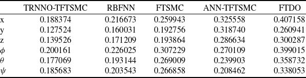
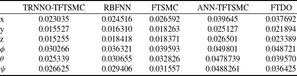
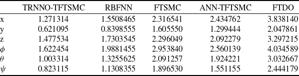
To further illustrate the performance of the TRNNO-TFTSMC method, two error-related performance indices (IAE and ISE) are employed for comparative analysis. Figure 8 presents the histograms of the two error terms, where subfigure (a) shows the comparison of IAE, and subfigure (b) depicts the comparison of ISE. The comparative results clearly demonstrate that all six error terms of the proposed control scheme are the smallest, which directly evidences that the proposed method achieves more stable control performance.
(a) Integral absolute error (IAE). (b) Integral square error (ISE).

(a) Quadrotor position (X, Y, Z). (b) Quadrotor attitude (
 $ \phi, \theta, \psi $
).

The desired and real trajectory of the quadrotor.

5.1.2 Case (b): take the value of
$ 25\mathit{d}$
as the external disturbance

To more intuitively demonstrate the anti-interference capability of the proposed control scheme, the external disturbance is replaced with
 $ 25{d}_{i}=25rsin(\pi t/0.02),(\forall i=x,y,z,\phi, \theta, \psi )$
in this section. With the same desired trajectory, the simulation results of Case (b) are shown in Figs 9(a)–10. As shown in Fig. 9(a) and (b), under larger external disturbances, the TRNNO-TFTSMC method provides faster convergence compared to the other methods. Through the comparison of the zoomed-in plots, it can be clearly observed that after the convergence of the flight system, the steady-state error resulting from the proposed scheme is significantly smaller than that of the other control schemes. This result strongly demonstrates that even in the presence of large external disturbances, the proposed control strategy is capable of achieving accurate and effective control, thereby ensuring the global stability of the flight system. Figure 10 illustrates the 3D trajectory of the quadrotor UAV under large external disturbances. A comparative analysis clearly reveals that while the flight trajectories of other schemes exhibit significant deviations and fluctuations, the proposed control scheme consistently maintains smooth and accurate trajectory tracking. These results fully validate the excellent robustness and dynamic response capability of the proposed control strategy under strong disturbance conditions, further highlighting its engineering application potential in complex flight scenarios.
In this analysis, each position and attitude error term was re-evaluated based on the IAE criterion, with the results summarised in Tables 5–7. As shown in Table 5, the TRNNO-TFTSMC scheme significantly reduces the cumulative error throughout the entire regulation process compared to the other four control schemes under the IAE metric. This indicates that the proposed scheme exhibits appropriate damping characteristics and favourable transient response, effectively suppressing steady-state errors and thereby enhancing control precision. Specifically, compared to the RBF neural network-based method, the TRNNO-TFTSMC achieves a reduction in error fluctuation of approximately 13.02; relative to the conventional FTSMC, the reduction is about 31.62%; in comparison with the ANN-TFTSMC method, the reduction reaches approximately 38.27%; and when contrasted with the FTDO, the proposed approach demonstrates even lower error fluctuation, achieving a reduction of approximately 49.19%. Table 6 summarises the ISE performance metrics for each position and attitude channel. This metric intuitively reflects the sensitivity of the quadrotor aircraft to large errors during the initial response phase. The comparative results demonstrate that the TRNNO-TFTSMC scheme achieves the lowest ISE values among all compared approaches, confirming its superior dynamic response capability in rapidly suppressing large initial deviations. Table 7 summarises the integral time absolute error (ITAE) performance metrics. This indicator intuitively reflects the sensitivity of the quadrotor aircraft to minor errors during the later stages of the response. The comparative results demonstrate that the TRNNO-TFTSMC scheme achieves the smallest ITAE values among all compared methods, confirming its superior stability throughout the system dynamic process.
The analysis results of the aforementioned comparative data indicate that the improvements introduced by the TRNNO-TFTSMC scheme to the system are comprehensive. Its superiority is reflected in both position control accuracy and attitude control accuracy, rather than being confined to a single channel.
5.2 Analysis of experimental feasibility
Based on the proposed TRNNO-TFTSMC scheme and the simulation experiments described above, the analysis of experimental feasibility can be summarised in the following aspects:
-
• The proposed sliding mode control scheme exhibits strong robustness against system parameter perturbations and model uncertainties, making it highly suitable for quadrotor UAVs, which are strongly coupled underactuated systems.
-
• Sinusoidal disturbances with random amplitudes are introduced in the simulation, and disturbance amplification tests (by a factor of 25) are conducted, demonstrating that the controller can effectively cope with uncertain disturbances encountered in actual flight.
-
• A more saturated and smoother tanh function-based control logic is adopted in the experiment, which effectively reduces chattering and mitigates physical actuator tremors during quadrotor UAV flight.
-
• The neural network control logic is optimised, with initial weights selected as small values to prevent drastic control inputs during the initial stage when stabilising the airframe.
-
• Through feedforward compensation by the disturbance observer, the neural network approximation error is reduced while the robustness in actual flight is enhanced.
Comparative analysis of IAE

Comparative analysis of ISE

Comparative analysis of ITAE

5.3 Practical implementation platform
This note describes an experimental validation programme for the proposed control methodology. To validate and test the proposed scenario, we have compiled a complete list of required equipment and, based on this, established a drone test bench. The UAV experimental platform’s hardware configuration is illustrated in Fig. 11. It is a quadrotor of version X450 based on the CUAV V5+ flight control system and is equipped with a ground control station (GCS). The flight control system is based on the STM32F765 as the main functional mock-up unit (FMU) processor, integrates a 6-axis inertial measurement unit (IMU) (including a 3-axis gyroscope and a 3-axis accelerometer), a magnetometer and a barometer. Velocity and position in the horizontal plane are measured by the Global Positioning System (GPS) module and transmitted to the flight control system. The quadrotor system is powered by a lithium-polymer battery pack and governed by a remote control. In addition, GCS ensures communication with the quadrotor via Gigabit Power over Ethernet (PoE). Wind disturbances are generated by a fan and introduced to the quadrotor system to evaluate its disturbance rejection capabilities. Finally, actuators execute the flight controller’s commands, driving the propellers to generate the required aerodynamic forces for achieving the specified flight state.
The quadrotor’s hardware structure.

Remark. Although the aforementioned implementation platform has been successfully established, it still possesses certain inherent limitations compared to real flight testing environments. (i) In actual flight experiments, the flight state information of quadrotor UAVs relies on sensors for data acquisition. Therefore, incorporating sensor faults into consideration is a crucial step for ensuring the reliability of the control scheme. (ii) The simulation experiments are based on the ideal algebraic mapping between control input and the square of motor speed. However, in practical systems, the dynamic response delay of motors and propellers is an unavoidable non-ideal characteristic. (iii) The STM32F765 operates at a main frequency of up to several hundred MHz, necessitating a re-evaluation of whether the computational load imposed by the TRNN algorithm remains within its carrying capacity.
6.0 Conclusion
This paper proposes a novel TRNNO-TFTSMC scheme for a quadrotor UAV flight system subject to nonlinear dynamics and external disturbances. A two-stage sliding mode controller, which employs the hyperbolic tangent function to replace the sign function, is designed to achieve fast convergence of the flight control system states. Simulation results verify that the proposed strategy not only ensures rapid convergence but also significantly attenuates control chattering. In addition, a novel TRNN architecture is proposed to approximate the unknown nonlinear dynamics present in the system, and the adaptive weights of the network are dynamically adjusted based on real-time data, thereby ensuring that the system maintains stability under varying operating conditions. The application of a finite-time observer estimates the approximation error of the TRNN and external disturbances, effectively enhancing the tracking accuracy of the quadrotor UAV and further realising the robust performance of the system. The superiority of the proposed control method has been fully validated through comprehensive multi-scheme and multi-perspective comparisons. Based on the practical experimental platform, future work will focus on applying the control scheme to real-world scenarios to evaluate its control performance under practical operating conditions and explore its potential engineering applications.
Competing interests
We declare that we have no financial and personal relationships with other people or organisations that can inappropriately influence our work. There is no professional or other personal interest of any nature or kind in any product, service and/or company that could be construed as influencing the position presented in, or the review of the manuscript.

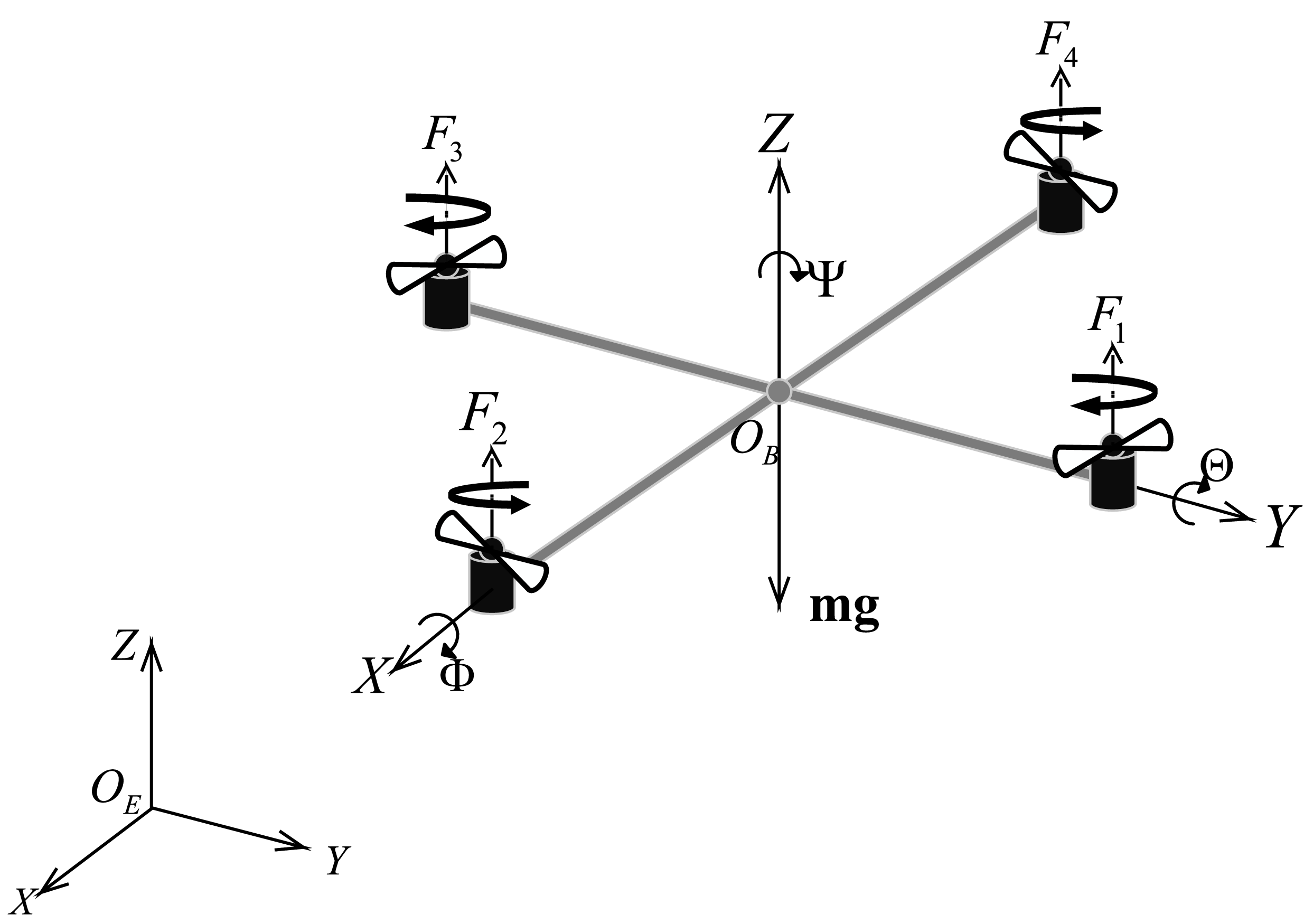


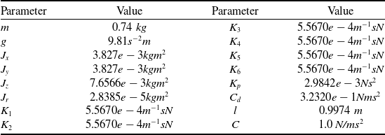
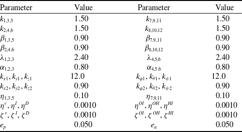
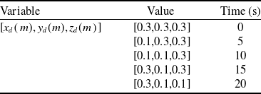
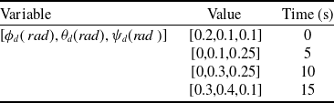

 x,y,z
 ϕ,θ,ψ

 ex,ey,ez
 eϕ,eθ,eψ


 ϕ,θ,ψ