



1. Introduction
Transition from laminar to turbulent flow, commonly classified as natural or bypass scenarios, generally occurs at low and high inflow turbulence levels, respectively. The natural transition process begins with the emergence of two-dimensional (2-D) Tollmien–Schlichting (TS) waves, which undergo progressive amplification and develop into three-dimensional (3-D)
 $\varLambda$
vortex forms before breaking down (Zaki Reference Zaki2013).
The term ‘bypass’, introduced by Morkovin (Reference Morkovin1969), describes a 3-D transition process occurring without the development of TS instabilities (Morkovin Reference Morkovin1969, Reference Morkovin1984). This process, characterised by non-modal growth mechanisms and velocity streaks, is particularly relevant to flows around aircraft wings and turbine blades, where external factors such as surface roughness, acoustic noise or free-stream turbulence can significantly affect the boundary-layer behaviour. Understanding the mechanisms leading to bypass transition is crucial for improving the design and efficiency of aerodynamic surfaces. In the early stages, external disturbances interact with base shear profiles to generate elongated streamwise velocity streaks downstream via the lift-up mechanism. Klebanoff et al. (Reference Klebanoff, Tidstrom and Sargent1962) first observed these coherent structures, noting alternating longitudinal high- and low-velocity streaks that do not align with the linear theory of 2-D TS waves. Kendall (Reference Kendall1985) visualised the flow in a boundary layer subjected to free-stream turbulence with an intensity ranging from 1
 $\,\%$
to 6
 $\,\%$
, and identified slender flow structures of narrow spanwise scale, terming them Klebanoff modes. Andersson et al. (Reference Andersson, Berggren and Henningson1999) revealed that parallel inviscid shear flows are unstable to a broad range of initial infinitesimal 3-D disturbances, explaining the development of longitudinal streaky structures in shear flows. Overall, owing to the complex fluid dynamics involved in bypass transition, most previous studies have focused on flow over a flat plate with a sharp leading edge or zero-pressure-gradient boundary layers.
In contrast, flow around an airfoil with a blunt leading edge has received far less attention. He et al. (Reference He, Gioria, Pérez and Theofilis2017) examined initial perturbation developments in an airfoil flow at relatively low Reynolds numbers and high angles of attack featuring massive separation. Their global linear modal analysis identified that the 2-D Kelvin–Helmholtz (KH) mode in the wake is the most unstable one, whilst the 3-D stationary mode is linked to the laminar separation bubble. Further, their non-modal analysis revealed that the 2-D optimal initial perturbations present substantial transient growth, evolving into the structure of the KH mode over time. In a follow-up study considering the ground effect, He et al. (Reference He, Pérez, Yu and Li2019) demonstrated that ground clearance critically determines the transition from convective to absolute instability in the wake, enhances the energy gain of optimal perturbations and enables the generation of coherent structures in separated flow at low Reynolds numbers. In the canonical massively separated flow, e.g. cylinder flow, wake instability generally governs vortex shedding (Blackburn & Henderson Reference Blackburn and Henderson1999; Meneghini et al. Reference Meneghini, Carmo, Tsiloufas, Gioria and Aranha2011). Similarly, the development of coherent structures in an airfoil wake reveals characteristic flow patterns such as vortex roll-up from separated shear layers and vortex shedding (Yarusevych et al. Reference Yarusevych, Sullivan and Kawall2009). While these findings are insightful for high-incidence conditions, many practical applications of airfoil flow are at low to moderate angles of attack. The work by Gupta et al. (Reference Gupta, Zhao, Sharma, Agrawal, Hourigan and Thompson2023) established the parameter dependence of various states in a NACA0012 airfoil flow, explicitly showing that the flow remains globally stable over a broad range of low to moderate angles of attack. However, these flows are sensitive to continuous inflow disturbance, which undergoes significant amplification and would lead to bypass transition as observed in flat-plate boundary-layer flow (Andersson et al. Reference Andersson, Berggren and Henningson1999; Brandt et al. Reference Brandt, Schlatter and Henningson2004; Huang et al. Reference Huang, Xiao, Ren, Wang, Xi and Mao2021).
In terms of algorithms, wake instability can be analysed using asymptotic instability theory, while the lift-up mechanism entails a non-modal transient growth process related to the linear optimal perturbation theory. Farrell (Reference Farrell1988) first introduced the concept of an optimal initial disturbance that yields the largest growth over a given time horizon, proposing that such transient growth of small disturbances can trigger nonlinear processes that eventually lead to the transition to turbulence. Generally, there are two approaches to calculating the optimal initial perturbation: eigenvalue and variational optimisation methods, which are equivalent in the linear regime and require iterative solutions of the linearised Navier–Stokes (NS) and adjoint equations. The eigenvalue method identifies the optimal perturbation as the eigenvector associated with the leading eigenvalue of a joint operator, typically extracted from a Krylov sequence using the Arnoldi method (Arnoldi Reference Arnoldi1951). Using this approach, Andersson et al. (Reference Andersson, Berggren and Henningson1999) calculated the optimal upstream disturbances, which consist of streamwise vortices developing into streamwise streaks. In the variational method, the optimal perturbation is regarded as the velocity vector that maximises a constrained Lagrangian function. Luchini (Reference Luchini2000) defined and calculated the optimal disturbances of a flat-plate boundary layer driven by the lift-up mechanism at various spanwise wavenumbers. Similar research has examined optimal streamwise amplification in the Blasius boundary layer (Monokrousos et al. Reference Monokrousos, Åkervik, Brandt and Henningson2010), showing that the lift-up mechanism is dominant, and the perturbation changes from streamwise vorticity to streamwise elongated streaks in the downstream direction over short optimisation intervals.
Given that the free-stream turbulence is continuous, inflow perturbations are more pertinent to bypass transition in airfoil flows than initial perturbations. An adjoint variational algorithm to compute the optimal boundary perturbation, namely the most amplified one by the base flow, has been developed. This algorithm incorporates both optimisation and eigenvalue approaches, analogous to those employed for initial condition problems (Mao et al. Reference Mao, Blackburn and Sherwin2013). Applying these algorithms, Wang et al. (Reference Wang, Mao and Zaki2019) computed the optimal inflow perturbation for flow over a flat plate with a sharp leading edge, and Xiao et al. (Reference Xiao, Zhang, Sun and Mao2022) extended this analysis to the weakly nonlinear regime. In the present work, the optimal inflow perturbation is computed for flow over a NACA0012 airfoil with a blunt leading edge. This configuration, previously unexplored in optimal inflow studies, is more relevant to engineering applications than flows with sharp or no leading-edge configurations. The work aims to elucidate the effects of the blunt leading edge and inform strategies for predicting and controlling transitional flow. For example, this knowledge can guide the installation of sensors by identifying critical locations where monitoring the frequency and wavenumber spectrum of perturbations is essential.
Beyond linear mechanisms associated with the formation and amplification of streaks, understanding the nonlinear evolution leading to breakdown is key to predicting transition. In the nonlinear lift-up process, low-speed streaks are lifted above the high-speed ones, leading to a shear profile prone to secondary instabilities (Asai et al. Reference Asai, Minagawa and Nishioka2002). Both varicose and sinuous instabilities can be identified corresponding to spanwise symmetric and antisymmetric deformations of streaks, respectively (Vaughan & Zaki Reference Vaughan and Zaki2011). The varicose mode is characterised by in-phase oscillations of streaks, while the sinuous mode features out-of-phase undulations, as illustrated in the stability analyses of boundary-layer streaks (Andersson et al. Reference Andersson, Brandt, Bottaro and Henningson2001) and Görtler vortices (Bottaro & Klingmann Reference Bottaro and Klingmann1996). However, high Reynolds numbers are required to trigger such a significant nonlinear process, and the optimal inflow perturbation is difficult to calculate under these conditions. Matsubara & Alfredsson (Reference Matsubara and Alfredsson2001) experimentally revealed that, under free-stream turbulence, streak scales are set by the boundary-layer thickness, and hence the Reynolds number. This correlation provides a basis for projecting the optimal perturbation obtained at low Reynolds numbers to higher ones.
In the rest of this paper, the theoretical methodology based on the adjoint variational method to compute the optimal inflow perturbation is presented in § 2. The computation set-up is described in § 3. The results are reported in § 4 with the linear optimal energy gain displayed in § 4.1, typical modes discussed in §§ 4.2 and 4.3, the dynamics associated with the lift-up mechanism delineated in § 4.4 and the nonlinear evolution process exhibited in § 4.5. Finally, a conclusion is drawn in § 5.
2. Methodology
2.1. Governing equations
Considering the incompressible flow around the NACA0012 airfoil, the governing NS equations are
 \begin{equation} \partial _t{\boldsymbol{u}}{{ = - }}{\boldsymbol{u}}\, \boldsymbol{\cdot }\,{\boldsymbol{\nabla }} {\boldsymbol{u}} - {\boldsymbol{\nabla }}\! p + {{\mathop {Re}\nolimits } ^{ - 1}}{\nabla} ^2{\boldsymbol{u}}, \quad {\boldsymbol{\nabla }} \boldsymbol{\cdot }{\boldsymbol{u}} = 0, \end{equation}
where
 $t$
is time,
 ${\boldsymbol{u}} =(u,v,w)^{\mathrm{T}}$
is the non-dimensional velocity vector and
 $p$
is the pressure. Here,
 $u$
,
 $v$
and
 $w$
are the streamwise, wall-normal and spanwise velocity components, respectively. The Reynolds number
 ${\mathop {{Re}}\nolimits } \equiv U_\infty c/ \nu$
is based on the free-stream velocity
 $U_\infty$
, the chord length
 $c$
and the fluid viscosity
 $\nu$
.
The flow can be decomposed as the sum of a base state, which is a 2-D steady solution of (2.1), and a perturbation
 \begin{equation} ({\boldsymbol{u}}, p) = ({\boldsymbol{U}}, P) + ({\boldsymbol{u}}', p'), \end{equation}
where (
 $\boldsymbol{U}$
, P) and (
 ${\boldsymbol{u}}'$
, p
 $'$
) denote the base and the perturbation fields, respectively. The components of the perturbation velocity are correspondingly denoted as
 ${\boldsymbol{u}}'$
=
 $(u', v', w')^{\mathrm{T}}$
.
The linearised NS equations that govern the evolution of perturbations are obtained by substituting (2.2) into (2.1) and neglecting the nonlinear second-order term
 \begin{equation} \partial _t{\boldsymbol{u}}'{\mathrm{\, = \,}} - \,{\boldsymbol{U}} \boldsymbol{\cdot }\,{\boldsymbol{\nabla }} {\boldsymbol{u}}'\, - ({\boldsymbol{\nabla }} {\boldsymbol{U}})^{\mathrm{T}} \boldsymbol{\cdot }{\boldsymbol{u}}' - {\boldsymbol{\nabla }}\! p' + {{\mathop {Re}\nolimits } ^{ - 1}}{\nabla} ^2{\boldsymbol{u}}', \quad {\boldsymbol{\nabla }} \boldsymbol{\cdot }{\boldsymbol{u}}' = 0. \end{equation}
The perturbation can be further represented by a Fourier expansion in the spanwise direction under 3-D conditions
 \begin{equation} \boldsymbol{u}'(x,y,z,t) = \mathcal{R}\left \{\sum \limits _{\beta = 0}^\infty \boldsymbol{u}{'_\beta } (x,y,t){e^{i\beta z}}\right \}\!, \end{equation}
where
 $\mathcal R \left \{ \right \}$
defines the real part,
 $\beta$
denotes the spanwise wavenumber and
 $x$
,
 $y$
and
 $z$
are coordinates in the streamwise, wall-normal and spanwise directions, respectively. Under the linear assumption, each spanwise wavenumber
 $\beta$
can be analysed independently. In the rest of this paper,
 ${\boldsymbol{u}}'$
is used to represent the perturbation at a specific spanwise wavenumber for simplicity.
2.2. Linear optimal inflow perturbation
The free-stream or inflow perturbation depends on both time and space, and under the linear assumption, it can be represented as
 \begin{equation} \boldsymbol{u}'(\boldsymbol{x}_{\textit{in}}, t) = G(t){\boldsymbol{u}}_{\textit{in}}'(\boldsymbol{x}_{\textit{in}}), \end{equation}
where
 ${\boldsymbol{x}}_{\textit{in}}$
denotes the inflow boundary coordinates and
 ${\boldsymbol{u}}_{\textit{in}}'({{\boldsymbol{x}}_{\textit{in}}})$
is the spatial form of the inflow perturbation. Here, G(t) is a function that defines the temporal dependence given by
 \begin{equation} G(t) = \big(1 - {e^{ - \sigma {t^2}}}\big)\big(1 - {e^{ - \sigma {{(\tau - t)}^2}}}\big){e^{i\omega t}}, \end{equation}
where
 $\sigma$
is a relaxation factor to ensure the inflow perturbation is zero at
 $\textit {t} = 0$
and
 $\textit {t} = \tau$
, eliminating the temporal discontinuities at the beginning of the integration of the linearised NS equations (2.3) and adjoint equations, as required by the optimisation algorithm (Mao et al. Reference Mao, Blackburn and Sherwin2013). A large value of
 $\sigma$
is preferred to mitigate the impact of the relaxation (i.e. the modulation of the first two terms to the last one in (2.6)) and
 $\sigma = 100$
is adopted here as used in previous works (Wang et al. Reference Wang, Mao and Zaki2019; Xiao et al. Reference Xiao, Zhang, Sun and Mao2022). It has been verified that the distribution of the optimal perturbations remains unchanged with further increase of
 $\sigma$
. The parameter
 $\tau$
is the optimisation time and is set to 4 if not otherwise stated. This time interval is sufficient to reveal the mechanisms of perturbations, as will be demonstrated in § 3. The last term in (2.6) specifies the frequency
 $\omega$
of the free-stream perturbation and can be considered as a Fourier decomposition when neglecting the relaxation effects.
By definition, the optimal inflow perturbation maximises the energy gain at a specific frequency over the optimisation time. Consequently, the energy gain can be measured in terms of the ratio of the energy at the final time to that of the inflow perturbation
 \begin{equation} K = \frac {{\int \limits _\varOmega {W\boldsymbol{u}'(\tau ) \boldsymbol{\cdot }\,} \boldsymbol{u}'(\tau ){\mathrm{d}}\varOmega }}{E_{\textit{in}}}, \quad \mathrm{ with} \quad {E_{\textit{in}}} = \int \limits _{S} {\boldsymbol{u}_{\textit{in}}^{^\prime } \boldsymbol{\cdot }\,} \boldsymbol{u}_{\textit{in}}^{^\prime }{\mathrm{d}}S, \end{equation}
where
 $S$
and
 $\varOmega$
denote the inflow boundary and computational domain, respectively, and
 $W$
is a weight function set to
 $1$
unless otherwise stated. To maximise the objective function in (2.7) while satisfying the linearised governing equations, a Lagrangian
 $\mathcal L$
is defined as
 \begin{align} \mathcal{L} = K &- \frac {1}{\tau } \int \limits _0^\tau \int \limits _\varOmega \Bigl \{ \boldsymbol{u}^* \boldsymbol{\cdot }\Bigl [ \partial _t \boldsymbol{u}' + \boldsymbol{U} \boldsymbol{\cdot }{\boldsymbol{\nabla }} \boldsymbol{u}' + (\boldsymbol{\nabla } \boldsymbol{U})^{\mathrm{T}} \boldsymbol{\cdot }\boldsymbol{u}' \nonumber \\ &\quad + \boldsymbol{\nabla } p' - {\mathop {Re}}^{-1} {\nabla} ^2 \boldsymbol{u}' \Bigr ] + p^* (\boldsymbol{\nabla } \boldsymbol{\cdot }\boldsymbol{u}') \Bigr \} \, \mathrm{d}\varOmega \, \mathrm{d}t, \end{align}
where
 ${\boldsymbol{u}}^*$
and
 $\textit {p}^*$
stand for the adjoint velocity and pressure, respectively. The flow variables in the second term of (2.8) satisfy the governing equations as constraints.
A stationary point of the Lagrangian can be sought by setting its variation with respect to variables (
 ${\boldsymbol{u}}'$
,
 $p'$
) to zero. Through integration by parts, a set of adjoint equations can be obtained
 \begin{equation} \partial _t {\boldsymbol{u}^*} + {\boldsymbol{U}} \boldsymbol{\cdot }{\boldsymbol{\nabla }} {\boldsymbol{u}^*} - {\boldsymbol{\nabla }} {\boldsymbol{U}} \boldsymbol{\cdot }{\boldsymbol{u}^*} - {\boldsymbol{\nabla }}\! {p^*} + {{\mathop {Re} \nolimits } ^{ - 1}}{\nabla} ^2{\boldsymbol{u}^*} = 0, \,\quad {\boldsymbol{\nabla }} \boldsymbol{\cdot }{\boldsymbol{u}^*} = 0, \end{equation}
which should be integrated backwards in time from
 $\textit {t} = \tau$
to
 $\textit {t} = 0$
with an initial condition
 ${{\boldsymbol{u}}_\tau ^{*}} = 2\tau W{{\boldsymbol{u}}_\tau ^{^\prime }}$
(Barkley et al. Reference Barkley, Blackburn and Sherwin2008). Regarding the boundary conditions for (2.3) and (2.9), at the inflow, the velocity vector satisfies Dirichlet conditions, while a zero Dirichlet condition is imposed on the adjoint velocity. On the outflow boundary, the forward equations retain a typical zero-Neumann condition
 $(\boldsymbol{\nabla }_{\!{n}} \boldsymbol{u} = 0,\ p = 0)$
. For the backward integration of the adjoint equations, a Robin condition derived from the variational derivation is required as
 ${\boldsymbol{\nabla} }_{\!{n}}{{{\boldsymbol{u}}^*}} + \mathop {Re}{{\boldsymbol{U}}}_{\!{n}}{{\boldsymbol{u}}^*} = 0, \,p^* = 0,$
where
 $\boldsymbol{n}$
denotes the direction normal to the boundary and
 ${\boldsymbol{U}}_{\!{n}}=\boldsymbol {U}\boldsymbol{\cdot }\boldsymbol n$
(Mao et al. Reference Mao, Blackburn and Sherwin2013).
The gradient of the energy gain with respect to the inflow perturbation is then obtained
 \begin{equation} {\boldsymbol{\nabla }_{\boldsymbol{u}_{{in}}^{^\prime }}}K = \frac {1}{\tau }\int \limits _0^\tau {\big ( {{p^*}\boldsymbol{n} - {{{\mathop {Re}\nolimits } }^{ - 1}}{\boldsymbol{{\boldsymbol{\nabla }}} _{\!{n}}}\boldsymbol{u}^*} \big)} G\mathrm{d}t. \end{equation}
Equation (2.10) is then applied to update the inflow perturbation iteratively until convergence is achieved
 \begin{equation} \boldsymbol{u}_{\textit{in}}^{^\prime k + 1} = \boldsymbol{u}_{\textit{in}}^{^\prime k} + a \,{\boldsymbol{\nabla }}_{\boldsymbol{u}_{\textit{in}}^{^\prime }}K, \end{equation}
where
 $k$
is the iteration step and
 $a$
is the step length, with its optimal value determined through an analytical optimisation process by exploiting the linear feature of the governing equations. The optimisation procedure for computing the optimal inflow perturbation is summarised as follows:
-
(i) Evolve an initial guess of the optimal inflow perturbation
 ${\boldsymbol{u}}_{\textit{in}}^{^\prime }$
by integrating equations (2.3) forwards from
$\textit {t} = 0$
to
$\textit {t} = \tau$
.
-
(ii) Scale
${\boldsymbol{u}}_\tau ^{^\prime }$
to obtain the initial condition of the adjoint equations
${\boldsymbol{u}}_\tau ^{*}$
. -
(iii) Evolve
${\boldsymbol{u}}_\tau ^{*}$
using (2.9) to obtain
${\boldsymbol{u}}^{*}$
and
$p^*$
by integrating the adjoint velocity backwards from
$\textit {t} = \tau$
to
$\textit {t} = 0$
. -
(iv) Solve (2.10) to obtain
${\boldsymbol{\nabla } _{\kern-1pt\boldsymbol{u}_{{in}}^{^\prime }}}K$
. -
(v) Update the inflow perturbation from step
$k$
to
$k+1$
using (2.11). -
(vi) Terminate if convergence is achieved. Otherwise, return to step 2.


3. Computational set-up
Simulations of flow past a NACA0012 airfoil are conducted on a computing platform that has been widely used and verified in studies of flow around a flat plate with a sharp leading edge (Wang et al. Reference Wang, Mao and Zaki2019; Huang et al. Reference Huang, Xiao, Ren, Wang, Xi and Mao2021; Xiao et al. Reference Xiao, Zhang, Sun and Mao2022), pulsatile flow in stenosis (Mao et al. Reference Mao, Blackburn and Sherwin2012) and flow past a backward-facing step (Mao Reference Mao2015). The full computational domain of the flow field shown in figure 1 spans from
 $x = -2$
to
 $x = 200$
and
 $y = -40$
to
 $y = 40$
in the streamwise and wall-normal directions, respectively. The leading edge of the NACA0012 airfoil is located at
 $(x, y) = (0, 0)$
. The chord length
 $c$
and free-stream velocity
 $U_\infty$
are used as the reference length and velocity, respectively.
Schematic diagram of the full computational domain and boundary conditions.

The spectral element method is adopted to solve the NS, linearised NS and adjoint equations. These equations are discretised into 7803 spectral elements in the
 $x{-}y$
plane, with a wavenumber assigned in the spanwise direction as shown in (2.4). To resolve the flow details accurately, the mesh points are clustered around the airfoil and near the inflow boundary, as shown in figure 2. Each element is further divided into a
 $(N+1) \times (N+1)$
grid, where
 $N$
is a polynomial order that denotes the spatial order of discretisation.
Computational mesh around (a) the full domain, (b) the airfoil and (c) the inflow boundary.

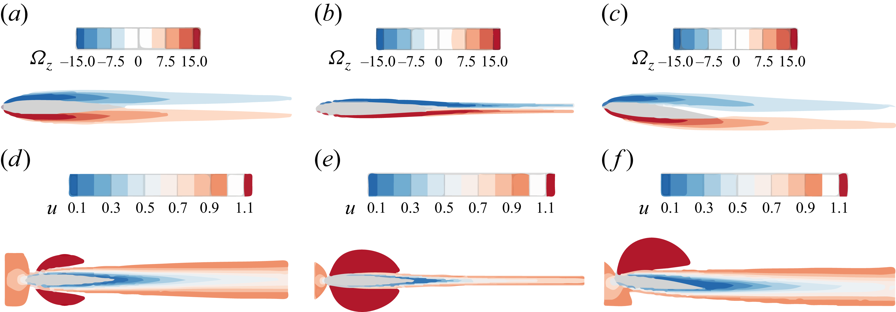
Dirichlet boundary conditions are imposed at the inflow, and far-field conditions are applied on the upper and lower sides of the domain. The 2-D base flow is computed by solving (2.1) to obtain a steady solution. Contours of the spanwise vorticity
 $\varOmega _z$
and streamwise velocity
 $u$
fields at
 $\textit{Re} = 1000$
and
 $\textit{Re} = 8000$
, with an angle of attack
 $\alpha = 0^{\circ }$
and 6
 $^{\circ }$
, are displayed in figure 3. The flow around the NACA0012 airfoil remains steady over the parameters studied. Symmetrical shear layers develop on both sides of the airfoil when
 $\alpha = 0^{\circ }$
and become thinner and shorter at higher
 ${\textit{Re}}$
. Increasing
 ${\textit{Re}}$
or
 $\alpha$
promotes flow unsteadiness, and downstream of the airfoil, the detached shear layers generate a wake velocity profile with an inflection point, which is indicative of flow instability. Additionally, the flow wraps around the airfoil and begins to separate from the trailing edge.
Base flow at
 $(\alpha , \textit{Re}) = (0^{\circ }, 1000), (0^{\circ }, 8000), (6^{\circ }, 1000)$
from left to right. The upper and lower rows are contours of the spanwise vorticity and streamwise velocity, respectively.

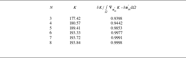
Convergence of the gain
 $K$
with respect to the polynomial order
 $N$
at
 $\alpha = 0^{\circ }$
,
 ${\textit{Re}} = 8000$
,
 $\beta = 25$
and
 $\omega = 0$
.

Table 1. Long description
A table with three columns and six (rows excluding header) rows. The columns are labeled N, K, and δK / ∫_Ω (∇_u’ · K · δu’) dΩ. The rows present the following data: Row 1: N, 3; K, 177.42; δK / ∫_Ω (∇_u’ · K · δu’) dΩ, 0.9398. Row 2: N, 4; K, 180.57; δK / ∫_Ω (∇_u’ · K · δu’) dΩ, 0.9442. Row 3: N, 5; K, 189.41; δK / ∫_Ω (∇_u’ · K · δu’) dΩ, 0.9853. Row 4: N, 6; K, 193.33; δK / ∫_Ω (∇_u’ · K · δu’) dΩ, 0.9977. Row 5: N, 7; K, 193.72; δK / ∫_Ω (∇_u’ · K · δu’) dΩ, 0.9991. Row 6: N, 8; K, 193.84; δK / ∫_Ω (∇_u’ · K · δu’) dΩ, 0.9998.
To assess the convergence of the numerical method when solving the perturbation equations, table 1 shows the energy gain
 $K$
for the optimal inflow perturbation in the second column at the highest
 ${\textit{Re}}$
considered in the calculation, i.e.
 ${\textit{Re}} = 8000$
with
 $\alpha = 0^\circ$
,
 $\beta = 25$
and
 $\omega = 0$
for different polynomial orders. In the third column, the deviation of the value from unity represents the error in the calculation of the gradient (see (2.10)). The results indicate that
 $N = 6$
is sufficient to ensure convergence and is consequently adopted in the following simulations. The convergence of the optimisation process is also performed, and a consistent convergence of the optimal perturbation (i.e. within
 $0.1\,\%$
) can be reached within 5–6 iterations.
The discretisation described above is used for the linear optimal perturbation analysis. For the nonlinear direct numerical simulation (DNS) at
 ${\textit{Re}} = 100\,000$
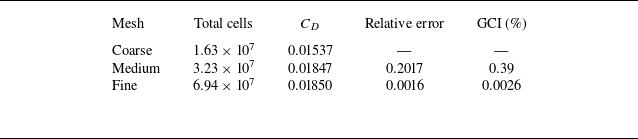
, a well-resolved finite-volume discretisation is employed to capture the transition process. Grid refinement is applied near the wall and around the leading edge to resolve boundary-layer development and streak evolution, while the spanwise direction is treated as periodic. Three systematically refined meshes are used, and the corresponding results are summarised in table 2. The mean drag coefficient
 $C_D$
converges monotonically with mesh refinement. The relative error between successive grids is defined as the absolute difference in
 $C_D$
divided by the value on the coarser grid. This error is
 $20.17\,\%$
for the coarse–medium-grid pair and
 $0.16\,\%$
for the medium–fine-grid pair. A grid convergence index (GCI) analysis (Roache Reference Roache1994) yields GCI values of
 $0.39\,\%$
for the medium grid and
 $0.0026\,\%$
for the fine grid, indicating that the fine-grid solution is sufficiently grid converged for the present DNS analysis. Accordingly, the fine grid is used for all nonlinear simulations in § 4.5.
Grid convergence results for DNS at
 ${\textit{Re}}=100\,000$
.

Table 2. Long description
The table presents grid convergence results for direct numerical simulation at a specific condition. It has five columns and three rows (rows excluding header). The columns are labeled Mesh, Total cells, C D, Relative error, and GCI (percent). The rows are labeled Coarse, Medium, and Fine. Row 1: Mesh, Coarse; Total cells, 1.63 times 10 to the power of 7; C D, 0.01537; Relative error, blank; GCI (percent), blank. Row 2: Mesh, Medium; Total cells, 3.23 times 10 to the power of 7; C D, 0.01847; Relative error, 0.2017; GCI (percent), 0.39. Row 3: Mesh, Fine; Total cells, 6.94 times 10 to the power of 7; C D, 0.01850; Relative error, 0.0016; GCI (percent), 0.0026.
Further, to assess the influence of the optimisation time horizon, various values, i.e.
 $\tau =4, 10, 20, 30$
and 40, are tested. Either
 $\beta =0$
or
 $\omega =0$
is adopted in this test since they represent the critical scenarios, as will be illustrated in § 4. As shown in figure 4, the energy gain at the final optimisation time
 $K(\tau )$
presents similar trends for different
 $\tau$
, illustrating that the mechanism of perturbation growth can be captured robustly over the values of
 $\tau$
considered, and the growth saturates at
 $\tau =30$
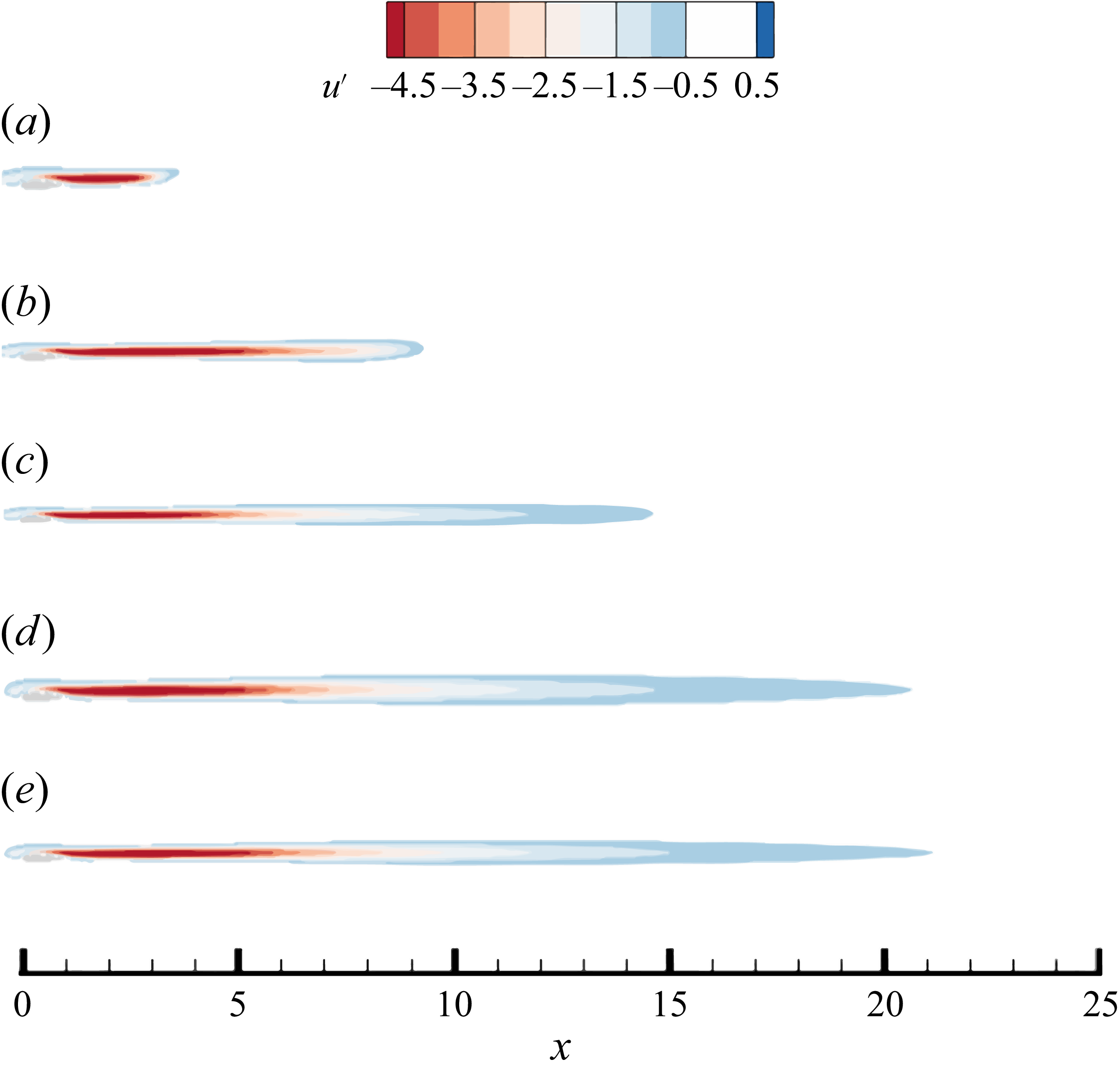
. To confirm this observation, the form of the outcome of perturbation is checked. For clarity, throughout this paper, the real part of optimal perturbations will be illustrated only. As shown in figure 5, the 2-D unsteady mode is with essentially the same spatial pattern but just extends further downstream when
 $\tau$
increases. Similar behaviour can be observed for the 3-D steady mode (see figure 6). Therefore, it can be concluded that the fundamental pathway of perturbation amplification can be robustly captured at
 $\tau =4$
, and a further increase of
 $\tau$
only allows for longer downstream development away from the airfoil.
Optimal gain
 $K(\tau )$
at the final optimisation time for different
 $\tau$
at
 $\alpha = 0^{\circ }$
,
 ${\textit{Re}}=1000$
and (a)
 $\omega = 0$
and (b)
 $\beta = 0$
.

Contours of the spanwise vorticity of the optimal outcome at
 $\alpha = 0^{\circ }$
,
 ${\textit{Re}}=1000$
,
 $\omega = 6$
,
 $\beta =0$
and
 $t=\tau =4, 10, 20,30$
and 40, for (a), (b), (c), (d) and (e), respectively.

Figure 5. Long description
Panel A: A heat map showing the spanwise vorticity of the optimal outcome at a specific value. The x-axis ranges from 0 to 30, and the y-axis represents the spanwise vorticity values ranging from -20 to 20. The color scale indicates the intensity of vorticity, with red representing lower values and blue representing higher values. The vorticity pattern shows a series of alternating red and blue regions, indicating areas of low and high vorticity. Panel B: A heat map showing the spanwise vorticity of the optimal outcome at a different value. The x-axis ranges from 0 to 30, and the y-axis represents the spanwise vorticity values ranging from -20 to 20. The color scale indicates the intensity of vorticity, with red representing lower values and blue representing higher values. The vorticity pattern shows a more extended series of alternating red and blue regions compared to Panel A. Panel C: A heat map showing the spanwise vorticity of the optimal outcome at another value. The x-axis ranges from 0 to 30, and the y-axis represents the spanwise vorticity values ranging from -20 to 20. The color scale indicates the intensity of vorticity, with red representing lower values and blue representing higher values. The vorticity pattern shows an even more extended series of alternating red and blue regions compared to Panels A and B. Panel D: A heat map showing the spanwise vorticity of the optimal outcome at yet another value. The x-axis ranges from 0 to 30, and the y-axis represents the spanwise vorticity values ranging from -20 to 20. The color scale indicates the intensity of vorticity, with red representing lower values and blue representing higher values. The vorticity pattern shows a highly extended series of alternating red and blue regions compared to Panels A, B, and C. Panel E: A heat map showing the spanwise vorticity of the optimal outcome at the final value. The x-axis ranges from 0 to 30, and the y-axis represents the spanwise vorticity values ranging from -20 to 20. The color scale indicates the intensity of vorticity, with red representing lower values and blue representing higher values. The vorticity pattern shows the most extended series of alternating red and blue regions compared to Panels A, B, C, and D.
Contours of the streamwise velocity of the optimal outcome at
 $\alpha = 0^{\circ }$
,
 ${\textit{Re}}=1000$
,
 $\omega = 0$
,
 $\beta =9$
and
 $t=\tau =4, 10, 20,30$
and 40, for (a), (b), (c), (d) and (e), respectively.

4. Results
4.1. Optimal energy gain
Optimal inflow perturbation analyses are first conducted at
 ${\textit{Re}} = 1000$
, with the angle of attack ranging from
 $\alpha = 0^{\circ }$
to 6
 $^{\circ }$
for various spanwise wavenumbers
 $\beta$
and frequencies
 $\omega$
. The corresponding energy gain in the
 $\beta - \omega$
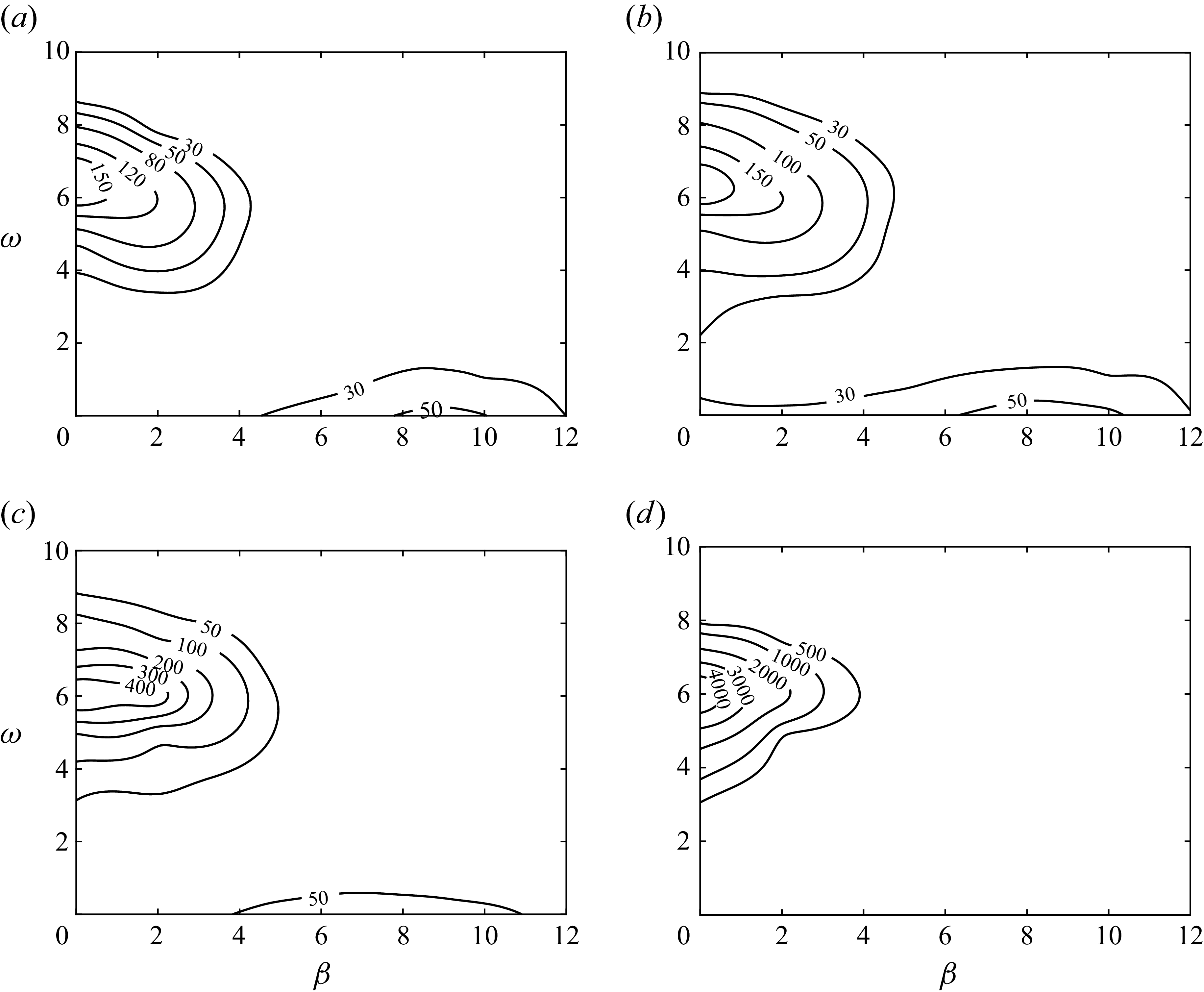
plane is displayed in figure 7. For
 $\alpha = 0^{\circ }$
, two distinct local peaks are observed, one at
 $(\beta , \omega ) = (0, 5.8)$
and the other at
 $(\beta , \omega ) = (9, 0)$
. The former corresponds to a 2-D unsteady mode, whereas the latter represents a 3-D steady mode driven by the lift-up effect. The emergence of the more amplified 2-D mode highlights a fundamental departure from the flat-plate scenario, a difference that stems from the airfoil geometry. As
 $\alpha$
increases, the gain of the first peak (which remains at an almost constant frequency around
 $\omega = 5.8$
) continues to increase. In contrast, the gain of the second peak is always smaller than that of the first and decreases progressively with increasing
 $\alpha$
, becoming nearly negligible at
 $\alpha = 6^{\circ }$
, as shown in figure 7(
 $d$
). In the following sections, we focus on these two distinct modes at different
 ${\textit{Re}}$
.
Contours of the gain of the optimal inflow perturbation at
 ${\textit{Re}} = 1000$
and (a)
 $\alpha = 0^{\circ }$
, (b)
 $\alpha = 2^{\circ }$
, (c)
 $\alpha = 4^{\circ }$
and (d)
 $\alpha = 6^{\circ }$
.

4.2. Two-dimensional mode
Figure 8 presents the velocity profiles of the optimal inflow perturbation for the 2-D unsteady mode, identified at
 $(\beta , \omega ) = (0, 6)$
and
 $\textit{Re} = 1000$
in figure 7. It is observed that the magnitudes of
 $u'$
and
 $v'$
are significantly larger than that of
 $w'$
, indicating an essentially 2-D inflow perturbation with a trivial spanwise component. At
 $\alpha = 0^{\circ }$
, the
 $u'$
component of the velocity is antisymmetric, and the
 $v'$
component is symmetric, with respect to
 $y = 0$
. As
 $\alpha$
increases, the perturbation gradually concentrates on the upper part, suggesting that the upper section of the base flow acts as a stronger amplifier. A further increase in
 $\alpha$
leads to flow separation and even stronger amplification of inflow disturbances.
Velocity profiles of the optimal inflow perturbation at
 ${\textit{Re}} = 1000$
,
 $\omega = 6$
,
 $\beta = 0$
and (a)
 $\alpha = 0^{\circ }$
, (b)
 $\alpha = 2^{\circ }$
, (c)
 $\alpha = 4^{\circ }$
and (d)
 $\alpha = 6^{\circ }$
.

Figure 8. Long description
Panel A: A line graph shows velocity profiles of the optimal inflow perturbation. The x-axis represents u_in’ ranging from -1.0 to 1.5, and the y-axis represents y ranging from -3 to 3. The graph includes three lines: a solid line for u’, a dashed line for v’, and a dotted line for w’. The lines exhibit distinct patterns, with u’ showing sharp peaks and troughs around y = 0, while v’ and w’ display more gradual changes. Panel B: Another line graph with similar axes and line styles. The patterns are slightly different, with u’ still showing sharp peaks but with a broader range. v’ and w’ follow similar trends as in Panel A. Panel C: This line graph also follows the same axis and line styles. The u’ line shows sharp peaks and troughs, while v’ and w’ exhibit gradual changes. Panel D: The final line graph maintains the same axis and line styles. The u’ line shows sharp peaks and troughs, with v’ and w’ displaying gradual changes similar to the previous panels.
The corresponding downstream responses of the flow to the four inflow perturbations are shown as contours of the spanwise vorticity in figure 9. Convectively amplified by the wake profile, these optimal modes are concentrated in the wake region and exhibit a clear spatial periodicity with an approximate streamwise wavenumber of 10, characterising a localised wake instability. Tracing the perturbation from the inflow boundary reveals its evolution: it first decays upstream of the leading edge due to viscous diffusion, grows around the leading edge as the thin shear layer amplifies it, decays again along the airfoil with the base shear (see figure 3), then undergoes a second stage of growth in the wake owing to instability and finally decays downstream as the base shear weakens. Increasing
 $\alpha$
changes the detailed structure of the optimal response but preserves the same overall mechanism.
Contours of the spanwise vorticity at
 ${\textit{Re}} = 1000$
,
 $\omega = 6$
,
 $\beta = 0$
and (a)
 $\alpha = 0^{\circ }$
, (b)
 $\alpha = 2^{\circ }$
, (c)
 $\alpha = 4^{\circ }$
and (d)
 $\alpha = 6^{\circ }$
.

For
 $\alpha = 0^{\circ }$
, the inflow perturbation and base flow are symmetric, as is the disturbance around the airfoil, illustrating an equivalent amplification of perturbations on the upper and lower sides of the airfoil. These disturbances then serve as initial seeds for the wake instability. At higher
 $\alpha$
, both the inflow and the disturbance around the airfoil become asymmetric, exploiting the higher amplification rate on the upper surface. Additionally, the disturbance from the upper shear layer can directly energise the unstable region in the wake, as demonstrated in figure 9(
 $d$
). The present analysis shows that this 2-D unsteady mode undergoes amplification predominantly in the wake, governed by the KH mechanism that was previously identified as the dominant instability in massively separated airfoil flows (He et al. Reference He, Gioria, Pérez and Theofilis2017). This amplification occurs across both separated and attached flow regimes, demonstrating that the KH mechanism can be excited by optimal inflow perturbations over the angle-of-attack range considered here.
The physical origin of this amplification lies in the inflectional nature of the wake velocity profile. As shown in figure 10, the base shear layers attached to the upper and lower surfaces generate a wake profile with an inflection point, marked by the red circles. It is well known that this type of instability is predominantly two-dimensional and inviscid, as dictated by Rayleigh’s theorem (Drazin & Reid Reference Drazin and Reid2004). This instability due to the inflection point is observed consistently over the parameters considered in the present work (e.g.
 $\alpha$
,
 $\omega$
and
 ${\textit{Re}}$
), which aligns with and extends the global instability findings in a NACA0012 airfoil flow at
 $\alpha = 5^{\circ }$
and
 ${\textit{Re}}=1000$
, where the most unstable eigenmode was likewise identified in the wake region (Theofilis et al. Reference Theofilis, Barkley and Sherwin2002). This observation is further supported by the work of Gioria et al. (Reference Gioria, He and Theofilis2015), who explicitly identified the travelling wake mode instability as the global linear instability mechanism, underscoring its prevalence over stationary 3-D modes.
Streamlines of base flow in the region (a) around the airfoil, and (b) in the wake at
 $\alpha = 0^{\circ }$
and
 ${\textit{Re}} = 1000$
.

4.3. Steady mode
We then turn to the second form of the perturbation growth observed in figure 7, i.e. the steady 3-D mode. Since this mode is more amplified at low angles of attack, we focus on the
 $\alpha = 0^{\circ }$
case and explore the effect of the Reynolds number. As shown in figure 11, the gain reaches its global maximum at an optimal value of
 $\beta$
(the case of
 $\beta = 0$
, which corresponds to a local maximum, is not discussed further as it represents a 2-D mode with significantly lower growth than the wake mode). For
 ${\textit{Re}} = 1000, 2000, 5000, 8000$
, the optimal
 $\beta$
values are 9, 13, 21, 25, respectively, illustrating an increasing trend as expected, since the associated flow structures (e.g. the boundary-layer thickness) decrease with increasing
 ${\textit{Re}}$
. The optimal normalised wavenumber, defined as
 $\eta = \beta / {\sqrt {\textit{Re}}}$
, remains approximately constant across this Reynolds number range, taking a value of approximately 0.28. This insensitivity of the normalised wavenumber has also been observed in sharp leading-edge flat-plate flow (Wang et al. Reference Wang, Mao and Zaki2019).
Optimal gain
 $K(\tau )$
at different
 $\beta$
with
 $\alpha = 0^{\circ }$
,
 $\omega = 0$
,
 $\tau =4$
and various Reynolds numbers.

Figure 12 displays the profiles of the optimal inflow perturbation at the optimal value of
 $\beta$
identified in figure 11. Compared with the 2-D mode in figure 8, these perturbations are concentrated around
 $y = 0$
, echoing the amplification associated with narrower base flow structures. Unlike the 2-D unsteady mode, all three velocity components here have commensurate magnitudes and appear to scale with the Reynolds number over the parameter space considered, suggesting that the mechanisms of the perturbation growth may extend to higher Reynolds numbers beyond the scope of the current optimal perturbation analysis.
Velocity profiles of the optimal inflow perturbation at
 $\omega = 0$
,
 $\alpha = 0^{\circ }$
and (a)
 $(\beta , \textit{Re}) = (9, 1000)$
, (b)
 $(\beta , \textit{Re}) = (13, 2000)$
, (c)
 $(\beta , \textit{Re}) = (21, 5000)$
and (d)
 $(\beta , \textit{Re}) = (25, 8000)$
, where the
 $\beta$
is selected to maximise the gain.

Figure 12. Long description
Panel A: A line graph shows the velocity profiles of the optimal inflow perturbation at a specific condition. The x-axis represents the inflow perturbation (u’in) ranging from -1.0 to 1.0, and the y-axis represents the y ranging from -1.0 to 1.0. The graph includes three lines: a solid line for u’, a dashed line for v’, and a dotted line for w’. The lines show distinct patterns with peaks and troughs at different points along the x-axis. Panel B: Another line graph depicts the velocity profiles at a different condition. The axes and line types are the same as in Panel A. The patterns of the lines are similar but show slight variations in their peaks and troughs. Panel C: This line graph shows the velocity profiles at yet another condition. The axes and line types remain consistent. The lines exhibit more pronounced variations compared to Panels A and B. Panel D: The final line graph illustrates the velocity profiles at the last condition. The axes and line types are the same. The lines show even more distinct patterns with multiple peaks and troughs.
Contours of the streamwise velocity of the optimal inflow perturbation at
 $\omega = 0$
,
 $\alpha = 0^{\circ }$
and (a)
 $(\beta , \textit{Re}) = (9, 1000)$
, (b)
 $(\beta , \textit{Re}) = (13, 2000)$
, (c)
 $(\beta , \textit{Re}) = (21, 5000)$
and (d)
 $(\beta , \textit{Re}) = (25, 8000)$
.

The responses to the optimal free-stream perturbation are shown in figure 13, in the form of contours of the streamwise velocity perturbation. The free-stream perturbation induces elongated velocity streaks growing within the attached boundary layer, and these structures become stronger as the Reynolds number increases. Here,
 $W$
in (2.7) is set to 1 for
 $y\gt 0$
and decays to zero for
 $y\lt 0$
, so as to focus on the upper surface of the airfoil. Owing to the spanwise periodicity of the disturbance, alternating positive and negative streaks appear in 3-D views. Nevertheless, the streaks observed here originate from the lift-up mechanism (Landahl Reference Landahl1980), wherein vertical perturbation or streamwise vorticity tilts the base shear, producing transient algebraic growth that dominates within the optimisation time horizon most relevant to transition initiation, even though viscous effects ultimately suppress growth over longer times. This process is most effectively triggered by steady or low-frequency free-stream disturbances, consistent with previous observations in flows over flat plates with no or sharp leading edges, and in other shear flows (Butler & Farrell Reference Butler and Farrell1992; Goldstein & Wundrow Reference Goldstein and Wundrow1998; Andersson et al. Reference Andersson, Berggren and Henningson1999; Wang et al. Reference Wang, Mao and Zaki2019). The present steady 3-D streaks are distinct from the stationary 3-D mode reported by He et al. (Reference He, Gioria, Pérez and Theofilis2017). The latter is a damped global eigenmode associated with a laminar separation bubble in a massively separated flow, as identified in their modal analysis. The present streaks instead emerge as a non-modal forced response to optimal inflow perturbations, sustained by the lift-up mechanism in the attached boundary layer.
4.4. Mechanism of lift-up
Because the lift-up mechanism has been comparatively less studied in flows around blunt-leading-edge airfoils, and given that the present study is the first to compute the optimal inflow perturbation that generates streaks in such configurations, we now provide a dedicated discussion of this mechanism. To examine the flow structures in a view analogous to the flat-plate boundary-layer flow, at each spatial location, the velocity perturbation is then projected onto the direction tangential to the surface of the airfoil to obtain the tangential velocity component.
Tangential (along the airfoil surface) velocity (a,c) and vorticity (b,d) of the optimal response at
 $\omega = 0$
,
 $\beta = 21$
and
 ${\textit{Re}} = 5000$
. The upper row shows contours on the
 $x{-}y$
plane, and the lower row shows iso-surfaces of the respective quantities.

Following the coordinate transformation introduced above, figure 14 shows the tangential velocity and vorticity of the optimal response. After the transformation, the tangential velocity becomes zero around the leading edge and gradually increases downstream, while the tangential vorticity peaks at the leading edge and decays downstream. This distribution implies that the 3-D form of the optimal inflow perturbation is tilted by the base flow around the leading edge, converting it into pure tangential vorticity, which is most efficient at generating tangential streaks. Similar observations have been made in the flow past a flat plate with a blunt leading edge, where vertical vorticity is stretched and tilted by the bluntness, leading to enhanced non-modal instability (Andersson et al. Reference Andersson, Berggren and Henningson1999; Wang et al. Reference Wang, Mao and Zaki2019). In other words, when examined in the streamline direction, the mechanism becomes analogous to that in a canonical boundary-layer flow over a flat plate (Goldstein et al. Reference Goldstein, Leib and Cowley1992). However, the presence of the curved leading edge shows unique modifications to the vorticity tilting and streak development processes (Andersson et al. Reference Andersson, Berggren and Henningson1999).
Scaling with
 ${\textit{Re}}$
at
 $\alpha = 0^{\circ }$
and
 $\omega = 0$
. (a) Boundary-layer thickness
 $\delta$
vs.
 ${\textit{Re}}$
, (b) thickness of the optimal inflow perturbation
 $\delta _{\textit{in}}$
vs.
 ${\textit{Re}}$
and (c) optimal wavenumber
 $\beta$
vs.
 ${\textit{Re}}$
. Hollow symbols are from simulations, filled symbols are from projection and dashed lines represent the −0.5 scaling law.

4.5. Nonlinear evolution to breakdown
Having established both the key properties and underlying mechanism of the optimal inflow perturbation for the blunt-leading-edge airfoil, we now examine its nonlinear evolution, wherein further development leads to the breakdown of coherent structures and the onset of turbulence. The numerical resolution employed for these simulations has been verified through a systematic grid convergence study, as detailed in § 3. A common approach is to study the nonlinear evolution of the linear optimal perturbation or to compute the nonlinear form of the optimal perturbation directly. However, transition only occurs at sufficiently large
 ${\textit{Re}}$
, where it becomes numerically challenging to compute the nonlinear optimal perturbation, leaving the nonlinear evolution of the linear optimal perturbation a more feasible alternative. Nevertheless, the calculation of the linear optimal inflow perturbation at Reynolds numbers relevant to transition is also computationally demanding. In this section, we first demonstrate that the linear optimal inflow perturbation scales with
 ${\textit{Re}}$
and then extrapolate it from the computed profiles at low
 ${\textit{Re}}$
 $(1000, 2000, 3000, 5000, 8000)$
to high
 ${\textit{Re}}$
 $(100\,000)$
.
Figure 15 verifies the existence of a scaling law enabling the projection of the optimal inflow profile from low to high
 ${\textit{Re}}$
. The boundary-layer thickness
 $\delta$
is defined as the wall-normal distance where the velocity reaches 0.99
 $U_{\!e}$
(Vinuesa et al. Reference Vinuesa, Bobke, Örlü and Schlatter2016). Here,
 $U_{\!e}$
is the local boundary-layer edge velocity in the base flow on the upper surface at
 $x=0.5$
, taken as
 $U_{\!e} \simeq \max$
(
 $U$
). As illustrated in figure 15(
 $a$
),
 $\delta$
follows the classical
 $-0.5$
power law for flat-plate boundary layers (Blasius Reference Blasius1908). From figure 12, the wall-normal shape of the optimal inflow velocity profile qualitatively scales with
 ${\textit{Re}}$
. To quantify this scaling, we evaluate the characteristic thickness
 ${\delta }_{\textit{in}}$
, defined as the wall-normal distance where the velocity perturbation
 $u'$
decays to 5
 $\,\%$
of its maximum. As shown in figure 15(
 $b$
),
 ${\delta }_{\textit{in}}$
also exhibits the
 ${\textit{Re}}^{-0.5}$
scaling. Together with the previously established relation between
 $\beta$
and
 ${\textit{Re}}$
, figure 15(
 $c$
) confirms that the spanwise wavenumber can also be projected from low to high
 ${\textit{Re}}$
, yielding
 $\beta = 88$
at
 ${\textit{Re}} = 100\,000$
. Thereafter, the optimal inflow perturbation at
 ${\textit{Re}} = 100\,000$
can be constructed. To quantify the downstream flow response, we adopt the streak amplitude definition of Andersson et al. (Reference Andersson, Brandt, Bottaro and Henningson2001)
 \begin{equation} A = \frac {1}{2}\left [\max (U - U_b) - \min (U - U_b)\right ]\!, \end{equation}
where
 $U$
denotes the perturbed streamwise velocity field, and
 $U_b$
is the streamwise velocity of the base flow. As has been widely adopted (Andersson et al. Reference Andersson, Berggren and Henningson1999; Matsubara & Alfredsson Reference Matsubara and Alfredsson2001; Wang et al. Reference Wang, Mao and Zaki2019), the inflow perturbation is prescribed at a low amplitude level, with peak component amplitudes of approximately
 $2.5\,\%$
,
 $0.5\,\%$
and
 $0.7\,\%$
of
 $U_\infty$
for
 $u'$
,
 $v'$
and
 $w'$
, respectively. This low-amplitude inflow forcing is amplified and leads to a downstream streak amplitude of
 $A \approx 26\,\%$
at a representative location (
 $x = 0.5, y \gt 0$
).
To trigger secondary instability within the computational domain, a small-amplitude high-frequency disturbance is superimposed on the projected optimal steady perturbation at the inflow. The disturbance is implemented as a Gaussian noise in the wall-normal direction (centred at
 $y = 0.01$
). The dimensionless frequency
 $F = 2\pi f\nu /U_{\infty }^{2}\times 10^{6}$
is set to 200, and the amplitude corresponds to a maximum velocity perturbation of approximately
 $0.1\,\%U_{\infty }$
(Bakchinov et al. Reference Bakchinov, Grek, Klingmann and Kozlov1995). The robustness of the results with respect to the parameters of the added high-frequency disturbance has been verified through sensitivity tests. Varying the dimensionless frequency
 $F$
from
 $100 \ \text{to}\ 300$
and the amplitude by
 $\pm 50\,\%$
around the baseline value of
 $0.1\,\%U_{\infty }$
leaves the overall flow evolution qualitatively unchanged. These results indicate that the role of the high-frequency disturbance is limited to triggering the secondary instability, without significantly altering the primary amplification mechanism associated with the optimal perturbation.
The nonlinear evolution of the projected inflow perturbation reveals the complete transition pathway from the inflow perturbation through streak formation, deformation, secondary instability and eventually turbulent breakdown in DNS, as shown in figure 16. At the leading-edge, free-stream vorticity is tilted into elongated streamwise streaks in figure 16(
 $a$
), consistent with the linear mechanism described earlier. Downstream evolution in figure 16(a–c) shows that negative streaks are lifted away from the wall above the positive ones, with the pattern changing from regular and sinusoidal at
 $x = 0.2$
to distorted at
 $x = 0.6$
. This process, referred to as the nonlinear lift-up in compressor blade flow (Mao et al. Reference Mao, Zaki, Sherwin and Blackburn2017), leads to a mean velocity profile with inflection points prone to secondary instabilities. While Andersson et al. (Reference Andersson, Brandt, Bottaro and Henningson2001) identified that the sinuous mode instability is more unstable and requires a lower critical amplitude of streaks than the varicose one, the varicose mode becomes dominant in the present configuration, as documented by Vaughan & Zaki (Reference Vaughan and Zaki2011) in a zero-pressure-gradient boundary layer. The symmetric streak deformation due to varicose mode instability leads to the formation of
 $\varLambda$
vortices and their breakdown into turbulence, plotted in figure 16(
 $d$
). This process is further illustrated in figures 16(
 $e$
) and 16(
 $f$
), where viscous diffusion causes the streamwise vorticity to decay downstream of the leading edge before being regenerated through the nonlinear process to form
 $\varLambda$
structures, in agreement with prior DNS studies. Hack & Zaki (Reference Hack and Zaki2014) demonstrated that linear stability analysis can accurately identify such varicose instabilities arising from the inflectional shear between low-speed and high-speed streaks. This is corroborated by the detailed flow structures observed in the DNS of bypass transition under free-stream turbulence by Brandt et al. (Reference Brandt, Schlatter and Henningson2004). Thus, both sinuous and varicose instabilities can ultimately drive the breakdown of streaks and the emergence of localised turbulent spots, constituting a key mechanism in the dynamics of bypass transition.
Nonlinear evolution of the projected optimal inflow perturbation at
 ${\textit{Re}} = 100\,000$
,
 $\alpha = 0^{\circ }$
. (a–c) Contours of the streamwise velocity perturbation at
 $x = 0.2, 0.4$
and 0.6, dashed line marks the thickness of the unperturbed boundary layer; (d) top view of iso-surfaces of the velocity perturbation (blue:
 $u' = -0.2$
, red:
 $u' = 0.2$
), (e) top view of iso-surfaces of streamwise vorticity (blue:
 $\zeta = -15$
, red:
 $\zeta = 15$
) and (f) 3-D iso-surfaces of the Q-criterion coloured by the streamwise velocity.

Figure 16. Long description
Panel A: A contour plot shows the streamwise velocity perturbation at a specific height above the airfoil surface. The x-axis represents the spanwise direction (z), and the y-axis represents the vertical direction (y). The color scale indicates the magnitude of the velocity perturbation, with blue representing negative values and red representing positive values. The dashed line marks the thickness of the unperturbed boundary layer. Panel B: Another contour plot similar to Panel A but at a different streamwise location (x = 0.4). Panel C: A contour plot similar to Panels A and B but at yet another location (x = 0.6). Panel D: A 3-D visualization shows iso-surfaces of the velocity perturbation from a top view. Blue surfaces represent negative perturbations, and red surfaces represent positive perturbations. Panel E: A 3-D visualization shows iso-surfaces of streamwise vorticity from a top view. Blue surfaces represent negative vorticity, and red surfaces represent positive vorticity. Panel F: A 3-D visualization shows iso-surfaces of the Q-criterion colored by the streamwise velocity. The color gradient indicates the magnitude of the streamwise velocity, with different colors representing different velocity ranges.
5. Conclusion
The incompressible flow over a NACA0012 airfoil was studied using optimal boundary perturbation analyses to identify the free-stream inflow perturbation that produces maximum kinetic energy over a finite time interval. Using the variational adjoint method to solve the linearised NS and adjoint equations, the most effective free-stream perturbation was determined at various angles of attack and Reynolds numbers. Two dominant modes were observed on the axes of the
 $\beta - \omega$
plane, one in the wake induced by inflection points in 2-D conditions and the other around the boundary layer associated with the lift-up mechanism in 3-D steady scenarios.
The 2-D mode exhibits a higher peak amplitude than the 3-D one. At
 $\beta = 0$
, instability analysis shows that increasing
 $\alpha$
leads to a stronger wake mode with a similar mechanism. The perturbation is amplified around the airfoil and develops into periodic structures in the far-wake region, where localised instability is manifested due to the inflection point in the base velocity profile.
For the 3-D mode, to investigate the lift-up mechanism associated with non-modal stability that generates elongated streaks, investigations were performed at
 $\omega = 0$
and
 $\alpha = 0^{\circ }$
with various Reynolds numbers. The optimal inflow was found to be a combination of streamwise vorticity and velocity components. The response of the flow to the inflow perturbation indicates that the leading edge tilts the perturbation into vorticity along the surface direction, fully exploiting the lift-up mechanism. Further, it is found that the shape of the optimal inflow perturbation, the spanwise wavenumber at which the growth maximises, and the thickness of the boundary layer, follow a
 ${\textit{Re}}^{-0.5}$
scaling law. This law enables the projection of the optimal inflow profile from low
 ${\textit{Re}}$
to high ones, allowing the calculation of its nonlinear evolution leading to transition at
 ${\textit{Re}} = 100\,000$
. This projection to high
 ${\textit{Re}}$
provides insight into strategies for predicting and controlling transition at engineering-scale Reynolds numbers.
Funding
The authors would like to acknowledge the support from the National Natural Science Foundation of China (Grant Nos. 12202059 and 92152109).
Declaration of interests
The authors report no conflict of interest.
Appendix. Temporal evolution of the optimal energy gain
Figure 17 shows the temporal evolution of the energy gain
 $K(t)$
for the two dominant modes identified in § 4.1, i.e. the steady 3-D mode (
 $\omega = 0, \beta = 9$
) and the unsteady 2-D mode (
 $\omega = 6, \beta = 0$
) at
 ${\textit{Re}} = 1000$
,
 $\alpha = 0^\circ$
. The optimised growth at each time horizon is also plotted. This optimal curve acts as the envelope of the individual ones and is tangential with the individuals at
 $t = \tau$
. These observations are consistent with the definition of optimal growth (Schmid & Henningson Reference Schmid and Henningson2001). Aligning with figure 4, the envelope increases monotonically and saturates at around
 $\tau = 30$
.
Temporal evolution of the energy gain
 $K(t)$
at
 ${\textit{Re}} = 1000$
,
 $\alpha = 0^\circ$
for (a) the 3-D steady mode (
 $\omega = 0, \beta = 9$
), (b) the 2-D unsteady mode (
 $\omega = 6, \beta = 0$
). Solid line presents the amplification optimised at each time. Dashed and dash-dotted lines are the growth of the optimal initial perturbation obtained at
 $\tau = 4$
and 10, respectively.


 (α,Re)=(0∘,1000),(0∘,8000),(6∘,1000)
 K
 N
 α=0∘
 Re=8000
 β=25
 ω=0
 Re=100000

 K(τ)
 τ
 α=0∘
 Re=1000
 ω=0
 β=0

 α=0∘
 Re=1000
 ω=6
 β=0
 t=τ=4,10,20,30
 α=0∘
 Re=1000
 ω=0
 β=9
 t=τ=4,10,20,30
 Re=1000
 α=0∘
 α=2∘
 α=4∘
 α=6∘

 Re=1000
 ω=6
 β=0
 α=0∘
 α=2∘
 α=4∘
 α=6∘

 Re=1000
 ω=6
 β=0
 α=0∘
 α=2∘
 α=4∘
 α=6∘

 α=0∘
 Re=1000

 K(τ)
 β
 α=0∘
 ω=0
 τ=4

 ω=0
 α=0∘
 (β,Re)=(9,1000)
 (β,Re)=(13,2000)
 (β,Re)=(21,5000)
 (β,Re)=(25,8000)
 β

 ω=0
 α=0∘
 (β,Re)=(9,1000)
 (β,Re)=(13,2000)
 (β,Re)=(21,5000)
 (β,Re)=(25,8000)

 ω=0
 β=21
 Re=5000
 x−y

 Re
 α=0∘
 ω=0
 δ
 Re
 δin
 Re
 β
 Re

 Re=100000
 α=0∘
 x=0.2,0.4
 u′=−0.2
 u′=0.2
 ζ=−15
 ζ=15

 K(t)
 Re=1000
 α=0∘
 ω=0,β=9
 ω=6,β=0
 τ=4


