1 Introduction
Curved pipe flows are of practical importance in many industrial fluids problems and have applications to physiological flows. These curvature-induced flows have been studied extensively by many researchers, who explained some of the complex physics that can arise in flow through curved pipes. Dean (Reference Dean1927a
,Reference Dean
b
), for example, used perturbation theory to obtain an approximate solution for a fully developed steady flow in a curved pipe with small curvature ratio,
 $\unicode[STIX]{x1D6FF}=d/D$
, where
 $d$
is the diameter of the pipe and
 $D$
is two times the radius of the curvature, and found two counter-rotating vortices in the cross-section of the pipe. Dean’s studies led to a non-dimensional number thereafter referred to as the Dean number,
 $De=Re\sqrt{\unicode[STIX]{x1D6FF}}$
, where
 $Re$
is the Reynolds number based on bulk velocity and pipe diameter. Many researchers performed experiments and analyses to expand Dean’s solution, and a wealth of literature is now available for curved pipe flows with finite curvature – see the review by Berger, Talbot & Yao (Reference Berger, Talbot and Yao1983) for a detailed summary. Lyne (Reference Lyne1971) investigated highly oscillatory, fully developed flow inside a curved pipe with very small and very large curvature ratios (
 $\unicode[STIX]{x1D6FF}\rightarrow 0$
or
 $\infty$
). He showed that under high Womersley numbers – defined as
 $\unicode[STIX]{x1D6FC}=(d/2)\sqrt{2\unicode[STIX]{x03C0}f/\unicode[STIX]{x1D708}}$
, where
 $f$
is frequency (
 $\text{s}^{-1}$
) and
 $\unicode[STIX]{x1D708}$
is the kinematic viscosity of the fluid – flow at the pipe core is inviscid, and Dean vortices are confined to the thin viscous boundary layer close to the wall. He explained that the secondary boundary layer drags the inviscid core and forms an extra pair of counter-rotating vortices, which were subsequently called Lyne vortices.
Sudo, Sumida & Yamane (Reference Sudo, Sumida and Yamane1992) performed flow visualization experiments and numerical simulations to study the effect of Womersley number and Dean number over a wide range (
 $5.5\leqslant \unicode[STIX]{x1D6FC}\leqslant 28$
,
 $40\leqslant De\leqslant 500$
) in a purely oscillatory flow. They categorized the morphology of secondary flow into five categories, including Dean (type I), deformed Dean (type II), intermediate circulation between Dean and Lyne (type III), deformed Lyne (type IV) and Lyne (type V). They also reported that at a moderate range of Womersley number (
 $10{-}14<\unicode[STIX]{x1D6FC}<17{-}20$
) the deformed-Lyne vortices exist at some phases during the oscillation, and when the Womersley number is large enough (
 $\unicode[STIX]{x1D6FC}>20$
) the Lyne vortex pair exists throughout the cycle.
Boiron, Deplano & Pelissier (Reference Boiron, Deplano and Pelissier2007) used Fluent/ANSYS® for numerical simulation and performed hot film and flow visualization experiments on a developing flow in a curved pipe. They used several pulsatile flows consisting of one acceleration and deceleration followed by a period of resting time. Their experimental and numerical results were in good agreement. They calculated different terms in the Navier–Stokes equation, showed their balance on a horizontal line in the pipe cross-section, and presented axial and secondary in-plane velocities. They also showed that when the radial pressure gradient term dominates the centrifugal force (on the horizontal diameter) a stagnation point forms in the cross-section. Owing to a strong visual similarity of secondary flow patterns between Boiron et al. (Reference Boiron, Deplano and Pelissier2007) and Sudo et al. (Reference Sudo, Sumida and Yamane1992) (vortex type III: intermediate between the Dean and Lyne), they attributed this vortex pair rotating in the opposite direction of Dean vortices to the Lyne vortex. It should be noted that the flow in Sudo et al. (Reference Sudo, Sumida and Yamane1992) was purely oscillatory with a flat velocity profile in the (inviscid) core, whereas the flow in Boiron et al. (Reference Boiron, Deplano and Pelissier2007) was pulsatile. Krishna, Gundiah & Arakeri (Reference Krishna, Gundiah and Arakeri2017) performed dye flow visualization and Fluent simulations for flow in a
 $180^{\circ }$
curved square duct with a half-sine flow rate followed by a period of resting. They looked at the effect of different Reynolds and Womersley numbers on the flow features. They reported separated flow from the inner wall of the curved duct under a pulsatile flow, which they attributed to the effect of secondary flows. Separated flows are also reported in steady curved pipe flows when the curvature ratio or flow rate is high enough (e.g. Yuki et al.
Reference Yuki, Hasegawa, Sato, Hashizume, Aizawa and Yamano2011).
Siggers & Waters (Reference Siggers and Waters2008) studied both pulsatile and oscillatory unsteady flow using asymptotic analytical solutions for small curvature ratio,
 $\unicode[STIX]{x1D6FF}\ll 1$
, and several numerical solutions to expand Lyne’s study from negligible curvature to finite curvature. They performed several simulations for various
 $\unicode[STIX]{x1D6FF}$
and
 $\unicode[STIX]{x1D6FC}$
and calculated axial velocity, secondary streamlines, streamwise vorticity and wall shear stress (WSS). From a mathematical standpoint, they discussed the bifurcation of solutions to the Navier–Stokes equation leading to the existence of multiple solutions. Boshier & Mestel (Reference Boshier and Mestel2017) advanced the solution of the Navier–Stokes equation in curved pipe mostly by a pure mathematical concern by allowing
 $Re$
to be a complex number. They investigated various complex and real solutions for different Dean numbers analytically and numerically. Similar to Siggers & Waters (Reference Siggers and Waters2008), Boshier & Mestel discussed the existence of multiple solutions (both real and complex) to the Navier–Stokes equation from the mathematical point of view.
In addition to the abundant literature on steady curved pipe flow (reviewed in Berger et al. (Reference Berger, Talbot and Yao1983)), several recent studies concerning steady flow through curved pipes have been reported. This indicates that these flows are not yet fully understood. Boutabaa et al. (Reference Boutabaa, Helin, Mompean and Thais2009) investigated steady flow with both Newtonian and viscoelastic fluids through a curved duct of square cross-section using three-dimensional (3-D) numerical simulation. Their investigation involved developing flow within the curve and studying the effect of three different Dean numbers (
 $De=125$
, 137 and 150). They detected two steady Dean vortices and captured the development of a four-vortex pattern in the cross-section of the duct. They concluded that the four-vortex pattern exists when the centrifugal forces become significant. They also argued that viscoelasticity can intensify the secondary motions based on qualitative results of streamfunction. Alastruey et al. (Reference Alastruey, Siggers, Peiffer, Doorly and Sherwin2012) used a finite element solver to model steady developing flow with
 $Re=50{-}500$
in several rigid curved pipes with and without torsion. They calculated various forces that control the flow, such as centrifugal, viscous, pressure gradient and Coriolis forces, and studied the WSS patterns. They investigated the effect of each force on the secondary flow and confirmed that the centrifugal force generates motion normal to the primary flow and torsion makes one vortex dominant in the cross-section of the pipe. An extensive numerical study was carried out by Canton, Örlü & Schlatter (Reference Canton, Örlü and Schlatter2017), who investigated steady fully developed curved pipe flow for various curvature ratios (
 $0\leqslant \unicode[STIX]{x1D6FF}\leqslant 1$
) and
 $0\leqslant Re\leqslant 7000$
, wherein they performed over
 $10^{5}$
simulations to create several regime maps. They argued that for larger Dean numbers (
 $De>10$
)
 $De$
is not a suitable parameter for scaling since some flow parameters are not scaled well with
 $De$
. Moreover, despite their significantly large Reynolds numbers and high curvature ratio, they only detected the classical two counter-rotating vortices (one Dean vortex pair) in the cross-section of the curved pipe, and the case with
 $Re=7000$
was reported to be in the laminar flow regime.
Unlike most of the previous studies that have considered fully developed curved pipe flow, i.e. flow that is axially invariant inside the curved section (e.g. Dean Reference Dean1927b
; Lyne Reference Lyne1971; Hamakiotes & Berger Reference Hamakiotes and Berger1988; Sudo et al.
Reference Sudo, Sumida and Yamane1992; Tada, Oshima & Yamane Reference Tada, Oshima and Yamane1996; Canton et al.
Reference Canton, Örlü and Schlatter2017), we have expanded the scope of such studies to developing flow inside curved pipes in the current study. Additionally, vortical structures under such conditions are less well understood, and many of the cited papers considered only secondary velocity streamlines (secondary streamfunction) in the cross-section as a measure for identifying vortices, while few used vorticity plots to characterize vortices inside curved conduits. Most of these studies looked at the cross-section to describe vortices and some considered axial velocity profiles inside the curve. However, almost none have reported vortex identification (ID) methods when discussing vortices in
 $180^{\circ }$
curved pipes. Our previous studies on both steady and pulsatile flows were no exceptions, having measured two-dimensional (2-D) cross-sectional data and 2-D axial velocity data, where limited information about 3-D vortices was available (Glenn et al.
Reference Glenn, Bulusu, Shu and Plesniak2012; Najjari & Plesniak Reference Najjari and Plesniak2016, Reference Najjari and Plesniak2019). To overcome this limitation, we performed 3-D simulations and took advantage of various vortex ID methods to characterize highly complex vortical structures in the curved pipe with finite curvature.
In our previous studies the morphology of secondary flows in a curved pipe with a non-Newtonian shear-thinning working fluid was reported in Najjari & Plesniak (Reference Najjari and Plesniak2016), and the effect of torsion on vortices in a curved pipe under physiological pulsatile flow and several steady flows was reported in Najjari (Reference Najjari2019) and Najjari & Plesniak (Reference Najjari and Plesniak2019). Similar to Boiron et al. (Reference Boiron, Deplano and Pelissier2007), our previous investigations showed secondary flow patterns similar to those in Sudo et al. (Reference Sudo, Sumida and Yamane1992). Cox (Reference Cox2017) developed a high-order spectral/hp element numerical solver using flux reconstruction, which successfully simulated pulsatile flow in a curved pipe (the same geometry as in the current study) under both fully developed and uniform entrance conditions. Under these two conditions, they investigated the WSS pattern along with popular physiologically relevant haemodynamic metrics and analysed cross-sectional forces in the pipe and their effect on vortex splitting. Najjari & Plesniak (Reference Najjari and Plesniak2016, Reference Najjari and Plesniak2019) detected two-, four- and six-vortex patterns in the cross-section of the curved pipe using streamlines, streamwise vorticity and 2-D vortex ID methods. However, 2-D data are limited and cannot provide a complete picture of the complex vortex patterns that emerge in curved pipe flows. Several previous studies (Boiron et al. Reference Boiron, Deplano and Pelissier2007; Glenn et al. Reference Glenn, Bulusu, Shu and Plesniak2012; van Wyk et al. Reference van Wyk, Prahl Wittberg, Bulusu, Fuchs and Plesniak2015; Najjari & Plesniak Reference Najjari and Plesniak2016) used 2-D cross-sectional data to study curved pipe vortices. They associated the extra vortex pair (counter-rotating to the Dean vortex pair) under steady or pulsatile flows, with the Lyne vortex pair that was originally reported under pure oscillatory flows (Lyne Reference Lyne1971; Sudo et al. Reference Sudo, Sumida and Yamane1992). The formation mechanism and interactions of this extra vortex pair are still open questions.
The current study more fully explains the vortex interactions within a curved pipe by performing a vorticity transport equation analysis and computing several vortex ID methods in order to exclusively study the morphology of vortices in three dimensions. These analyses provided additional evidence for the origin of the Lyne-type vortex in the curved pipe. In order to study vortex formation inside the curved pipe, three transient ‘step-like’ impulsively started flows were introduced at the inlet to the curve. Particle image velocimetry (PIV) and validated computational fluid dynamics (CFD) results from Fluent were used to obtain both 2-D planar data and full 3-D velocity fields, respectively. Moreover, circulation of each vortex was calculated to determine its formation time. Since our data showed a connected region of the vorticity field associated with the Lyne-type vortex to the pipe wall, additional simulations were performed under the idealized assumption of slip velocity (zero shear) at the wall to study the effect of wall shear on the vortex formation. Using the aforementioned analyses, we investigated the formation of the Lyne-type vortex, and determined its characteristics, including its primary orientation. By simulating the classical Lyne problem and applying advanced 3-D analysis, the Lyne-type vortex (in steady, transient and pulsatile flows) is compared to the classical Lyne vortex pair (in pure oscillatory flows). These in-depth analyses are essential to provide a basis for the assertion that the Lyne-type vortex is significantly different from the classical Lyne vortex in oscillatory flow despite visual similarities in cross-sectional streamlines.
This paper is organized as follows: §§ 2–4 explain experimental and numerical methods, § 5 reviews the vortex ID methods used in this study, and § 6 provides results along with a detailed discussion. Additionally, the Lyne (Reference Lyne1971) problem with purely oscillatory flow is revisited in appendix A to provide Lyne vortex ID results based on 3-D data for the first time, which helps us to distinguish the Lyne vortices from the extra vortex pair detected in curved pipe flow under steady or pulsatile conditions (which we refer to as Lyne type). Then appendix B provides an analytical solution for the transient flow in the straight section of the pipe, which was used as an inlet velocity boundary condition in the CFD simulations.
2 Experimental set-up
2.1 Rigid
 $\text{180}^{\circ }$
curved pipe

The
 $180^{\circ }$
curved tube with inner diameter of
 $d=12.7~\text{mm}$
and curvature ratio of
 $\unicode[STIX]{x1D6FF}=d/D=1/7$
was machined out of an acrylic block and polished to provide clear optical access. The cross-sectional measurements for this particular study were made at
 $45^{\circ }$
and
 $90^{\circ }$
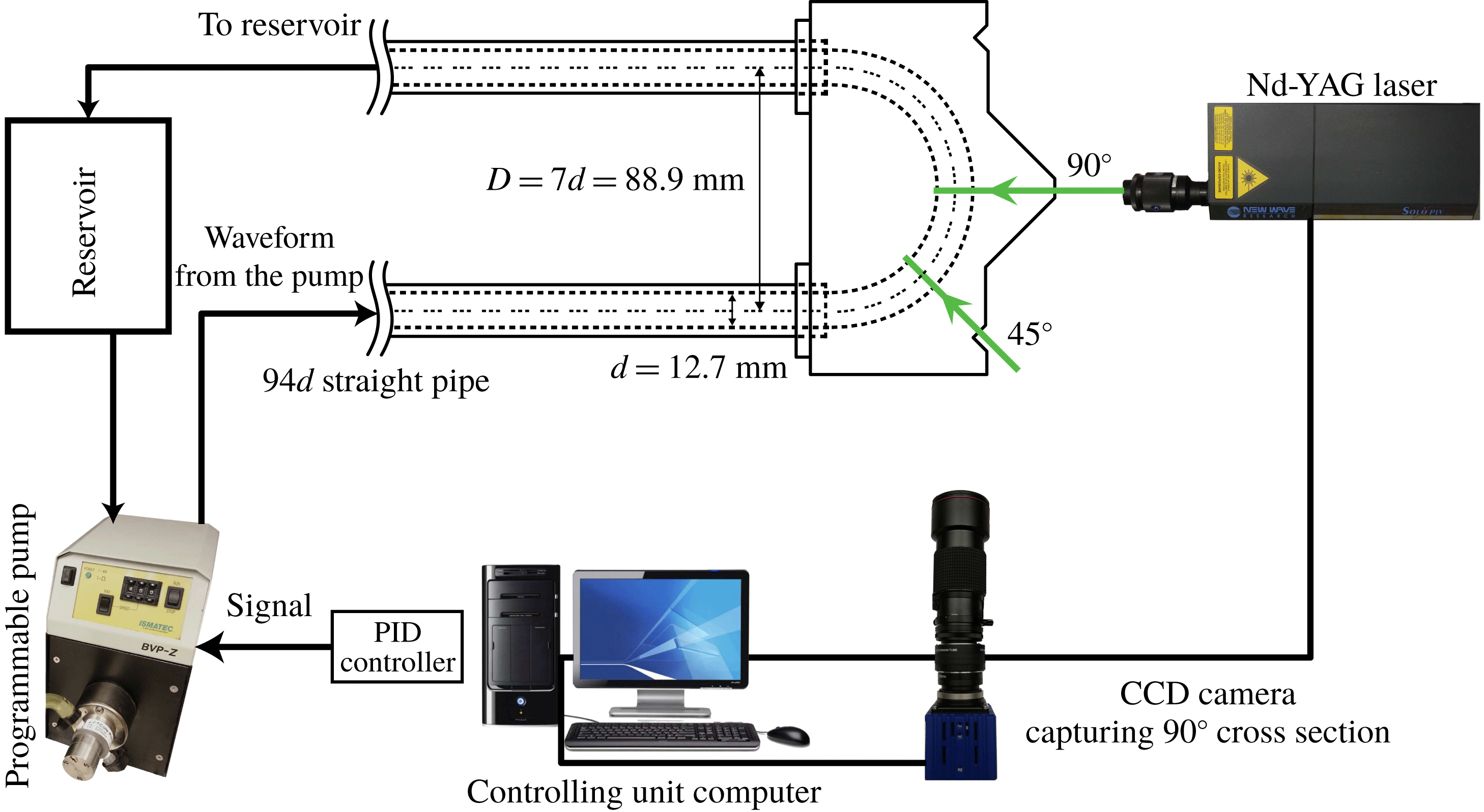
along the curve. Schematics of the test section, laser sheet locations and camera directions are shown in figure 1.
2.2 Inflow conditions
A
 $94d$
length of straight pipe was attached to the curve inlet to minimize upstream effects and disturbances at the curved test section (
 $d=12.7~\text{mm}$
). Although the flow upstream of the curved section is fully developed (axially invariant), the flow inside the curve is developing. The inflow waveforms were produced by a gear pump (Ismatec model BVP-Z). Once the desired input voltage to the pump is obtained using the PID (proportional–integral–derivative) controller (Najjari & Plesniak Reference Najjari and Plesniak2017), the pump and PIV system are controlled by a customized LabView program and a USB data acquisition device (NI USB-6229).
Schematic of experimental set-up, including test section, laser sheet location and camera direction.

2.3 Working fluid
The working fluid was a composition of water, glycerin and sodium iodide. The viscosity of the solution was set by the glycerin/water ratio, and the concentration of sodium iodide was varied to match the refractive index (RI) of the test section (sodium iodide concentration linearly increases the RI of glycerin–water mixture). Another advantage of adding sodium iodide to the solution is that it can prevent mould formation in the solution over time. Owing to oxidization of sodium iodide, the solution colour gradually changes over time, first to light yellow and then to red. Mixing approximately 0.5 g of sodium thiosulfate in 1 litre of the solution will restore the colour and make the fluid transparent again. It is found that the fluid with RI of 1.487 (measured by PAL-RI, Atago) matched the RI of our acrylic test sections perfectly.
The dynamic viscosity of the fluid was measured using a Discovery HR-2 (TA Instruments) rheometer with cone (
 $1^{\circ }:00^{\prime }:11^{\prime \prime }$
and 40 mm diameter) and flat-plate geometry with
 $24~\unicode[STIX]{x03BC}\text{m}$
gap under steady shear for three times, and the results were averaged. The dynamic viscosity
 $\unicode[STIX]{x1D707}$
was found to be
 $\unicode[STIX]{x1D707}=6\times 10^{-3}\pm 0.3\,\%~\text{Pa}~\text{s}$
. The density of the fluid was measured and was equal to
 $\unicode[STIX]{x1D70C}=1713\pm 1.1\,\%~\text{kg}~\text{m}^{-3}$
, producing a kinematic viscosity of
 $\unicode[STIX]{x1D708}=\unicode[STIX]{x1D707}/\unicode[STIX]{x1D70C}=3.5\times 10^{-6}~\text{m}^{2}~\text{s}^{-1}$
.
2.4 Particle image velocimetry (PIV)
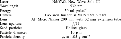
Phase-locked instantaneous velocity fields were measured using PIV. At each phase, 100 image pairs were acquired, which was shown to be sufficient for convergence (Najjari & Plesniak Reference Najjari and Plesniak2016). The PIV parameters are tabulated in table 1. DaVis 8 (LaVision) was used for the data acquisition and image post-processing.
PIV recording parameters.

For calibrating the PIV system, a custom-designed dotted map (with dot diameter of 0.5 mm and spacing of 1 mm) was created and printed on a transparency sheet. The printed map was then secured on a plastic fibre, allowing us to control the location of the calibration target accurately inside the test section. After the calibration target was placed inside the test section, the test section was filled with RI-matched fluid.
In the image post-processing step, the averaged background image was first subtracted, geometrical masking was then applied to the images, followed by the vector field calculation. A multi-pass option with decreasing window size from 64 pixels to 16 pixels with 50 % overlap was used for the interrogation area. This resulted in
 ${\approx}0.10~\text{mm}$
vector spacing and
 ${\approx}0.20~\text{mm}$
spatial resolution. In the final vector post-processing step, the vector allowable range, cross-correlation peak ratio criteria, median filter and
 $3\times 3$
smoothing are applied to the vector field.
The instantaneous velocity fields provided by DaVis software were input to an in-house Fortran code, which was used for further post-processing. In-plane spatial derivatives were calculated within the code using the second-order central finite difference method.
3 Transient flow rates
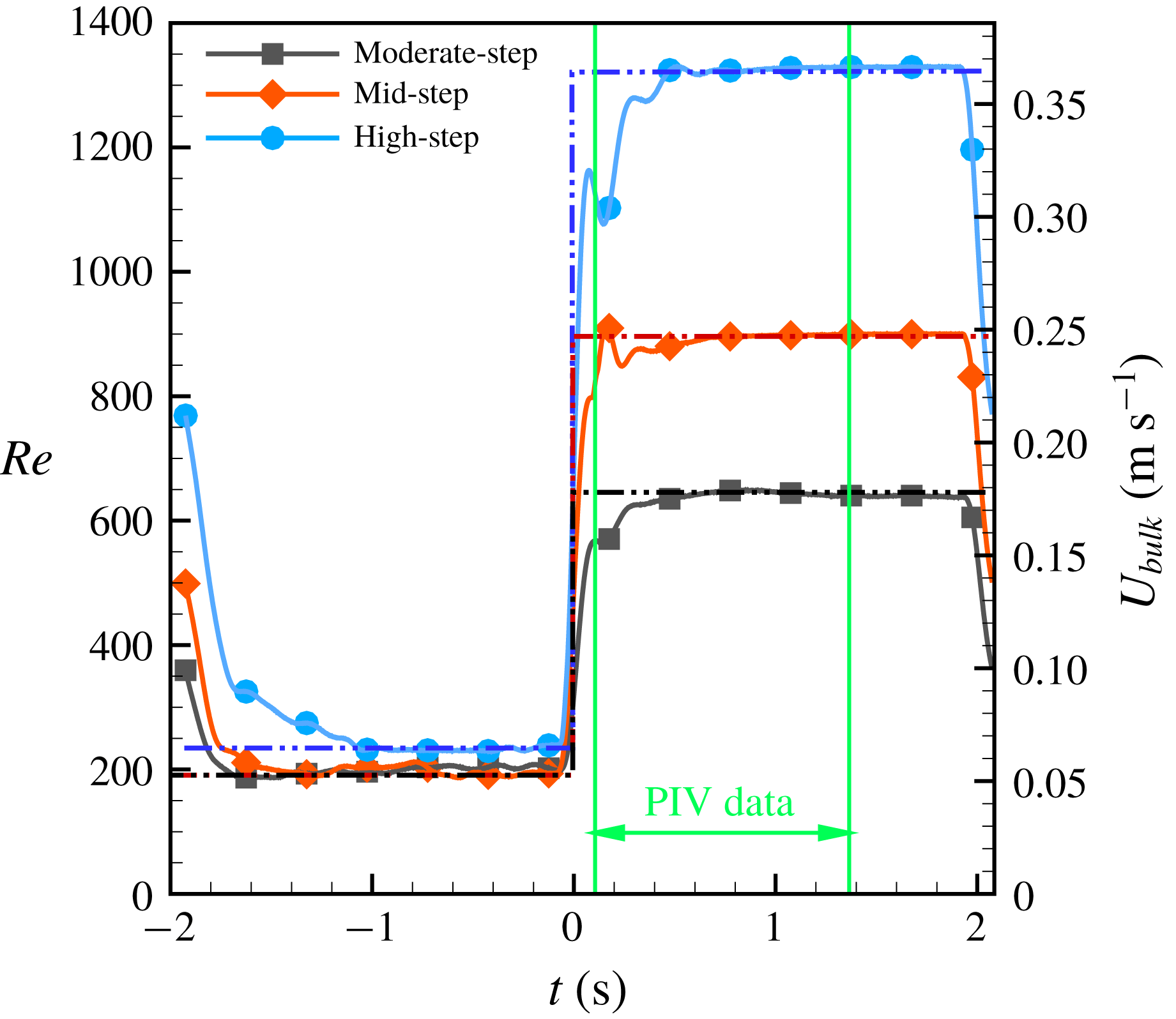
In order to investigate the formation and interaction of vortices in the curved pipe, three transient step-like flow rates are produced to allow study of the formation of different vortical structures. Figure 2 shows the three flow rates measured downstream of the test section by an ultrasonic flowmeter (Transonic ME12PXL), and table 2 lists the inflow details for these transient flow rates. The flow rates are well approximated by the shape of the mathematical Heaviside step function, and hence we employ the terminology ‘step flow’ to describe these transient flows. Because the experimental data acquisition requires multiple realizations per phase, the experimental flow rates are periodic in time. It was found that having low flow rate for
 ${\approx}1.5~\text{s}$
was sufficiently long to allow vortices from the previous cycle to decay and not interact with vortices that are being generated in the new cycle. Thus, for the experimental measurements the initial condition is
 ${\approx}1.5~\text{s}$
at low flow rates mentioned in table 2, and for CFD simulations the initial conditions are steady-state results. The negative time in figure 2, therefore, refers to the initial condition. Owing to the limitations of our pumping system, the experimental flows were not ideal and they did not have sharp edges. The flow rates oscillate before reaching their ideal high-flow-rate conditions mainly because of the internal built-in controller of the pump.
Three transient impulsively started, step-like flow rates. Solid lines are from experimental measurements and dashed–double dotted lines correspond to the ideal flow rates used in CFD simulations.

Details of the three flow rates investigated in this study.

4 Numerical solver
Since the experimental data are limited to the planar information without 3-D illustrations, simulations were performed to provide 3-D spatiotemporal data. ANSYS Fluent Academic Research Mechanical and CFD Release 19 (ANSYS Inc., Canonsburg, PA, USA) was used to perform simulations using steady and transient pressure-based viscous laminar flow solvers. In this paper steady-state results are obtained from a steady flow solver that provides physical results at steady state where the transient physics are not considered. Transient flow results are obtained using a special transient solver. For sufficiently long physical time (between 1.5 and 2 s) the transient solution converges to the steady-state solution. The geometry was designed in ANSYS Geometry Modular and meshing was performed by ANSYS meshing tool.
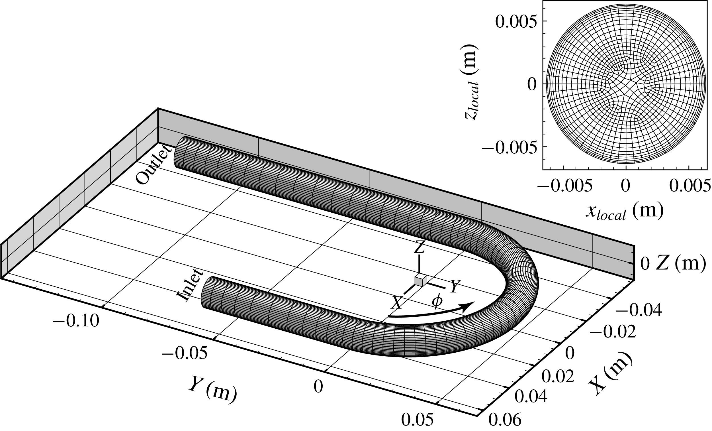
Three-dimensional view of the flow domain with a coarse mesh showing universal
 $X$
,
 $Y$
and
 $Z$
coordinates. The cross-sectional plane location is shown by
 $\unicode[STIX]{x1D719}$
, which is
 $0^{\circ }$
at the inlet and
 $180^{\circ }$
at the outlet. A cross-section of the pipe is also shown with local coordinates (
 $x_{local},z_{local}$
) defined in (4.1).

Fluent was only used for obtaining the solution and velocity gradients, with results post-processed by either Tecplot® or PyTecplot scripting. Figure 3 shows the coarse mesh of the
 $180^{\circ }$
geometry and orientation of the
 $X$
,
 $Y$
and
 $Z$
directions. The cross-sectional coordinate system is shown by
 $-r\leqslant x_{local}\leqslant r$
and
 $-r\leqslant z_{local}\leqslant r$
defined in (4.1), where
 $r=6.35~\text{mm}$
is the radius of the pipe and
 $D=88.9~\text{mm}$
is the diameter of the curvature:
 $$\begin{eqnarray}\left.\begin{array}{@{}c@{}}\displaystyle x_{local}=\sqrt{X^{2}+Y^{2}}-D/2,\quad 0^{\circ }\leqslant \unicode[STIX]{x1D719}\leqslant 180^{\circ },\\ \displaystyle z_{local}=Z.\end{array}\right\}\end{eqnarray}$$
The in-plane velocity magnitude
 $V$
refers to the secondary velocity magnitude at the cross-section, and
 $u$
,
 $v$
and
 $w$
are velocity components in
 $X$
,
 $Y$
and
 $Z$
directions, respectively. The axial (streamwise) velocity component which is normal to any cross-section is denoted by
 $V_{n}$
. All reported quantities such as velocity and vorticity are dimensional with SI units.
4.1 Boundary conditions
The simulations require inlet, outlet and wall boundary conditions. The inlet velocity profiles are defined at the inlet and a pressure outlet was used for the outlet. At the wall, either no-slip or slip conditions are enforced. A parabolic inlet velocity profile was used for steady-state flow simulations; inlet velocity profiles calculated analytically using the method in appendix B were used for transient flow simulations. After expressions for the inlet velocity profiles were obtained analytically, a user-defined-function (UDF) was written to introduce the correct inlet velocity profile at each physical time step for transient simulations. For these transient flows, the physical time step was set to
 $\unicode[STIX]{x0394}t=0.0005~\text{s}$
to satisfy the Courant–Friedrichs–Lewy (CFL) condition and guarantee convergence. The constructed geometry had a
 $5d$
straight inlet pipe upstream of the curve and a
 $10d$
straight pipe downstream of the curve to allow flow to develop and eliminate any upstream effect of the pressure outlet boundary condition.
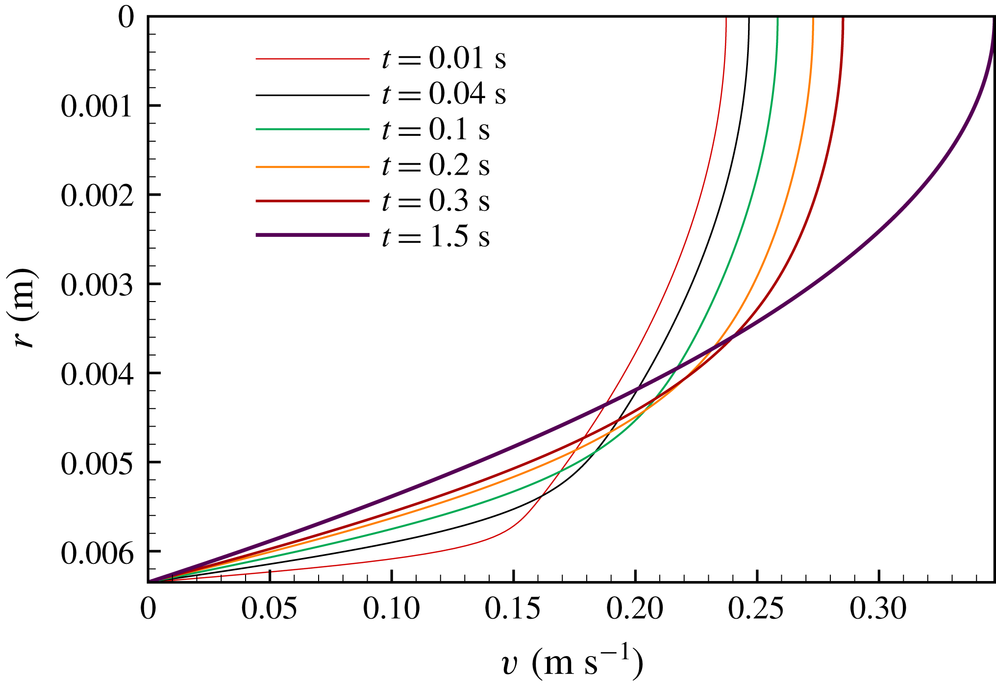
Figure 4 shows analytical velocity profiles obtained by the method provided in appendix B. These profiles are similar to a plug profile at the beginning of impulsive flows, and as time passes the profile converges to the parabolic shape inherent in Poiseuille flow.
Evolution of velocity profiles during the transient moderate-step flow rate at the inlet boundary condition obtained from analytical solution (appendix B). At
 $t=1.5~\text{s}$
, the flow has already reached the steady-state condition and the velocity profile has converged to a parabolic Poiseuille solution.

4.2 Grid independence
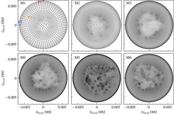
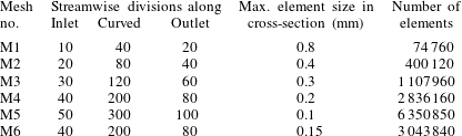
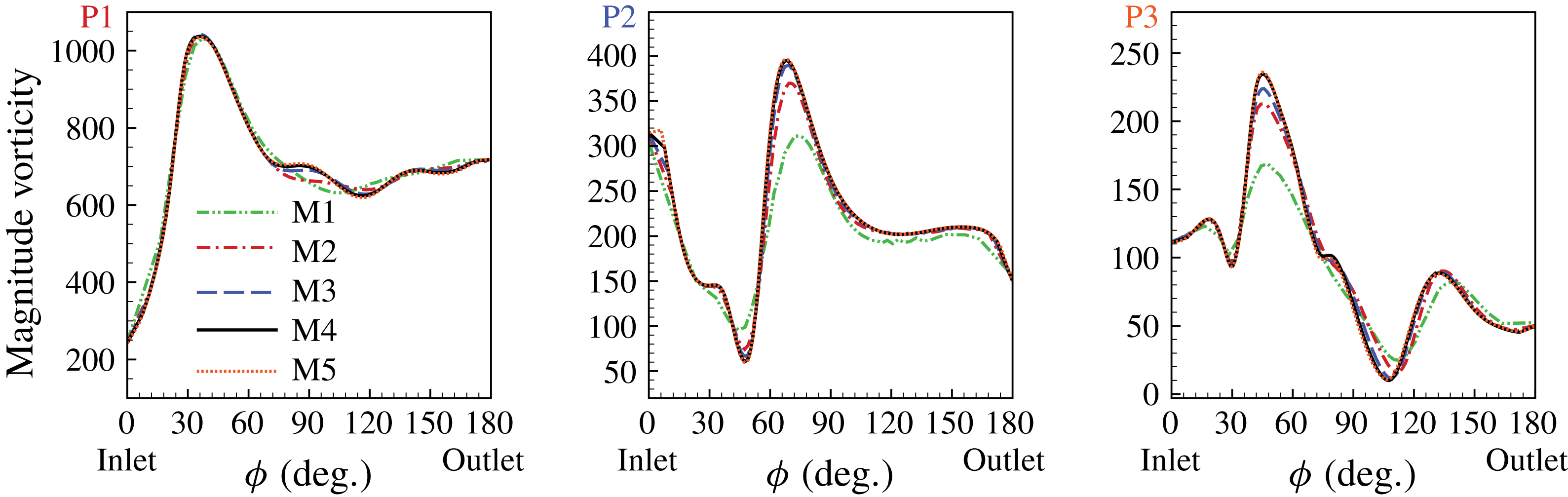
To obtain mesh-independent results, five different meshes (M1–M5, table 3) were generated for mesh convergence studies and the same simulations were performed using each one. Table 3 summarizes the parameters of each mesh and figure 5 shows the various mesh cross-sections. Meshes M1 and M5 are the coarsest and the finest mesh, respectively. Vorticity magnitude was computed for different meshes and tracked at several points inside the pipe. Figure 6 shows the vorticity magnitude at points P1–P3 (shown in figure 5) for five meshes. Refining the mesh from M4 to M5 does not change these results and, therefore, we conclude that converged results are achieved on the M4 mesh. However, since the elements near the core of the pipe in M4 are rather non-uniform in size, with rapid transition from small elements to larger ones, mesh M6 was generated to contain finer elements than M4 near the pipe core but coarser than M5. Ultimately, mesh M6 contains 3 043 840 elements and was used for all simulations.
Six different meshes shown at the cross-section of the pipe. Meshes M1 and M5 are the coarsest and the finest mesh, respectively. Mesh M6 is finer than M4 but coarser than M5, and this mesh is used for the simulations presented herein. The convergence of vorticity magnitude at points P1–P3 is shown in figure 6.

Details of meshes M1–M5 that were used for the mesh convergence study. Mesh M6, which is finer than M4 in the cross-section, was used to run the final simulations.

Vorticity magnitude along the streamwise direction at points P1–P3 shown in figure 5 for meshes M1–M5.

Comparison of in-plane velocity magnitude (
 $V$
) from experimental PIV results (a) and CFD results (b) at three time instants (
 $t=0.105$
, 0.525 and 1.365 s) for mid-step flow, at the
 $90^{\circ }$
cross-section of the curve. The experimental and simulation results match well with the correlation coefficient (4.2) of
 $c=97.9\,\%$
, 98.4 % and 97.4 % for
 $t=0.105$
, 0.525 and 1.365 s, respectively. The distribution of differences (c) between experimental and numerical in-plane velocity magnitude
 $V_{exp}(i,j)-V_{cfd}(i,j)$
.

4.3 CFD validation
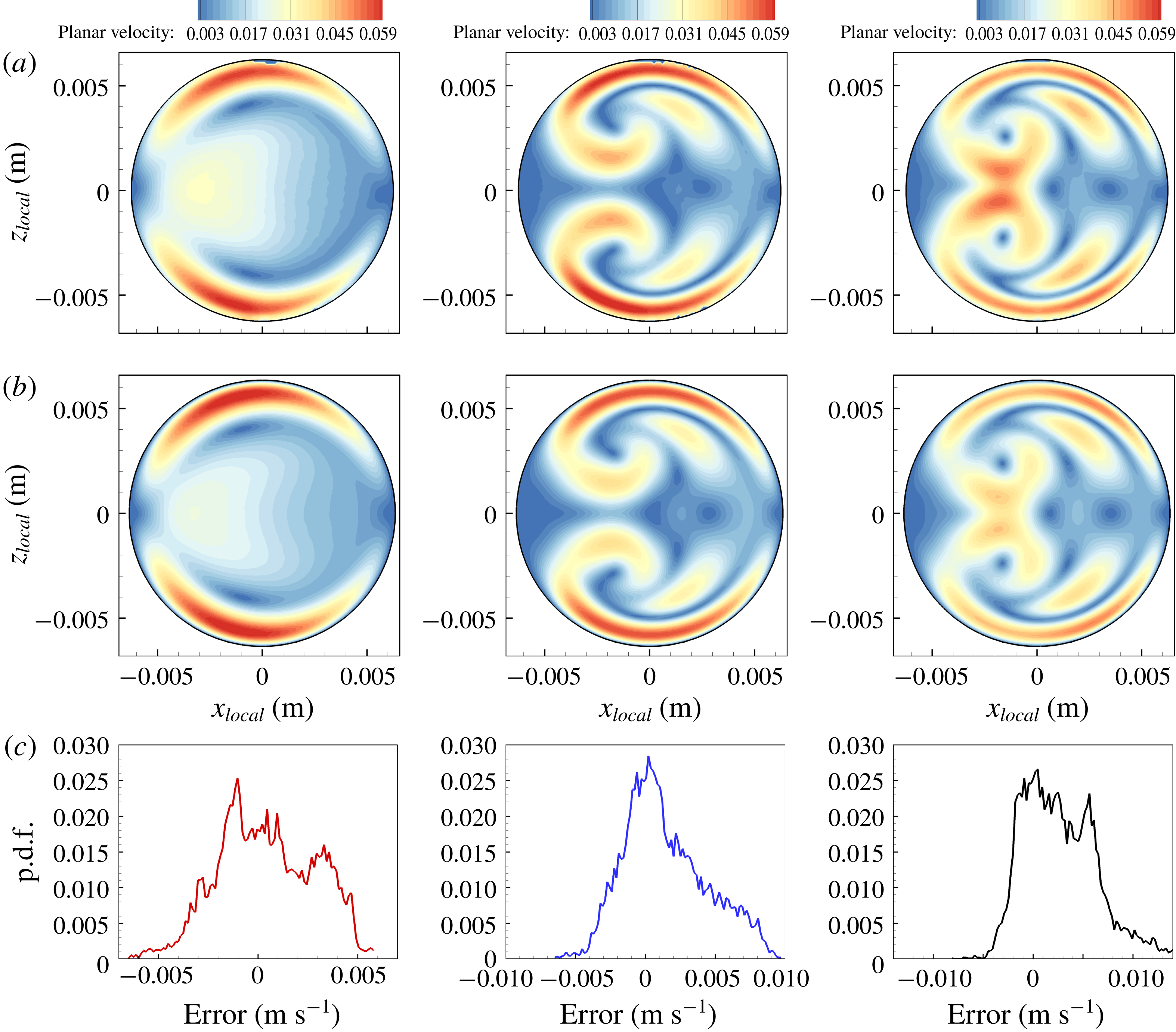
The in-plane velocity and vorticity results of our simulations are validated by the experimental results to benchmark the numerical simulations. To perform the comparisons, numerical data are transferred to a structured Cartesian mesh that exactly resembles the experimental PIV data mesh. The side-by-side comparisons of in-plane velocity maps are provided in figure 7, as well as the probability density function (p.d.f.) of error (
 $e_{ij}=V_{exp}(i,j)-V_{cfd}(i,j)$
), which is a point-by-point difference of the in-plane velocity magnitude of experimental and CFD results. Figure 7 shows the in-plane velocity magnitude at the
 $90^{\circ }$
cross-section for the transient mid-step flow rate at three phases. Excellent agreement between the PIV and CFD results was obtained. The spatial correlation between the numerical and experimental results is also calculated for both velocity and vorticity maps over time using 2-D Pearson’s correlation given in (4.2), where the overbar refers to spatial average:
 $$\begin{eqnarray}c=\frac{\displaystyle \mathop{\sum }_{i}\mathop{\sum }_{j}(V_{exp}(i,j)-\overline{V}_{exp})\times (V_{cfd}(i,j)-\overline{V}_{cfd})}{\sqrt{\displaystyle \mathop{\sum }_{i}\mathop{\sum }_{j}(V_{exp}(i,j)-\overline{V}_{exp})^{2}}\sqrt{\displaystyle \mathop{\sum }_{i}\mathop{\sum }_{j}(V_{cfd}(i,j)-\overline{V}_{cfd})^{2}}}.\end{eqnarray}$$
The calculated correlations for velocity are 97.9 %, 98.4 % and 97.4 % for
 $t=0.105$
, 0.525 and 1.365 s, respectively, further validating our results. Moreover, the p.d.f. of error shown in figure 7 demonstrates sufficiently low error.
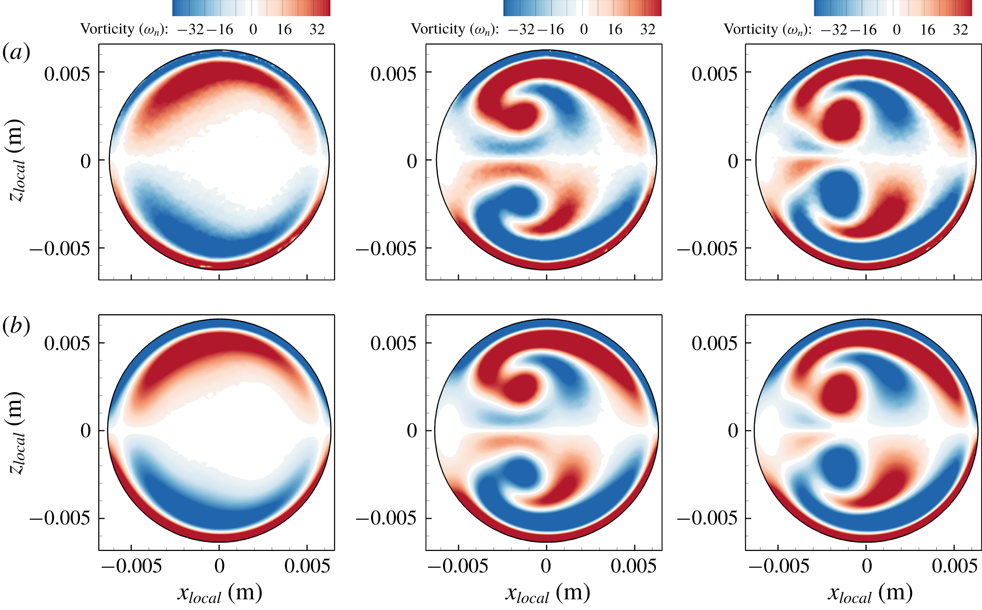
Comparison of vorticity results at different instants in time for mid-step flow rate from PIV and CFD data is shown in figure 8, which again shows an excellent match. The correlations between experimental and numerical streamwise vorticity fields are
 $c=97\,\%$
, 98.1 % and 98 % for
 $t=0.105$
, 0.525 and 1.365 s, respectively, which show a sufficiently high correlation.
Comparison of streamwise vorticity component from experimental PIV results (a) and CFD results (b) at three instants in time (
 $t=0.105$
, 0.525 and 1.365 s) for mid-step flow, at the
 $90^{\circ }$
cross-section of the curve. Small magnitudes of streamwise vorticity (
 $|\unicode[STIX]{x1D714}_{n}|<3.2~\text{s}^{-1}$
) are shown by white colour to delineate positive and negative regions. The experimental and simulation results agree with each other, with a correlation coefficient (4.2) of
 $c=97\,\%$
, 98.1 % and 98 % for
 $t=0.105$
, 0.525 and 1.365 s, respectively.

5 Vortex identification
To study the morphology of vortical structures, it is necessary to use legitimate vortex ID methods to distinguish vortical structures (swirling motions) from pure shear. Three Galilean-invariant methods for vortex ID are applied for 2-D and 3-D data. Once regions associated with proper vortices were identified, individual distinct vortical structures were identified in the cross-section to facilitate analysing each vortex separately. To obtain the vortex formation time, the circulation (
 $\unicode[STIX]{x1D6E4}$
) for each vortex in the cross-section of the pipe was calculated from (5.1) (see figure 24):
 $$\begin{eqnarray}\unicode[STIX]{x1D6E4}=\oint _{r}\boldsymbol{u}\boldsymbol{\cdot }\text{d}\boldsymbol{r}=\int _{\boldsymbol{s}}\unicode[STIX]{x1D74E}\boldsymbol{\cdot }\boldsymbol{n}\,\text{d}\boldsymbol{s}=\unicode[STIX]{x0394}x_{local}\unicode[STIX]{x0394}z_{local}\mathop{\sum }_{vortex\;area}\unicode[STIX]{x1D714}_{n},\end{eqnarray}$$
where
 $\unicode[STIX]{x1D74E}\boldsymbol{\cdot }\boldsymbol{n}=\unicode[STIX]{x1D714}_{n}$
refers to the streamwise component of vorticity (normal to pipe cross-sections) with the summation being performed over the area occupied by each vortex.
5.1 Two-dimensional vortex ID
The
 $d_{2}$
method (discriminant of non-real eigenvalues of velocity gradient matrix (Vollmers Reference Vollmers2001)) defined in (5.2) is a Galilean-invariant method used to identify the vortical structures in the secondary flow using 2-D data:
 $$\begin{eqnarray}d_{2}=\left(\frac{\unicode[STIX]{x2202}u_{x_{local}}}{\unicode[STIX]{x2202}x_{local}}+\frac{\unicode[STIX]{x2202}w}{\unicode[STIX]{x2202}Z}\right)^{2}-4\left(\frac{\unicode[STIX]{x2202}u_{x_{local}}}{\unicode[STIX]{x2202}x_{local}}\frac{\unicode[STIX]{x2202}w}{\unicode[STIX]{x2202}Z}-\frac{\unicode[STIX]{x2202}u_{x_{local}}}{\unicode[STIX]{x2202}Z}\frac{\unicode[STIX]{x2202}w}{\unicode[STIX]{x2202}x_{local}}\right).\end{eqnarray}$$
This method is based on the swirling strength criterion (Zhou et al.
Reference Zhou, Adrian, Balachandar and Kendall1999) definition. A negative value of
 $d_{2}$
indicates a vortex region. Since
 $d_{2}$
can only be applied to 2-D data, if local coordinates were not aligned with the main coordinate axes (e.g.
 $45^{\circ }$
cross-section), a directional derivative formulation was used to calculate
 $d_{2}$
.
5.2 Three-dimensional vortex ID
In order to identify vortices in 3-D data, several methods such as
 $Q$
-criterion (Hunt, Wray & Moin Reference Hunt, Wray and Moin1988), swirling strength criterion (Zhou et al.
Reference Zhou, Adrian, Balachandar and Kendall1999) and
 $\unicode[STIX]{x1D706}_{2}$
criterion (Jeong & Hussain Reference Jeong and Hussain1995) are available. For a detailed review on different vortex ID methods, see Chakraborty, Balachandar & Adrian (Reference Chakraborty, Balachandar and Adrian2005). In this study we used
 $\unicode[STIX]{x1D706}_{2}$
and swirling strength criteria for identifying vortices in three dimensions.
5.2.1 The
$\unicode[STIX]{x1D706}_{2}$
criterion

The
 $\unicode[STIX]{x1D706}_{2}$
criterion identifies a vortex region if the middle eigenvalue of the matrix
 $\unicode[STIX]{x1D734}^{2}+\unicode[STIX]{x1D64E}^{2}$
is negative (
 $\unicode[STIX]{x1D706}_{2}<0$
), where
 $\unicode[STIX]{x1D64E}={\textstyle \frac{1}{2}}(\unicode[STIX]{x1D735}\unicode[STIX]{x1D66A}+(\unicode[STIX]{x1D735}\unicode[STIX]{x1D66A})^{\text{t}})$
is the symmetric component of the velocity gradient tensor (
 $\unicode[STIX]{x1D735}\unicode[STIX]{x1D66A}$
), and
 $\unicode[STIX]{x1D734}={\textstyle \frac{1}{2}}(\unicode[STIX]{x1D735}\unicode[STIX]{x1D66A}-(\unicode[STIX]{x1D735}\unicode[STIX]{x1D66A})^{\text{t}})$
is the antisymmetric part of
 $\unicode[STIX]{x1D735}\unicode[STIX]{x1D66A}$
. If
 $\unicode[STIX]{x1D706}_{1}\geqslant \unicode[STIX]{x1D706}_{2}\geqslant \unicode[STIX]{x1D706}_{3}$
are the eigenvalues of the matrix
 $\unicode[STIX]{x1D734}^{2}+\unicode[STIX]{x1D64E}^{2}$
, then regions of negative
 $\unicode[STIX]{x1D706}_{2}$
indicate vortex regions. The velocity gradients are directly exported from the solver (§ 4) to Tecplot for post-processing and calculation of
 $\unicode[STIX]{x1D706}_{2}$
. Since
 $\unicode[STIX]{x1D734}^{2}+\unicode[STIX]{x1D64E}^{2}$
is a symmetric matrix, the eigenvalues of
 $\unicode[STIX]{x1D734}^{2}+\unicode[STIX]{x1D64E}^{2}$
are real, so they are calculated analytically using the trigonometric solution for the roots of a cubic equation to verify the numerical approach for calculating eigenvalues of
 $\unicode[STIX]{x1D734}^{2}+\unicode[STIX]{x1D64E}^{2}$
. An excellent match was obtained between analytical and numerical methods, and hence the numerical method was preferred for its simplicity and lower processing time.
5.2.2 Swirling strength criterion
The ‘swirling strength’ criterion introduced by Zhou et al. (Reference Zhou, Adrian, Balachandar and Kendall1999) detects vortices when the velocity gradient tensor (
 $\unicode[STIX]{x1D735}\unicode[STIX]{x1D66A}$
) has complex eigenvalues of (
 $\unicode[STIX]{x1D706}_{cr}\pm \text{i}\unicode[STIX]{x1D706}_{ci}$
) and a real eigenvalue (
 $\unicode[STIX]{x1D706}_{r}$
) at a given point. The
 $\unicode[STIX]{x1D706}_{ci}$
value is positive and its magnitude is an indication of the vortex strength. Another useful feature of the swirling strength method is that by calculating the eigenvectors associated with complex eigenvalues (i.e.
 $\unicode[STIX]{x1D742}_{cr}\pm \text{i}\unicode[STIX]{x1D742}_{ci}$
) the orientation of the vortex axis can be found because the plane spanned by vectors
 $\unicode[STIX]{x1D742}_{cr}$
and
 $\unicode[STIX]{x1D742}_{ci}$
is the plane of rotation (Zhou et al.
Reference Zhou, Adrian, Balachandar and Kendall1999; Chakraborty et al.
Reference Chakraborty, Balachandar and Adrian2005) – figure 20 shows the results of this analysis.
To calculate the complex eigenvalues of
 $\unicode[STIX]{x1D735}\unicode[STIX]{x1D66A}$
, the velocity gradients were directly output from the Fluent solver into Tecplot format and post-processed using a custom PyTecplot script.
6 Results and discussion
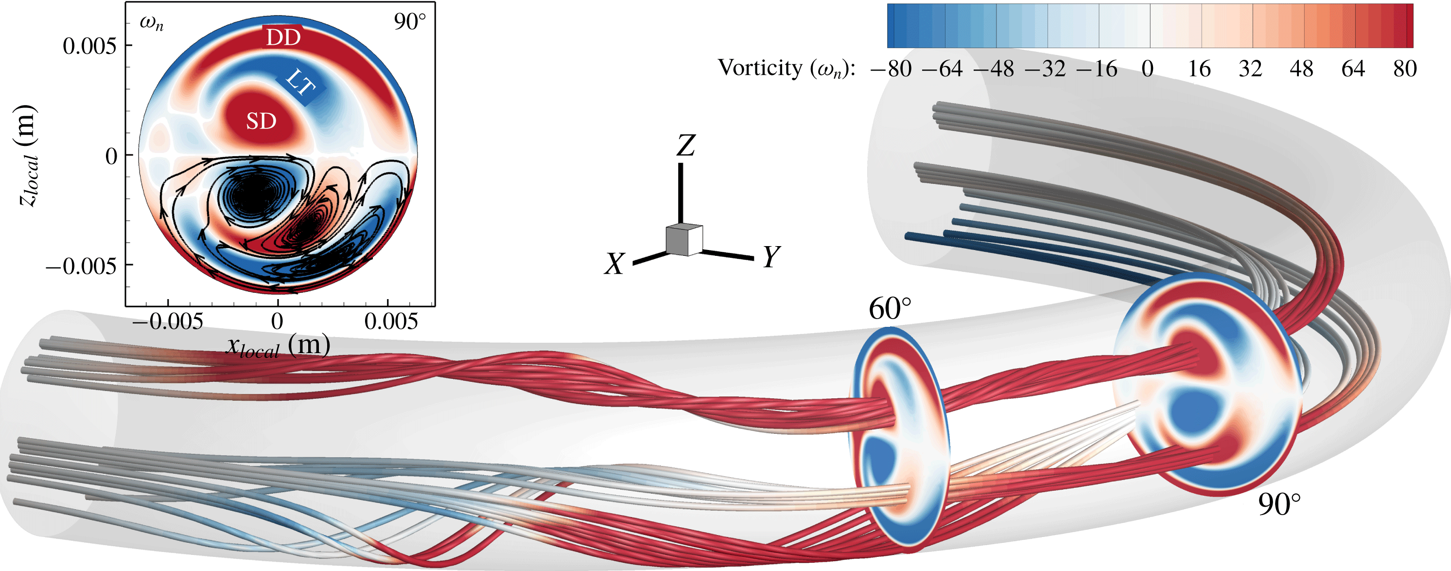
The main features of the flow are shown in terms of vorticity and streamlines inside the curved pipe for high-step flow in figure 9. Vortices defined herein as deformed Dean (DD), split Dean (SD) and Lyne type (LT) are shown in the inset by the streamwise vorticity and 2-D streamlines. In figure 9 the 3-D streamlines in the split-Dean location are highly spiral and twisted, whereas streamlines in the Lyne-type vortex show weak spiral motion. To augment the streamlines and vorticity plots, several vortex ID methods are used to identify vortex core regions. Later in this section, the evolution of different vortical structures is determined by various methods and their results are compared.
Three-dimensional streamlines coloured by streamwise vorticity (
 $\unicode[STIX]{x1D714}_{n}$
) for high-step flow rate at
 $t=2.01~\text{s}$
. The inset shows the
 $90^{\circ }$
cross-section with 2-D streamlines (secondary flow) and a depiction of deformed-Dean (DD), split-Dean (SD) and Lyne-type (LT) vortices.

In this section, the evolution of the vorticity field is discussed first, followed by the vorticity transport equation analysis to identify the mechanism for formation of the Lyne-type vortex. These results include both the physical no-slip and (idealized) slip wall models in order to study the effect of wall vorticity on the formation of the Lyne-type vortex. It will be shown that the Lyne-type vortex is different from the classical Lyne vortex pair in oscillatory flows, but, due its visual similarities in the cross-sectional data to the classical Lyne vortex pair, we designate this vortex in steady, transient or pulsatile flows as a Lyne-type vortex. Later in this section, the differences between the classical Lyne vortex pair and the Lyne-type vortex will be discussed as well as the dynamics of the flow by investigating momentum balance and centrifugal force.
Since the main focus of the current paper is to characterize the Lyne-type vortex and distinguish it from the classical Lyne vortex pair, most of the results presented in this section are for the moderate-step flow, where the formation time of the Lyne-type vortex is greater than in the two other cases. With this longer formation time, transient features can be better analysed given the constant temporal resolution of
 $\unicode[STIX]{x0394}t=0.0005~\text{s}$
. Additionally, the split-Dean vortex pair depicted in figure 9 occurs for
 $Re>890$
in this geometry. Cox (Reference Cox2017) discussed mechanisms responsible for vortex splitting which are beyond the scope of the current study.
6.1 Evolution of vorticity
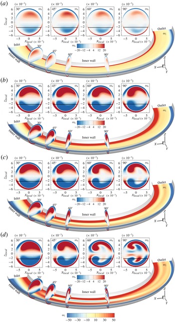
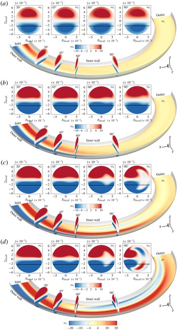
Figures 10 and 11 show the vorticity components normal to each plane for four instants in time under no-slip and slip wall conditions, respectively, for moderate-step flow rate. Supplemental movies 1 and 2 (available online at https://doi.org/10.1017/jfm.2019.510) also show these vorticity plots under these wall conditions, respectively. In figure 10, the vorticity component in the
 $Z$
direction (
 $\unicode[STIX]{x1D714}_{z}$
, shown in the axial slices) is strong and generated due to the no-slip wall, and is initially concentrated in the vicinity of the wall while the streamwise vorticity (
 $\unicode[STIX]{x1D714}_{n}$
) in the cross-sections is weak. As time passes,
 $\unicode[STIX]{x1D714}_{n}$
strengthens and
 $\unicode[STIX]{x1D714}_{z}$
is transported to the interior regions. During this transient flow, positive
 $\unicode[STIX]{x1D714}_{z}$
(at the inner wall) forms a branch away from the inner wall at
 $t=0.24~\text{s}$
around the
 $45^{\circ }$
cross-section for the no-slip condition (figures 10
b and 12). This branch grows in time and reaches the
 $90^{\circ }$
cross-section at
 $t=0.315~\text{s}$
(figures 10
c and 12). The branch of
 $\unicode[STIX]{x1D714}_{z}$
at the interior region coincides with the location of the Lyne-type vortex at the
 $90^{\circ }$
cross-section of the pipe shown by
 $\unicode[STIX]{x1D714}_{n}$
in figure 10(c,d). Later in this section, a vortex ID isosurface will confirm that this branch of
 $\unicode[STIX]{x1D714}_{z}$
is attributable to the Lyne-type vortex.
Vorticity component normal to each plane for moderate-step flow rate with no-slip wall condition at (a)
 $t=0.015~\text{s}$
, (b)
 $t=0.24~\text{s}$
, (c)
 $t=0.315~\text{s}$
and (d)
 $t=0.9~\text{s}$
. Four cross-sectional slices are shown at
 $30^{\circ }$
,
 $45^{\circ }$
,
 $60^{\circ }$
and
 $90^{\circ }$
locations, and the axial slice location is at
 $Z=-2.5~\text{mm}$
, indicated by the black line in the cross-sectional views. Vorticity component along the
 $Z$
direction (shown in axial slice) forms a branch at
 $t\approx 0.24~\text{s}$
between
 $30^{\circ }$
and
 $60^{\circ }$
near the inner wall. This vorticity region is connected to the Lyne-type vortex region later in time (see movie 1 for more phases).

Vorticity component normal to each plane for moderate-step flow rate with slip wall condition at (a)
 $t=0.48~\text{s}$
, (b)
 $t=0.66~\text{s}$
, (c)
 $t=0.9~\text{s}$
and (d)
 $t=1.2~\text{s}$
. Four cross-sectional slices are shown at
 $30^{\circ }$
,
 $45^{\circ }$
,
 $60^{\circ }$
and
 $90^{\circ }$
locations, and the axial slice location is at
 $Z=-2.5~\text{mm}$
, indicated by the black line in the cross-sectional views. Vorticity component along the
 $Z$
direction (shown in axial slice) which is introduced by inlet velocity profile propagates through the curved pipe and forms the Lyne-type vortex region later in time (see movie 2).

The slip wall model is investigated in order to determine whether the Lyne-type vortex is associated with the vorticity that is generated at the inner wall of the curved pipe or if it can form even without wall vorticity. For the slip wall model, figure 11, similar behaviour of vorticity is observed, with some differences. Firstly, due to the elimination of the wall contribution in the generation of vorticity, the overall vorticity level is lower than that under the no-slip wall condition. Additionally, since the vorticity is not produced at the wall, it is either convected into the curved section (i.e. vorticity introduced by the inlet velocity profile) or generated in the curved section. Figure 11(a–d) and movie 2 show that positive and negative
 $\unicode[STIX]{x1D714}_{z}$
propagate into the curve from the inlet of the curve as time passes, and this vorticity region is not connected to the wall near the inlet. Therefore, this vorticity is initially introduced in the flow by the physical velocity profile introduced at the inlet boundary and then transported to the curved section. Another major difference between the slip and no-slip wall results is the latency in the formation of Lyne-type vortex in the slip model. For instance, the Lyne-type vortex first appeared at the
 $90^{\circ }$
cross-section at
 $t\approx 0.315~\text{s}$
for the no-slip wall, and at
 $t\approx 0.78~\text{s}$
for the slip wall model. Therefore, although the vorticity generated at the wall increases the strength of Lyne-type vortex and accelerates its formation, the Lyne-type vortex can be generated without the wall vorticity present albeit with lower strength and slower in time.
Vorticity
 $Z$
component (
 $\unicode[STIX]{x1D714}_{z}$
) for the moderate-step flow rate with no-slip wall condition at (a)
 $t=0.015~\text{s}$
, (b)
 $t=0.21~\text{s}$
, (c)
 $t=0.24~\text{s}$
and (d)
 $t=0.315~\text{s}$
at the axial slice of
 $Z=-2.5~\text{mm}$
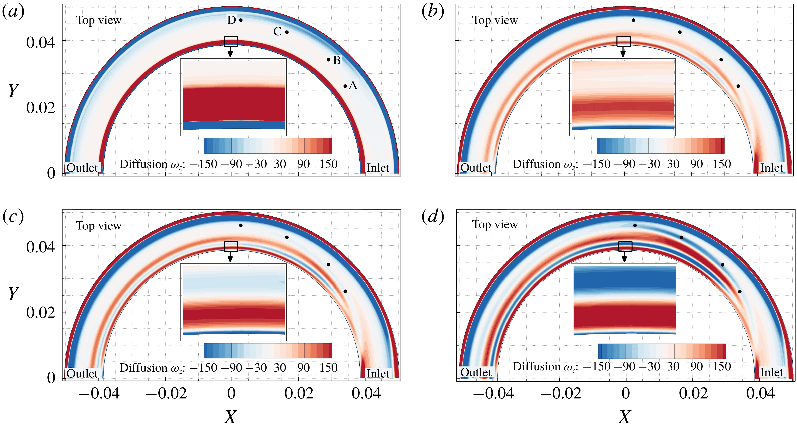
. Points A, B, C and D are placed at the location of the
 $\unicode[STIX]{x1D714}_{z}$
branch at
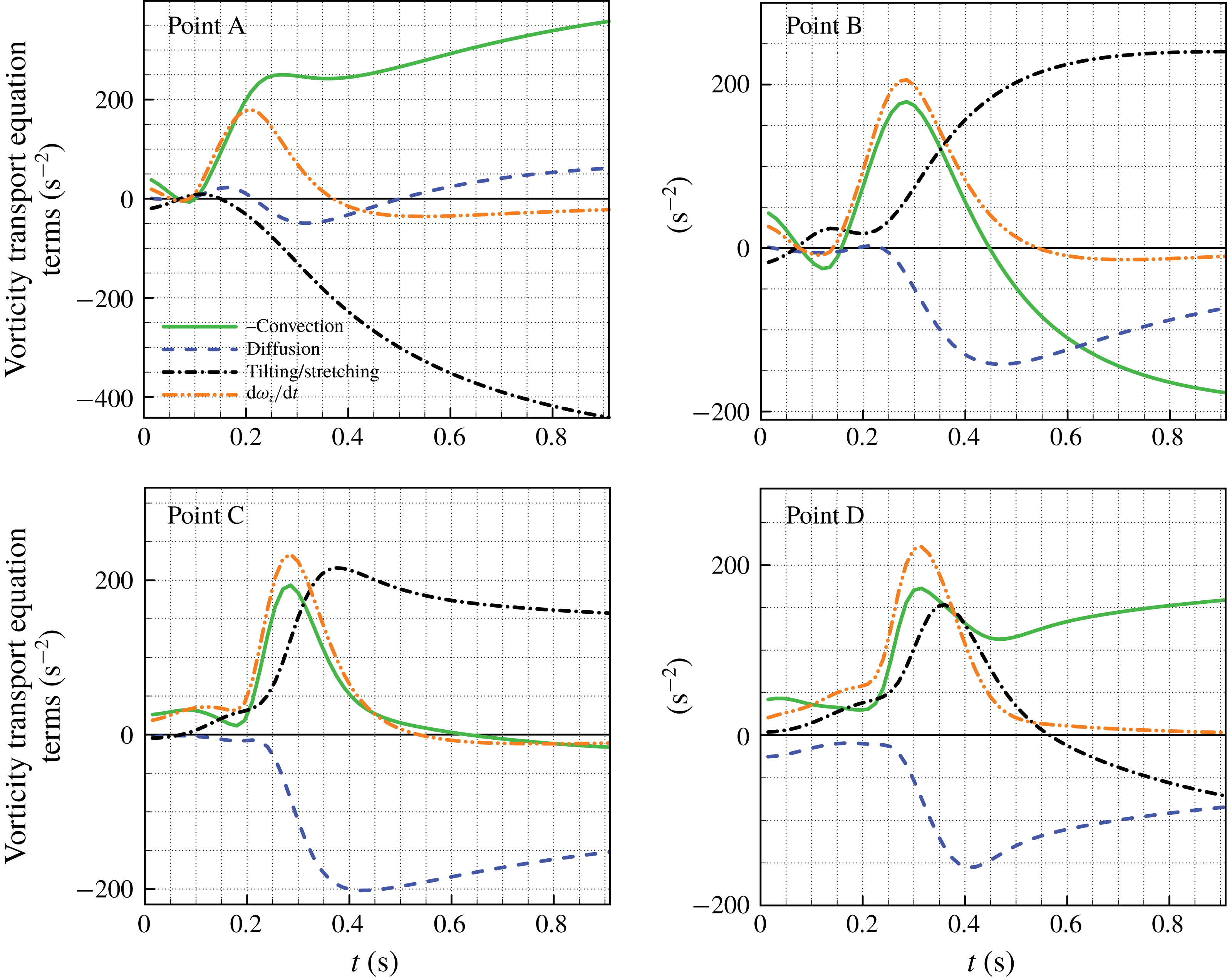
 $t\gtrsim 0.21~\text{s}$
, which corresponds to the location of the Lyne-type vortex. The balance of vorticity transport equation terms are shown at these four points in figure 16 to support our hypothesis of vorticity convection.

Spatiotemporal evolution of
 $\unicode[STIX]{x1D714}_{z}$
in the slip wall model shows that positive
 $\unicode[STIX]{x1D714}_{z}$
appears at the inner wall region near the entrance to the curve (it is convected from the inlet boundary). When this shear layer enters the curved section, it moves away from the inner wall due to wall curvature, and when the flow rate is high enough, this shear layer peels off because it cannot follow the wall curvature throughout the entire curve. This shear layer is then convected away from the wall to the interior of the flow. In this region
 $\unicode[STIX]{x1D714}_{z}$
contributes to the formation of the Lyne-type vortex. Similar flow physics occur in the no-slip wall model (figure 10), and because new vorticity is generated along the inner wall in this case,
 $\unicode[STIX]{x1D714}_{z}$
vorticity contours appear to branch off from the inner wall. Another mechanism that contributes to the branching of
 $\unicode[STIX]{x1D714}_{z}$
and transporting it to the interior region is the secondary flow induced by the Dean vortices which convects the vorticity from the wall region to the interior.
At the
 $90^{\circ }$
cross-section in figure 11(b), and
 $60^{\circ }$
cross-section in figure 11(c,d), the streamwise vorticity (which is part of the deformed-Dean vortex) is pushed away from the centreline of the pipe as the Lyne-type vortex forms. The Lyne-type vortex needs space in the cross-section of the pipe downstream of
 $\unicode[STIX]{x1D719}=30^{\circ }$
, which results in a decrease of the area of the deformed-Dean vortex. As the area of the deformed-Dean vortex is reduced, its circulation also declines over time when the Lyne-type vortex is forming (see figure 24).
6.1.1 Vorticity transport equation results, moderate-step flow
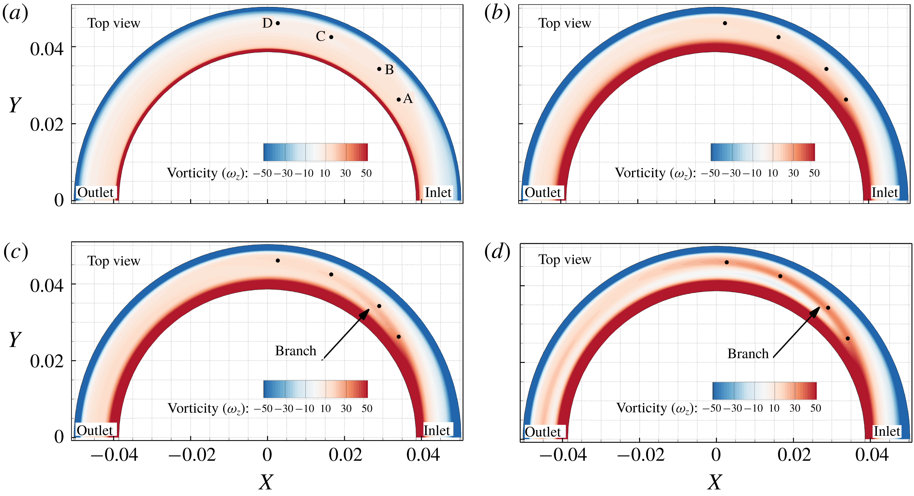
Figure 12 shows
 $\unicode[STIX]{x1D714}_{z}$
for moderate-step flow with a no-slip condition at four instants in time, where the branching from positive
 $\unicode[STIX]{x1D714}_{z}$
at the inner wall proximity is clear. This branch contributes to the formation of the Lyne-type vortex. Four points are placed at specific locations within this vorticity region, and the distributions of vorticity transport equation terms for these four points are shown in figure 16.
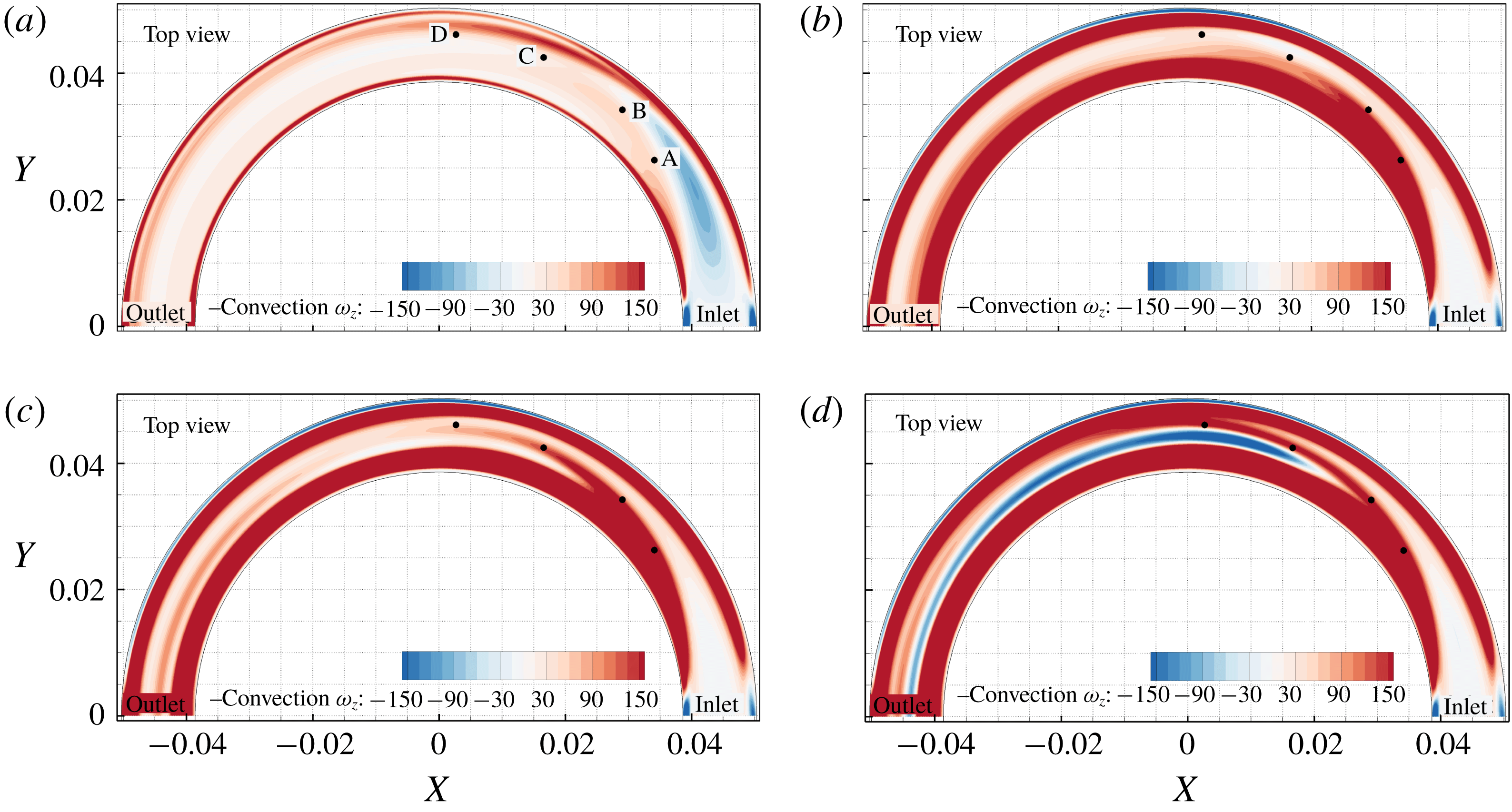
Figure 13 shows the negative convection term (to represent its value when moved to the right-hand side of (6.1)) for the same flow conditions as above. If we treat
 $\unicode[STIX]{x1D714}_{z}$
as a scalar, then we can describe its transport by the convection term. The convection term is zero at the wall because of the no-slip condition and peaks near the wall. The
 $\unicode[STIX]{x1D714}_{z}$
component of vorticity is being transported away from the wall first by viscous diffusion and afterwards by convection in the interior region. Therefore, convection peaks slightly away from the wall at
 $t=0.015~\text{s}$
. Figure 13 shows a branch forming in convection between points B and C at
 $t=0.21~\text{s}$
, while at this time the plot in figure 12 does not show the formation of the
 $\unicode[STIX]{x1D714}_{z}$
branch.
Negative convection of
 $\unicode[STIX]{x1D714}_{z}$
in (6.1) for the moderate-step flow rate with no-slip wall condition at (a)
 $t=0.015~\text{s}$
, (b)
 $t=0.21~\text{s}$
, (c)
 $t=0.24~\text{s}$
and (d)
 $t=0.315~\text{s}$
at the axial slice of
 $Z=-2.5~\text{mm}$
.

It is important to note that the diffusion of vorticity is occurring as a consequence of the diffusion of momentum via molecular interactions, which changes the velocity gradient (Morton Reference Morton1984):
 $$\begin{eqnarray}\frac{\unicode[STIX]{x2202}\unicode[STIX]{x1D714}_{z}}{\unicode[STIX]{x2202}t}+(\unicode[STIX]{x1D66A}\boldsymbol{\cdot }\unicode[STIX]{x1D735})\unicode[STIX]{x1D714}_{z}=(\unicode[STIX]{x1D74E}\boldsymbol{\cdot }\unicode[STIX]{x1D735})w+\unicode[STIX]{x1D708}\unicode[STIX]{x1D6FB}^{2}\unicode[STIX]{x1D714}_{z}.\end{eqnarray}$$
The tilting and stretching term (
 $(\unicode[STIX]{x1D74E}\boldsymbol{\cdot }\unicode[STIX]{x1D735})w$
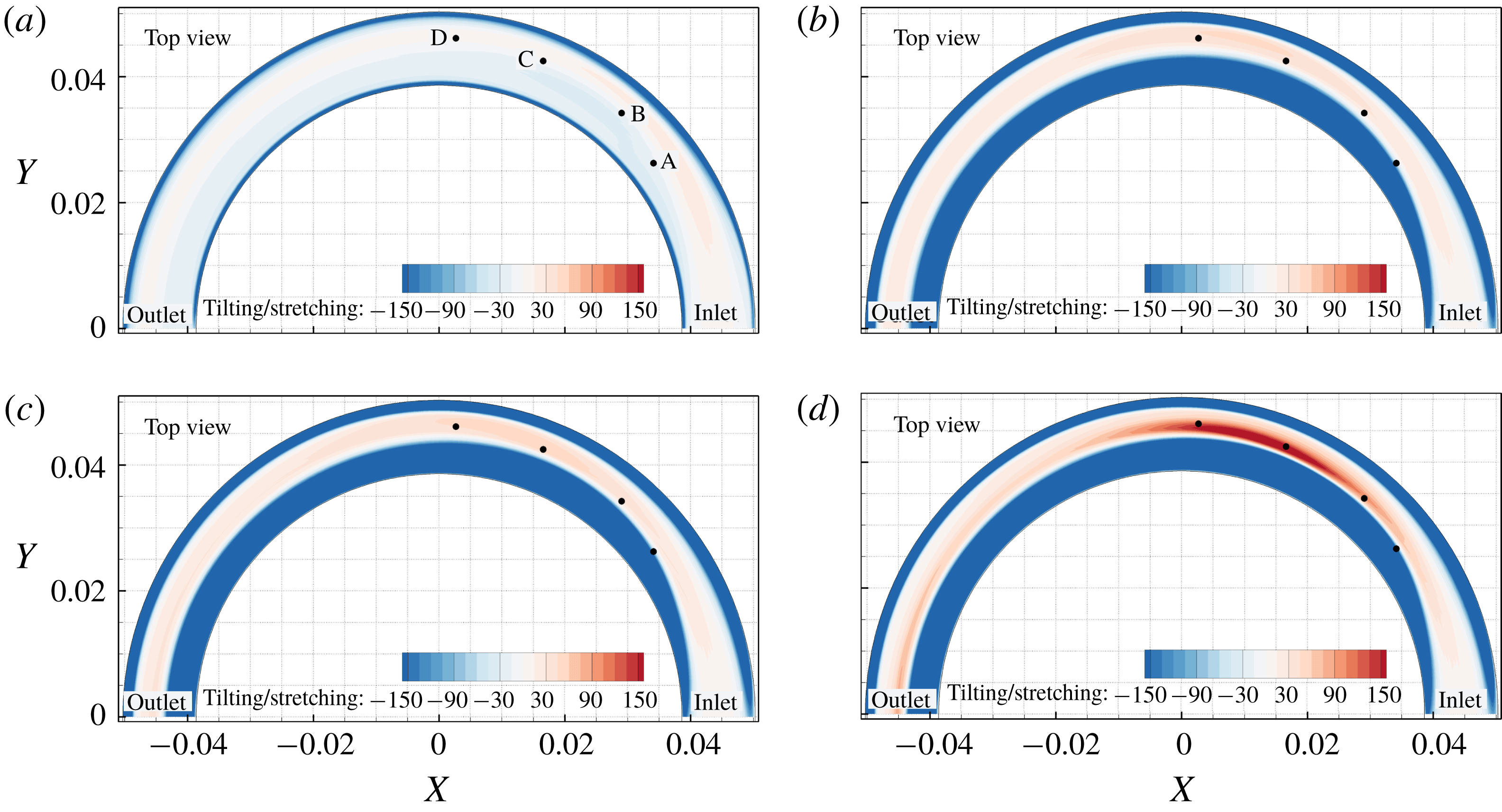
) in the vorticity transport equation is responsible for intensification/dilution of vorticity by the act of stretching/compression and rotation of the vorticity vector, which results in an increase in one component and corresponding decrease in (an)other component(s). Figure 14 shows this term for four instants in time at
 $Z=-2.5~\text{mm}$
. At this axial slice the tilting/stretching term is positive but has lower values than the convection term in the location of Lyne-type vortex during its formation phases (points A–D).
Tilting and stretching term in (6.1) for the moderate-step flow rate with no-slip wall condition at (a)
 $t=0.015~\text{s}$
, (b)
 $t=0.21~\text{s}$
, (c)
 $t=0.24~\text{s}$
and (d)
 $t=0.315~\text{s}$
at the axial slice of
 $Z=-2.5~\text{mm}$
.

The diffusion term (
 $\unicode[STIX]{x1D708}\unicode[STIX]{x1D6FB}^{2}\unicode[STIX]{x1D714}_{z}$
) in (6.1) is shown in figure 15 for the same flow conditions as in figure 12. It is clear that at
 $t=0.015~\text{s}$
the vorticity is concentrated in the wall region, and hence the diffusion is at its maximum at the wall. Figure 15 insets show zoomed views of the diffusion term where a negative narrow region of diffusion exists. Since
 $\unicode[STIX]{x1D714}_{z}$
is positive at the inner wall, the diffusion term is negative in this region, indicating that the vorticity generated because of the wall is being transported to the interior regions by the act of viscous diffusion of momentum. On the outer wall,
 $\unicode[STIX]{x1D714}_{z}$
is negative, and since the diffusion always reduces the extrema magnitude over time, the diffusion term is positive at this region, which counteracts the growth of
 $\unicode[STIX]{x1D714}_{z}$
by reducing the magnitude of
 $\unicode[STIX]{x2202}\unicode[STIX]{x1D714}_{z}/\unicode[STIX]{x2202}t$
. The contributions of vorticity transport terms to the changes in the vorticity field should be interpreted with respect to the sign of vorticity components locally.
Diffusion of
 $\unicode[STIX]{x1D714}_{z}$
in (6.1) for the moderate-step flow rate with no-slip wall condition at (a)
 $t=0.015~\text{s}$
, (b)
 $t=0.21~\text{s}$
, (c)
 $t=0.24~\text{s}$
and (d)
 $t=0.315~\text{s}$
at the axial slice of
 $Z=-2.5~\text{mm}$
. Insets show that the diffusion is high in close vicinity to the pipe wall at
 $t=0.015~\text{s}$
which transports
 $\unicode[STIX]{x1D714}_{z}$
into the interior region from the wall.

In order to evaluate the contribution of each term in the vorticity transport equation to the variations of
 $\unicode[STIX]{x1D714}_{z}$
in the Lyne-type vortex location, figure 16 illustrates the balance of each term over time at the four points (A–D) shown in figures 12–15. Figure 16 shows that at those four points along the branch of
 $\unicode[STIX]{x1D714}_{z}$
,
 $\unicode[STIX]{x2202}\unicode[STIX]{x1D714}_{z}/\unicode[STIX]{x2202}t$
is highly correlated with the convection term. Therefore,
 $\unicode[STIX]{x1D714}_{z}$
is being primarily transported by convection to the Lyne-type vortex location during its formation period. A similar analysis was performed (not shown here) for axial slices at
 $Z=0$
and
 $Z=-1~\text{mm}$
, and similar results were obtained. Our analysis revealed that at axial slices closer to the centreline
 $Z=0~\text{m}$
, the effect of stretching to increase
 $\unicode[STIX]{x1D714}_{z}$
in the Lyne-type vortex location is greater but convection remains the dominant term in transporting
 $\unicode[STIX]{x1D714}_{z}$
during the formation of the Lyne-type vortex.
The same analysis was performed for the slip wall model (with viscous inlet profile that generates vorticity only at the inlet), and similar results were obtained (not shown here), which indicated that
 $\unicode[STIX]{x1D714}_{z}$
vorticity in the Lyne-type vortex region was transported primarily by convection from the inlet to that location and then strengthened by the stretching term. The major difference between the slip and no-slip models is that for the slip wall model the high concentration of
 $\unicode[STIX]{x1D714}_{z}$
vorticity is near the wall (not on the wall), and hence the diffusion term in the slip model is not as strongly negative at the inner wall.
Balance of vorticity transport equation terms for the four points shown in figure 12. The convection term (solid green line) contributes most to
 $\unicode[STIX]{x2202}\unicode[STIX]{x1D714}_{z}/\unicode[STIX]{x2202}t$
.

6.2 Vortex identification
The analysis above revealed how the
 $\unicode[STIX]{x1D714}_{z}$
vorticity component is transported to the Lyne-type vortex in the curved pipe. In this section the morphology of various vortices is illustrated by different vortex ID methods, i.e.
 $\unicode[STIX]{x1D706}_{2}$
,
 $\unicode[STIX]{x1D706}_{ci}$
and
 $d_{2}$
.
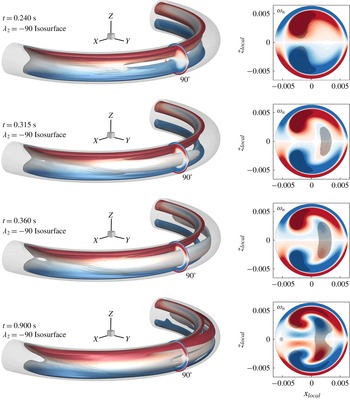
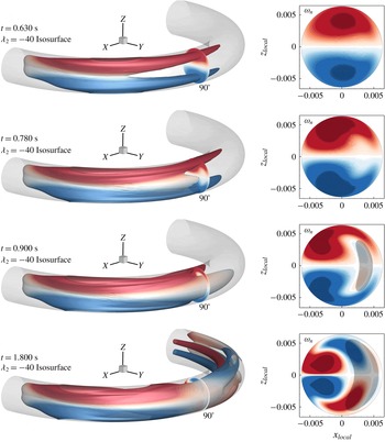
Figures 17 and 18 and supplementary movies 3 and 4 show the isosurface of
 $\unicode[STIX]{x1D706}_{2}$
at four instants in time for the moderate-step flow rate with no-slip and slip wall conditions, respectively. The isosurface is coloured by streamwise vorticity (
 $\unicode[STIX]{x1D714}_{n}$
) and the formation phases of the Lyne-type vortex are illustrated. At
 $90^{\circ }$
,
 $\unicode[STIX]{x1D714}_{n}$
is shown along with shaded regions that depict vortex cores detected by
 $\unicode[STIX]{x1D706}_{2}$
. The chosen isosurface and cross-sectional view show that the Lyne-type vortex displays weak
 $\unicode[STIX]{x1D714}_{n}$
but strong
 $\unicode[STIX]{x1D714}_{z}$
vorticity. In the location where
 $\unicode[STIX]{x1D714}_{n}$
is negligible (shown in grey/white colour) vorticity is mostly aligned in the
 $Z$
direction, and hence the white region on
 $\unicode[STIX]{x1D706}_{2}$
isosurface corresponds to high magnitude of
 $\unicode[STIX]{x1D714}_{z}$
.
Isosurface of
 $\unicode[STIX]{x1D706}_{2}=-90$
coloured by streamwise vorticity (
 $\unicode[STIX]{x1D714}_{n}$
) component for the moderate-step flow rate with no-slip wall condition at four instants in time. At
 $90^{\circ }$
,
 $\unicode[STIX]{x1D714}_{n}$
is shown and the shaded areas correspond to
 $\unicode[STIX]{x1D706}_{2}\leqslant -90$
, which identifies the vortex core regions. This figure shows the formation phase of the Lyne-type vortex. Movie 3 shows more phases and evolution in time.

According to figures 17 and 18 (and movies 3 and 4), the deformed-Dean vortex forms first prior to the Lyne-type vortex. The Lyne-type vortex forms at around
 $45^{\circ }$
at
 $t=0.024~\text{s}$
and then develops downstream for the no-slip wall condition. As discussed before, this process occurs later in time for the slip wall model at around the
 $60^{\circ }$
location. In these figures the isosurface of
 $\unicode[STIX]{x1D706}_{2}$
at the Lyne-type location during its formation is mostly white coloured, suggesting the vorticity axis in Lyne type at its origin is aligned with the
 $Z$
direction. This will be discussed later in further detail.
Isosurface of
 $\unicode[STIX]{x1D706}_{2}=-40$
coloured by streamwise vorticity (
 $\unicode[STIX]{x1D714}_{n}$
) component for the moderate-step flow rate with slip wall condition at four instants in time. At
 $90^{\circ }$
,
 $\unicode[STIX]{x1D714}_{n}$
is shown and the shaded areas correspond to
 $\unicode[STIX]{x1D706}_{2}\leqslant -40$
, identifying the vortex core region.

Application of almost any Eulerian-based vortex ID method involves some degree of subjectivity, because a threshold on the criterion must be defined. In the
 $\unicode[STIX]{x1D706}_{2}$
plots (figures 17 and 18) we have chosen the negative isosurface value such that it identifies the regions of interest. If all
 $\unicode[STIX]{x1D706}_{2}<0$
contours are plotted, all of these identified vortices will be connected together. In order to study this difficulty in more detail, various vortex ID methods are used, and for better illustrations, the identified vortices are mostly shown at the
 $90^{\circ }$
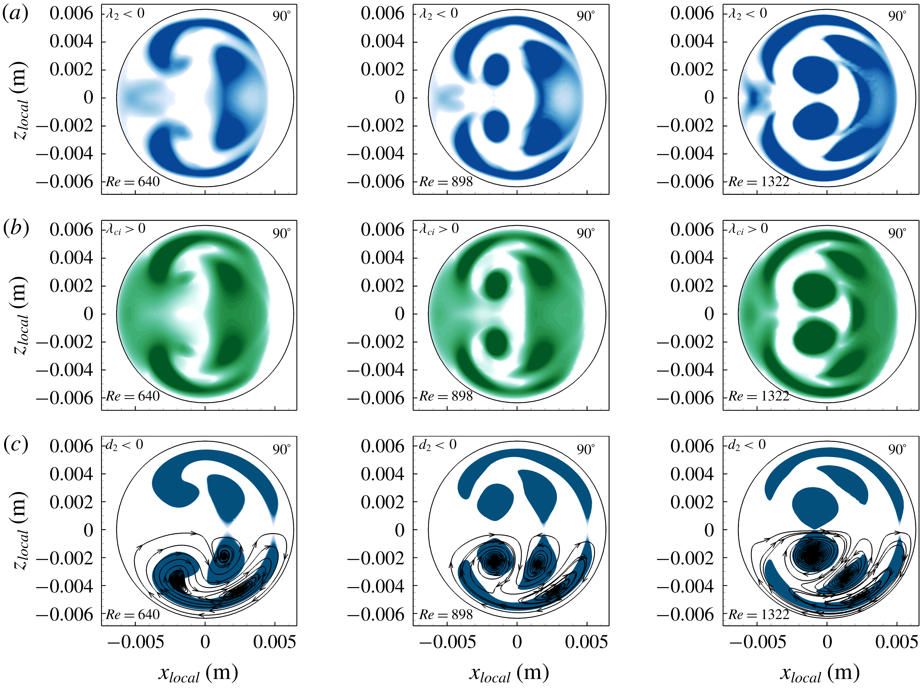
cross-section for steady-state conditions of moderate-step, mid-step and high-step flow rates. Figure 19 shows the identified vortices at
 $Re=640$
, 898 and 1322 via
 $\unicode[STIX]{x1D706}_{2}$
,
 $\unicode[STIX]{x1D706}_{ci}$
and
 $d_{2}$
. The thresholds were chosen objectively based on the definition of each method. The
 $\unicode[STIX]{x1D706}_{2}$
and
 $\unicode[STIX]{x1D706}_{ci}$
results, which are based on the 3-D data, show a connected region for all vortices, but
 $d_{2}$
results, based on 2-D cross-sectional in-plane data, show separated vortices. This suggests that those connecting regions that are not identified by the
 $d_{2}$
method have axes of rotation that lie in the cross-sectional plane (i.e. the plane of rotation is normal to the cross-sectional plane); therefore, it cannot be identified by the 2-D
 $d_{2}$
method. However, regions identified by the
 $d_{2}$
cannot be inferred to rotate solely in the cross-sectional planes, and might only have a weak rotational component in those planes.
Figure 19 also shows that the regions identified by
 $\unicode[STIX]{x1D706}_{2}$
and
 $\unicode[STIX]{x1D706}_{ci}$
are similar to each other, where
 $\unicode[STIX]{x1D706}_{2}$
provides a smaller area with more distinct vortices. Now the question arises: What is the axis of rotation for each vortex? Zhou et al. (Reference Zhou, Adrian, Balachandar and Kendall1999) and Chakraborty et al. (Reference Chakraborty, Balachandar and Adrian2005) suggested that if the velocity gradient tensor has a complex conjugate eigenpair of (
 $\unicode[STIX]{x1D706}_{cr}\pm \text{i}\unicode[STIX]{x1D706}_{ci}$
,
 $\unicode[STIX]{x1D742}_{cr}\pm \text{i}\unicode[STIX]{x1D742}_{ci}$
), where the
 $\unicode[STIX]{x1D742}_{cr}\pm \text{i}\unicode[STIX]{x1D742}_{ci}$
are eigenvectors associated with
 $\unicode[STIX]{x1D706}_{cr}\pm \text{i}\unicode[STIX]{x1D706}_{ci}$
, the plane spanned by the (
 $\unicode[STIX]{x1D742}_{cr},\unicode[STIX]{x1D742}_{ci}$
) is the plane of rotation. Therefore, the vector
 $\unicode[STIX]{x1D73B}_{n}=\unicode[STIX]{x1D742}_{cr}\times \unicode[STIX]{x1D742}_{ci}/(|\unicode[STIX]{x1D742}_{cr}||\unicode[STIX]{x1D742}_{ci}|)$
is parallel to the axis of rotation.
Vortex regions at the
 $90^{\circ }$
cross-section for three steady-state flow rates identified by (a)
 $\unicode[STIX]{x1D706}_{2}<0$
, (b)
 $\unicode[STIX]{x1D706}_{ci}>0$
and (c)
 $d_{2}<0$
. The
 $\unicode[STIX]{x1D706}_{2}$
and
 $\unicode[STIX]{x1D706}_{ci}$
values based on 3-D data show a connected region for identified vortices, and the
 $d_{2}$
method based on 2-D data shows separated identified vortices. Here 2-D streamlines are superimposed on the
 $d_{2}$
contour for illustration.

Since the
 $\unicode[STIX]{x1D706}_{2}$
and
 $\unicode[STIX]{x1D706}_{ci}$
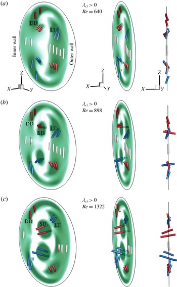
methods yield only scalar values and do not provide any information about the axis of rotation of each vortex, we identify the orientation of vortex axes by
 $\unicode[STIX]{x1D73B}_{n}$
. Figure 20 shows
 $\unicode[STIX]{x1D73B}_{n}$
vectors coloured by
 $\unicode[STIX]{x1D714}_{n}$
and contour plots of
 $\unicode[STIX]{x1D706}_{ci}>0$
at
 $90^{\circ }$
for three
 $Re$
. This figure shows that the axis of the identified vortex located near the centreline of the pipe (
 $Z=0~\text{m}$
) is mostly parallel to the
 $Z$
direction with insignificant streamwise vorticity (white vertical lines at the centre of the cross-section). Figure 20 also reveals that the Lyne-type vortex axis is mostly aligned with the
 $Z$
direction with a weak component in the streamwise direction. As
 $Re$
increases, the round-shaped head of the deformed-Dean vortex splits from its elongated part and the split-Dean vortex axis becomes more aligned with the streamwise direction.
Contours of
 $\unicode[STIX]{x1D706}_{ci}>0$
at the
 $90^{\circ }$
cross-section of the pipe for steady flows at (a)
 $Re=640$
, (b)
 $Re=898$
and (c)
 $Re=1322$
. The
 $\unicode[STIX]{x1D73B}_{n}$
vectors are parallel to the axis of rotation and are coloured by the streamwise vorticity (red lines anticlockwise and blue lines clockwise rotation). Three views shows the orientation of
 $\unicode[STIX]{x1D73B}_{n}$
vectors in three dimensions. DD, SD and LT refer to the deformed-Dean, split-Dean and Lyne-type vortices, respectively.

6.3 Lyne-type vortex
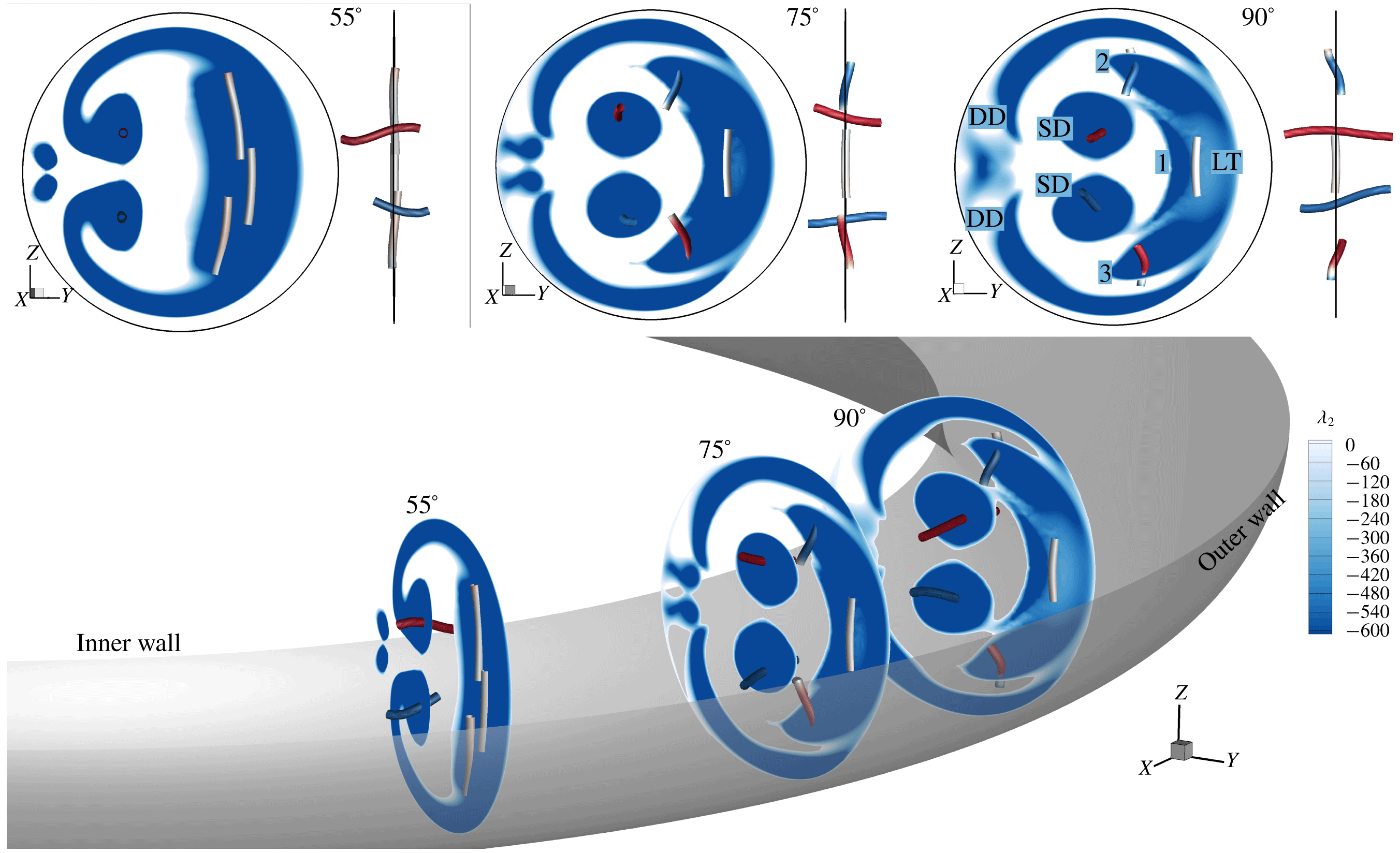
In order to determine the orientation of the Lyne-type vortex at its origin (the location in which it was formed initially), identified vortices are shown at multiple cross-sections in figure 21 for steady-state flow at the high-step flow rate. At
 $90^{\circ }$
,
 $\unicode[STIX]{x1D706}_{2}<0$
identifies three cores (dark blue) at the location of the Lyne-type vortex (shown by 1, 2 and 3) weakly connected, with a low magnitude of
 $\unicode[STIX]{x1D706}_{2}$
(light blue) in between. However, these three separate regions are strongly connected upstream at the
 $55^{\circ }$
cross-section and their axes of rotation are parallel and mostly aligned with the
 $Z$
direction. Therefore, the identified regions 1, 2 and 3 at the
 $90^{\circ }$
cross-section are part of one vortex upstream, rotating about an axis in the
 $Z$
direction. Figure 21 also shows that the spatial evolution of deformed-Dean vortex pairs through the curve and illustrates how the round-shaped head of the deformed-Dean vortex splits from its elongated part downstream of the
 $55^{\circ }$
cross-section and forms the split-Dean vortex system.
Cross-sectional views of
 $\unicode[STIX]{x1D706}_{2}<0$
for steady-state flow at
 $Re=1322$
. The
 $\unicode[STIX]{x1D73B}_{n}$
vectors are parallel to the axis of rotation and are coloured by the streamwise vorticity (red lines anticlockwise and blue lines clockwise rotation). Front and side views of cross-sections (a) and a 3-D view (b) of the curve are illustrated, demonstrating the evolution of the LT vortex and how its orientation changes and gains an axial component downstream of
 $55^{\circ }$
. DD, SD and LT refer to the deformed-Dean, split-Dean and Lyne-type vortices, respectively.

Looking at the
 $55^{\circ }$
cross-section in figure 21 may suggest that vortices (both deformed-Dean vortices and the Lyne-type vortex) that have configurations similar to two antiparallel vortices and one orthogonal vortex are also part of one structure. However, the high-step transient flow reveals more information about the interaction of these vortices at the
 $55^{\circ }$
cross-section.
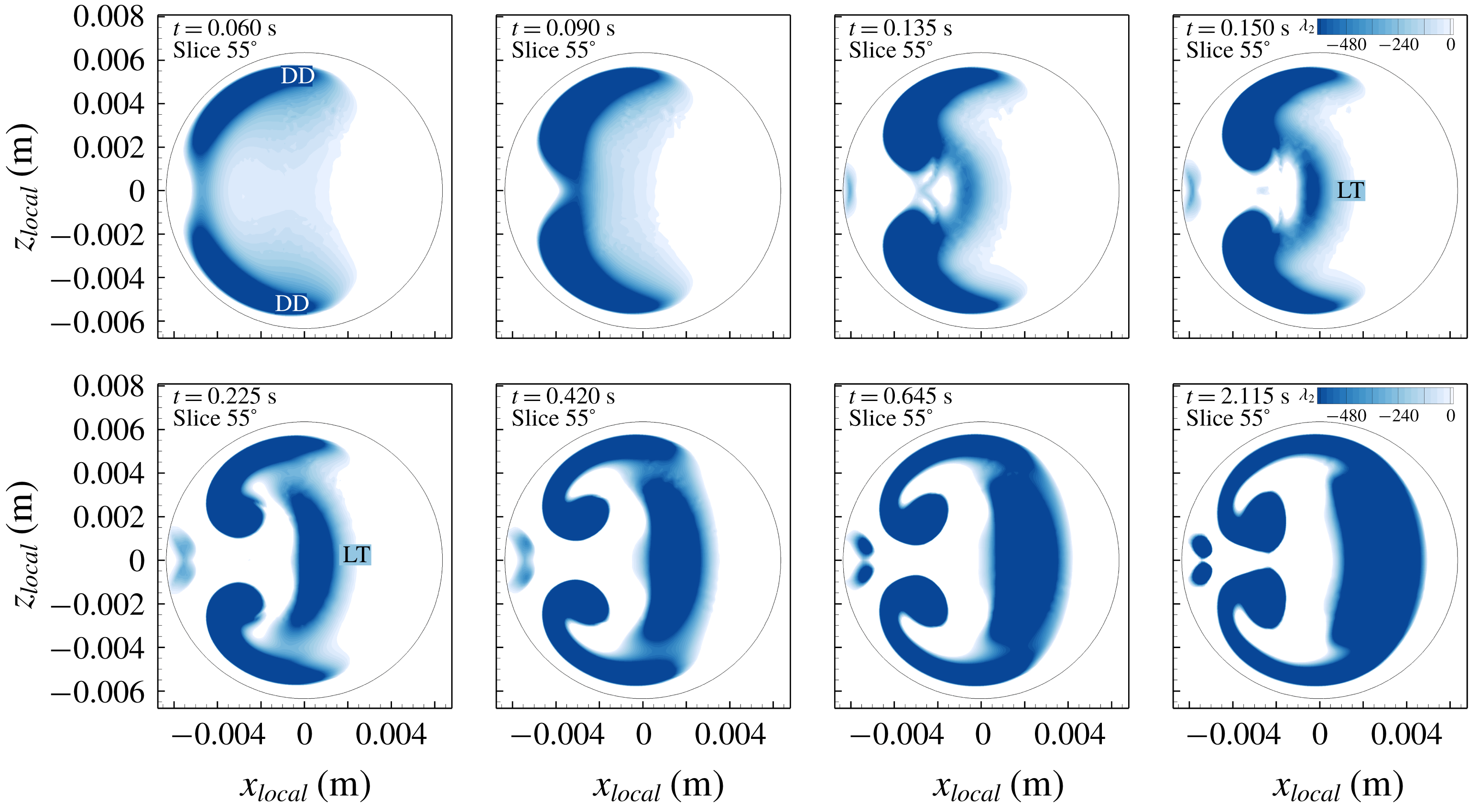
Figure 22 and movie 5 show
 $\unicode[STIX]{x1D706}_{2}<0$
at
 $55^{\circ }$
at eight phases during the high-step transient flow. At the early phases, two deformed-Dean vortices are detected. At
 $t=0.135~\text{s}$
the Lyne-type vortex starts to form near the centreline of the pipe and at
 $t=0.15~\text{s}$
the Lyne-type vortex is already formed at this cross-section. The Lyne-type vortex continues to grow in time while moving towards the outer wall until
 $t=0.645~\text{s}$
, where
 $\unicode[STIX]{x1D706}_{2}$
shows a connected region of Lyne-type and deformed-Dean vortices. After this phase, the
 $\unicode[STIX]{x1D706}_{2}$
plot is similar to the
 $55^{\circ }$
cross-section in figure 21. Therefore, figure 22 suggests that the Lyne-type vortex is different from the classical deformed-Dean vortices because the Lyne-type vortex formed later in time and was distinct from the deformed-Dean vortices seen at the beginning. However, the deformed-Dean vortices still play a role in the formation of the Lyne-type vortex.
Contours of
 $\unicode[STIX]{x1D706}_{2}<0$
at
 $55^{\circ }$
at eight phases during the high-step transient flow. This figure shows that only the deformed-Dean (DD) vortices existed at the beginning of the flow. Later in time at
 $t=0.135~\text{s}$
, the Lyne-type (LT) vortex is forming. Towards the end at steady-state condition,
 $\unicode[STIX]{x1D706}_{2}$
shows a connected region of three vortices (in dark blue).

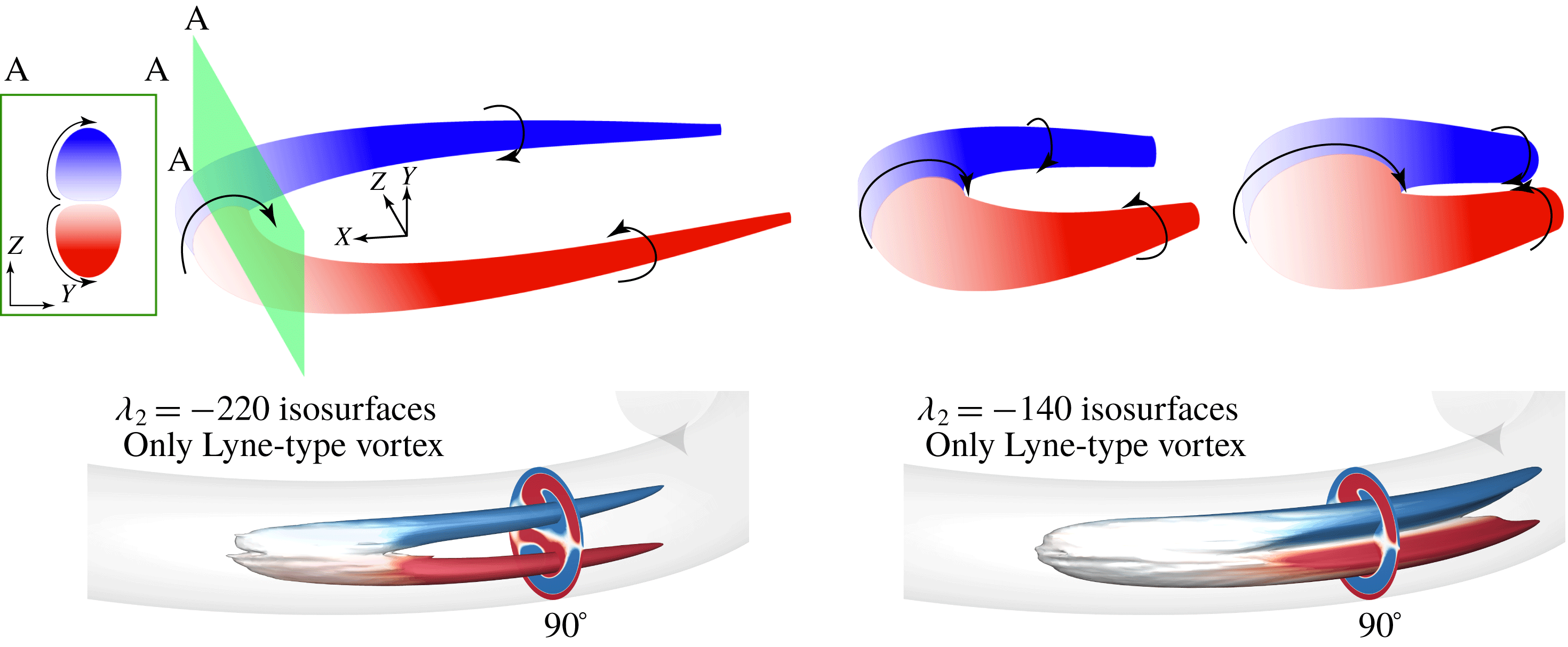
After analysing and determining the orientation of the Lyne-type vortex, it is necessary to discuss its uncommon shape based on 3-D vortex ID results. Figure 23 shows a schematic of a vortex on the left that is similar to the well-known hairpin vortex. The colour denotes the streamwise vorticity, where red and blue represent positive and negative vorticity, respectively. If the plane of investigation cuts through the head of this vortex (section A–A) the cross-sectional view shows two counter-rotating vortices and zero streamwise vorticity near the centreline (white region between section A–A). Since the head of this vortex rotates about the
 $Z$
direction, the cross-sectional view does not detect any vorticity at the centreline, so a 2-D vortex ID method will detect only two separate regions. However, if a 3-D vortex ID method is used, it will detect one connected region. If the head of this vortex stretches so that it connects the area between its legs (similar to the rightmost vortex in figure 23), vorticity in any cross-sectional view is similar to the cross-section A–A. This is the model of the Lyne-type vortex whose primary axis of rotation is in the
 $Z$
direction (figure 21,
 $55^{\circ }$
cross-section) and if we cut downstream of the head, three connected cores can be detected (regions 1, 2 and 3 in figure 21,
 $90^{\circ }$
cross-section). In figure 23, the isosurfaces of the Lyne-type vortex are shown at two values (
 $\unicode[STIX]{x1D706}_{2}=-220$
and
 $\unicode[STIX]{x1D706}_{2}=-140$
) to illustrate the correspondence between the schematic and the actual vortex.
Now that the orientation and morphology of the Lyne-type vortex have been determined, we can compare it to the vortex system originally reported by Lyne (Reference Lyne1971). To study the classical Lyne vortex, oscillatory flow with
 $\unicode[STIX]{x1D6FC}=17$
was simulated and the results are presented in appendix A. There are major differences between the Lyne-type vortex in steady, transient or pulsatile flows and the original classical Lyne vortex pair in oscillatory flow. The main difference is that the rotation axis of the Lyne vortex is aligned with the streamwise direction, whereas the Lyne-type vortex axis is oriented mostly in the
 $Z$
direction. The Lyne vortex forms slowly in the inviscid region of the flow, while the Lyne-type vortex has significant vorticity magnitude that was delivered via vorticity convection and vortex stretching. Another major difference is revealed by the
 $\unicode[STIX]{x1D706}_{2}$
method, which cannot detect the Lyne vortex but can detect the Lyne-type vortex, suggesting that there is a fundamental difference between these two vortices. Therefore, the Lyne-type vortex reported in previous studies (e.g. Boiron et al.
Reference Boiron, Deplano and Pelissier2007; Glenn et al.
Reference Glenn, Bulusu, Shu and Plesniak2012; van Wyk et al.
Reference van Wyk, Prahl Wittberg, Bulusu, Fuchs and Plesniak2015; Najjari et al.
Reference Najjari, Hinke, Bulusu and Plesniak2016) is not the same as the Lyne vortex in oscillatory flow despite their visual similarities in 2-D cross-sectional slices. Fully 3-D data coupled with vortex ID methods were required to elucidate this structure in pulsatile flows.
Schematic of a vortex (similar to the hairpin vortex) in which the vortex head grows and its legs approach one another to the point where the vortex head stretches and fills the area between the legs. The colour denotes the streamwise vorticity and section A–A is cutting through the vortex head. At the centre, the rotation of the head is purely in the
 $X$
–
 $Y$
plane (along the
 $Z$
direction). This schematic represents the Lyne-type vortex. The simulated Lyne-type vortex, for
 $Re=640$
illustrated by
 $\unicode[STIX]{x1D706}_{2}$
isosurfaces of
 $\unicode[STIX]{x1D706}_{2}=-220$
and
 $\unicode[STIX]{x1D706}_{2}=-140$
and coloured by
 $\unicode[STIX]{x1D714}_{n}$
, demonstrates its morphology.

6.4 Vortex circulation
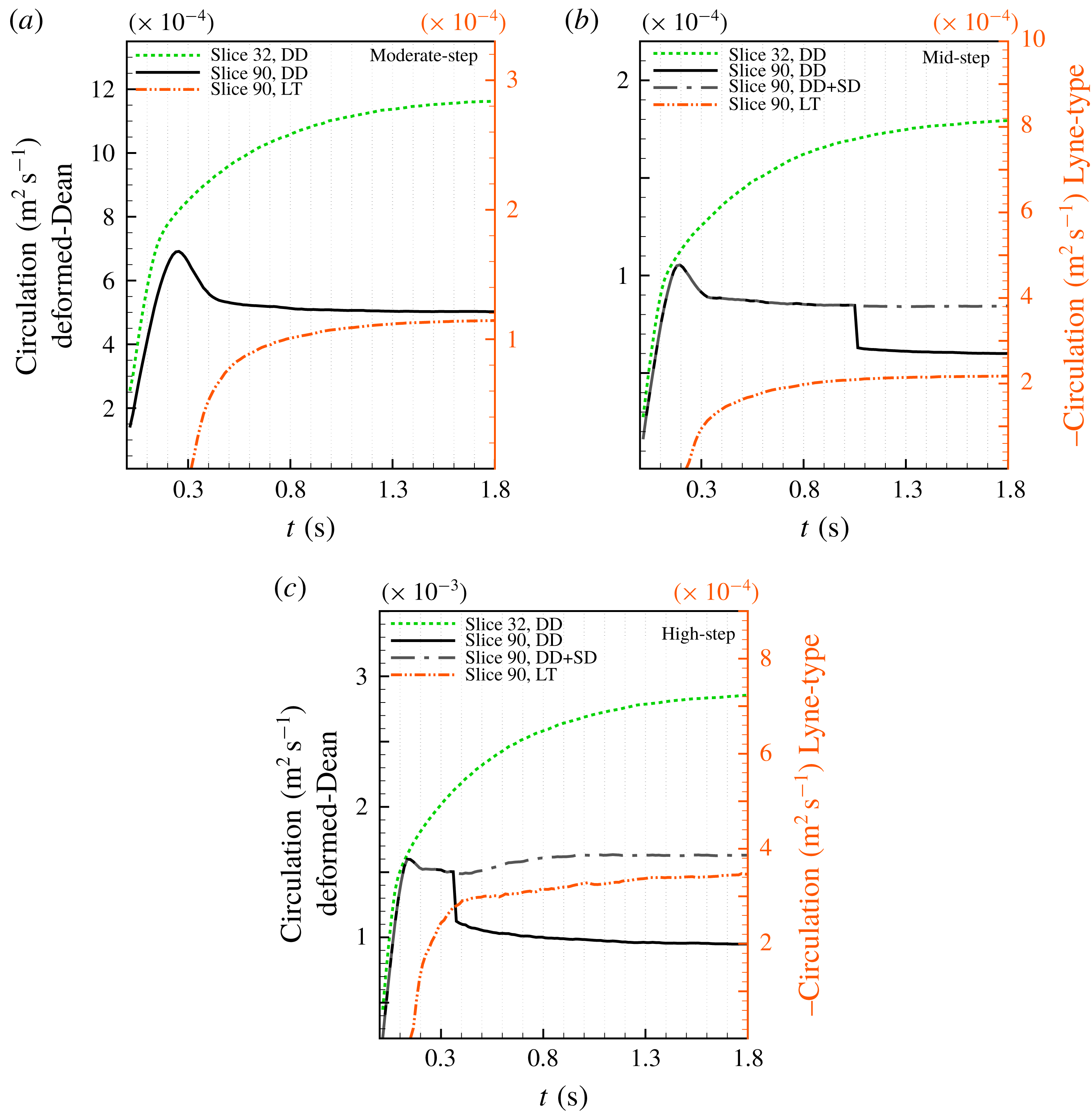
Figure 24 plots the circulation (
 $\unicode[STIX]{x1D6E4}$
) of each vortex, calculated by (5.1) associated with the rotation in the secondary flow direction regardless of the actual vortex orientation. This helps us to investigate the formation time of vortices and is not necessarily correlated to the total vortex strength, because the main orientation of the Lyne-type vortex, for example, is not in the streamwise direction and
 $d_{2}$
, which identifies the vortex region for
 $\unicode[STIX]{x1D6E4}$
, only detects part of this vortex. Firstly, since the Lyne-type vortex axis is weakly aligned in the streamwise direction, the
 $d_{2}$
method (based on 2-D cross-sectional data) cannot detect the Lyne-type vortex when the flow rate is low. Secondly, circulation of the Lyne-type vortex in the cross-section is lower than that of the deformed-Dean vortex.
Circulation of each vortex at
 $32^{\circ }$
and
 $90^{\circ }$
calculated in the cross-sections (in upper half of the cross-section,
 $Z>0$
) with no-slip wall condition, for (a) moderate-step flow, (b) mid-step flow and (c) high-step flow rate. Each plot shows the formation time of various vortices obtained by methods explained in § 5. The area of the vortex was defined by the
 $d_{2}$
method and
 $\unicode[STIX]{x1D714}_{n}$
was used in the summation in (5.1). Deformed-Dean, split-Dean and Lyne-type vortices are designated by DD, SD and LT, respectively. After the SD was split from the DD vortex, the grey (coloured) dashed-dotted lines represent the summation of SD and DD circulations.

Figure 24 shows that vortices form earlier in time by increasing
 $Re$
from moderate-step to high-step flow rate. The Lyne-type vortex at
 $90^{\circ }$
forms at around
 $t=0.3~\text{s}$
and
 $t=0.15~\text{s}$
for moderate-step and high-step flows, respectively. Similarly, the deformed-Dean vortex forms quickly for higher flow rates and, by increasing the step flow rate,
 $\unicode[STIX]{x2202}\unicode[STIX]{x1D6E4}/\unicode[STIX]{x2202}t$
also increases. The phase of peak circulation of the deformed-Dean vortex also occurs earlier in time; for the moderate-step flow rate the peak in deformed-Dean circulation is at
 $t\simeq 2.5~\text{s}$
, whereas the peak for high-step flow rate occurs at
 $t\simeq 1.5~\text{s}$
, which is related to the formation of the Lyne-type vortex. It was discussed that during formation of the Lyne-type vortex, the deformed-Dean vortex was pushed away from the centre of the pipe by the Lyne-type vortex, causing a reduction in the area occupied by the deformed-Dean vortex. This is the reason why the circulation of the latter has a peak/plateau immediately before the appearance of the Lyne-type vortex in the cross-sections. However, this trend is absent in the
 $32^{\circ }$
cross-section and the circulation monotonically increases over time. It was also discussed that the Lyne-type vortex forms downstream of
 $30^{\circ }$
; therefore, at the
 $32^{\circ }$
location (in figure 24) the Lyne-type vortex has not formed in the cross-section and cannot affect the circulation of the deformed-Dean vortex. In figure 24, for mid-step and high-step flow rates when the split-Dean vortex forms after splitting, the aggregate circulation of deformed-Dean and split-Dean follows the trend of deformed-Dean circulation before splitting. So, two vortices maintain their relative rotation after splitting in steady flow. The results also show that splitting occurs sooner for high-step flow rate when compared to mid-step flow rate. Several mechanisms responsible for vortex splitting and formation of the split-Dean vortex from deformed-Dean were discussed in Cox (Reference Cox2017) and are not the focus of the current study.
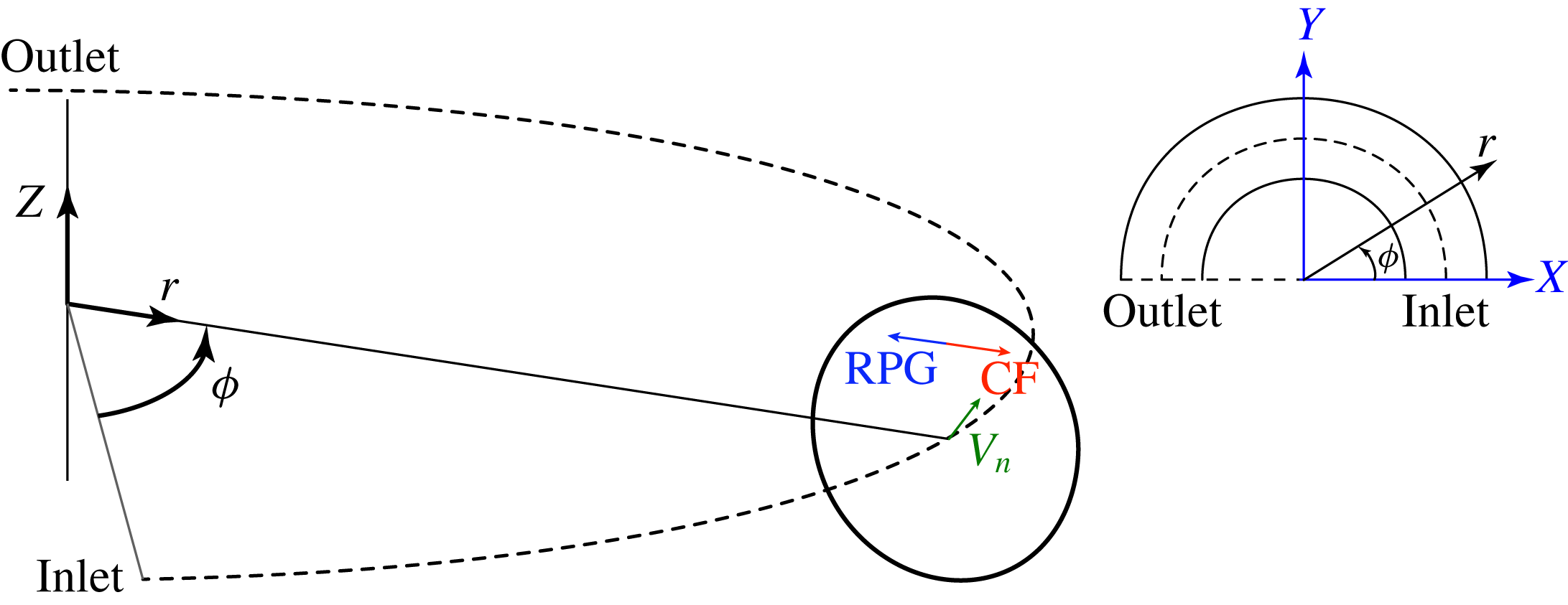
Cylindrical coordinate orientation. The centrifugal and radial pressure gradient forces are shown schematically in the cross-section.

6.5 Analysis and further discussion
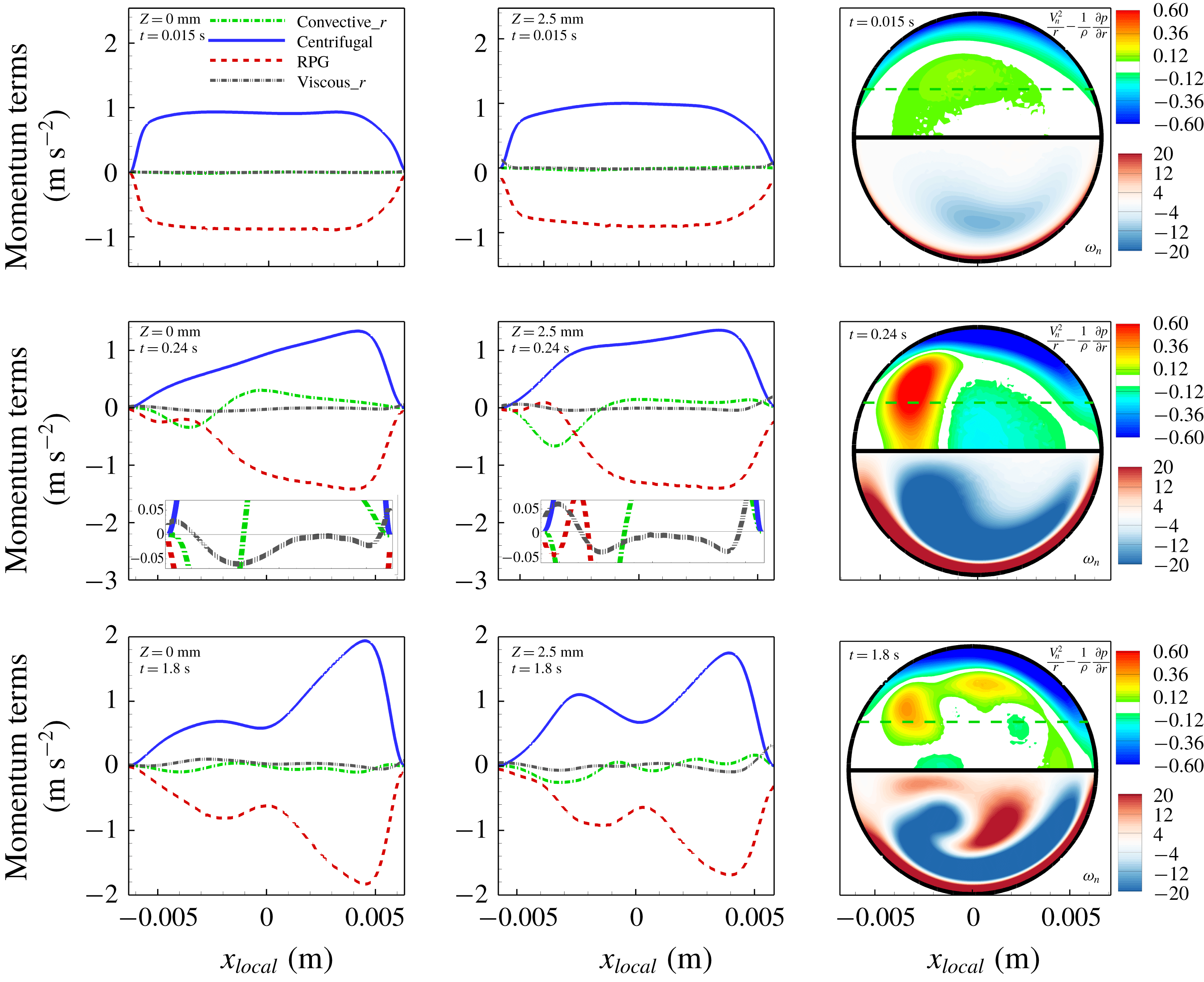
In this section the flow dynamics of both moderate-step flow and pure oscillatory flow (where a classical Lyne vortex pair forms) are investigated. Appendix A fully describes the velocity, vorticity and vortex ID results under pure oscillatory flow where the classical Lyne vortex is revisited and analysed with the new vortex ID method. It is known that the centrifugal force plays an important role in generating Dean vortices, and the balance of centrifugal and radial pressure gradient forces has been investigated in several studies, e.g. Boiron et al. (Reference Boiron, Deplano and Pelissier2007) and Alastruey et al. (Reference Alastruey, Siggers, Peiffer, Doorly and Sherwin2012). While the current numerical results were obtained by solving the governing equations in Cartesian coordinates, other researchers have used toroidal coordinates to simulate flow in a curved pipe. However, the centrifugal force does not appear in the momentum equation in Cartesian coordinates, and the pure centrifugal force term only appears on the centreline (
 $z=0$
) in toroidal coordinates (Boiron et al.
Reference Boiron, Deplano and Pelissier2007). To circumvent this issue, cylindrical coordinates are used to provide the centrifugal force at any point in the cross-sections without being limited only to the symmetry plane. Figure 25 shows the coordinate system used for our momentum balance and (6.2) and (6.3) describe the relation between Cartesian and cylindrical coordinates for
 $0^{\circ }<\unicode[STIX]{x1D719}<180^{\circ }$
:
 $$\begin{eqnarray}\displaystyle & \displaystyle \left.\begin{array}{@{}c@{}}X=r\cos \unicode[STIX]{x1D719},\\ Y=r\sin \unicode[STIX]{x1D719},\\ r=\sqrt{X^{2}+Y^{2}},\end{array}\right\} & \displaystyle\end{eqnarray}$$
 $$\begin{eqnarray}\displaystyle & \displaystyle \left.\begin{array}{@{}c@{}}V_{r}=u\cos \unicode[STIX]{x1D719}+v\sin \unicode[STIX]{x1D719},\\ V_{\unicode[STIX]{x1D719}}=V_{n}=-u\sin \unicode[STIX]{x1D719}+v\cos \unicode[STIX]{x1D719}.\end{array}\right\} & \displaystyle\end{eqnarray}$$
In cylindrical coordinates the
 $r$
-momentum equation provides the centrifugal and radial pressure gradient (RPG) explicitly. Since the simulations were performed in Cartesian coordinates, velocity and pressure gradients are available with respect to
 $X$
,
 $Y$
and
 $Z$
. Therefore, the
 $r$
-momentum equation is transformed and written based on derivatives in Cartesian coordinates. To obtain the proper transformed equation shown in (6.4), the chain rule, directional derivatives and the equations cast in cylindrical coordinates were used:
 $$\begin{eqnarray}\displaystyle \frac{\unicode[STIX]{x2202}V_{r}}{\unicode[STIX]{x2202}t} & = & \displaystyle \frac{1}{r}\left(u^{2}\sin ^{2}\unicode[STIX]{x1D719}+v\left(v\cos ^{2}\unicode[STIX]{x1D719}+X\frac{\unicode[STIX]{x2202}u}{\unicode[STIX]{x2202}Y}+Y\frac{\unicode[STIX]{x2202}v}{\unicode[STIX]{x2202}Y}\right)\right.\nonumber\\ \displaystyle & & \displaystyle +\left.u\left(-v\sin 2\unicode[STIX]{x1D719}+X\frac{\unicode[STIX]{x2202}u}{\unicode[STIX]{x2202}X}+Y\frac{\unicode[STIX]{x2202}v}{\unicode[STIX]{x2202}X}\right)\right)+w\frac{\unicode[STIX]{x2202}V_{r}}{\unicode[STIX]{x2202}Z}+\frac{V_{n}^{2}}{r}-\frac{1}{\unicode[STIX]{x1D70C}}\frac{\unicode[STIX]{x2202}p}{\unicode[STIX]{x2202}r}\nonumber\\ \displaystyle & & \displaystyle +\,\unicode[STIX]{x1D708}\left(\left(\frac{\unicode[STIX]{x2202}^{2}u}{\unicode[STIX]{x2202}X^{2}}+\frac{\unicode[STIX]{x2202}^{2}u}{\unicode[STIX]{x2202}Y^{2}}+\frac{\unicode[STIX]{x2202}^{2}u}{\unicode[STIX]{x2202}Z^{2}}\right)\cos \unicode[STIX]{x1D719}+\left(\frac{\unicode[STIX]{x2202}^{2}v}{\unicode[STIX]{x2202}X^{2}}+\frac{\unicode[STIX]{x2202}^{2}v}{\unicode[STIX]{x2202}Y^{2}}+\frac{\unicode[STIX]{x2202}^{2}v}{\unicode[STIX]{x2202}Z^{2}}\right)\sin \unicode[STIX]{x1D719}\right).\end{eqnarray}$$
The first two terms on the right-hand side in (6.4) indicate the convective force in the
 $r$
direction, while the second (
 $V_{n}^{2}/r$
) and third (
 $-(1/\unicode[STIX]{x1D70C})\,\unicode[STIX]{x2202}p/\unicode[STIX]{x2202}r$
) terms are centrifugal and radial pressure gradient forces, respectively. The last term corresponds to the viscous force in the
 $r$
direction. The radial pressure gradient can be written based on derivatives with respect to
 $X$
and
 $Y$
in (6.5), and
 $\unicode[STIX]{x2202}V_{r}/\unicode[STIX]{x2202}Z=\cos \unicode[STIX]{x1D719}\,\unicode[STIX]{x2202}u/\unicode[STIX]{x2202}Z+\sin \unicode[STIX]{x1D719}\,\unicode[STIX]{x2202}v/\unicode[STIX]{x2202}Z$
:
 $$\begin{eqnarray}-\frac{1}{\unicode[STIX]{x1D70C}}\frac{\unicode[STIX]{x2202}p}{\unicode[STIX]{x2202}r}=-\frac{1}{\unicode[STIX]{x1D70C}}\left(\frac{\unicode[STIX]{x2202}p}{\unicode[STIX]{x2202}X}\frac{\unicode[STIX]{x2202}X}{\unicode[STIX]{x2202}r}+\frac{\unicode[STIX]{x2202}p}{\unicode[STIX]{x2202}Y}\frac{\unicode[STIX]{x2202}Y}{\unicode[STIX]{x2202}r}\right).\end{eqnarray}$$
Equation (6.4) is applicable at any point in the flow and the force balance at the
 $90^{\circ }$
cross-section can be obtained using (6.6), where
 $r$
and
 $V_{r}$
can be substituted by
 $Y$
and
 $v$
, respectively:
 $$\begin{eqnarray}\frac{\unicode[STIX]{x2202}v}{\unicode[STIX]{x2202}t}=-\left(\frac{u^{2}}{Y}+u\frac{\unicode[STIX]{x2202}v}{\unicode[STIX]{x2202}X}+v\frac{\unicode[STIX]{x2202}v}{\unicode[STIX]{x2202}Y}+w\frac{\unicode[STIX]{x2202}v}{\unicode[STIX]{x2202}Z}\right)+\frac{u^{2}}{Y}-\frac{1}{\unicode[STIX]{x1D70C}}\frac{\unicode[STIX]{x2202}p}{\unicode[STIX]{x2202}Y}+\unicode[STIX]{x1D708}\left(\frac{\unicode[STIX]{x2202}^{2}v}{\unicode[STIX]{x2202}X^{2}}+\frac{\unicode[STIX]{x2202}^{2}v}{\unicode[STIX]{x2202}Y^{2}}+\frac{\unicode[STIX]{x2202}^{2}v}{\unicode[STIX]{x2202}Z^{2}}\right).\end{eqnarray}$$
Momentum balance in
 $r$
direction on
 $Z=0$
and
 $Z=2.5~\text{mm}$
lines at
 $\unicode[STIX]{x1D719}=90^{\circ }$
for moderate-step flow rate. Balance of centrifugal force and radial pressure gradient is shown in the top half of the cross-section and streamwise vorticity is shown in the bottom half. The horizontal dashed line shows
 $Z=2.5~\text{mm}$
.

Figure 26 shows the force balance in
 $r$
direction at the
 $90^{\circ }$
cross-section of the pipe on two horizontal lines (
 $Z=0$
and 2.5 mm). The cross-sectional view shows the balance of centrifugal and radial pressure gradient terms. At
 $t=0.015~\text{s}$
, the flow is accelerating and the velocity profile has not developed yet and is similar to a plug flow profile at
 $90^{\circ }$
. This causes the centrifugal force profile to be almost flat in the core region and balanced by RPG. During the transient flow at
 $t=0.24~\text{s}$
, the Lyne-type vortex forms, and similar to what Boiron et al. (Reference Boiron, Deplano and Pelissier2007) observed, the RPG dominates the centrifugal term at the location of the Lyne-type vortex. During the transient flow, the convective term is significant, and near the inner wall region its magnitude is comparable to centrifugal and RPG terms. At this time, near the inner wall (at
 $x_{local}\approx -4~\text{mm}$
and
 $Z=2.5~\text{mm}$
) where the deformed-Dean vortex is located, the RPG is small and even becomes positive (exerting force towards the outer wall). The small, positive values of RPG (
 $-(1/\unicode[STIX]{x1D70C})\,\unicode[STIX]{x2202}p/\unicode[STIX]{x2202}r$
) in this region are attributable to the local pressure minimum in the core of the deformed-Dean vortex.
Momentum balance in
 $r$
direction on
 $Z=0$
and
 $Z=2.5~\text{mm}$
lines at
 $\unicode[STIX]{x1D719}=90^{\circ }$
for oscillatory Lyne flow. Balance of centrifugal force and radial pressure gradient is shown in the top half of the cross-section and streamwise vorticity is shown in the bottom half. The horizontal dashed line shows
 $Z=2.5~\text{mm}$
.

The force balance in
 $r$
direction for the oscillatory flow (classical Lyne problem) is shown in figure 27, which illustrates that the centrifugal and pressure gradient forces are well balanced by each other. Insets in figures 26 and 27 show that the viscous force is near zero for both oscillatory Lyne and moderate-step flow except at the near-wall regions. Also, the convective term is near zero for the oscillatory Lyne case as well, but non-zero for moderate-step flow where Lyne-type vortex forms. This convective term may have a role in formation of the Lyne-type vortex.
7 Summary and conclusions
Flow inside a
 $180^{\circ }$
curved pipe was studied via PIV experiments and CFD simulations. The results of numerical simulations match well with our PIV experiments. To study the temporal and spatial evolution of vortices in a curved pipe, three transient impulsively started step-like flows were introduced at the inlet, and the developing flow was studied in the curved section. Several vortex ID criteria were used in this study to detect coherent secondary flow vortical structures, and their results were compared. The vorticity transport equation was analysed to track the origin of vorticity in the Lyne-type vortex. A pure oscillatory flow (classical Lyne experiment) was also investigated to compare the Lyne vortex pair with the Lyne-type vortex under steady, transient or pulsatile flows and to distinguish the differences in the structures that form under various conditions.
Our analysis revealed that the vorticity in the Lyne-type vortex is transported via convection from the inner wall region during its formation phases. In a pipe with the (idealized) slip wall model, the Lyne-type vortex was also detected; however, it was weaker and formed later in time compared to results from the no-slip condition. Its vorticity originated from the vorticity introduced by the physical velocity profile at the inlet rather than at the wall in the curved section (where vorticity could not be generated because of the inviscid boundary condition).
The results of vortex ID methods identified the source of the Lyne-type vortex, while calculating eigenvalues and eigenvectors of the velocity gradient tensor revealed the vortex axis orientation. Temporal and spatial evolution of various vortical structures were also illustrated by vortex ID methods. The analysis showed that the Lyne-type vortex (in pulsatile and steady flows), which was previously identified as two counter-rotating vortices (one vortex pair) by 2-D vortex ID or streamlines in the cross-section, is actually one structure with an axis of rotation primarily in the
 $Z$
direction. The Lyne-type vortex morphology is similar to a hairpin vortex in which the head has grown and stretched such that it connects the regions between its legs. Therefore, the previously reported cross-sectional vortex pattern (visually similar to the Lyne vortex pair in oscillatory flows) is actually a single vortex with a projection on the cross-section that appears as two separate counter-rotating vortices when identified by 2-D vortex ID methods or streamlines. This is a different structure than the Lyne vortex pair and is defined here as Lyne-type from a historical perspective due to the visual similarity to the original Lyne structure.
Additionally, new analysis of the Lyne vortex pair in pure oscillatory flow showed that the Lyne vortex rotation axis is mostly aligned with the streamwise direction with small vorticity magnitude. The
 $\unicode[STIX]{x1D706}_{2}$
vortex ID method could not detect the Lyne vortex pair. Moreover, the axial (streamwise) velocity profile in the Lyne vortex region is almost flat, which is an indication of an inviscid region, whereas no such inviscid region exists in pulsatile/steady flow. These classical Lyne vortex characteristics are different from those of the Lyne-type vortex in steady, transient and pulsatile flows, making it a distinctly different structure than the Lyne vortex pair. This is mainly because the oscillatory flow has to stop and reverse during its period, which prevents the viscous region from developing in the core of the pipe; whereas in pulsatile and steady flows the positive net flow rate causes the viscous region to develop into the core. The existence of a viscous core significantly affects the flow behaviour and leads to formation of the Lyne-type vortex in steady/pulsatile flows, and produces a strong
 $Z$
vorticity component. In contrast, the original Lyne vortex pair displays negligible vorticity in the
 $Z$
direction under oscillatory flow.
Acknowledgements
This study was supported by The George Washington University Center for Biomimetics and Bioinspired Engineering. The first author also acknowledges the support provided by the Frank and Marcia Mau Annual Scholarship Award and the Department of Mechanical and Aerospace Engineering; and the second author acknowledges support under The George Washington University Presidential Merit Fellowship.
Supplementary movies
Supplementary movies are available at https://doi.org/10.1017/jfm.2019.510.
Appendix A. New analysis of the Lyne problem in pure oscillatory flow
It was discussed in the paper that 2-D cross-sectional data of pulsatile or steady flows in a curved pipe (e.g.
 $d_{2}$
and streamlines in figure 19) may suggest that extra vortices are part of the Lyne vortex system. To investigate this assertion, the Lyne study was revisited here with pure oscillatory flow with Womersley number
 $\unicode[STIX]{x1D6FC}=17$
, maximum
 $Re=700$
and maximum
 $De=265$
, and period of
 $T=0.25~\text{s}$
. Figure 28 shows the flow rate used for the Lyne simulations, which were performed for a total of 14 full cycles (equivalent to 28 cycles since the flow rate is oscillatory, and the positive and negative portions have identical effects). These 14 full cycles are sufficient to reach cycle-to-cycle convergence and eliminate the effect of the initial condition, and figure 29 shows this convergence. Velocity magnitude and secondary velocity magnitude were averaged for the entire field at fixed phases (p1–p4) and results are plotted for the indicated number of cycles in figure 29. Wall shear stress (WSS) was also averaged on the boundary of the pipe at the same phases and plotted. The vorticity magnitude cycle-to-cycle convergence averaging was performed in the regions where
 $r<4.5~\text{mm}$
to eliminate the effect of dominant vorticity near the wall. Figure 29 shows that the variation of these quantities between cycles 13 and 14 is less than 0.2 %. Thus at the fourteenth cycle the results are converged and are cycle-invariant. All of the results presented for Lyne flow are for cycle 14, except where otherwise noted.
Oscillatory flow rate for Lyne simulation with cycle period of
 $T=0.25~\text{s}$
, frequency of
 $f=4~\text{Hz}$
and Womersley number of
 $\unicode[STIX]{x1D6FC}=17$
. The upper axis (
 $t_{14}$
) shows the physical time of cycle 14. The cycle-to-cycle convergence, shown in figure 29, was calculated at four phases (p1–p4) during the cycle.

Convergence of the averaged (a) velocity magnitude, (b) secondary velocity magnitude, (c) vorticity magnitude at
 $r<4.5~\text{mm}$
and (d) wall shear stress. The quantity
 $e=(|m_{i}-m_{14}|/m_{14})\times 100$
shows the differences of the averaged parameter in previous cycles with the quantities in the last (fourteenth) cycle. The parameter
 $m$
refers to an averaged quantity (e.g. velocity magnitude) and
 $i$
represents the cycle number.

Previous studies represented the Lyne vortex pair by streamlines or streamwise vorticity in the cross-sectional view in addition to line plots of axial velocity and vorticity profiles. Figure 30 shows
 $\unicode[STIX]{x1D714}_{n}$
, secondary streamlines and axial velocity profiles on the centreline at
 $90^{\circ }$
. These results agree well with those of Siggers & Waters (Reference Siggers and Waters2008). In the simulation with high Womersley number,
 $\unicode[STIX]{x1D6FC}=17$
, the flow is found to be independent of the axial location in the curved section between
 $35^{\circ }\leqslant \unicode[STIX]{x1D719}\leqslant 145^{\circ }$
, i.e. the flow is fully developed in the curve. In contrast, the steady/transient flows in the current study are not fully developed in the curve. This is another significant difference between oscillatory and steady/pulsatile flows in curved pipes.
Streamwise vorticity (
 $\unicode[STIX]{x1D714}_{n}$
) contours and secondary velocity streamlines at
 $90^{\circ }$
for four instants in time during pure oscillatory flow in the Lyne simulation with
 $\unicode[STIX]{x1D6FC}=17$
and maximum
 $Re=700$
. The axial (streamwise) velocity profile is plotted along the horizontal diameter (black) line, and
 $\unicode[STIX]{x1D714}_{n}$
is plotted along the vertical radius (blue line). The labels DD and L denote the deformed-Dean and Lyne vortices, respectively. Results agree well with those in Siggers & Waters (Reference Siggers and Waters2008). More phases are illustrated in supplementary movie 6.

To investigate temporal evolution of vortices in oscillatory flow, swirling strength (
 $\unicode[STIX]{x1D706}_{ci}$
) was used to identify vortex regions and the vector
 $\unicode[STIX]{x1D73B}_{n}$
was calculated to determine the axis of rotation. Figure 31 shows
 $\unicode[STIX]{x1D706}_{ci}>0$
regions for nine phases during the first half of the fourteenth cycle (
 $3.25\leqslant t<3.375$
). In figure 31(a) three regions (1, 2, 3) were labelled to trace their temporal evolution. Region 1 refers to the deformed-Dean vortices for which the rotation axis has a strong component in the
 $Z$
direction. As the cycle progresses, region 1 moves away from the outer wall and slowly shifts towards the interior of the cross-section (figure 31
a–f). During this transition, the orientation of the vortex 1 axis (
 $\unicode[STIX]{x1D73B}_{n}$
) becomes more closely aligned with the streamwise direction (figure 31
f). At
 $t=3.36~\text{s}$
, figure 31(g), a new region of
 $\unicode[STIX]{x1D706}_{ci}>0$
appears near the outer wall, which is labelled as 1, and the previous region 1 has moved away from the wall and is designated by 2. In figure 31(h), a new region appears near the centre of the pipe, marked by 3. This region grows in time as shown in figure 31(i), where regions 1, 2 and 3 are similar to figure 31(a). At
 $t=3.375~\text{s}$
or
 $t/T=0.5$
this whole process repeats again for the next half of the cycle. Owing to the short cycle period, the deformed-Dean vortex pair from one cycle persists to the next cycle, where it interacts with the Lyne vortex near the pipe centreline. Consequently, region 2 in figure 31(a–c) contains of deformed-Dean vortices from the previous half-cycle. The axis of rotation in region 2 is primarily in the streamwise direction, and based on
 $\unicode[STIX]{x1D706}_{ci}$
, this region is merged with region 3 (the Lyne vortex).
Figure 31 also shows that the axis of the Lyne vortex is mostly in the streamwise direction even though its strength and vorticity are considerably lower compared to those of the deformed-Dean vortex. Although we showed that regions 2 and 3 are part of the Lyne vortex with
 $\unicode[STIX]{x1D706}_{ci}$
criterion,
 $\unicode[STIX]{x1D706}_{ci}>0$
does not detect any vortical activity in the core region for some phases (at which the
 $V_{n}$
is large) during the cycle. On the other hand, streamlines always show a spiral pattern that is consistent with the classical description of the Lyne vortex reported in the literature. Various vortex ID methods are compared next to investigate the classical description of Lyne vortex pair using 3-D and 2-D vortex ID methods. This extends previously published results concerning this classical problem.
Three-dimensional and side views of vortex regions identified by swirling strength (
 $\unicode[STIX]{x1D706}_{ci}>0$
) at the
 $90^{\circ }$
cross-section for nine phases during the cycle. Plotted lines (
 $\unicode[STIX]{x1D73B}_{n}$
) are parallel to the vortex axis and show the rotation axis. The
 $\unicode[STIX]{x1D73B}_{n}$
lines are coloured by
 $\unicode[STIX]{x1D714}_{n}$
and show that the Lyne vortex is mostly aligned with the streamwise direction. The lower half of the pipe wall is shown to illustrate the angle of view. Movie 7 provides more phases with higher temporal resolution.

Comparison of the vortex core regions detected by various 2-D and 3-D vortex ID criteria at different phases during the oscillatory flow at
 $90^{\circ }$
. Vortex regions are identified by (b)
 $\unicode[STIX]{x1D706}_{2}$
, (c) swirling strength (
 $\unicode[STIX]{x1D706}_{ci}$
) and (d)
 $d_{2}$
. The
 $\unicode[STIX]{x1D706}_{2}$
method does not detect the Lyne vortices, and
 $\unicode[STIX]{x1D706}_{ci}$
can detect Lyne vortices only in limited phases during the cycle. However, the 2-D method (
 $d_{2}$
) can detect the Lyne vortices throughout the cycle.

Figure 32 shows the vortex core regions identified by
 $\unicode[STIX]{x1D706}_{2}$
,
 $\unicode[STIX]{x1D706}_{ci}$
and
 $d_{2}$
. As noted before,
 $\unicode[STIX]{x1D706}_{2}$
and
 $\unicode[STIX]{x1D706}_{ci}$
are 3-D methods that use all nine components of velocity gradient tensor, while
 $d_{2}$
is a 2-D method that is equivalent to the swirling strength (
 $\unicode[STIX]{x1D706}_{ci}$
) in the 2-D domain. Streamlines are not reliable for detection of the vortex core, size, orientation and shape. Observing spiral (vortical) streamlines can be considered sufficient for the existence of a vortex, but it is not a necessary condition. Therefore, when secondary streamlines form a vortical pattern, it is expected that the vortex ID methods detect a vortex region in the vicinity of spiralling streamlines. In figure 32, secondary in-plane streamlines are also plotted to show the existence of the Lyne and deformed-Dean vortices by the classical method. Interestingly, despite some similarities between these vortex ID methods, significant differences are detected at some phases. For example, in figure 32 at
 $t=3.325~\text{s}$
,
 $\unicode[STIX]{x1D706}_{2}$
shows no vortex in the core of the pipe, whereas
 $\unicode[STIX]{x1D706}_{ci}$
detects the Lyne vortex (region 3). This vortex pair in the core was never detected by
 $\unicode[STIX]{x1D706}_{2}$
and partially detected by
 $\unicode[STIX]{x1D706}_{ci}$
at some phases. However, the 2-D
 $d_{2}$
vortex ID method detected the Lyne vortex pair at every phase in the cycle and its location roughly matched the spiralling pattern in streamlines.
Based on our previous experience in various flows, 3-D vortex ID methods commonly identify regions that 2-D methods do not. However, for this oscillatory flow,
 $d_{2}$
detects a vortex pair that
 $\unicode[STIX]{x1D706}_{2}$
cannot. We believe that some major characteristics of this flow cause this exception. In this highly oscillatory flow, the core region is inviscid, which as Lyne (Reference Lyne1971) described is being dragged by the deformed-Dean vortex. Moreover, the rotational strength of the Lyne vortex is significantly weaker than other vortices, and the axial velocity (
 $V_{n}$
) in the Lyne vortex is considerably larger than its secondary velocity magnitude for most of the cycle. This stretches the streamlines in the Lyne vortex and make this vortex non-compact based on the
 $\unicode[STIX]{x1D706}_{cr}/\unicode[STIX]{x1D706}_{ci}$
criterion (defined in Chakraborty et al. (Reference Chakraborty, Balachandar and Adrian2005)). Therefore, we believe that the Lyne vortex cannot be detected by
 $\unicode[STIX]{x1D706}_{ci}$
in most of the cycle because the axial velocity (
 $V_{n}$
) is much larger than its rotational velocity and this affects the velocity gradient such that
 $\unicode[STIX]{x1D735}\unicode[STIX]{x1D66A}$
cannot have complex eigenvalues. The contribution of secondary velocity magnitude to total velocity magnitude in the Lyne vortex varies between 0.1 % during high flow rate and 35 % during low flow rate. Our data show that the phases when
 $\unicode[STIX]{x1D706}_{ci}$
can detect a Lyne vortex pair (region 3 in figures 31 and 32) coincide with phases where the secondary velocity magnitude in Lyne (which is responsible for Lyne vortex rotation) is considerable with respect to
 $V_{n}$
.
In conclusion, the results obtained by revisiting the classical Lyne vortex problem matched with previously reported results and the analysis using advanced vortex ID methods revealed information about the axis of rotation of the Lyne vortex. Additionally, comparison of several vortex ID methods provided different unexpected results that can be informative about each of these methods in a more general sense. This analysis also helped us to distinguish the Lyne-type vortex (in steady and pulsatile flows) from Lyne vortices (in oscillatory flows).
Appendix B. Analytical solution
In order to reduce the inlet length in the numerical domain, physical unsteady velocity profiles are required to provide the inlet boundary condition instead of a plug velocity profile to match the conditions in our experimental set-up and several other studies. To obtain these velocity profiles requires performing several experiments or employing an analytical solution. Analytical solutions are preferred because they require less effort and are faster and accurate without any experimental uncertainties.
Schematic of velocity profiles in the straight section of the pipe.

The analytical solution provides the velocity for the fully developed unsteady or transient laminar flow, which is axially invariant in a rigid, straight pipe, based on the Laplace transform of the one-dimensional (1-D) Navier–Stokes equation (B 1) (Das & Arakeri Reference Das and Arakeri1998, Reference Das and Arakeri2000) with known flow rate:
 $$\begin{eqnarray}\left.\begin{array}{@{}c@{}}{\displaystyle \frac{\unicode[STIX]{x2202}v}{\unicode[STIX]{x2202}t}}=-{\displaystyle \frac{1}{\unicode[STIX]{x1D70C}}}{\displaystyle \frac{\unicode[STIX]{x2202}p}{\unicode[STIX]{x2202}y}}+\unicode[STIX]{x1D708}\left({\displaystyle \frac{\unicode[STIX]{x2202}^{2}v}{\unicode[STIX]{x2202}r^{2}}}+{\displaystyle \frac{1}{r}}{\displaystyle \frac{\unicode[STIX]{x2202}v}{\unicode[STIX]{x2202}r}}\right),\\ \left.\begin{array}{@{}c@{}}v(R,t)=0\quad \text{on }r=R,\\ {\displaystyle \frac{\unicode[STIX]{x2202}v}{\unicode[STIX]{x2202}r}}=0\quad \text{on }r=0.\end{array}\right\}\end{array}\right\}\end{eqnarray}$$
Figure 33 shows the coordinate system, boundaries and schematic of velocity profiles at different times.
Equation (B 2) is the Laplace transform of the Navier–Stokes equation, where the overbar denotes Laplace transform,
 $s$
is the Laplace variable and
 $v(r,0)$
is the initial condition of velocity:
 $$\begin{eqnarray}s\overline{v}-v(r,0)=-\frac{1}{\unicode[STIX]{x1D70C}}\frac{\unicode[STIX]{x2202}\overline{p}}{\unicode[STIX]{x2202}y}+\unicode[STIX]{x1D708}\left(\frac{\unicode[STIX]{x2202}^{2}\overline{v}}{\unicode[STIX]{x2202}r^{2}}+\frac{1}{r}\frac{\unicode[STIX]{x2202}\overline{v}}{\unicode[STIX]{x2202}r}\right).\end{eqnarray}$$
The above equation can be reordered as the following equation (B 3) to form an ordinary differential equation (ODE) for
 $\overline{v}(r,s)$
with the given boundary conditions, which are the Laplace transform of boundary conditions in (B 1):
 $$\begin{eqnarray}\left.\begin{array}{@{}c@{}}\displaystyle {\displaystyle \frac{\unicode[STIX]{x2202}^{2}\overline{v}}{\unicode[STIX]{x2202}r^{2}}}+{\displaystyle \frac{1}{r}}{\displaystyle \frac{\unicode[STIX]{x2202}\overline{v}}{\unicode[STIX]{x2202}r}}-{\displaystyle \frac{s}{\unicode[STIX]{x1D708}}}\overline{v}={\displaystyle \frac{1}{\unicode[STIX]{x1D707}}}{\displaystyle \frac{\unicode[STIX]{x2202}\overline{p}}{\unicode[STIX]{x2202}y}}-{\displaystyle \frac{1}{\unicode[STIX]{x1D708}}}v(r,0),\\ \displaystyle \left.\begin{array}{@{}c@{}}\overline{v}(R,s)=0\quad \text{on }r=R,\\ {\displaystyle \frac{\unicode[STIX]{x2202}\overline{v}}{\unicode[STIX]{x2202}r}}=0\quad \text{on }r=0.\end{array}\right\}\end{array}\right\}\end{eqnarray}$$
For solving the differential equation above and determining all of the unknown coefficients in the solution, another equation is required – the volumetric flow-rate integral (B 4) that relates the velocity profile to the bulk (spatially averaged) velocity:
 $$\begin{eqnarray}\int _{0}^{R}2\unicode[STIX]{x03C0}rv(r,t)\,\text{d}r=V_{bulk}(t)\unicode[STIX]{x03C0}R^{2}.\end{eqnarray}$$
By taking the Laplace transform of (B 4), equation (B 5) is obtained, which relates the Laplace transform of bulk velocity (which is a known parameter) to the Laplace transform of velocity profiles:
 $$\begin{eqnarray}\int _{0}^{R}r\overline{v}(r,s)\,\text{d}r=\frac{1}{2}\overline{V_{bulk}}(s)R^{2}.\end{eqnarray}$$
B.1 Solution for zero initial condition (
$v(0,t)=0$
)

Das & Arakeri (Reference Das and Arakeri2000) solved this equation for zero initial condition, and all the steps are provided in the following details. By considering
 $v(0,t)=0$
, equation (B 3) will be simplified as
 $$\begin{eqnarray}\frac{\unicode[STIX]{x2202}^{2}\overline{v}}{\unicode[STIX]{x2202}r^{2}}+\frac{1}{r}\frac{\unicode[STIX]{x2202}\overline{v}}{\unicode[STIX]{x2202}r}-\frac{s}{\unicode[STIX]{x1D708}}\overline{v}=\unicode[STIX]{x1D6F7}(s),\end{eqnarray}$$
where
 $\unicode[STIX]{x1D6F7}(s)=(1/\unicode[STIX]{x1D707})\,\unicode[STIX]{x2202}\overline{p}/\unicode[STIX]{x2202}y$
. Equation (B 7) is the solution for the ODE (B 6) above:
 $$\begin{eqnarray}\overline{v}(r,s)=C_{1}\text{I}_{0}(r\sqrt{s/\unicode[STIX]{x1D708}})+C_{2}\text{K}_{0}(r\sqrt{s/\unicode[STIX]{x1D708}})+D.\end{eqnarray}$$
The first two terms on the right-hand side are the solution for the homogeneous ODE (assuming
 $\unicode[STIX]{x1D6F7}(s)=0$
) and
 $D$
is the particular solution;
 $\text{I}_{0}$
is the modified Bessel function of zeroth order and first kind; and
 $\text{K}_{0}$
is the modified Bessel function of zeroth order and second kind. In order to find the coefficients
 $C_{1}$
and
 $C_{2}$
, the boundary conditions are used.
To satisfy the second boundary condition (at
 $r=0$
) in (B 3),
 $C_{2}$
must be zero; and for satisfying the first boundary condition,
 $C_{1}$
is found to be
 $$\begin{eqnarray}C_{1}=\frac{-D}{\text{I}_{0}(R\sqrt{s/\unicode[STIX]{x1D708}})}.\end{eqnarray}$$
Therefore the final solution for the ODE (B 6) is given in (B 9) and by putting this equation into the ODE (B 6) and simplifying both sides,
 $D$
will be obtained as a function of
 $\unicode[STIX]{x1D6F7}(s)$
.
 $$\begin{eqnarray}\left.\begin{array}{@{}c@{}}\overline{v}(r,s)=D\left(1-{\displaystyle \frac{\text{I}_{0}(r\sqrt{s/\unicode[STIX]{x1D708}})}{\text{I}_{0}(R\sqrt{s/\unicode[STIX]{x1D708}})}}\right),\\ D={\displaystyle \frac{-\unicode[STIX]{x1D6F7}(s)}{s/\unicode[STIX]{x1D708}}}.\end{array}\right\}\end{eqnarray}$$
To determine the unknown
 $\unicode[STIX]{x1D6F7}(s)$
in
 $D$
, the
 $\overline{v}(r,s)$
from the equation (B 9) above is substituted into the integral equation (B 5), and after performing the integration, the resulting equation was solved for
 $\unicode[STIX]{x1D6F7}(s)$
. The parameter
 $D$
is found as (B 10), where
 $\text{I}_{1}$
and
 $\text{I}_{2}$
are modified Bessel functions of first order and second order and first kind, respectively:
 $$\begin{eqnarray}D=\frac{\overline{V_{bulk}}(s)}{1-{\displaystyle \frac{2\text{I}_{1}(R\sqrt{s/\unicode[STIX]{x1D708}})}{\sqrt{s/\unicode[STIX]{x1D708}}R\text{I}_{0}(R\sqrt{s/\unicode[STIX]{x1D708}})}}}=\frac{\overline{V_{bulk}}(s)\text{I}_{0}(R\sqrt{s/\unicode[STIX]{x1D708}})}{\text{I}_{2}(R\sqrt{s/\unicode[STIX]{x1D708}})}.\end{eqnarray}$$
For simplifying the left-hand side of (B 10) to obtain the right-hand side, the following equality for Bessel functions is used:
 $$\begin{eqnarray}\frac{s}{2n}[\text{I}_{n-1}(s)-\text{I}_{n+1}(s)]=\text{I}_{n}(s)\quad \xrightarrow[{}]{n=1}\quad \text{I}_{2}(s)=\text{I}_{0}(s)-\frac{2\text{I}_{1}(s)}{s}.\end{eqnarray}$$
Therefore, the final form of the general solution in Laplace domain is given in (B 12). This solution is the general solution for the 1-D Navier–Stokes equation with zero initial condition:
 $$\begin{eqnarray}\overline{v}(r,s)=\overline{V_{bulk}}(s)\overbrace{\left[\frac{\text{I}_{0}(R\sqrt{s/\unicode[STIX]{x1D708}})-\text{I}_{0}(r\sqrt{s/\unicode[STIX]{x1D708}})}{\text{I}_{2}(R\sqrt{s/\unicode[STIX]{x1D708}})}\right]}^{G(r,s)}=\overline{V_{bulk}}(s)G(r,s).\end{eqnarray}$$
Since the
 $s$
(Laplace variable) is a complex number, it is usually preferred to apply a change of variables to convert modified Bessel functions to Bessel functions, which are more convenient when coding. To do that, the following change of variables is used:
 $$\begin{eqnarray}R\sqrt{\frac{s}{\unicode[STIX]{x1D708}}}=-\text{i}\unicode[STIX]{x1D6FE},\quad r\sqrt{\frac{s}{\unicode[STIX]{x1D708}}}=-\text{i}\frac{r}{R}\unicode[STIX]{x1D6FE},\quad s=\frac{\unicode[STIX]{x1D708}\unicode[STIX]{x1D6FE}^{2}}{R^{2}},\end{eqnarray}$$
where i is the imaginary unit and by applying the change of variables and using equalities
 $\text{I}_{0}(-\text{i}\unicode[STIX]{x1D6FE})=\text{J}_{0}(\unicode[STIX]{x1D6FE})$
and
 $\text{I}_{2}(-\text{i}\unicode[STIX]{x1D6FE})=-\text{J}_{2}(\unicode[STIX]{x1D6FE})$
, the Laplace solution based on the Bessel function (J) is obtained:
 $$\begin{eqnarray}\overline{v}(r,s)=\overline{V_{bulk}}(s)\left[\frac{\text{J}_{0}(\unicode[STIX]{x1D6FE})-\text{J}_{0}\left({\displaystyle \frac{r}{R}}\unicode[STIX]{x1D6FE}\right)}{-\text{J}_{2}(\unicode[STIX]{x1D6FE})}\right]=\overline{V_{bulk}}(s)G^{\prime }(r,\unicode[STIX]{x1D6FE}).\end{eqnarray}$$
Based on (B 12) and (B 14), to find the velocity profiles over time, first the Laplace transform of the bulk velocity (based on the known flow rate) is required, and then the inverse Laplace transform of (B 12) or (B 14) should be calculated. However, because (B 12) and (B 14) have singularities, the convolution theorem is not applicable to obtain the inverse Laplace transform, and the inverse Laplace transform must be calculated based on the integral form shown in (B 15). This integration can be performed by residue theory, which needs the pole(s) of the function in the integral:
 $$\begin{eqnarray}\displaystyle v(t)=\frac{1}{2\unicode[STIX]{x03C0}\text{i}}\int _{\unicode[STIX]{x1D70E}-\text{i}\infty }^{\unicode[STIX]{x1D70E}+\text{i}\infty }\overline{v}(r,s)\text{e}^{st}\,\text{d}s & = & \displaystyle \frac{1}{2\unicode[STIX]{x03C0}\text{i}}2\unicode[STIX]{x03C0}\text{i}\mathop{\sum }_{all\,poles\,of\,\overline{v}(r,s)}Res[\text{e}^{st}\overline{v}(r,s)]\nonumber\\ \displaystyle & = & \displaystyle \mathop{\sum }_{all\,poles\,of\,\overline{v}(r,s)}Res[\text{e}^{st}\overline{V_{bulk}}(s)G(r,s)].\end{eqnarray}$$
Here
 $Res[\text{e}^{st}\overline{v}(r,s)]$
refers to the residues of
 $\text{e}^{st}\overline{v}(r,s)$
which, based on whether the function has simple poles (pole of order one) or non-simple poles (pole of order greater than one), can be calculated by taking the limit defined in residue calculation (B 16) when
 $s\rightarrow s_{n}$
, where
 $s_{n}$
is the pole of
 $\text{e}^{st}\overline{v}(r,s)$
:
 $$\begin{eqnarray}\left.\begin{array}{@{}c@{}}Res=\displaystyle \lim _{s\rightarrow s_{n}}[(s-s_{n})\text{e}^{st}\overline{v}(r,s)]\quad \text{pole order}=1,\\ Res={\displaystyle \frac{1}{(n-1)!}}\displaystyle \lim _{s\rightarrow s_{n}}\left[{\displaystyle \frac{d^{n-1}}{ds^{n-1}}}((s-s_{n})^{n}\text{e}^{st}\overline{v}(r,s))\right]\quad \text{pole order}~n>1.\end{array}\right\}\end{eqnarray}$$
We used Wolfram Mathematica software to perform the limit and summation. It is also simpler if the limit is performed in two sets: one for pole(s) of
 $\overline{V_{bulk}}(s)$
, namely
 $s\rightarrow s_{n}$
and using (B 12); and another one by using (B 14) for poles of
 $G^{\prime }(r,\unicode[STIX]{x1D6FE})$
, namely
 $\unicode[STIX]{x1D6FE}\rightarrow \unicode[STIX]{x1D6FE}_{n}$
, where
 $\unicode[STIX]{x1D6FE}_{n}$
are the zeros of the Bessel function of second order and first kind (
 $\text{J}_{2}$
). In the latter limit when using (B 14),
 $s\rightarrow \unicode[STIX]{x1D708}\unicode[STIX]{x1D6FE}_{n}^{2}/R^{2}$
should be used for
 $\text{e}^{st}\overline{V_{bulk}}(s)$
.
B.2 Solution for non-zero initial condition
In this section, the solution for (B 3) is sought when initial condition
 $v(r,0)$
is non-zero. The steps taken in this section are the same as in the previous section and only some parameters are different. It is suggested to read the previous section first where more details are provided.
The initial condition used in this section is defined as fully developed steady Poiseuille flow with parabolic profile given below:
 $$\begin{eqnarray}v(r,t=0)=\frac{2q_{0}}{\unicode[STIX]{x03C0}R^{2}}\left(1-\frac{r^{2}}{R^{2}}\right)=Q_{0}\left(1-\frac{r^{2}}{R^{2}}\right).\end{eqnarray}$$
Equation (B 19) is the general solution (homogeneous plus particular solutions) of (B 18):
 $$\begin{eqnarray}\displaystyle & \displaystyle \frac{\unicode[STIX]{x2202}^{2}\overline{v}}{\unicode[STIX]{x2202}r^{2}}+\frac{1}{r}\frac{\unicode[STIX]{x2202}\overline{v}}{\unicode[STIX]{x2202}r}-\frac{s}{\unicode[STIX]{x1D708}}\overline{v}=\unicode[STIX]{x1D6F7}(s)-\frac{1}{\unicode[STIX]{x1D708}}Q_{0}\left(1-\frac{r^{2}}{R^{2}}\right), & \displaystyle\end{eqnarray}$$
 $$\begin{eqnarray}\displaystyle & \displaystyle \overline{v}(r,s)=C_{1}\text{I}_{0}(r\sqrt{s/\unicode[STIX]{x1D708}})+C_{2}\text{K}_{0}(r\sqrt{s/\unicode[STIX]{x1D708}})+Ar^{2}+Br+D. & \displaystyle\end{eqnarray}$$
By applying the second boundary condition at
 $r=0$
, we get
 $C_{2}=0$
and
 $B=0$
;
 $C_{1}$
can be obtained by satisfying the first boundary condition as
 $$\begin{eqnarray}C_{1}=-\frac{AR^{2}+D}{\text{I}_{0}(R\sqrt{s/\unicode[STIX]{x1D708}})}.\end{eqnarray}$$
The solution is then reduced to (B 21):
 $$\begin{eqnarray}\overline{v}(r,s)=C_{1}\text{I}_{0}(r\sqrt{s/\unicode[STIX]{x1D708}})+Ar^{2}+D.\end{eqnarray}$$
By substituting (B 21) into (B 18) and matching the coefficients of
 $r^{2}$
on both sides of the resulting equation,
 $A$
can be obtained, which is used to find
 $D$
:
 $$\begin{eqnarray}\displaystyle & \displaystyle A=-\frac{Q_{0}}{R^{2}s}, & \displaystyle\end{eqnarray}$$
 $$\begin{eqnarray}\displaystyle & \displaystyle D=-\frac{\unicode[STIX]{x1D6F7}(s)\unicode[STIX]{x1D708}}{s}-\frac{4Q_{0}\unicode[STIX]{x1D708}}{R^{2}s^{2}}+\frac{Q_{0}}{s}. & \displaystyle\end{eqnarray}$$
After
 $C_{1}$
,
 $A$
and
 $D$
in (B 21) are determined, the solution in the Laplace form is obtained. The only unknown parameter is
 $\unicode[STIX]{x1D6F7}(s)$
, which, similar to the previous section, will be obtained by using integral equation (B 5) and substituted into
 $D$
. By substituting
 $\overline{v}(r,s)$
from (B 21) into (B 5), performing the integration and solving for
 $\unicode[STIX]{x1D6F7}(s)$
,
 $\unicode[STIX]{x1D6F7}(s)$
is found as
 $$\begin{eqnarray}\displaystyle \unicode[STIX]{x1D6F7}(s)=\frac{16\text{i}\unicode[STIX]{x1D708}^{3/2}q_{0}\text{J}_{1}\left(\text{i}R\sqrt{{\displaystyle \frac{s}{\unicode[STIX]{x1D708}}}}\right)+q_{0}R\sqrt{s}(8\unicode[STIX]{x1D708}-R^{2}s)\text{J}_{0}\left(\text{i}R\sqrt{{\displaystyle \frac{s}{\unicode[STIX]{x1D708}}}}\right)+\unicode[STIX]{x03C0}R^{5}s^{5/2}\overline{V_{bulk}}(s)\text{J}_{0}\left(\text{i}R\sqrt{{\displaystyle \frac{s}{\unicode[STIX]{x1D708}}}}\right)}{\unicode[STIX]{x03C0}\unicode[STIX]{x1D708}R^{5}s^{3/2}\text{J}_{2}\left(\text{i}R\sqrt{{\displaystyle \frac{s}{\unicode[STIX]{x1D708}}}}\right)}. & & \displaystyle \nonumber\\ \displaystyle & & \displaystyle\end{eqnarray}$$
All of the steps above were performed using Wolfram Mathematica software. The solution for the non-zero initial condition is more complex than the zero initial condition and, therefore, reporting all of the variables here would result in lengthy equations. Thus, we avoid reporting those and the remaining steps are straightforward.
Now since the above
 $\unicode[STIX]{x1D6F7}(s)$
is obtained, the inverse Laplace transform of (B 21) can be calculated based on the integral form of inverse Laplace transform (B 25) and the residue theory. If one only needs the pressure gradient, then based on
 $\unicode[STIX]{x1D6F7}(s)=(1/\unicode[STIX]{x1D707})\,\unicode[STIX]{x2202}\overline{p}/\unicode[STIX]{x2202}y$
the inverse Laplace transform of
 $\unicode[STIX]{x2202}\overline{p}/\unicode[STIX]{x2202}y$
can be calculated similarly in the integral form by applying residue theory:
 $$\begin{eqnarray}v(t)=\frac{1}{2\unicode[STIX]{x03C0}\text{i}}\int _{\unicode[STIX]{x1D70E}-\text{i}\infty }^{\unicode[STIX]{x1D70E}+\text{i}\infty }\overline{v}(r,s)\text{e}^{st}\,\text{d}s=\mathop{\sum }_{all\,poles\,of\,\overline{v}(r,s)}Res[\text{e}^{st}\overline{v}(r,s)].\end{eqnarray}$$
B.3 Practical notes
The step-by-step procedures for the analytical solution of the 1-D Navier–Stokes equation for unsteady flows was introduced in the previous sections. After finding the velocity profile analytically, one just substitutes the time into the solution to find the correct velocity profile. However, there are some notes worth mentioning. If the flow rate is a periodic flow, it is suggested to use the analytical solution for zero initial condition (§ B.1) regardless of the flow rate and actual initial condition because of its simplicity. However, the user should consider substituting a physical time of several cycles after the initial cycle. For example, if the period of the flow rate is 4 s, then, depending on the flow rate, the user must substitute
 $t=16{-}20$
for obtaining the velocity profile (not
 $t=0{-}4$
) so that results truly reflect the periodic flow condition without having the transient flow effects, which contain remnants of the zero initial condition.
On the other hand, if the flow rate is similar to step flows in this study in which the transient flow is being studied, the non-zero initial condition solution must be used with an appropriate realistic initial condition and actual physical time.
For using the obtained velocity profiles in the Fluent solver via a UDF, it is suggested to substitute both discretized time (
 $t$
) and radius (
 $r$
) with high resolution and save velocity data in text format for each time step. Then, the UDF only reads the velocity data at each time step and performs a linear interpolation to assign the appropriate velocity value to each element adjacent to the inlet boundary.