1. Introduction
The extent to which economic progress depends on sufficient energy supply remains an open empirical question. A number of studies have reported that energy-GDP per capita elasticity increases with income (e.g., van Benthem and Romani, Reference van Benthem and Romani2009; Nguyn-Van, Reference Nguyen-Van2010; Csereklyei and Stern, Reference Csereklyei and Stern2015; Burke and Csereklyei, Reference Burke and Csereklyei2016), while other studies suggest that this relationship changes at the highest income level, in which such elasticities decline with further income increments (Judson et al., Reference Judson, Schmalensee and Stoker1999; Medlock and Soligo, Reference Medlock and Soligo2001; Fouquet, Reference Fouquet2014).
Understanding how the energy-income relationship varies across the income distribution is particularly timely in the residential sector. Most of the future global incremental demand for energy is expected to arise from developing countries, and it is mainly associated with the rise in their living standard and growing ownership of energy intensive good and services (Wolfram et al., Reference Wolfram, Shelef and Gertler2012; BP, 2016). While this process would go along a transition toward more efficient energy sources and technologies, the evidence also indicates that such gains in energy efficiency would be insufficient to offset the upward pressure on energy demand (Leach, Reference Leach1992; Stern, Reference Stern2011; van Benthem, Reference van Benthem2015). For example, the per capita residential energy consumption in the developing world is close to one-third of that of the OECD countries, regardless of differences in their technological contexts (IEA, 2016). This situation poses environmental concerns and calls for studies on the composition and the pace of growth in energy demand, potentially providing inputs for energy planning.
In this context, this paper examines how the energy-carriers composition and income elasticity of residential energy final consumption evolve in progressive stages of development. The analysis is based on a panel data of 104 countries over the period 1971–2013. This dataset allows us to distinguish energy currencies used by the household sector which we group into three categories: modern (gas, electricity), transitional (e.g., kerosene), and traditional energy (e.g., biomass). This analysis excludes fuels used for private transport. The estimations account for country heterogeneity and relax functional form assumptions.
The focus on the residential sector allows us to frame the analysis within the conceptual framework of two central energy consumption hypotheses: the energy ladder and the energy stacking (Kowsari and Zerriffi, Reference Kowsari and Zerriffi2011). Under both theories, households transition through three stages as their incomes increase. In the first phase, which corresponds to the lowest income level, households rely completely on traditional fuels (biomass). In the second stage, in response to income increments, households move to transitional fuels such as kerosene, coal or charcoal. Finally, at the highest income level, households switch to domestic gas (liquefied petroleum gas and/or natural gas) and electricity. The ladder hypothesis suggests the gradual but complete displacement of traditional and transitional fuels by more modern energy sources as the household economic conditions improve. In contrast, the stacking approach argues that multiple fuels are used in an optimal mix, conditional on a set of relevant factors, such as income and underlying cultural practices.
The transition is explained by several factors. Compared with traditional fuels, modern energy sources are cleaner, more convenient and provide greater efficiency for cooking, lighting and heating (Nordhaus, Reference Nordhaus, Breshnahan and Gordon1996; IEA, 2007; Pachauri and Jiang, Reference Pachauri and Jiang2008). Traditional and transitional fuels, on the other hand, have been shown to generate significant levels of indoor air pollution, with negative effects on health, especially for women and children (Hanna and Oliva, Reference Hanna and Oliva2015). Also, traditional fuels are less convenient given that biomass requires a significant amount of time to collect, often implying major physical effort. However, regardless of the advantages of modern fuels, their actual take-up and the intensity of their use depends on factors such as availability of the energy source, affordability and household preferences (Leach, Reference Leach1992; Heltberg, Reference Heltberg2004). The resulting relationship between income and the use of dirty fuels is not obvious, as it depends on the interplay of several factors that households have to weight. Therefore, the stacking approach seems to be more suitable for reconciling the potential trade-offs that may determine the degree and speed at which the composition of energy consumption changes. Particularly for country level analyses, such a framework is compatible with some continued consumption of traditional and/or transitional fuels. Even in relatively rich countries, consumption of firewood is still observed, and it may be a sizeable share of aggregate residential energy consumption.
A complementary view on the link between income and energy portfolio composition is that proposed by Sovacool (Reference Sovacool2011) which focuses on energy services such as – among others –cooking, heating, lighting and appliances, instead of primary energy technologies, carriers or fuels. The author identifies how the range of energy services expand with family income, highlighting the policy relevance of focusing on such energy services instead of primary energies as an opportunity to broaden options for mobility and change conceptions that can save energy. Sovacool (Reference Sovacool2011) also documents the noticeable change in fuels composition as households transition between low-, middle-, and high-income groups, emphasizing the determining role of income and relative wealth within societies.Footnote 1 While our paper focuses on energy-carriers, its conceptual basis is consistent with this approach. Further, the dataset allows for energy-carriers that can be used simultaneously at different income levels.
Several empirical studies of varying size and representativeness have examined fuel switching at the household level, mainly using datasets from developing countries (Hosier and Dowd, Reference Hosier and Dowd1987; Sathaye and Tyler, Reference Sathaye and Tyler1991; Davis, Reference Davis1998; Masera et al., Reference Masera, Saatkamp and Kammen2000; Heltberg, Reference Heltberg2004; Hiemstra-van der Horst and Hovorka, Reference Hiemstra-van der Horst and Hovorka2008; Pachauri and Jiang, Reference Pachauri and Jiang2008; Hanna and Oliva, Reference Hanna and Oliva2015). These studies tend to indicate the importance of access to modern fuels and household income in determining take-up and increased use of modern fuels, but also show that solid fuels are far from displaced, mostly in rural areas.Footnote 2 Those studies typically analyze short periods, limiting the potential examination of fuel transition.
At the macro level, few studies have investigated the energy ladder, and they have focused on total national energy consumption, not in the residential sector (i.e., Tahvonen and Salo, Reference Tahvonen and Salo2001; Burke, Reference Burke2010, Reference Burke2013; Sovacool, Reference Sovacool2016; Csereklyei et al., Reference Csereklyei, Thurner, Langer and Küchenhoff2017). These studies indicate a transition toward a greater use of renewables and higher per-capita energy consumption, although strongly shaped by the natural endowments and infrastructure of the countries.
To the best of our knowledge, no previous paper has concentrated on the interrelations between income, income elasticity, and the composition of residential energy consumption at the macro level and for a comparably sized country-year dataset. The focus on the residential sector is coherent from a conceptual standpoint, and it is practical for empirical analysis. That is, consumption of biomass or transitional fuels is mainly explained by the residential sector and relative variations in its consumption are expected as households' income increases.Footnote 3 At the same time, relying on macro data allows us to exploit variability among a large set of countries at different stages of development, over a relatively long period. An additional contribution is that this study applies a set of estimators that relax strong assumptions usually maintained in the empirical literature, such as coefficient homogeneity and cross-sectional dependence. Coefficient heterogeneity is further investigated with a machine-learning method free of functional form assumptions, thereby allowing for analysis of the distributional characteristics of the energy-income elasticity across stages of economic development.
The paper is structured as follows. Section 2 describes the data. Section 3 presents some relevant stylized facts about domestic energy consumption. Section 4 describes the empirical strategies to estimate income elasticities by energy source: regression analysis and machine-learning. Section 5 summarizes the main results, and section 6 lays out the conclusions.
2. Data
This study uses a balanced panel of 104 countries over the period 1971 to 2013. All the variables are measured at the country level on a yearly basis. Given our focus on energy transition and the application of techniques allowing coefficient heterogeneity, it is important to gather the largest sample of countries for which it can be obtained for the longest period possible. This would return the most reliable variability both from the cross-sectional and temporal dimensions, useful for the estimations per country (for example for the application of Mean Group and Cross-Sectional dependence estimators, as well as for point estimation based on the Kernel Regularized Least Squares). Therefore, countries with fewer than 43 observations per variable were dropped from the panel.
In accordance with the energy ladder theory, the main independent variables are final use of the following energy categories: (a) traditional, including biomass; (b) transitional, including charcoal, coal and kerosene (as well as its equivalents such as paraffin or other liquid fuels); and (c) modern fuels, including electricity and gas.Footnote 4, Footnote 5 The main independent variable is per capita gross domestic product (GDP) at purchasing power parity (PPP) in constant 2005 US dollars.
Energy prices are only available for a reduced sample; 51 countries have residential electricity prices and 32 countries have prices for natural gas. Moreover, our sub-sample with available prices has a high participation of countries classified as upper-middle and high-income with an average yearly per capita GDP of around US$17,000. Therefore, in the empirical analysis, we choose to control for international oil prices, in constant 2005 US dollars, to have a greater representation of countries at different income levels. Other variables used to control for differences between countries are the share of hydroelectricity and net fossil fuel exports. These controls capture to some extent heterogeneity in natural endowments that may affect energy consumption, mainly, through prices. Nonetheless, in a robustness check, we will show that the results do not change significantly when electricity prices (for which there is a larger sample) are included.
The sources of information for energy-carriers comes from the Extended World Energy Balances compiled/built by the International Energy Agency (IEA). Energy prices are obtained from the Energy Statistics of the U.S. Energy Information Administration (EIA), as well as BP annual statistics, and the Latin American Energy Organization. Other macroeconomic variables come from the World Development Indicators. The final dataset used in this paper, along with the replication files, are available in the online appendix.
3. Stylized facts about domestic energy consumption
This section presents some descriptive patterns to shed light on how domestic energy consumption evolves along the development ladder. It shows the relevance of distinguishing between energy sources when studying the relationship between energy consumption and income. Economic progress seems to drive the growing demand for modern fuels, particularly in the residential sector, while reducing the use of traditional and transitional fuels. Still, over the period under analysis, the pace of such growth has been highly heterogeneous between countries.
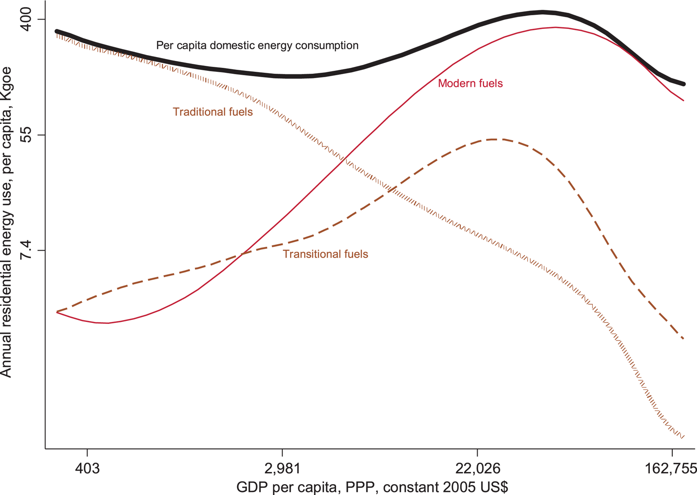
Figure 1 plots the relationship between energy consumption and per capita income, exploiting variability across countries and over time. The figure provides a historical view of patterns in domestic energy use over the world income distribution, showing how energy consumption (the bold line) tends to follow a nonlinear path depicted as a compressed S-curve. This shape seems to be explained by a marked shift in the composition of energy use. Energy consumption tends to be high at lower income levels, where the use of traditional fuels is prevalent. Moving to the right of the income distribution, traditional fuels are substituted with transitional and modern fuels. However, the use of transitional fuels tends to rise to a point from which it then starts to decline for further income increases. In contrast, consumption of modern energy grows nonlinearly until it accounts for most of the per capita consumption at the highest income levels. That is, as countries become wealthier, growth in overall per capita energy use tends to be explained mainly by larger consumption of better quality and more efficient fuels. Noticeably, this transition seems not to completely displace the use of traditional and transitional fuels in developed economies, a practice that may be attributed to cultural factors, or to consumption by low-income households within relatively rich countries.
Consumption of domestic fuels along the world income distribution.
Notes: Axes in log scale. The curves are fitted with a 2-degree polynomial for observations of 104 countries over 1971–2013. Modern fuels = electricity and gas; transitional fuels = kerosene, paraffin, and so forth; and traditional fuels = biomass. GDP, gross domestic product; Kgoe, kilograms of oil equivalent; PPP, purchasing power parity.
Source: Authors' calculations based on data from the International Energy Agency.

It is important to highlight that while in some developing countries the levels of total final energy consumption are high and even close to that of developed economies, their contexts are different. Not only is the quality energy mix dramatically different but so are the technologies that are used or accessible. For example, electricity provides greater efficiency for lighting than biomass, and access to more efficient light bulbs would increase this gap. Similarly, consumption of traditional fuels in developed countries would occur under very different circumstances, as for example, heating in better-off, isolated dwellings that use more efficient cook-stoves. All in all, this would imply considerable differences in the actual ‘useful energy’ enjoyed by the households.Footnote 6
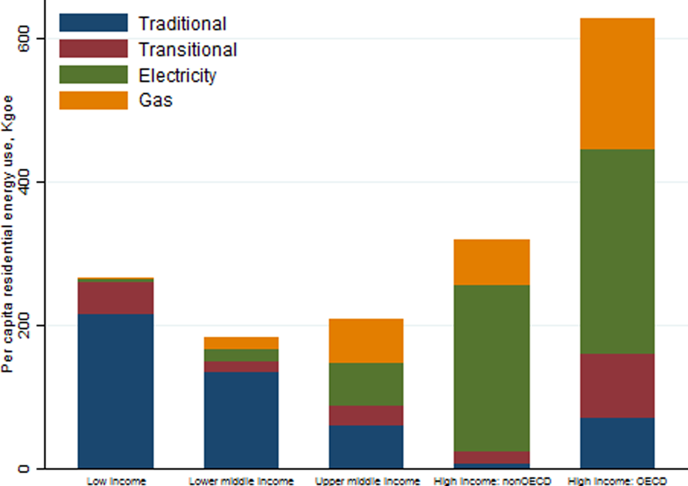
Beyond the expected differences in energy-quality and -efficiency, we observe systematic differences in the levels of energy consumption by income classification. This can be appreciated in figure 2 that presents the composition of annual per capita residential energy use, averaged over 2009–2013, by income group. It shows that total final energy consumption in high-income OECD countries is almost three times what is observed in the low-income group. Also, and in accordance with the above, this figure also shows that in low-income countries, traditional and transitional fuels represent 90 per cent of per capita energy consumption, a share that tends to sharply decrease with rising incomes.
Composition of per capita residential energy consumption by type of fuel and country income classification, average for 2009–13.
Notes: Countries are classified by their income level according to the World Bank income classifications. OECD: Organization for Economic Co-operation and Development; Kgoe: kilograms of oil equivalent.
Sources: Authors' calculations based on data from the International Energy Agency and World Development Indicators.

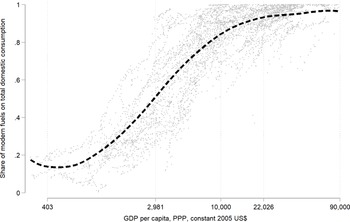
The resulting change in composition can be seen directly in figure 3, where the trend line of the share of modern fuels in domestic consumption follows a sigmoid shape –the gray dots are the scatter of the country-year observations. This reinforces the fact that modern fuels tend to displace other energy sources at the highest income levels. The switch toward modern fuels accelerates as countries develop, but the pace of substitution starts to decrease at higher-middle-income levels ($\mathrm{\ \mathbin{\lower.3ex\hbox{$\buildrel\succ\over {\smash{\scriptstyle\sim}\vphantom{_x}}$}}\ }$ US$10,000 per year). Still, a persistence of traditional and transitional fuels in the residential energy portfolio is observed. Such a slower pace may also be related to the last-mile problem, in which the difficulty of reaching isolated rural areas is an obstacle to achieving complete access to modern fuels.Footnote 7 On the other hand, the persistence of traditional and transitional fuels may also be the result of an optimal allocation by households, conditional on their preferences, resource availability, etc.
Share of modern fuels along the world income distribution.
Notes: The axes are in log scale. Values are for 104 countries between 1971 and 2013. Modern fuels include electricity and gas. The curve is fitted with a 2nd-degree polynomial. GDP, gross domestic product; PPP, purchasing power parity.
Sources: Authors' calculations based on data from the International Energy Agency and World Development Indicators.

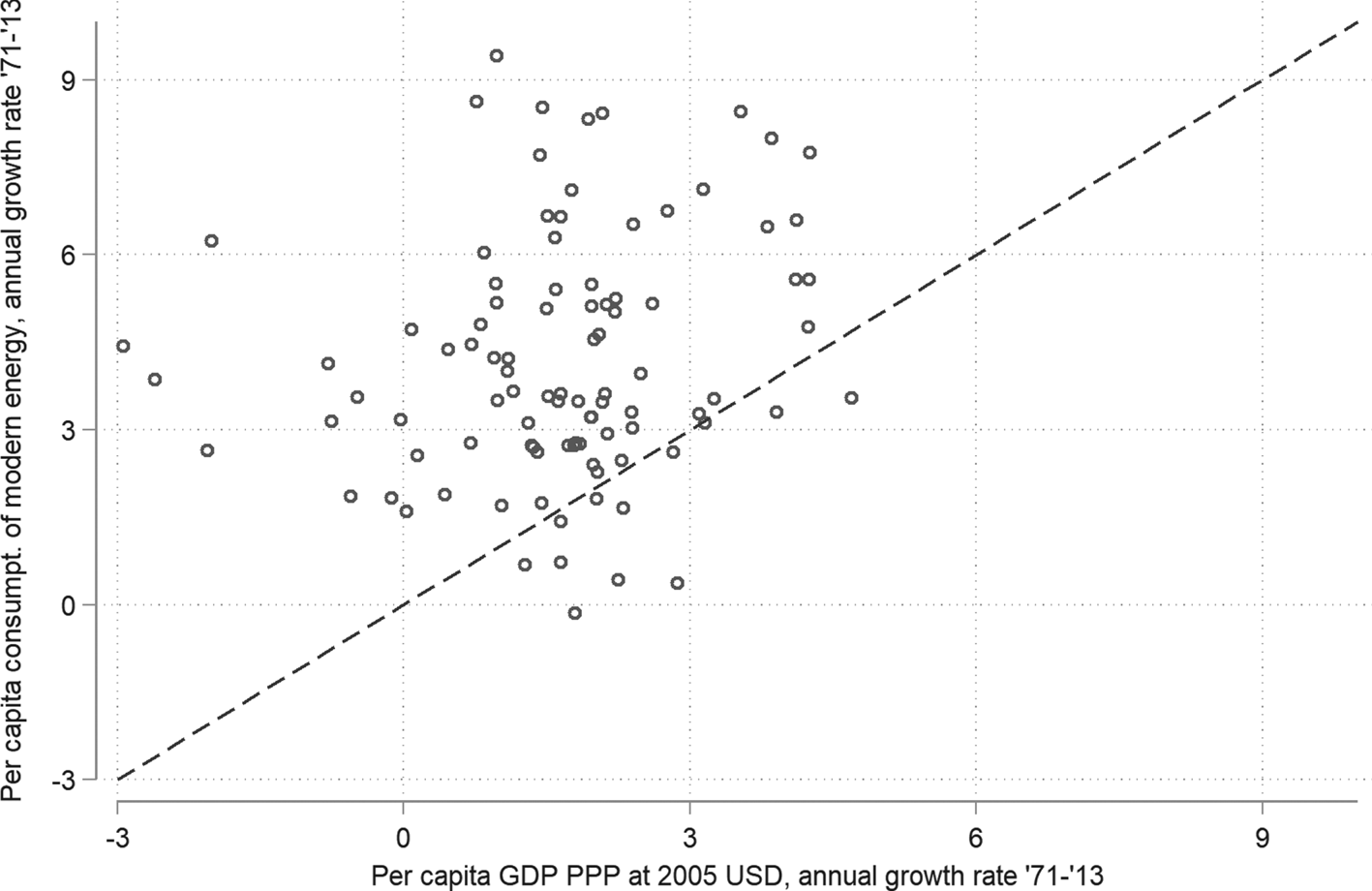
As inferred from the dispersion in the country-year observations, figure 3 also shows a pronounced heterogeneity in the energy transition paths. Such distinctive paths between countries can also be observed in terms of the relationship between the growth rates of modern energy consumption and GDP per capita. Figure 4 plots this relationship showing that it has been quite sparse, but also indicating that modern energy consumption has grown at a faster rate than income. This suggests that the estimation of income elasticities needs to take into account country-specific characteristics.
Modern energy consumption versus income growth.
Notes: Values are for 104 countries from 1971 to 2013. GDP, gross domestic product; PPP, purchasing power parity.
Sources: Authors' calculations based on data from the International Energy Agency and World Development Indicators.

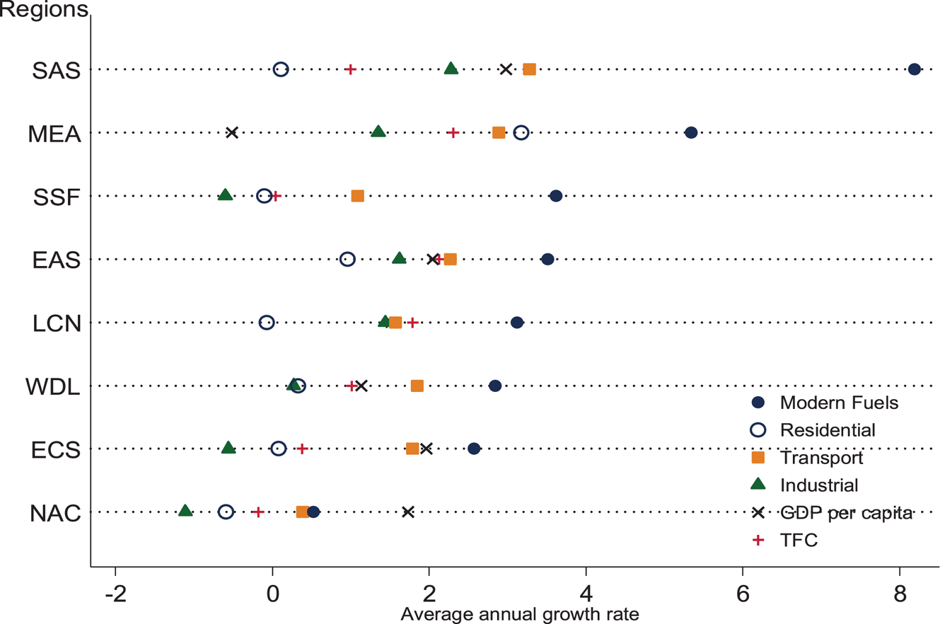
In a broader context, considering other economic sectors, residential modern energy consumption has not only grown at a higher rate than income but also at a higher rate than energy consumption by other sectors. Figure 5 illustrates that while per capita energy consumption in the residential sector has grown at relatively low rates in most regions, the modern fuel component has in fact grown faster than in other sectors, such as transportation and industry.Footnote 8 This pattern occurs in all regions, and it is especially marked in Sub-Saharan Africa, and the Middle East and North Africa.
Average annual growth rate by fuel, sector, and region.
Notes: Values are average annual growth from 1971 to 2013. Modern fuels = electricity and gas; transitional fuels = kerosene, paraffin, and so forth; and traditional fuels = biomass. Regions follow the World Bank classification: SAS, South Asia; MEA, Middle East and North Africa; SSF, Sub-Saharan Africa; EAS, East Asia and Pacific; LCN, Latin America and the Caribbean; WDL, world; ECS, Europe and Central Asia; and NAC, North America; GDP, gross domestic product; TFC, total final consumption of all sectors. GDP per capita is in constant 2005 PPP prices.
Source: Authors' calculations based on data from the International Energy Agency and World Development Indicators.

4. Empirical approach
The composition and sensitivity of domestic energy consumption are examined using parametric and machine-learning approaches. In the parametric setting, the general specification takes the following reduced forms:


where ${y_{it}}$ represents a dependent variable for country i in year t. The dependent variables are (separately) consumption of traditional, transitional, modern fuels, and the share of modern fuels, all measured in per capita terms. The share of modern fuels aims to capture the composition of domestic energy consumption, which is calculated as $s = m/E$
 , the ratio of modern fuels $(m)$
 in total residential energy consumption $(E)$
 , and therefore is defined within the range $[{0,1} ]$
 . The main independent variable is per capita income $({x_{it}})$
 , with $\alpha$
 the vector of parameters of interest.
The set of covariates, ${W_{it}}$ , includes international petroleum prices, the share of power produced from hydro, net exports of fossil fuels, country-specific dummies and/or country-specific trends (for the MG and CCE estimators). This specification does not control for end-user energy prices (electricity and gas) for the entire sample. Since our main interest is estimating $\alpha$
 , we expect that the set of the other covariates captures differences in energy prices; for example, oil prices may be relevant in countries with a low natural capital endowment, while hydro participation and net exports of fossil fuels may help to account for differences in other cases. Besides, we expect that the country-specific trends will account for the absence of energy prices, among other time-variant unobservables (such as temperature and urbanization trends). Nonetheless, in a robustness check, we replicate the main results including electricity prices instead of oil prices.
We apply the following estimators: (i) the fixed effect (FE) estimator, which is the standard baseline and it is expected to perform well in the dynamic setting under samples with large T and N,Footnote 9 which is the case herein, since we restrict the sample to those countries with the longest time series. This estimator allows cross-country heterogeneity that is fixed over time, but assumes coefficient homogeneity and cross-sectional independence; (ii) the Pesaran and Smith (Reference Pesaran and Smith1995) mean group estimator (MG), which takes into account time-variant unobservables for each country and coefficient heterogeneity, while still assuming cross-sectional independence; and (iii) the Pesaran (Reference Pesaran2006) Common Correlated Effects (CCE) estimator, which further allows cross-sectional dependence (CSD), requiring only covariates with cross-sectional variation. The CCE model, therefore, does not include international oil prices.Footnote 10 Although a less restricted specification and estimator would be preferable, it is also interesting to evaluate the differences between these estimators. Also, the time variant unobservables in the MG and CCE estimators, would help to capture, among others, the effect of the technological and structural change.
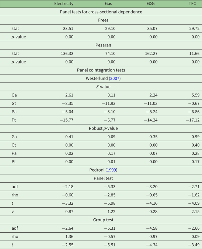
The panel analysis requires examination of the properties of the series. Table 1 summarizes two characteristics of the series: cross-sectional dependence and cointegration. According to the Frees and Pesaran tests, the residuals of equation (1) present nonconstant variance and cross-sectional dependence, supporting the use of the CCE estimator. Regarding cointegration, two types of cointegration tests are applied: those proposed by Pedroni (Reference Pedroni1999) and those proposed by Westerlund (Reference Westerlund2007). Both types of tests are estimated with no intercept and no deterministic trends, and the optimal lags are determined using the Akaike information criterion.
CSD and cointegration tests for domestic fuels

Notes: E&G, electricity and gas; CSD, cross-sectional dependence; TFC, total final consumption of the residential sector; a, semiparametric test; adf, Augmented Dickey–Fuller test; G, group mean test; P, panel test; t, parametric test.
All CSD tests were performed after FE regressions. The null hypothesis is cross-sectional independence. The robust p-value is for a one-sided test based on a bootstrapped distribution (500 bootstrap replications). The Westerlund tests are applied with no intercept, no deterministic trends, and the optimal lags are determined using the Akaike information criterion.
Table 1 shows that both groups of tests return similar results for electricity, gas, and modern fuels, for LAC and all countries, suggesting a stable long-run relationship between income and modern residential energy sources. However, the results are less conclusive for the case of total final consumption (TFC) by the residential sector, specifically in the case of the Westerlund tests. Recall that in the tests proposed by Westerlund (Reference Westerlund2007), the null hypothesis (Ho) of no cointegration is evaluated for nonstationary cases with heterogeneous dynamics.Footnote 11 The group-mean test (G) rejects the Ho if at least one country there is cointegration, while the panel tests (P) reject the Ho if there is cointegration for the panel as a whole. The Westerlund tests are applied to the main variables under analysis; moderns fuels and TFC as dependents, and income per capita as independent. The panel tests and the group mean parametric test tend to not accept Ho for electricity, gas, and modern fuels, suggesting a stable long-run relationship between income and modern residential energy sources. The null cannot be rejected in the case of group mean semi parametric test (Ga), and for any test, in the case of the TFC of the residential sector.
With respect to the proposed specification, the energy consumption, income, and price variables are expressed in logarithmic, so the estimates from equation (1) can be interpreted as short-run elasticities. However, a relevant distinction is the long-run effect of income changes on energy consumption and its composition. The long-run relationship is captured by including the lagged dependent variable as a regressor in equation (2) and then calculating the long-run elasticity as the corresponding derivative, which in a linear setting is ${\varepsilon _{E,x}} = \alpha /({1 - \theta } )$ , where $\theta$
 is the coefficient of the lagged variable.
These regressions return average elasticities which are informative by type of fuel but not for the suspected changing association between income and energy consumption along the income distribution. To address this issue, the regressions are also performed by income group, which allows for the evaluation of the change in income elasticities across groups at different development stages at the cost of reducing the sample per estimation and not accounting for changes in the sample composition (i.e., countries that may move from one income classification to another).
To further examine the change in consumption of modern fuels, we replace the linear income regressor with an income polynomial, with its degree being chosen based on cross-validation procedures.Footnote 12 In a linear setting, $\alpha$ is expected to be positive, while a polynomial can capture potential nonlinearities, approximating the shape of the responsiveness to income changes. From a conceptual viewpoint, in a nonlinear setting, the sign and significance of $\alpha$
 are less clear but may have relevant implications for capturing how energy consumption patterns change along the income distribution. Notice that this framework still assumes a functional form and constant parameters for each country.
The next step is to completely relax the functional form and to allow for complete heterogeneity of the income elasticity along the world income distribution. This problem is quite complicated in semiparametric or nonparametric settings, where the returned coefficients are difficult to recover and interpret. An efficient approach for discovering patterns, when the correct functional form is unknown, is the application of machine-learning methods. In particular, a flexible and interpretable method, described by Hainmueller and Hazlett (Reference Hainmueller and Hazlett2014), is the Kernel Regularized Least Squares (KRLS), which allows estimation of the full distribution of $\alpha$ without relying on parametric assumptions such as linearity or additivity. The KRLS estimator states and solves the following problem:Footnote 13

where ${\omega ^\ast }$ = test point coefficients or weights, containing $\alpha$
 and $\beta$
 ; y = outcome variable; and K = matrix of kernel functions $({{z_j},{z_i}} )$
 where z represents the vector of covariates, previously defined as x and W.
In equation (3), the loss function takes the least-squares form using the Gaussian kernel function K. The kernel function, $k(. )$ , measures the similarity between observations for each ${z_i}$
 . A greater similarity translates to a greater influence of ${z_i}$
 over the outcome. Therefore, $K\omega$
 represents a space of functions that aim to approximate the outcome point to point, such that similar observations would tend to have similar outcomes. λ weights the complexity of the function, such that greater values represent larger penalties for complexity.Footnote 14
This problem is solved computationally, and the search for the best fit of the KRLS does not impose any functional parametric form, such that it does not assume constant marginal effects. That is, the estimated vector $\alpha$ contains the pointwise income elasticities by country at each point of the income distribution. This is important in our context as the returned distribution of coefficients will display long-run information without requiring transformation. However, and in contrast with the MG and CCE estimators, such pointwise estimates can be interpreted in local terms as reflecting the structural conditions and available technology (and technology adoption) in each point of the income distribution.Footnote 15
In line with the above, an important aspect of the empirical analysis is determining whether the estimates have a causal interpretation or represent conditional correlations. It is expected that the inclusion of the covariates and fixed effects helps to clean the relationship between energy and income of omitted factors. However, potential econometric problems are not being addressed, such as income endogeneity or measurement error. Therefore, since there is a conceptual and empirical basis to argue for bi-directionality between income and consumption of modern energy sources, we attach no causal interpretation to the estimates.
5. Results
5.1 Panel estimates
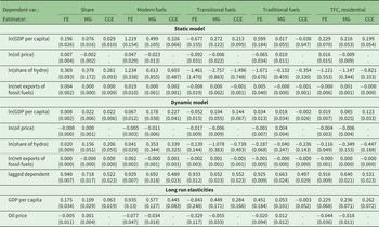
The panel regressions are summarized in table 2 showing significant differences by estimation method. With the exception of residential TFC, the FE estimator tends to return stronger associations with income per capita, while accounting for country-specific trends (MG) and cross-sectional dependence (CCE) systematically reduces the estimated elasticities.
Elasticities for domestic energy consumption

Notes: Robust standard errors in parentheses. FE, fixed effect; MG, mean group; CCE, common correlated effects; TFC, total final consumption The static model, equation (1), shows the short-run elasticities. Long-run elasticities are derived from the dynamic model, equation (2), and their corresponding standard errors are estimated using the delta method. In the case of share of modern energy, the elasticity is calculated at the fuel sample average of $s$ (0.72). MG and CCE include country-specific trends. CCE corrects for cross-sectional correlation.
A common pattern between estimators is that modern fuels are more sensitive to income than total residential energy consumption, which we interpret as a result of the nonlinear pattern originating from the observed change in fuel composition. This compositional change is supported by the strong association between the share of modern fuels and income in the short and long run. Still, in the case of non-modern fuels, the panel estimations present higher variance. The income elasticities for transitional fuels present a wider range of variation across estimators from −0.84 (FE) to 0.45 (MG), with the preferred model returning 0.28 (CCE), statistically significant in all cases. In the case of traditional fuels, income elasticities tend to be negative but not statistically significant.
As expected, long-run elasticities tend to be greater than short-run elasticities for modern fuels, suggesting an adaptive response by households. On average, a 1 per cent increase in income translates into a 0.33 per cent increase in modern fuel consumption in the short run, and a 0.44 per cent increase in the long run (under the CCE model).
Overall, these estimates are aligned with both energy consumption hypotheses, suggesting a greater substitution effect for traditional fuels, and a positive wealth effect over transitional and modern fuels. This supports the intuition that modern domestic fuels exhibit characteristics of normal goods, whereas traditional fuels exhibit characteristics of inferior goods, implying that households attach a substantial positive value to the benefits and convenience of using modern fuels.
5.2 Elasticities by income level
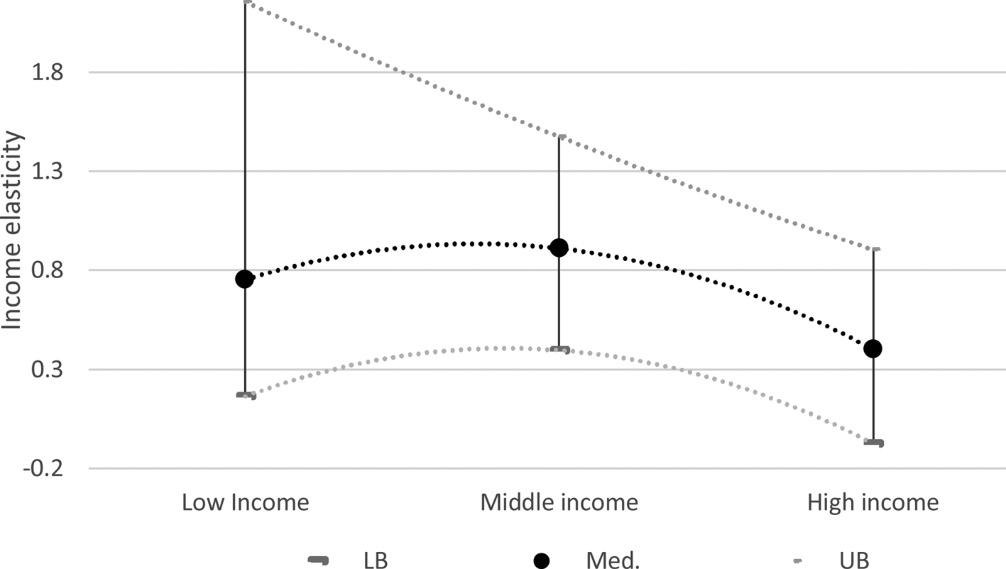
This section explores whether the energy income elasticities are constant along the income distribution, that is, if energy consumption increases at a constant rate independent of income level. Figure 6 presents bands of elasticities by income group, where the lower (LB), median (Med), and upper (UB) points are, respectively, the minimum, median, and maximum of the set of estimations returned under the FE, MG or CCE models. Table A2 (online appendix) presents the regression results. The results suggest that elasticities decrease as countries grow wealthier, but with a great degree of heterogeneity within each income group. At the highest income level, the elasticity range includes negative values, indicating that for some countries income increments have led to reductions in their per capita domestic consumption. This result supports the concavity observed in figure 1.
Estimator band of long-run income elasticity of modern fuels by income classification.
Notes: The lower (LB), median (Med.), and upper (UB) bands are the minimum, median, and maximum of the set of estimation methods (FE, MG, CCE) in each income group. Countries are grouped into low, middle, and high income according to the World Bank income classification. Regression results are presented in table A2 in the online appendix.

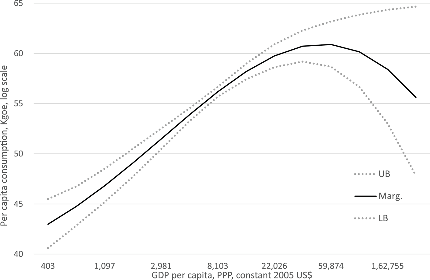
To provide a view of how the elasticities translate into per capita energy consumption, figure 7 shows the estimated income effect on modern energy use. For simplicity, it uses the FE estimator with an income polynomial. This specification provides flexibility in analyzing the relationship between energy and income, allowing for potential nonlinearities. In the case of modern fuels, the best fit was based on cross-validation procedures and was found to be a third-degree polynomial (see table A1, online appendix).Footnote 16 The estimates resemble a concave curve, indicating that energy consumption would grow at a decreasing rate as a country's income level rises.Footnote 17 That is, the income elasticity of energy demand would be negative at some point to the right of the global income distribution, consistent with the negative elasticities estimated toward the lower band of figure 6.
Long-run estimated income effects of modern energy consumption.
Notes: GDP: gross domestic product; Kgoe: kilograms of oil equivalent. Scales are in logs. The estimation is based on 104 countries. In-sample predictions. The specification accounts for country specific trends. The predicted margins are implemented with the best fit third-degree polynomial for GDP per capita. The model was selected on the basis of adjusted R 2, RMSE, BIC, and AIC where RMSE, root mean square error; BIC, Bayesian information criterion; AIC, Akaike information criterion.

These patterns indicate a strong energy dependence for accompanying economic growth which only starts to decrease at high levels of economic development. At the same time, the simulated reductions in energy consumption, in the residential sector, are consistent with recent trends in energy consumption observed in the United States and OECD countries (BP, 2016). It should noted that reductions in per capita energy use, in these estimations, only occur at extremely high-income levels, however, the overall simulated trend is consistent with stylized facts reported in the literature. For example, for the case of overall per capita energy consumption, van Benthem and Romani (Reference van Benthem and Romani2009) and Medloock and Soligo (Reference Medlock and Soligo2001) show similar concavities for income elasticity and energy use over the income distribution, respectively. More recently, Csereklyei et al. (Reference Csereklyei, Rubio-Varas and Stern2016) show that while some decoupling between per capita energy use and income has occurred, it is still insufficient to offset the growing energy demand. Our estimates add evidence for the residential sector, with greater detail regarding the composition of its energy portfolio.
It is also worth mentioning that it is unclear what the roots of the concavity may be. Two potential explanations are the existence of satiation points in energy consumption for households and/or net energy efficiency gains that seem to be more pronounced at high-income levels. In the case of the United Kingdom, Fouquet (Reference Fouquet2014) argues that while energy efficiency improvements may have a significant rebound effect at middle-income levels, at higher levels, those improvements translate into net energy savings, explaining, to some extent, the reduction in income elasticities for modern fuels.Footnote 18
5.3 Distribution of elasticities – KRLS results
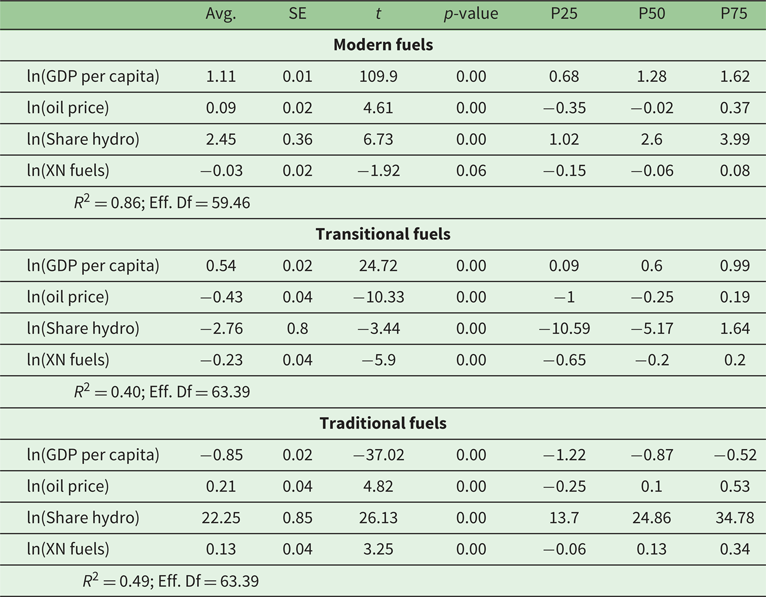
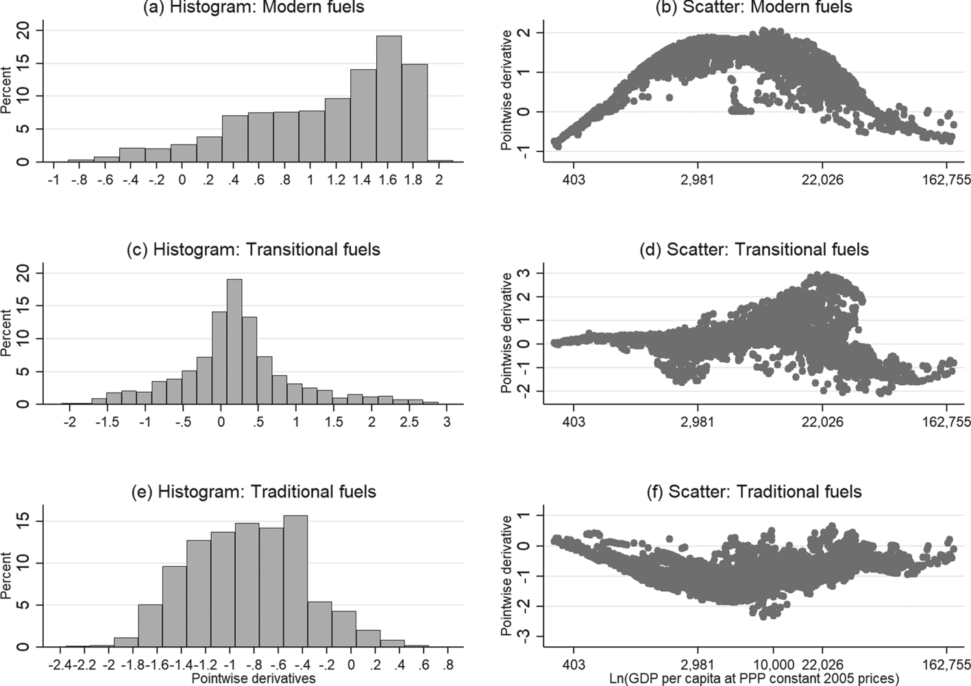
Table 3 reports the results from the KRLS estimator by fuel type, corroborating a marked coefficient heterogeneity. In the case of modern fuels, the distribution of the income coefficients ranges from 0.68 in the 25th percentile to 1.62 in the 75th percentile. Interestingly, these coefficients tend to be greater than the estimation in the parametric setting, emphasizing the relevance of income when arranging the domestic energy portfolio, once complete heterogeneity is allowed and the functional forms are relaxed. Figure 8(a) presents a histogram of the income coefficients, showing that the distribution is left-skewed with over 60 per cent of the density concentrated between 1.0 and 1.8, explaining the high average values of $\hat{\alpha }$ .
KRLS pointwise derivatives

Notes: Avg., average coefficient; SE, standard error; XN, net exports.
Estimated income pointwise derivatives along the income distribution.
Note: In the distribution graphs, the x-axes are in log scales.

However, the estimated distribution of the income elasticity for modern energy carriers is consistent across parametric and non-parametric approaches. The scatters in figure 8 indicate that the observed heterogeneity is greatly shaped by the stage of economic development (following indications in figures 6 and 7). Further, conditional on the income level, the distribution of $\hat{\alpha }$ – the income elasticity of modern energy consumption – shows an inverse U-shape; the sensitivity to income increases up to a maximum of around 2 for income levels between US$8,500–9,500 per capita, and then decreases as income continues to rise (see figure 8(b)). The concentration at high values of $\hat{\alpha }$
 is mainly explained because of our sample composition with more than 50 per cent of countries belonging to lower-middle and upper-middle income groups. In these stages, we tend to observe the greater association between income and energy consumption. In general, this pattern is consistent with previous results, in the sense that the higher the development stage of a country, the less sensitive residential demand for modern energy would be to further income changes.
Overall, these results are also consistent with previous findings showing that energy intensity and income elasticity increase with income up to a peak from which it starts to decline (see Galli, Reference Galli1998; Fouquet, Reference Fouquet2014; Van Benthem, Reference van Benthem2015). For a sample of 10 Asian economies between 1973–1990, Galli (Reference Galli1998) shows a non-monotonic relationship between income and energy intensity, indicating that the latter increases with income in low-income economies, but decreases (with income) in high-income economies (although the per capita income turning point can vary widely by economy, ranging from 758 to 7,659 in PPP$1985). Using two centuries of time series from the United Kingdom, Fouquet (Reference Fouquet2014) shows income elasticities for energy services that follow an inverse U-shaped curve across phases of economic development. A similar pattern is found for a sample of 76 countries by Van Benthem (Reference van Benthem2015), suggesting a turning point at around a GDP per capita of $10,000 (US$ 2000, PPP).
Further, the observed negative income elasticities at the highest income levels are consistent with the recent trends in OECD high-income countries, where residential per capita energy use has recently registered reductions (BP, 2016). Although not statistically significant, Van Benthem (Reference van Benthem2015) find negative income elasticity for income levels between $20,000–30,000 (US$ 2000, PPP).
The results for transitional and traditional fuels are also consistent with previous estimations, and with the energy consumption hypotheses. Notice that on average, the relationship between income and consumption of traditional and transitional fuels is statistically stronger than in the panel regressions (see table 3). Regarding the pointwise estimates, we observe that the income sensitivity of transitional fuels exhibits an inverse U-shape along the income path. At early stages of economic development, transitional fuel consumption tends to respond positively to income changes; however, after reaching relatively high-income levels, the income elasticity becomes negative, indicating a reduction in consumption. Along the same lines, traditional fuels are concentrated at negative values. In comparison with the elasticities in table 2, these results offer greater clarity on the association between income and domestic energy consumption.
The other covariates are, on average, statistically significant as well; however, their distributions are difficult to interpret (see table 3). In the online appendix, figure A1 presents histograms of the price coefficient by type of fuel. In the case of modern fuels, the coefficient for oil prices is negative and symmetrically distributed at the median. On average, it is positive and quite small, at less than 0.1 per cent. In the case of transitional fuels, which are mainly oil products, the price elasticity is significantly negative, but with bi-modal distribution; one mode around −1 and the other around 0. In the case of traditional fuels, the estimated price elasticity is positive. This is expected since oil prices may be interpreted as proxies for substitute energy sources. However, as international oil prices are not an accurate measure of energy prices, these results should be interpreted with caution. Moreover, well-behaved price elasticities for energy demand have been elusive in the empirical literature, particularly in applications with aggregated data (Dahl and Sterner, Reference Dahl and Sterner1991; Fouquet, Reference Fouquet2014).
5.4 Robustness check
To evaluate if previous results are severely distorted by the absence of energy prices in each country, we perform the main regressions of sub-sections 5.1–5.3 but including electricity prices instead of international oil prices. We decided to use electricity prices – rather than, for example, natural gas prices – as they are available for more countries, while natural gas is generally less used in the Latin American Region. This exercise focuses on the share and the consumption of modern fuels. The results are available in online appendix table A3.
Concerning the panel-estimations, the derived income elasticities are statistically similar to those presented in table 2, for modern energy share and consumption (as the confidence intervals of the income elasticities overlap). The price elasticities continue to be statistically not significant. The in-sample prediction of modern energy consumption shown in the online appendix (figure A2) returns higher levels of per capita consumption, however, its shape, over the income distribution, resembles those of figure 7 also indicating decreasing income effects at advanced stages of economic development. On the other hand, the estimated KRLS coefficients, online appendix figure A3 and table A4, seem to correspond to the right side of the distribution in figure 8, which is consistent with the income levels in this sub-sample (for which there is available electricity prices data). Overall, these estimates suggest that our results and specifications are robust to the inclusion of alternative energy prices.
In addition, as suggested by referees, the online appendix presents two robustness exercises: the Bias Corrected FE or Kiviet estimator (Judson and Owen, Reference Judson and Owen1999; Galiani and Gonzalez-Rozada, Reference Galiani and Gonzalez-Rozada2002), and the Arellano & Bond estimator. The results in online appendix table A5 are consistent in terms of sign and statistical significance. While the size of the coefficients varies across dependent variables and estimators, the implied elasticities are similar to the FE estimator presented in table 2. In the case of transitional and traditional energies, they continue to be not statistically significant. The additional estimations also show that bias-corrected FE returns (when statistically significant) lower coefficients, which appears to be aligned with our MG and CCE estimates in table 2.
6. Conclusions
In addition to energy consumption rising with income, its composition also shifts toward greater use of modern and more efficient fuels. Over the past four decades, this empirical fact has been observed in the residential sector, where demand for electricity and gas has grown at higher rates than in the transport and industry sectors, replacing demand for dirtier energy carriers. In this process, the income elasticity of residential energy demand has evolved, forming an inverse U-shape along the world income distribution. This pattern prevails to different specifications and estimation methods. This result may be suggesting that household energy use may reach a satiation point beyond which net energy savings will begin to reduce per capita residential energy use at high levels of economic development.
This paper also highlights the importance of taking country heterogeneity into account, as well as distinguishing between energy sources when analyzing the relationship between income and energy use. Our results suggest that income elasticity follows consistent patterns across development stages, in which economic growth is mainly related to greater consumption of modern energy sources, rather than traditional or transitional ones. Along this path, traditional fuel behaves as an inferior good, implying that households attach significant value to the benefits and convenience of switching to modern fuels. However, the results also show variability between countries even at equivalent income levels and same type of energy carrier. That is, the association between consumption of energy carriers and economic growth can vary and be subject to country circumstances, being relevant for energy planning.
By focusing on the residential energy portfolio and using parametric and machine learning approaches, the findings of this paper complement the literature studying the energy-income relationship. Our results are consistent with previous studies emphasizing the increasing energy demands of the developing world. Further, the analysis provides empirical insights on the dimension of the policy challenges aimed at reaching a cleaner economic growth path. Indeed, ascending the development ladder has been strongly linked with incremental demands of electricity and gas, while the use of transitional fuels remains substantial in developed countries and net energy savings seems to have an aggregate impact only at the highest income levels. That is, the carbon content of household energy consumption remains significant even at most developed economic stages. Therefore, it seems apparent that economic progress has not been necessarily accompanied by a sustainable energy portfolio. In this context, relevant research avenues are those addressing the effectiveness of energy and environmental policies to decarbonize the household energy services porfolio and to accelerate the materialization of energy savings in an affordable way.
Supplementary material
The supplementary material for this article can be found at https://doi.org/10.1017/S1355770X22000067.
Acknowledgements
A previous version was published as a Working Paper at the Inter-American Development Bank. The findings, interpretations, and conclusions herein are strictly those of the authors and should not be attributed in any manner to their affiliated institutions. This version has benefited from comments and suggestions from Andrea Guerrero, Daniel Hernaiz, Namho Kim, and two anonymous peer reviewers. All remaining errors are our own responsibility.