In social science research, it is common to confront data that are clustered or grouped into higher-level units. One of the most frequently encountered challenges when modeling these data arises when the dependent variable exhibits group-level variation beyond what can be explained by the independent variables alone. In these cases, fitting a standard linear regression or generalized linear model without accounting for the grouped nature of the observations can lead to poorly fitting models and misleading estimates of both the effect of independent variables of interest and of the precision of those estimates (Beck and Katz Reference Beck and Katz1995; Greene Reference Greene2012).
The two dominant approaches to remedy this problem are the use of so-called fixed-effects or random-effects models.Footnote 1 Although much has been written on the theoretical properties of both approaches (for example, Kreft and DeLeeuw Reference Kreft and de DeLeeuw1998; Robinson Reference Robinson1998; Kennedy Reference Kennedy2003; Frees Reference Frees2004; Gelman Reference Gelman2005; Wilson and Butler Reference Wilson and Butler2007; Arceneaux and Nickerson Reference Arceneaux and Nickerson2009; Wooldridge Reference Wooldridge2010; Greene Reference Greene2012), recommendations for applied researchers are often confusing—or even contradictory (Gelman and Hill Reference Gelman and Hill2007, 245). Often they are made with reference to idealized datasets with very large sample sizes, or using divergent standards for assessing model quality. There remains little consistent guidance for researchers trying to decide how best to model the data they have on hand. They are left to wonder: “Should I use fixed or random effects?”
In this article, we offer practical guidance for researchers choosing between fixed- and random-effects models. As we describe below, both models entail a series of assumptions that might be violated in any given dataset. Under certain conditions, random effects models can introduce bias, but reduce the variance of estimates of coefficients of interest. Fixed-effects estimates will be unbiased, but may be subject to high sample dependence. We argue that researchers ought not to place undue weight on minimizing either bias or variance, but rather consider the trade-off between the two in either model. While it is true that under a random-effects specification there may be bias in the coefficient estimates if the covariates are correlated with the unit effects, it does not follow that any correlation between the covariates and the unit effects implies that fixed effects should be preferred. What should be judged instead is how much bias is created, and how much variance would be introduced by using fixed effects instead. After all, except in exceptional circumstances, there will always be some level of correlation between the covariates and the unit effects, and thus at least minimal bias (for example, Angrist and Pischke Reference Angrist and Pischke2009, 223n2). The question is, how much is too much?
We compare the performance of the fixed- and random-effects models using a series of Monte Carlo experiments that vary the sample size, effect size of the independent variable, correlation between the independent variable and unit effects, and, crucially, whether the majority of variation in the dependent variable is within or between units. We then calculate how consistently each model recovers the true coefficient of interest. Drawing upon our simulation results, we derive a set of guidelines that applied researchers can use to determine how best to specify models for grouped dependent variables.
The Problem
We consider the linear model for observations i=1 … N grouped into units j=1 … J,
 $$y_{i} =\alpha _{{j[i]}} {+} \beta x_{i} {+}{\varepsilon}_{i} ;\,\quad \quad {\varepsilon}_{i} \!\sim \!N(0,\sigma _{y}^{2} ).$$
The effect of x on y, denoted β, is the primary quantity of interest. We assume that β is the same within each unit.Footnote 2 However, even after accounting for the effect of x, there may still remain additional variation in the overall level of y across units. The unit effect α j captures the amount by which predictions of y in unit j must be adjusted upward or downward, given knowledge only of x. The notation j[i] indicates the unit j of observation i.
One interpretation of the unit effects is that they represent ignorance about all of the other systematic factors that predict y, other than x. If these factors were known, they could ostensibly be included as additional covariates in the model, thus “explaining” the extra variation in y and eliminating variation in α j across units. Since these variables are not included in the model, we capture their effects with α j instead. The variation in α j might also be partially or completely nonsystematic, due simply to stochastic noise.
With few exceptions, failing to allow for the possibility that α j varies by unit will lead to biased estimates of β. If we assume that the unit effects are all equivalent—that is, α j =α k for all j and k —then Equation 1 reduces to the pooled model
 $$y_{i} =\alpha \, {+}\, \beta x_{i} \, {+}\, {\varepsilon}_{i} ;\quad \quad {\varepsilon}_{i} \sim N(0,\sigma _{y}^{2} ).$$
The pooled regression model is appropriate if α j does not vary once x is included as an independent variable. The pooled model will also not produce bias in estimates of β if the unit effects differ but are uncorrelated with x. In most applications, however, the unit effects are associated to some degree with x, so variation in α j must be modeled in order to avoid faulty inferences about β.
Two Solutions: Fixed and Random Effects
There are two standard approaches for modeling variation in α j : fixed effects and random effects. The fixed-effects model is a linear regression of y on x, which adds to the specification a series of indicator variables z j for each unit, such that z j[i]=1 if observation i is in unit j, and z j[i]=0 otherwise:
 $$y_{i} =\mathop{\sum}\limits_{j=1}^J \alpha _{j} z_{{j[i]}} \, {+}\, \beta x_{i} \, {+}\, {\varepsilon}_{i} ;\quad \quad {\varepsilon}_{i} \! \sim \!N(0,\sigma _{y}^{2} ).$$
The coefficients
 $$\hat{\alpha }_{j} $$
that are computed for each z
j
are taken as estimates of α
j
.
In the random-effects model, the α
j
are instead assumed to follow a probability distribution, with
parameters estimated from the data. This distribution is typically normal, with
average unit effect μ
α
and variance
 $$\sigma _{\alpha }^{2} $$
, which describes by how much the other unit effects vary
around the mean.
 $$y_{i} =\alpha _{{j[i]}} \, {+}\, \beta x_{i} \, {+}\, {\varepsilon}_{i} ;\quad \quad \alpha _{j} \! \sim \!N(\mu _{\alpha } ,\sigma _{\alpha }^{2} );\quad \quad {\varepsilon}_{i} \! \sim \!N(0,\sigma _{y}^{2} ).$$
As Gelman and Hill (Reference Gelman and Hill2007, 258) note, the random-effects estimator is equivalent to the
fixed-effects estimator when we assume that α
j
∼N(μ
α
,∞) rather than
 $$\alpha _{j} \! \sim \!N(\mu _{\alpha } ,\sigma _{\alpha }^{2} )$$
.
The estimators of the coefficient β under the two models are mathematically related. Let x j and y j represent the n observations in the jth unit. Following Greene (Reference Greene2012, 373), the generalized least squares estimator of β for the random-effects model is:
 $$\hat{\beta }_{{RE}} =\left( {\mathop{\sum}\limits_{j=1}^J {\bf x}{\rm '}_{j} Σ^{{{−}1}} {\bf x}_{j} } \right)^{{{−}1}} \left( {\mathop{\sum}\limits_{j=1}^J {\bf x}{\rm '}_{j} Σ^{{{−}1}} {\bf y}_{j} } \right),$$
where, letting I be the n×n identity matrix and i be an n×1 column of ones,
 $$Σ^{{{−}1/2}} ={1 \over {\sigma _{y} }}\left[ {{\bf I}{−}{\theta \over n}{\bf ii'}} \right]$$
with
 $$\theta =1{−}{{\sigma _{y} } \over {\sqrt {\sigma _{y}^{2} \, {+}\, n\sigma _{\alpha }^{2} } }}.$$
As
 $$\sigma _{\alpha }^{2} \to\infty$$
or n→∞, θ→1,
making the random-effects estimator
 $$\hat{\beta }_{{RE}} $$
reduce to the fixed-effects estimator
 $$\hat{\beta }_{{FE}} $$
(Greene Reference Greene2012,
361).
How to Choose?
In some cases, choosing between a fixed- and random-effects specification will follow directly from a researcher’s theoretical model. Or a researcher may have application-specific concerns about the appropriateness of the assumptions underlying either model. Unfortunately, however, too often one’s theoretical model does not dictate a particular specification, and the theoretical assumptions about which one might be concerned do not lend themselves to empirical evaluation. In these situations, neither specification emerges as an obvious choice. In this context, we investigate empirically which model offers better inferences about the quantities of interest. Both models have potential advantages—as well as disadvantages—to consider when selecting an approach.
The problem of high variance
The estimate of β in the fixed-effects model may, under certain conditions, produce estimates that are highly sample dependent—that is, overly sensitive to the random error in a given dataset. Suppose that there are few observations per unit, or that x varies little within each unit, relative to the amount of variation in y. Estimates of the within-unit effects of x on y may then diverge considerably from the true effect due to chance alone.Footnote 3 If there is also a small number of units, then many of the within-unit effects may diverge from the true effects in the same direction, leading the estimate of β to be quite different from the true β. This lack of robustness to potentially anomalous samples is what is meant by the fixed-effects model having high variance.
A related drawback of fixed-effects models is that they require the estimation of a parameter for each unit—the coefficient on the unit dummy variable. This can substantially reduce the model’s power and increase the standard errors of the coefficient estimates. The problem is worsened when the within-unit sample size is very small, as the unit effects alone may account for most of the variation in the dependent variable.
Random-effects models enable estimation of β with lower
sample-to-sample variability by partially pooling
information across units (Gelman and Hill Reference Gelman and Hill2007, 258). By estimating the variance parameter
 $$\sigma _{\alpha }^{2} $$
in Equation 4, the random-effects estimator forms a compromise between the
fixed-effects and pooled models. Groups with outlying unit effects will have
their respective α
j
shrunk back toward the mean, μ
α
. This brings estimates of β away from the less stable fixed-effects
estimate and closer to the more stable (albeit potentially biased) pooled
estimate. The effects of shrinkage will be greatest for units containing
fewer observations, especially when estimates of
 $$\sigma _{\alpha }^{2} $$
are close to zero.
The problem of bias
The most serious drawback of the random-effects approach is the problem of bias that partial pooling can introduce in estimates of β. To eliminate this bias, the random-effects estimator requires there to be no correlation between the covariate of interest, x, and the unit effects, α j . To illustrate, suppose that there is a variable z that predicts y but is not included as a covariate in the random-effects model. As a result of omitting z from the model specification, the higher or lower levels of y in unit j due to z are instead accounted for by the unit effects α j . For there to be no bias in estimates of the coefficient on x, there must be no correlation between x and z—and, hence, no correlation between x and α j , implying no confounding due to the omitted z. Since the random-effects model does not estimate separate unit effects, any correlation between x and α j can imply an omitted variable z that produces bias in estimates of β. The greater the magnitude of the correlation between x and α j , the greater the bias in estimates of β.Footnote 4
Scholars are sometimes advised to use a Hausman (Reference Hausman1978) specification test to detect violations of the random-effects modeling assumption that the explanatory variables are orthogonal to the unit effects. A “significant” test result is taken as evidence of a correlation between x and α j , implying that the random-effects model should be rejected in favor of the fixed-effects model. However in most applications, the true correlation between the covariates and unit effects is not exactly zero. Therefore, if the Hausman test fails to reject the null hypothesis of orthogonality, it is most likely not because the true correlation is zero—and, hence, that the random-effects estimator is unbiased. Rather, it is likely that the test has insufficient statistical power to reliably distinguish a small correlation from zero correlation. When using the random-effects model, there will still be bias (if perhaps negligible) in estimates of β, even if the Hausman test does not find a significant result. Of course, in many cases, a biased (random-effects) estimator can be preferable to an unbiased (fixed-effects) estimator if the former provides sufficient variance reduction over the latter. The Hausman test does not help evaluate this trade-off.
Practical considerations
In addition to these theoretical considerations, there are practical and technical issues that researchers might take into account when deciding between a fixed- and random-effects estimator. For example, it is very common for a researcher to want to include in the specification an important covariate of interest that does not vary within units. In this case, the unit-invariant predictor will be perfectly collinear with the set of unit dummy variables, making it impossible to estimate the unique effects of that variable. Alternatively, the independent variable may exhibit extremely minimal variation within each unit. In time-series cross-sectional data, independent variables that change very gradually over time are frequently referred to as slow moving or sluggish. If the correlation between the sluggish covariate and the unit fixed effects is high enough, this can destabilize estimates of the effect of the independent variable. Plümper and Troeger (Reference Plümper and Troeger2007, Reference Plümper and Troeger2011) propose alternative modeling strategies for data that exhibit these characteristics, which rely on estimating fixed effects and then decomposing those estimates to assess the effect of the sluggish variables.
What if a researcher is interested in making predictions about units that are not in the dataset? When employing a fixed-effects estimator, making out-of-sample predictions is not possible because the unit effects for unobserved units are unknown. In the random-effects specification, out-of-sample predictions are feasible using the model’s estimate of the underlying distribution of unit effects in the population.
Evaluating the Bias-Variance Trade-Off
We perform a series of Monte Carlo experiments to determine the conditions under which a fixed- or random-effects model provides better estimates of β. Our study investigates variation in the number of units, the number of observations within each unit, the strength of correlation between x and the unit effects, the strength of association between x and y, and the amount of variation in x within units.
To simulate a data-generating process in which observations are clustered by
units, we first generate a series of J within-unit means
 $$\bar{x}_{j} $$
, and corresponding unit effects α
j
, by sampling from a bivariate normal distribution centered at
zero:
 $$\left[ {\matrix{ {\alpha _{j} } \cr {\bar{x}_{j} } \cr } } \right]\! \sim \!N\left( {\left[ {\matrix{ 0 \cr 0 \cr } } \right],\left[ {\matrix{ 1 & \rho \cr \rho & 1 \cr } } \right]} \right).$$
The variances of both α
j
and
 $$\bar{x}_{j} $$
are fixed at 1. The off-diagonal covariances
ρ control the amount of correlation between the independent
variable and the unit effects. We then draw n observations of
x
i
within each unit j=1…J from a normal
distribution with mean
 $$\bar{x}_{j} $$
and standard deviation σ
x
. The total sample size is J×n.
Finally, we apply Equation 1
to produce y
i
as a linear function of x
i
, with slope β, unit-level constant terms
α
j
and within-unit error variance
 $$\sigma _{y}^{2} =1$$
.
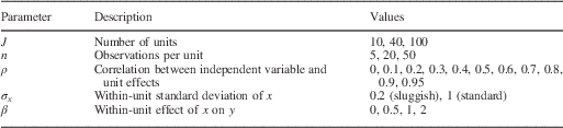
We choose hypothetical values of J, n,
ρ,
 $$\sigma _{x} $$
and β to mimic typical features of
quantitative social science datasets (Table
1). In the terminology of longitudinal data analysis, our simulations
assess both short panels, in which
J>n, as well as long
panels, in which n>J.Footnote
5
To control the variation in x, we set
σ
x
=0.2 to represent a sluggish independent variable, and σ
x
=1 for what we refer to as the standard case in which
individuals differ more greatly within units, making the units more similar on
average. Finally, we allow the correlation between the unit effects
α
j
and the means
 $$\bar{x}_{j} $$
to vary from ρ=0 to
ρ=0.95.Footnote
6
Parameters Manipulated in the Monte Carlo Experiments and their Assumed Values

For each simulated dataset, we estimate the fixed-effects model (Equation 3), the random-effects model
(Equation 4) and the pooled
model (Equation 2), and record
the estimates of
 $$\hat{\beta }$$
produced by each.Footnote
7
We then repeat this process for 2,000 simulated datasets for each
combination of values in Table 1.
Comparing RMSE
We compute the root mean square error (RMSE) of
 $$\hat{\beta }$$
from the fixed-effects, random-effects and pooled models.
When there is a standard amount of variation in the independent variable, there
is no appreciable difference in the quality of inferences between the fixed-
and random-effects models, except at very small numbers of observations per
unit, and extremely high correlation between the independent variable and unit
effects (Figure 1). The conventional
understanding that any correlation between regressors and unit effects
necessarily results in unallowable levels of error in the random-effects
estimator is therefore unfounded. Researchers should feel secure using either
fixed- or random-effects models under standard conditions, as dictated by the
practical and theoretical aspects of a given application. Either way, both
approaches are strictly preferable to the pooled model.
Root mean squared error of slope parameter estimates—standard
case
Note: lines represent the average RMSE of estimates
 $$\hat{\beta }$$
across multiple simulated datasets: fixed effects
(solid line), random effects (dashed) and pooled (dotted). The
horizontal axis is the true amount of correlation between
 $$\bar{x}_{j} $$
and unit effects α
j
. An RMSE of zero indicates that estimates are both unbiased and
subject to negligible estimation uncertainty. Each panel shows a
particular combination of the number of units and number of
observations per unit.

In the case of a sluggish independent variable, there is a range of scenarios
in which the RMSE of
 $$\hat{\beta }$$
is lower with random effects than with fixed effects, even
when the random-effects estimate is biased (Figure 2). The smaller the dataset, the greater the potential
support for a random-effects specification if the correlation between
x and the unit effects is sufficiently low. When the number
of units and/or observations per unit is small—fewer than 200 total
observations, as a rule of thumb—the RMSE of the fixed-effects estimator can be
quite high. This is due to the high variance of the fixed-effects estimator in
small samples, despite its unbiasedness. The random-effects model, in contrast,
can have much lower variance in small datasets. As long as the correlation
between the covariate and unit effects is not too high, the bias in the
random-effects estimator will be small enough that the lower variance of the
estimator will produce a RMSE below that of the fixed-effects model. In the
very smallest datasets, the random-effects estimator outperforms the
fixed-effects estimator even when there are extreme violations of the
assumption of zero correlation.
Root mean squared error of slope parameter estimates—sluggish
case Note: lines represent the average RMSE of estimates
 $$\hat{\beta }$$
across multiple simulated datasets: fixed effects
(solid line), random effects (dashed) and pooled (dotted). The
horizontal axis is the true amount of correlation between
 $$\bar{x}_{j} $$
and unit effects αj. An RMSE of
zero indicates that estimates are both unbiased and subject to
negligible estimation uncertainty. Each panel shows a particular
combination of the number of units and number of observations per
unit.

As the size of the dataset increases, and the variance of the fixed-effects estimates falls, there is less support for the random-effects model. In larger datasets, correlation of greater than 0.2 to 0.3 between the independent variable and unit effects leads to a preference for the fixed-effects model. Increasing the sample size decreases the RMSE of the random-effects estimator, but its bias at high levels of correlation is no longer sufficiently offset by efficiency gains relative to the fixed-effects model. At low (but still non-zero) levels of correlation, however, the random-effects model remains a superior choice.Footnote 8 The conventional wisdom that any violation of the random-effects model’s assumption of zero correlation rules out its use is once again shown to be misguided. The presence of non-zero correlation between the independent variable and unit effects is neither a sufficient nor a necessary condition for choosing a fixed-effects model. Instead, the decision must be based on the amount of data in a study and the level of correlation between regressors and unit effects.
Finally, we note that for a sluggish independent variable, under all conditions, the pooled estimator yields a higher RMSE than the random-effects estimator, though it can outperform the fixed-effects estimator when the data are sufficiently sparse. The superiority of the random-effects model over the pooled model increases with the number of observations per unit.
Conclusion
Scholars generally approach grouped data using either fixed-effects or random-effects models. Advice on which to choose typically emphasizes avoiding bias in estimates of the parameters of interest. Examining the RMSE of both estimators, however, we demonstrate that there is a range of conditions under which it may be worth accepting the bias in the random-effects model if it is associated with a sufficient gain in efficiency, leading to estimates that are closer, on average, to the true value in any particular sample. The most common objection to the use of random effects—the violation of a “critical” modeling assumption: that the regressor and the unit effects are uncorrelated—turns out to be an insufficient justification to prefer fixed over random effects. This condition will hold only under exceptional circumstances, and our simulations demonstrate that even in the presence of rather extreme violations of that assumption, the random-effects estimator can still be preferable to (or at least no worse than) the fixed-effects estimator.
We offer a series of rules of thumb upon which researchers may rely when choosing between a fixed- or random-effects approach. When variation in the independent variable is primarily within units—that is, the units are relatively similar to one another on average—the choice of random versus fixed effects only matters at extremely high levels of correlation between the independent variable and the unit effects. Under these conditions, the appropriate model should be guided by the researcher’s goals. When the independent variable exhibits only minimal within-unit variation, or is sluggish, there is a more nuanced set of considerations. In any particular dataset, the random-effects model will tend to produce superior estimates of β when there are few units or observations per unit, and when the correlation between the independent variable and unit effects is relatively low. Otherwise, the fixed-effects model may be preferable, as the random-effects model does not induce sufficiently high variance reduction to offset its increase in bias.
There are important limitations to the guidance offered here. We have not considered the problem of when the researcher hypothesizes that the effect of x on y varies across units, in which case one would need to employ interactive terms (fixed-effects approach) or a random coefficients model (random-effects approach). In addition, we have only considered the linear-regression model; we have not contemplated generalized linear models for dependent variables that may be dichotomous, ordinal or categorical. Finally, we have only compared two possible specifications—albeit the most commonly used ones in applied social science research. Other modeling choices abound. Nevertheless, the approach we have outlined to evaluate the performance of random- and fixed-effects models under possible violations of the model assumptions can be easily extended to test alternative models on a case-by-case basis.