1. Introduction
Convection is ubiquitous in nature as many flows in geo- or astrophysics are driven by buoyancy. Prominent examples are convection in the Earth’s mantle, the Earth’s core, the interior of giant planets or the outer layer of the Sun. Convection also plays a major role in many technical and engineering applications, and has therefore been the subject of a large number of studies (Ahlers, Grossmann & Lohse Reference Ahlers, Grossmann and Lohse2009; Chillà & Schumacher Reference Chillà and Schumacher2012). The simplest model system for the investigation of buoyancy-driven flows is the Rayleigh–Bénard configuration, a thermally driven flow within a plane fluid layer heated from below and cooled from above.
A recurring theme in both theoretical descriptions and phenomenological pictures of Rayleigh–Bénard convection is the partition of the fluid layer into distinct regions, such as boundary layers close to the wall and a turbulent bulk region in the centre (Grossmann & Lohse Reference Grossmann and Lohse2000; Ahlers et al. Reference Ahlers, Grossmann and Lohse2009), sometimes with a further mixing zone embedded in between the two (Castaing et al. Reference Castaing, Gunaratne, Heslot, Kadanoff, Libchaber, Thomae, Wu, Zaleski and Zanetti1989). These layers are typically defined in terms of experimentally measurable quantities, such as vertical profiles of temperature and velocity, which often show markedly different behaviour in the different regions (Tilgner, Belmonte & Libchaber Reference Tilgner, Belmonte and Libchaber1993; du Puits, Resagk & Thess Reference du Puits, Resagk and Thess2007; Zhou et al. Reference Zhou, Sugiyama, Stevens, Grossmann, Lohse and Xia2011). From a theoretical point of view, however, it is the relative strength of dissipation within the layers that is thought to chiefly control the dynamics of convection, and in particular the macroscopic heat transport (Grossmann & Lohse Reference Grossmann and Lohse2000). Unfortunately, direct experimental measurements of dissipation are still beyond current experimental techniques (Wallace Reference Wallace2009). The connection between the experimentally determined layers and the dissipation processes is thus not straightforward, and requires additional phenomenological modelling, such as the popular assumption that the viscous dissipation is mainly generated by shear within a Prandtl–Blasius-type layer (Grossmann & Lohse Reference Grossmann and Lohse2000; Ahlers et al. Reference Ahlers, Grossmann and Lohse2009; Chillà & Schumacher Reference Chillà and Schumacher2012). Surprisingly little work has been performed on testing the validity of these phenomenological models and their underlying assumptions. The situation is further complicated by the fact that different definitions of the spatial extent of the layers are used in the literature (Kerr & Herring Reference Kerr and Herring2000; Lam et al. Reference Lam, Shang, Zhou and Xia2002; Breuer et al. Reference Breuer, Wessling, Schmalzl and Hansen2004; Zhou & Xia Reference Zhou and Xia2010; Li et al. Reference Li, Shi, du Puits, Resagk, Schumacher and Thess2012; Scheel, Kim & White Reference Scheel, Kim and White2012; Shi, Emran & Schumacher Reference Shi, Emran and Schumacher2012; Wagner, Shishkina & Wagner Reference Wagner, Shishkina and Wagner2012), resulting in different quantitative layer thicknesses strongly depending on the exact definition used.
A first step towards a better understanding of the spatial distribution of viscous dissipation in Rayleigh–Bénard convection has recently been made by Petschel et al. (Reference Petschel, Stellmach, Wilczek, Lülff and Hansen2013), using highly resolved numerical simulations which provide local dissipation rates. The authors show that the thicknesses of layers based directly on dissipation disagree with the thicknesses of more classical boundary layers, and that dissipation-based layer definitions are indeed more suitable to explain the heat transfer observed in their simulations. Although the thickness of the dissipation layer depends, in principle, on its exact definition, it can be regarded as a more general concept than the classical boundary layers since it also applies to turbulent flows due to its definition in terms of statistical quantities. It is furthermore independent of the nature of the boundary conditions and has a straightforward physical interpretation: the dissipation layer simply separates the flow into regions of high (above average) and low (below average) kinetic energy and thermal variance dissipation. Building on these results, Scheel & Schumacher (Reference Scheel and Schumacher2014) have shown recently that classical boundary layers and dissipation layers exhibit opposite Rayleigh number trends for
 $\mathit{Ra}\geqslant 10^{7}$
. The authors hypothesise whether this change in the trend with
 $\mathit{Ra}$
can be related to the transition from soft to hard convective turbulence. Interestingly, this transition cannot be observed for classical velocity boundary layers (Scheel et al.
Reference Scheel, Kim and White2012).
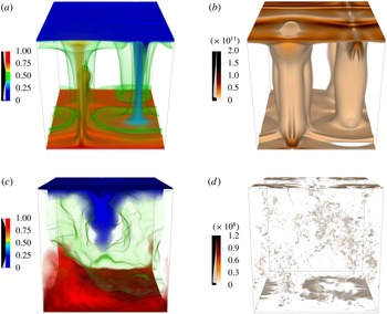
Volume rendering of the temperature fields (a,c) and the kinetic energy dissipation fields (b,d) for high and low Prandtl numbers: (a,b)
 $\mathit{Pr}=150$
and (c,d)
 $\mathit{Pr}=0.01$
.

A thorough understanding of dissipation in Rayleigh–Bénard convection, however, goes beyond a pure identification of its spatial distribution. The physical processes responsible for the spatially inhomogeneous dissipation need to be understood in detail. While global energy conservation requires average dissipative losses to be compensated by corresponding energy sources, both processes often occur in a spatially separated manner. For example, kinetic energy is always produced by buoyancy forces in the bulk, whereas the dissipation is often dominated by deformation work close to the boundaries. A full picture thus needs to include the transport from the source to the dissipation regions, which can be realised by many different physical processes. Again, a very limited number of studies have targeted these questions, with notable examples by Deardorff & Willis (Reference Deardorff and Willis1967) and Kerr (Reference Kerr2001).
In this paper, we extend the existing results by providing a detailed picture of the kinetic energy generation, transport and dissipation in Rayleigh–Bénard convection. The goal of this study is to investigate the transition from bulk-dominated kinetic energy dissipation to boundary-layer-dominated dissipation, which is predicted to be largely controlled by the Prandtl number
 $\mathit{Pr}$
(Grossmann & Lohse Reference Grossmann and Lohse2000). To be conclusive, our study should therefore cover at least the Prandtl number range
 $0.01\geqslant \mathit{Pr}\geqslant 100$
. The need to fully resolve the flow down to the dissipation scale then limits our study to a Rayleigh number
 $\mathit{Ra}=5\times 10^{6}$
. Even for this moderate value of
 $Ra$
, large Reynolds numbers and highly turbulent flows are encountered in the low-Prandtl-number regime (see figure 1). We show that various classical boundary layer definitions can be interpreted directly in terms of kinetic energy fluxes. The kinetic energy transport from the bulk to the dissipation-dominated near-wall region is analysed in detail, and is shown to be accomplished by processes that strongly depend on the Prandtl number.
The paper is organised as follows. In § 3, we discuss our approach in detail. In particular, we show that the pressure term in the kinetic energy transport equation, which hampered the analysis in previous works (Kerr Reference Kerr2001), can be decomposed into several parts, each of which is readily interpreted in terms of elementary physical processes. The spatial distribution of kinetic energy sources, sinks and fluxes is then computed from direct numerical simulations, and the results are presented in §§ 4–6. This detailed analysis reveals which physical processes dominate at a given depth and provides a consistent picture of the generation of kinetic energy, its journey towards the boundaries and its final dissipation. The dynamics is found to be surprisingly rich, requiring a decomposition of the domain into a considerable number of sublayers, each characterised by different physical processes at work. Detailed conclusions are presented in § 7.
2. Method
2.1. Governing equations
The Rayleigh–Bénard problem is governed by the non-dimensional Oberbeck–Boussinesq equations
 $$\begin{eqnarray}\displaystyle & \displaystyle \frac{\partial u_{i}}{\partial t}+u_{j}\frac{\partial u_{i}}{\partial x_{j}}=\frac{\partial {\it\tau}_{ij}}{\partial x_{j}}+\mathit{Pr}\mathit{Ra}\,{\it\theta}{\it\delta}_{i3}, & \displaystyle\end{eqnarray}$$
 $$\begin{eqnarray}\displaystyle & \displaystyle \frac{\partial {\it\theta}}{\partial t}+u_{j}\frac{\partial {\it\theta}}{\partial x_{j}}=\frac{\partial ^{2}{\it\theta}}{\partial x_{j}^{2}}+u_{3}, & \displaystyle\end{eqnarray}$$
 $$\begin{eqnarray}\displaystyle & \displaystyle \frac{\partial u_{i}}{\partial x_{i}}=0, & \displaystyle\end{eqnarray}$$
 $u_{i}$
is the velocity component,
 ${\it\theta}=T-1+x_{3}$
is the deviation of the actual temperature
 $T$
from the conductive temperature profile and
 ${\it\tau}_{ij}=-P{\it\delta}_{ij}+2\,\mathit{Pr}\,\unicode[STIX]{x1D626}_{ij}$
is the stress tensor for incompressible Newtonian fluids. Here,
 $\unicode[STIX]{x1D626}_{ij}=((\partial u_{i}/\partial x_{j})+(\partial u_{j}/\partial x_{i}))/2$
is the rate-of-strain tensor and
 $P$
is the pressure.
The equations have been made dimensionless by using the system height
 $L$
as a length scale and the thermal diffusion time
 $L^{2}/{\it\kappa}$
as a time scale, where
 ${\it\kappa}$
denotes the thermal diffusivity. The system is then characterised by two non-dimensional control parameters only, the Rayleigh number and the Prandtl number,
 $$\begin{eqnarray}\mathit{Ra}=\frac{{\it\alpha}g{\rm\Delta}TL^{3}}{{\it\nu}{\it\kappa}},\quad \mathit{Pr}=\frac{{\it\nu}}{{\it\kappa}}.\end{eqnarray}$$
Here,
 ${\it\alpha}$
denotes the thermal expansion coefficient,
 $g$
the acceleration of gravity,
 ${\rm\Delta}T$
the temperature difference between the bottom and the top and
 ${\it\nu}$
the kinematic viscosity. The top and bottom boundaries are impermeable and are kept at a fixed temperature. No-slip boundary conditions are used for the velocity field.
2.2. Numerical model
To investigate the properties of the kinetic energy transport in detail, the time evolution of the velocity, pressure and temperature fields is studied by means of three-dimensional direct numerical simulations. For a fixed Rayleigh number
 $\mathit{Ra}=5\times 10^{6}$
, the Prandtl number range
 $0.01\leqslant \mathit{Pr}\leqslant 150$
is systematically explored. The simulations in a cubic Cartesian box with periodic boundary conditions in the horizontal directions are carried out using an accurate pseudo-spectral method. Fourier series are used for spatial discretisation in the horizontal direction, whereas Chebyshev basis functions are used in the vertical direction. Temporal discretisation is accomplished through a second-order semi-implicit Adams–Bashforth time stepping with backward differentiation. For further details on the numerical method, see Stellmach & Hansen (Reference Stellmach and Hansen2008). Since Chebyshev basis functions naturally provide high resolution near the boundaries, the bottleneck in resolving the local kinetic energy balance is a sufficiently high resolved bulk region. Even for this moderate Rayleigh number, spatial resolutions of up to
 $576^{3}$
grid points were necessary to adequately resolve the Kolmogorov scales within the bulk at low
 $\mathit{Pr}$
(Grötzbach Reference Grötzbach1983; Shishkina, Stevens & Grossmann Reference Shishkina, Stevens, Grossmann and Lohse2010).
3. Kinetic energy balance and decomposition of the flux
In this section we introduce the well-known kinetic energy equation for Rayleigh–Bénard convection and review the different contributions to the kinetic energy balance. We will first consider the effects of kinetic energy production, dissipation and fluxes. To obtain further insight we then decompose the fluxes into several contributions, each of which is caused by a different physical effect.
3.1. Kinetic energy balance
By multiplying the Navier–Stokes equation (2.1) by the velocity
 $u_{i}$
and using the incompressibility (2.3), we obtain the kinetic energy equation
 $$\begin{eqnarray}\frac{\partial }{\partial t}\mathit{E}_{kin}+\frac{\partial }{\partial x_{i}}(u_{i}\mathit{E}_{kin}-u_{j}{\it\tau}_{ij})=-2\mathit{Pr}\,\unicode[STIX]{x1D626}_{ij}^{2}+\mathit{Pr}\mathit{Ra}\,{\it\theta}u_{3},\end{eqnarray}$$
where
 $\mathit{E}_{kin}=u_{i}^{2}/2$
denotes the kinetic energy. This equation represents a budget equation of the form (Deardorff & Willis Reference Deardorff and Willis1967; Kerr Reference Kerr2001)
 $$\begin{eqnarray}\frac{\partial }{\partial t}\mathit{E}_{kin}+\frac{\partial }{\partial x_{i}}J_{i}=-{\it\epsilon}+S,\end{eqnarray}$$
where the right-hand side comprises a sink
 ${\it\epsilon}$
and a source
 $S$
. The left-hand side includes a temporal change of the kinetic energy as well as a flux term, which spatially redistributes kinetic energy. By comparing (3.1) with (3.2) we have
 $$\begin{eqnarray}S=\mathit{Pr}\mathit{Ra}\,{\it\theta}u_{3},\end{eqnarray}$$
which means that the kinetic energy source, which comes from the work done by buoyancy forces, is proportional to the advective heat transport. The sink is identified as
 $$\begin{eqnarray}{\it\epsilon}=2\mathit{Pr}\,\unicode[STIX]{x1D626}_{ij}^{2}.\end{eqnarray}$$
All processes that do not change the net budget, but spatially redistribute kinetic energy, can be expressed as the divergence of the total kinetic energy flux
 $$\begin{eqnarray}J_{i}=u_{i}\mathit{E}_{kin}-u_{j}{\it\tau}_{ij}.\end{eqnarray}$$
This means that advection and stress transport kinetic energy from regions where net energy is produced to regions where net energy is dissipated.
3.2. Flux decomposition
The flux can be further decomposed, and we start by considering the pressure contributions. A major difficulty in understanding the kinetic energy flux (3.5) is the non-locality of the pressure, which is governed by the elliptic equation
 $$\begin{eqnarray}\frac{\partial ^{2}P}{\partial x_{i}^{2}}=-\frac{\partial u_{j}}{\partial x_{i}}\frac{\partial u_{i}}{\partial x_{j}}+\mathit{Pr}\mathit{Ra}\,\frac{\partial {\it\theta}}{\partial x_{3}}\end{eqnarray}$$
that follows from taking the divergence of the momentum equation (2.1). We can split up the pressure into three contributions, one due to buoyancy,
 $$\begin{eqnarray}\frac{\partial ^{2}P}{\partial x_{i}^{2}}^{(buo)}=\mathit{Pr}\mathit{Ra}\,\frac{\partial {\it\theta}}{\partial x_{3}}\quad \text{with }\left.\frac{\partial P}{\partial x_{3}}^{(buo)}\right|_{x_{3}=0,1}=0,\end{eqnarray}$$
and another one due to advection,
 $$\begin{eqnarray}\frac{\partial ^{2}P}{\partial x_{i}^{2}}^{(adv)}=-\frac{\partial u_{j}}{\partial x_{i}}\frac{\partial u_{i}}{\partial x_{j}}\quad \text{with }\left.\frac{\partial P}{\partial x_{3}}^{(adv)}\right|_{x_{3}=0,1}=0.\end{eqnarray}$$
Finally, the pressure induced by viscous stresses at the boundary is given by
 $$\begin{eqnarray}\frac{\partial ^{2}P}{\partial x_{i}^{2}}^{(vis)}=0\quad \text{with }\left.\frac{\partial P}{\partial x_{3}}^{(vis)}\right|_{x_{3}=0,1}=\mathit{Pr}\,\frac{\partial ^{2}u_{3}}{\partial x_{3}^{2}}.\end{eqnarray}$$
The stress tensor can thus be written as
 $$\begin{eqnarray}{\it\tau}_{ij}=-(P^{(adv)}+P^{(buo)}+P^{(vis)})\,{\it\delta}_{ij}+2\,\mathit{Pr}\,\unicode[STIX]{x1D626}_{ij}.\end{eqnarray}$$
Using this expression, the kinetic energy flux can be expressed as
 $$\begin{eqnarray}J_{i}=u_{i}\mathit{E}_{kin}+u_{j}[(P^{(adv)}+P^{(buo)}+P^{(vis)})\,{\it\delta}_{ij}-2\,\mathit{Pr}\,\unicode[STIX]{x1D626}_{ij}].\end{eqnarray}$$
The overall kinetic energy flux is hence composed of the flux caused by advective processes, the flux due to buoyancy pressure and the flux due to viscous processes. The viscous flux can be further separated into fluxes involving normal and shear stresses. Here, viscous normal stresses are connected to the diagonal of the rate-of-strain tensor,
 $\text{diag}(\unicode[STIX]{x1D626}_{11},\unicode[STIX]{x1D626}_{22},\unicode[STIX]{x1D626}_{33})_{ij}$
, while viscous shear stresses are connected to the off-diagonal elements of the rate-of-strain tensor
 $\unicode[STIX]{x1D626}_{ij}-\text{diag}(\unicode[STIX]{x1D626}_{11},\unicode[STIX]{x1D626}_{22},\unicode[STIX]{x1D626}_{33})_{ij}$
. The individual flux contributions are then defined as
 $$\begin{eqnarray}\displaystyle & \displaystyle J_{i}^{(adv)}=u_{i}\mathit{E}_{kin}+u_{i}\,P^{(adv)}, & \displaystyle\end{eqnarray}$$
 $$\begin{eqnarray}\displaystyle & \displaystyle J_{i}^{(buo)}=u_{i}\,P^{(buo)}, & \displaystyle\end{eqnarray}$$
 $$\begin{eqnarray}\displaystyle & \displaystyle J_{i}^{(norm)}=-2\,\mathit{Pr}\,u_{j}\,\text{diag}(\unicode[STIX]{x1D626}_{11},\unicode[STIX]{x1D626}_{22},\unicode[STIX]{x1D626}_{33})_{ij}+u_{i}\,P^{(vis)}, & \displaystyle\end{eqnarray}$$
 $$\begin{eqnarray}\displaystyle & \displaystyle J_{i}^{(shear)}=-2\,\mathit{Pr}\,u_{j}(\unicode[STIX]{x1D626}_{ij}-\text{diag}(\unicode[STIX]{x1D626}_{11},\unicode[STIX]{x1D626}_{22},\unicode[STIX]{x1D626}_{33})_{ij}). & \displaystyle\end{eqnarray}$$
 $$\begin{eqnarray}\frac{\partial }{\partial t}\mathit{E}_{kin}+\frac{\partial }{\partial x_{i}}(J_{i}^{(adv)}+J_{i}^{(buo)}+J_{i}^{(norm)}+J_{i}^{(shear)})=-{\it\epsilon}+S,\end{eqnarray}$$
i.e. the kinetic energy budget consists of a production term, a dissipation term and four spatial redistribution terms.
3.3. Horizontally and temporally averaged kinetic energy balance
In the following we will analyse the horizontally and temporally averaged kinetic energy balance. These averages are denoted by the following nomenclature:
 $\langle \dots \rangle _{v}$
represents an average over the entire volume and over time, and
 $\langle \dots \rangle$
represents an average over horizontal planes and time. In the statistically stationary case the kinetic energy budget, for this horizontally homogeneous system, simplifies to
 $$\begin{eqnarray}\frac{\partial }{\partial x_{3}}\langle J_{3}\rangle =-\langle {\it\epsilon}\rangle +\langle S\rangle ,\end{eqnarray}$$
where all quantities depend on height only. The averaged individual fluxes can be simplified to
 $$\begin{eqnarray}\displaystyle & \displaystyle \langle J_{3}^{(adv)}\rangle =\langle u_{3}\mathit{E}_{kin}\rangle +\langle u_{3}\,P^{(adv)}\rangle , & \displaystyle\end{eqnarray}$$
 $$\begin{eqnarray}\displaystyle & \displaystyle \langle J_{3}^{(buo)}\rangle =\langle u_{3}\,P^{(buo)}\rangle , & \displaystyle\end{eqnarray}$$
 $$\begin{eqnarray}\displaystyle & \displaystyle \langle J_{3}^{(norm)}\rangle =-\mathit{Pr}\,\frac{\partial }{\partial x_{3}}\langle u_{3}^{2}\rangle +\langle u_{3}\,P^{(vis)}\rangle , & \displaystyle\end{eqnarray}$$
 $$\begin{eqnarray}\displaystyle & \displaystyle \langle J_{3}^{(shear)}\rangle =-\mathit{Pr}\,\frac{\partial }{\partial x_{3}}\langle \mathit{E}_{kin}\rangle . & \displaystyle\end{eqnarray}$$
To ensure comparability between different Prandtl numbers, all profiles are normalised by the volume-averaged viscous dissipation rate, which is linked to the Nusselt number
 $\mathit{Nu}$
by the relation
 $$\begin{eqnarray}\langle {\it\epsilon}\rangle _{v}=\mathit{Pr}\,\mathit{Ra}(\mathit{Nu}-1),\end{eqnarray}$$
where the Nusselt number is defined as the sum of advective and conductive heat transport,
 $$\begin{eqnarray}\mathit{Nu}-1=\langle {\it\theta}u_{3}\rangle -\frac{\partial }{\partial x_{3}}\langle {\it\theta}\rangle .\end{eqnarray}$$
Since the total heat flux through any plane must be constant at every height, the Nusselt number (defined in terms of horizontally and temporally averaged quantities) equals its volume average at every height.
4. Kinetic energy balance profiles
In this section we use direct numerical simulations to explicitly compute the individual contributions to the kinetic energy balance (3.17)–(3.21). We first focus our discussion on the source, the sink and the total flux. After that we turn to a detailed discussion of the individual flux contributions (3.18)–(3.21).
4.1. Source
The production profile,
 $\mathit{Ra}\mathit{Pr}\langle {\it\theta}u_{3}\rangle$
, is displayed in figure 2 for different Prandtl numbers. It is proportional to the advective heat transport,
 $\langle {\it\theta}u_{3}\rangle$
. Since the averaged total heat flux through any plane must be constant at every height, the kinetic energy production is also directly connected to the conductive heat transport:
 $$\begin{eqnarray}\frac{\langle S\rangle }{\mathit{Pr}\,\mathit{Ra}}=(\mathit{Nu}-1)+\frac{\partial }{\partial x_{3}}\langle {\it\theta}\rangle .\end{eqnarray}$$
The kinetic energy source profile can thus be calculated from the temperature profile and the Nusselt number.
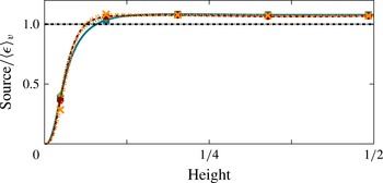
Profiles of the kinetic energy source for different Prandtl numbers (blue square,
 $Pr=0.1$
; green diamond,
 $Pr=1$
; red circle,
 $Pr=10$
; orange cross,
 $Pr=100$
). The symbols on the lines help to identify the profiles for different Prandtl numbers more easily and do not represent the grid resolution, which is much finer.

Figure 2 shows the kinetic energy source profile for different Prandtl numbers. The profiles are almost independent of the Prandtl number. All cases exhibit two distinct regions: one associated with an isothermal well-mixed bulk in the centre of the domain and a second one related to a near-wall layer, which is characterised by strong temperature gradients. The bulk region exhibits an almost constant kinetic energy production, while the kinetic energy production in the near-wall layer rapidly decays towards the wall. Nearly the entire temperature drop occurs within this near-wall region. Because of the impermeable walls (
 $u_{3}|_{x_{3}=0,1}=0$
), the kinetic energy source must be zero at the boundaries. Both regions can be naturally separated by the crossing of the source profiles with the volume-averaged dissipation (3.22) (which equals the volume-averaged source). By relation (4.1), this is also the vertical position of the maximum of
 $|\langle {\it\theta}\rangle |$
, which is sometimes used to define the thermal boundary layer. Since
 $\partial /\partial _{x_{3}}\langle {\it\theta}\rangle \leqslant 1$
in the centre of the domain for a completely mixed fluid, relation (4.1) also reveals the Nusselt number as an upper bound for the source profile in the bulk.
4.2. Sink
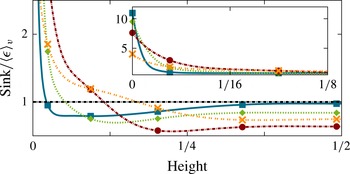
The sink in the kinetic energy budget is given by the viscous dissipation term. Its profile is shown in figure 3 for different Prandtl numbers. Similarly to the kinetic energy source, the sink profile can be separated into two regions: a bulk region, characterised by low dissipation rates, and the dissipation layer introduced by Petschel et al. (Reference Petschel, Stellmach, Wilczek, Lülff and Hansen2013) with significantly enhanced dissipation close to the boundary. The edge of the dissipation layer is defined as the vertical position at which the dissipation rate equals its volume-averaged value.
Profiles of the kinetic energy sink, i.e. the viscous dissipation rate, for different Prandtl numbers (blue square,
 $Pr=0.1$
; green diamond,
 $Pr=1$
; red circle,
 $Pr=10$
; orange cross,
 $Pr=100$
). The inset of the graph shows a boundary layer blowup to display the respective ‘wall dissipation’.

In contrast to the kinetic energy production, the transition region in figure 3 distinctively varies with the Prandtl number. For high Prandtl numbers the viscous dissipation increases monotonically towards the boundaries and smears out the transition of the bulk and the dissipation layer. The opposite is observed for low Prandtl numbers where the transition is much sharper.
In the centre of the domain the viscous dissipation rate profile is constant for all Prandtl numbers. However, the amplitude strongly depends on
 $\mathit{Pr}$
. For
 $\mathit{Pr}=0.1$
the bulk dissipation rate almost equals its volume average, whereas for Prandtl numbers of
 $\mathit{Pr}=1$
and
 $\mathit{Pr}=10$
the bulk dissipation rate is much smaller. For even larger Prandtl numbers (
 $\mathit{Pr}\geqslant 20$
, exact transition point not indicated in figure 3) this tendency reverses, and the viscous dissipation rate in the centre of the domain begins to increase again, as illustrated by the case
 $\mathit{Pr}=100$
in figure 3.
In the near-wall region the kinetic dissipation profile increases significantly towards the boundaries for all Prandtl numbers, as can be seen in the inset of figure 3. The dissipation immediately at the wall,
 ${\it\epsilon}|_{x_{3}=0,1}$
, decreases for increasing Prandtl numbers. Since the kinetic energy production vanishes at the boundary, the wall dissipation must be balanced entirely by the kinetic energy fluxes.
4.3. Flux
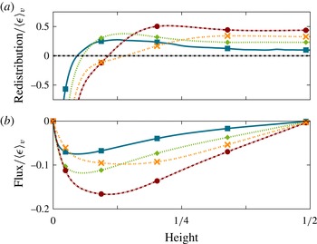
In addition to the production rate and the viscous dissipation rate, the redistribution of kinetic energy, i.e. the divergence of kinetic energy flux, completes the kinetic energy budget. The profile of the total flux divergence (3.17) and the total flux profile are shown in figure 4 for different Prandtl numbers. A negative flux indicates a transport of kinetic energy towards the boundaries whereas a positive flux indicates a transport towards the centre. As can be inferred from the figure, the system transports kinetic energy from the centre towards the walls in the entire domain. Since the Rayleigh–Bénard configuration is a closed system with up–down symmetry, all kinetic energy flux profiles have to vanish at the boundaries and at the centre of the domain.
Profiles of the kinetic energy redistribution, i.e. the divergence of flux, (a) and the vertical kinetic energy flux (b) for different Prandtl numbers (blue square,
 $Pr=0.1$
; green diamond,
 $Pr=1$
; red circle,
 $Pr=10$
; orange cross,
 $Pr=100$
).

A negative divergence of the flux characterises deposition of kinetic energy whereas a positive flux divergence signifies a removal of surplus kinetic energy. Because the horizontally and temporally averaged flux divergence in the statistical stationary case is equal to the difference of the kinetic energy source and viscous dissipation rates (cf. (3.2)), it exhibits negative values near the boundaries and positive values in the bulk, as can be seen in figure 4(a). These regions are separated by the zero crossing of the divergence of the flux, corresponding to the maximum of the absolute kinetic energy flux. The distance between the boundary of the domain and the vertical position of this maximum increases for increasing Prandtl number.
Since the kinetic energy source does not strongly depend on the Prandtl number, the Prandtl dependence of the viscous dissipation must be linked to that of the flux. Accordingly, several characteristics of the kinetic energy sink profile in figure 3 can also be observed in the flux profile. Similarly to the sink profile, the flux profile also strongly depends on
 $\mathit{Pr}$
: for high Prandtl number the flux profiles are much flatter than for low Prandtl number and do not exhibit a distinct maximum. With decreasing
 $\mathit{Pr}$
this maximum becomes more pronounced, which indicates that for decreasing Prandtl number the boundary between the bulk and the near-wall region becomes sharper. Again, the Prandtl number tendency of the flux reverses for very high
 $\mathit{Pr}$
. The maximum of the flux increases with increasing Prandtl numbers
 ${\leqslant}10$
and decreases again for very high Prandtl numbers. This indicates a regime transition between
 $\mathit{Pr}=10$
and
 $\mathit{Pr}=100$
.
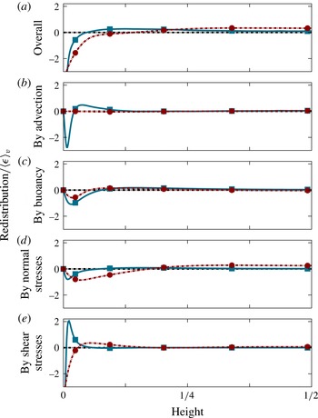
To characterise the Prandtl number dependence of the kinetic energy balance away from the boundaries, it is instructive to investigate the profiles of the individual transport mechanisms. The kinetic energy flux consists of four partial fluxes, as shown in § 3.2. The profiles of the individual flux divergences along with their sum are shown in figure 5 for high and low Prandtl numbers, which will be discussed in the following sections.
4.3.1. Kinetic energy transport by the individual fluxes for low Prandtl numbers
We first focus on our results at
 $\mathit{Pr}=0.1$
. As we have discussed in the previous sections, the kinetic energy is mainly produced in the bulk region and mainly dissipated in the near-wall region. The total flux redistributes the kinetic energy from the bulk into the near-wall region. We will discuss in the following the individual redistributions for
 $\mathit{Pr}=0.1$
starting from the centre of the domain and proceeding towards the boundaries. As we have seen above, in the central region of the domain the redistribution of kinetic energy decreases with decreasing Prandtl number. The small redistribution for low Prandtl numbers shows that there is only a small surplus of kinetic energy in this region. As a consequence, the production is almost balanced by the dissipation. This can be explained by an increasingly statistically homogeneous flow in the bulk region with decreasing
 $\mathit{Pr}$
(cf. figure 1).
Redistribution of kinetic energy given by the profiles of the divergence of fluxes for high (blue solid line) and low (red dashed line) Prandtl numbers (blue square,
 $Pr=0.1$
; red circle,
 $Pr=100$
). Graph (a) shows the redistribution by the sum of all individual fluxes, whereas graphs (b–e) show the redistribution by individual fluxes (cf. § 3.2).

Figure 5 shows that the small remaining surplus of kinetic energy in the centre is transported towards the walls mostly by buoyancy-pressure flux and normal-stress flux. Both fluxes deposit the removed kinetic energy in the near-wall region. The advective flux does not influence the centre, but rather strongly redistributes kinetic energy closer to the walls. It dominates the transport in the near-wall region between the turbulent bulk and the thin boundary layer close to the rigid wall.
As discussed earlier, the flux divergence must balance the dissipation at the boundaries. An analytical evaluation of the individual flux contributions, exploiting the no-slip boundary conditions, yields further insights. In fact, it can be shown that all flux divergences vanish at the boundary, except for the divergence of viscous shear flux. We can conclude that the ‘wall dissipation’ is balanced by the divergence of the shear-stress flux only:
 $$\begin{eqnarray}\langle {\it\epsilon}\rangle |_{x_{3}=0,1}=\left.\frac{\partial }{\partial x_{3}}\langle J_{3}^{(shear)}\rangle \right|_{x_{3}=0,1}=\left.-\mathit{Pr}\left\langle \left(\frac{\partial }{\partial x_{3}}\left(u_{2}+u_{1}\right)\right)^{2}\right\rangle \right|_{x_{3}=0,1}.\end{eqnarray}$$
Thus, the redistribution by shear stress deposits kinetic energy much closer to the wall than all other fluxes and is particularly important in the very-near-wall region. It may thus be regarded as a boundary-driven process.
On the basis of the individual flux profiles in figure 5, it can be concluded that the vertical structure of the redistributions can be separated into three regions. In the central region only little kinetic energy is transported towards the walls, reflecting a tendency towards homogeneous flow at low
 $\mathit{Pr}$
. Closer to the wall, kinetic energy is transported by the advective flux from the bulk towards the boundary. In the direct vicinity of the wall, the shear-stress flux redistributes kinetic energy to the boundary, where the strongest dissipation takes place.
Interestingly, our results show that the influence of the boundaries extends beyond the small viscous shear region that is central to many theories of convective heat transport. Beyond this region, the walls induce flow inhomogeneities that cause a strong advective kinetic energy flux. It is crucial to account for this effect for any comprehensive view of kinetic energy transport in low-Prandtl-number convection.
4.3.2. Kinetic energy transport by the individual fluxes for high Prandtl numbers
Similarly to the low-
 $\mathit{Pr}$
case, the individual redistributions for high Prandtl numbers will be discussed from the centre to the boundary. For
 $\mathit{Pr}=100$
the production in the bulk region is significantly higher than the dissipation. This leads to enhanced vertical redistribution of kinetic energy within the bulk. Figure 5 shows that the kinetic energy is transported almost exclusively by normal-stress flux from the centre towards the boundary. All other fluxes approximately vanish in the bulk. The vertical position of the minimum of the divergence of the normal-stress flux, i.e. the position of maximal deposition of kinetic energy, is close to the boundary. Thus, normal-stress flux transports kinetic energy from the centre through the entire domain into the very-near-wall region.
Closer to the wall, buoyancy pressure also starts to redistribute kinetic energy, but in a limited region. Redistribution by advection is negligible in the entire domain. Similarly to the low-
 $\mathit{Pr}$
number case, shear-stress flux redistributes kinetic energy from the very-near-wall region towards the boundary. Although the shear-stress redistribution profile maintains its general shape across Prandtl numbers, the region that is dominated by shear-stress flux expands with increasing Prandtl number.
The profiles of the individual redistributions suggest that the kinetic energy transport is dominated by viscous effects for high Prandtl numbers. In contrast to the crucial role of advective flux in the low-
 $\mathit{Pr}$
case, the normal-stress flux transports kinetic energy from the centre directly to the very-near-wall region. The transport of kinetic energy from the centre all the way into the boundary region may be seen as an indicator for flow features extending throughout the whole domain, as observed for high Prandtl numbers in previous studies (Kerr & Herring Reference Kerr and Herring2000; Breuer et al.
Reference Breuer, Wessling, Schmalzl and Hansen2004).
5. Dissipation, source and flux layers
As we have seen in the previous section, the profiles vary considerably as a function of height. This allows us to separate the domain into distinct regions. We now introduce the concept of layers for the individual contributions as a quantitative measure to distinguish these regions, generalising the dissipation layers introduced by Petschel et al. (Reference Petschel, Stellmach, Wilczek, Lülff and Hansen2013). We will then analyse the Prandtl number dependence of the layers related to the source, sink and flux. After that we will turn to a detailed discussion of the layers associated with the individual flux contributions (3.18)–(3.21). We close the section by a comparison with classical velocity boundary layers.
5.1. Definition of the layers
The observations on the profiles of the kinetic energy budget in the previous section (§ 4) can be used to separate the domain into two regions, namely a layer in which the profile is above the volume average and a layer in which the profile is below the volume average. Petschel et al. (Reference Petschel, Stellmach, Wilczek, Lülff and Hansen2013) have used the crossing between these two regions to define the so-called dissipation layer (
 $\text{DL}$
). More specifically, the edge of the dissipation layer is defined by the vertical position at which the dissipation rate equals its volume-averaged value,
 $$\begin{eqnarray}\langle {\it\epsilon}\rangle (x_{3,DL})\stackrel{!}{=}\langle {\it\epsilon}\rangle _{v}.\end{eqnarray}$$
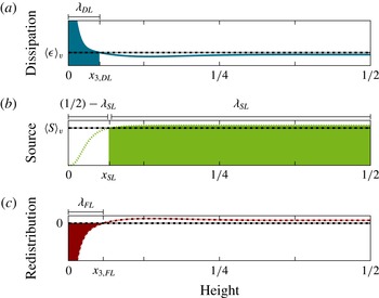
The distance from the closest boundary then defines the viscous dissipation layer thickness
 ${\it\lambda}_{DL}$
, as illustrated in figure 6. The interpretation of the dissipation layer is rather simple: fluid within the dissipation layer is characterised by a dissipation above the volume average.
Profiles of the dissipation, the source and the divergence of the flux for
 $\mathit{Pr}=1$
along with the definition of the layers defined by the respective profiles ((a) blue colour, DL; (b) green colour, SL; (c) red colour, FL).

Similarly to the dissipation layer, we introduce the source layer (
 $\text{SL}$
), which is characterised by enhanced kinetic energy production. The edge of the source layer is defined analogously to the dissipation layer by the vertical position at which the kinetic energy source equals its volume-averaged value,
 $$\begin{eqnarray}\langle S\rangle (x_{3,SL})\stackrel{!}{=}\langle S\rangle _{v}.\end{eqnarray}$$
Kinetic energy production due to buoyancy is an essential feature of the bulk region. Consequently, we define the distance from the centre of the domain as the source layer thickness
 ${\it\lambda}_{SL}$
, cf. figure 6. The dissipation and the source layer separate the flow into regions of high (above average) and low (below average) kinetic energy dissipation and production respectively.
The kinetic energy flux transports kinetic energy from the source layer into the dissipation layer. Thus, we can define a flux layer (
 $\text{FL}$
), which separates the domain into regions of flux-induced reduction and accumulation of kinetic energy. The edge of the flux layer is then defined by the vertical position where the divergence of the flux equals zero, which corresponds to a local extremum of the flux, i.e.
 $$\begin{eqnarray}\frac{\partial }{\partial x_{3}}\langle J_{3}\rangle (x_{3,FL})\stackrel{!}{=}0\quad \text{respectively}~\langle J_{3}\rangle (x_{3,FL})\stackrel{!}{=}\text{max}|\langle J_{3}\rangle |.\end{eqnarray}$$
The distance from the closest boundary then sets the kinetic energy flux layer thickness
 ${\it\lambda}_{FL}$
. From the definitions above, it can be shown that the edge of the flux layer has to be located in between the edges of the dissipation and source layers.
5.2. Prandtl dependence of the dissipation, source and flux layer thicknesses
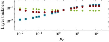
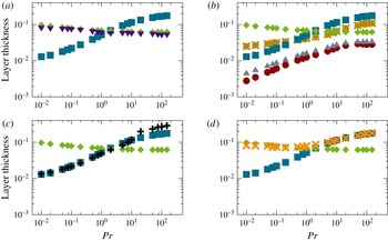
Figure 7 shows the thickness of the dissipation layer
 ${\it\lambda}_{DL}$
and of the flux layer
 ${\it\lambda}_{FL}$
along with the distance between the boundary and the source layer (
 $(1/2)-{\it\lambda}_{SL}$
) as a function of the Prandtl number. The figure reveals that at low
 $\mathit{Pr}$
, the regions of kinetic energy production and dissipation are spatially separated, while for high
 $\mathit{Pr}\geqslant 2$
, they overlap. When they are spatially separated, the region in between is characterised by low production and dissipation of kinetic energy, as can be seen by a closer inspection of the profiles (not shown here). The overlap region, observed for high Prandtl numbers, features high energy production and dissipation levels.
Thicknesses of different layers versus the Prandtl number. Blue squares represent the thickness of the dissipation layer
 ${\it\lambda}_{DL}$
, red circles denote the flux layer thickness
 ${\it\lambda}_{FL}$
and green diamonds indicate the distance between the boundary and the source layer
 $(1/2)-{\it\lambda}_{SL}$
.

The flux layer thickness displays no monotonic
 $\mathit{Pr}$
dependence. For low Prandtl numbers it compares approximately with the magnitude of the gap between the boundary and the source layer (i.e.
 ${\it\lambda}_{FL}\approx (1/2)-{\it\lambda}_{SL}$
). For high Prandtl numbers it has roughly the same thickness as the dissipation layer.
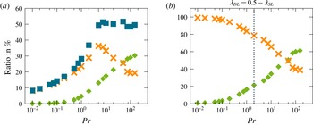
The ratio of dissipation layer contributions normalised by the volume-averaged dissipation rate versus the Prandtl number (a) and the rate of kinetic energy accumulation in the dissipation layer normalised by the dissipation rate averaged over the dissipation layer (b). The blue squares denote the dissipation in the dissipation layer
 $|\langle {\it\epsilon}\rangle _{DL}/\langle {\it\epsilon}\rangle _{v}|$
, while the green diamonds denote the kinetic energy produced within the dissipation layer (
 $|\langle S\rangle _{DL}/\langle {\it\epsilon}\rangle _{v}|$
(a);
 $|\langle S\rangle _{DL}/\langle {\it\epsilon}\rangle _{DL}|$
(b)). Additionally, the orange crosses indicate the accumulation of kinetic energy by the flux in the dissipation layer (
 $|\langle \partial _{3}J_{3}\rangle _{DL}/\langle {\it\epsilon}\rangle _{v}|$
(a);
 $|\langle \partial _{3}J_{3}\rangle _{DL}/\langle {\it\epsilon}\rangle _{DL}|$
(b)). The vertical grey dashed line indicates the Prandtl number where the source and dissipation layers are of the same thickness.

Petschel et al. (Reference Petschel, Stellmach, Wilczek, Lülff and Hansen2013) have argued for a transition from bulk-dominated dissipation at low
 $\mathit{Pr}$
to significant dissipation within the dissipation layer at high
 $\mathit{Pr}$
. As can be seen in figure 8(a), high Prandtl numbers are characterised by a saturation of the relative dissipation within the dissipation layer. Interestingly, the dissipation only saturates because the production increases; due to accumulation of kinetic energy by flux alone such a high dissipation in the dissipation layer is not possible. Hence, the spatial overlap of production and dissipation has a strong influence on the net dissipation in the dissipation layer. To examine the influence of this overlap closer, figure 8(b) shows the accumulation of kinetic energy in the dissipation layer by flux and production, the sum of which is balanced by dissipation. As expected, the production within the dissipation layer vanishes for low Prandtl numbers because the source and the dissipation layer are spatially separated. Consequently, the dissipation in the dissipation layer is balanced only by the accumulation of kinetic energy by flux for low Prandtl numbers. For high Prandtl numbers, however, more kinetic energy is produced in the dissipation layer than is accumulated by flux. This finding suggests that a dominance of the dissipation layer, as described by Petschel et al. (Reference Petschel, Stellmach, Wilczek, Lülff and Hansen2013), goes along with an overlap of the source and the dissipation layer.
5.3. Flux layer thickness for individual fluxes
To understand the influence of the individual fluxes on the kinetic energy profiles more deeply, figure 9 shows the thicknesses of the four individual flux layers (
 ${\it\lambda}_{FL,shear}$
,
 ${\it\lambda}_{FL,adv}$
,
 ${\it\lambda}_{FL,buo}$
and
 ${\it\lambda}_{FL,norm}$
) along with the dissipation layer (
 ${\it\lambda}_{DL}$
) and the distance from the boundary to the source layer (
 $(1/2)-{\it\lambda}_{SL}$
). Similarly to the overall flux, the edge of the flux layers indicates the height of the transition from removal to accumulation by the corresponding flux according to (5.3).
Thicknesses of different layers versus the Prandtl number. The dissipation layer, represented by blue squares
 $({\it\lambda}_{DL})$
, and the source layer, represented by green diamonds
 $((1/2)-{\it\lambda}_{SL})$
, can be seen in all graphs. Additionally, the flux layer thicknesses are denoted by purple triangles for the flux by buoyancy
 $({\it\lambda}_{FL,buo})$
, black crosses for the flux by advection
 $({\it\lambda}_{FL,adv})$
, orange crosses for the flux by normal stresses
 $({\it\lambda}_{FL,norm})$
and red dots for the flux by shear
 $({\it\lambda}_{FL,shear})$
. In (b), grey triangles indicate a classical viscous boundary layer (
 ${\it\lambda}_{BL}^{lin}$
), measured by the slope method, and golden stars indicate the position of the maximum of the horizontal velocity profile (
 ${\it\lambda}_{BL}^{max}$
).

As can be seen in figure 9(a), the thickness of the buoyancy-pressure flux layer varies only little with the Prandtl number, and corresponds in magnitude to the gap between the source layer and the boundary. The good agreement with the source layer suggests that buoyancy pressure is related to the kinetic energy production and therefore to the advective heat transport (cf. § 4.1). The advective flux layer (figure 9
c) coincides with the dissipation layer for low
 $\mathit{Pr}$
, whereas the normal-stress flux layer (figure 9
d) coincides with the dissipation layer for high
 $\mathit{Pr}$
. This suggests that both fluxes – the advective flux for low
 $\mathit{Pr}$
and the normal-stress flux for high
 $\mathit{Pr}$
– transport kinetic energy into the dissipation layer. For low Prandtl numbers the normal-stress flux layer equals the distance from the boundary to the source layer, indicating that normal stresses redistribute kinetic energy out of the source layer. A completely different picture can be observed for the shear-stress flux layer (figure 9
b) which is much thinner than all other layers. This suggests that shear stress redistributes kinetic energy only close to the walls, within the dissipation layer.
5.4. Comparison with classical velocity boundary layers
In addition to the shear-stress flux layer, figure 9(b) shows the thicknesses of two classical velocity boundary layers, namely a linear boundary layer
 ${\it\lambda}_{BL}^{lin}$
and a maximum boundary layer
 ${\it\lambda}_{BL}^{max}$
. The thickness of the linear boundary layer
 ${\it\lambda}_{BL}^{lin}$
is defined by using linear fits of the horizontal velocity profiles in the vicinity of the boundary, i.e. the so-called slope method (Breuer et al.
Reference Breuer, Wessling, Schmalzl and Hansen2004; Li et al.
Reference Li, Shi, du Puits, Resagk, Schumacher and Thess2012; Scheel et al.
Reference Scheel, Kim and White2012). The linear boundary layer is often described as and compared with a Prandtl–Blasius boundary layer (Zhou et al.
Reference Zhou, Sugiyama, Stevens, Grossmann, Lohse and Xia2011). The shear-stress flux layer largely coincides with the linear boundary layer
 ${\it\lambda}_{BL}^{lin}$
, which agrees well with the view that a velocity boundary layer is characterised by a horizontal shear flow (Schlichting & Gersten Reference Schlichting and Gersten2000).
A further classical boundary layer definition, the maximum boundary layer
 ${\it\lambda}_{BL}^{max}$
(Kerr & Herring Reference Kerr and Herring2000; Breuer et al.
Reference Breuer, Wessling, Schmalzl and Hansen2004; Scheel et al.
Reference Scheel, Kim and White2012), can be related to the kinetic energy transport. Since the thickness of the maximum boundary layer is defined by the position of the maximum of the root-mean-squared velocity profile, the edge of the layer equals the height at which the shear-stress flux profile becomes zero, cf. (3.21), and thus the transport direction of the flux reverses. This means that the maximum boundary layer separates the domain into a region
 $x_{3}\leqslant {\it\lambda}_{BL}^{max}$
where shear stress transports kinetic energy towards the walls and a region
 $x_{3}\geqslant {\it\lambda}_{BL}^{max}$
where shear stress transports kinetic energy towards the centre. Consequently, shear-stress flux cannot redistribute kinetic energy across the edge of the maximum boundary layer. The fact that the dissipation layer thickness follows the same trend as
 ${\it\lambda}_{BL}^{max}$
indicates that shear stresses mainly redistribute kinetic energy within the dissipation layer.
The layer thicknesses displayed in figure 9 support the view that kinetic energy is transported mainly by advective or normal-stress fluxes from the bulk into the dissipation layer. Within the dissipation layer, shear stress redistributes kinetic energy towards the vicinity of the wall. At the boundaries, where the strongest dissipation takes place, dissipation is balanced only by shear-stress fluxes. This is in line with the picture of shear-flow-driven velocity boundary layers. The correlation of the shear flux layer and the linear boundary layer
 ${\it\lambda}_{BL}^{lin}$
also suggests that by focusing on a linear boundary layer one mainly measures kinetic energy redistributions by shear stress within the dissipation layer.
6. Kinetic energy redistributions
Up to this point, we have discussed the profiles of the kinetic energy balance for different Prandtl numbers and have analysed the spatial separation of the domain by these profiles in dependence on the Prandtl number. However, so far, little has been said about the strength of the kinetic energy redistribution as a function of the Prandtl number. In this section, we first define a measure to investigate the strength of the redistribution of kinetic energy. The same measure can conveniently be used to assess the vertical inhomogeneity of the dissipation and production of kinetic energy. We then analyse the strength of the redistributions and the vertical inhomogeneities in dependence on the Prandtl number. In line with the previous sections, we first investigate the joint contributions and then discuss the individual fluxes.
6.1. Quantification of the redistribution
To quantify the redistribution of kinetic energy, we use the vertical standard deviation of the individual terms in the kinetic energy balance,
 $$\begin{eqnarray}{\it\sigma}_{x_{3}}(X)=\sqrt{\langle (\langle X\rangle -\langle X\rangle _{v})^{2}\rangle _{v}},\end{eqnarray}$$
where
 $\langle X\rangle$
is a profile and
 $\langle X\rangle _{v}$
its volume average. Since for all flux terms the volume average is zero, the vertical standard deviation of the divergence of a flux (
 ${\it\sigma}_{x_{3}}(\partial _{3}J_{3})$
) measures the root-mean-square (r.m.s.) redistribution of kinetic energy by each individual flux. Consequently, in the following we use the term ‘r.m.s. redistribution’ for the vertical standard deviation of the divergence of a flux term. For the source and dissipation, the vertical standard deviation provides a measure for the amount of vertical variation of the corresponding profile around the mean value. It can thus be interpreted as a measure for the vertical inhomogeneity of the source or dissipation profile. In the following, we thus refer to the standard deviations of the source and dissipation profiles as the ‘vertical source inhomogeneity’ and ‘vertical dissipation inhomogeneity’ respectively. The consistent use of this terminology greatly simplifies the presentation of the results in the next section.
6.2. Redistribution of kinetic energy in dependence on the Prandtl number
A central result of the budget profiles in § 4 was that the source does not depend significantly on
 $\mathit{Pr}$
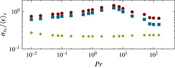
while the kinetic energy sink and flux do. This observation can be seen more quantitatively in figure 10, which shows that the vertical source inhomogeneity is small for all
 $\mathit{Pr}$
, whereas the vertical dissipation inhomogeneity and the redistribution vary as a function of the Prandtl number. It is observed that, apart from a constant prefactor in the amplitude, the r.m.s. redistribution shows a similar Prandtl number dependence to the vertical dissipation inhomogeneity: both quantities increase with
 $\mathit{Pr}$
for low Prandtl numbers, form a maximum at
 $\mathit{Pr}\approx 5$
and then decrease again for high Prandtl numbers. These findings reveal that the redistribution is related to the inhomogeneity of the dissipation.
Vertical inhomogeneities of the profiles of the dissipation and the source, and the redistribution by flux, measured by the vertical standard deviation
 ${\it\sigma}_{x_{3}}$
(6.1) of the respective profile, versus the Prandtl number. The blue squares denote the vertical dissipation inhomogeneity
 $({\it\sigma}_{x_{3}}({\it\epsilon}))$
while the green diamonds denote the vertical source inhomogeneity
 $({\it\sigma}_{x_{3}}(S))$
and the red dots indicate the r.m.s. redistribution by flux
 $({\it\sigma}_{x_{3}}(\partial _{3}J_{3}))$
.

The non-monotonic
 $\mathit{Pr}$
dependence of the dissipation with a maximum at moderate Prandtl number suggests a competition of two effects: the decreasing transport of kinetic energy with decreasing
 $\mathit{Pr}$
for low Prandtl numbers might be the consequence of a homogenisation due to increased bulk turbulence. This seems plausible in view of the fact that the Reynolds number increases for decreasing Prandtl number, and is consistent with a bulk-dominated flow, as predicted by Grossmann & Lohse (Reference Grossmann and Lohse2000). The decreasing transport for high Prandtl number is likely to be caused by a smoothing of the velocity field due to diffusion at high
 $\mathit{Pr}$
, which leads to a more homogeneous dissipation profile. This process becomes dominant at approximately
 $\mathit{Pr}\approx 5$
, and obviously outweighs the effect of enhanced dissipation near the walls (Grossmann & Lohse Reference Grossmann and Lohse2000).
6.3. Redistributions by individual fluxes
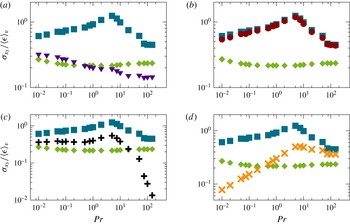
For a more detailed analysis of the Prandtl number dependence of the dissipation, figure 11 shows the r.m.s. redistributions by the individual fluxes. It is observed that, apart from the buoyancy-pressure flux, the r.m.s. redistributions by all fluxes separate the observed parameter space into two regimes. The transition between these regimes takes place at
 $\mathit{Pr}\approx 5$
where the vertical dissipation inhomogeneity also exhibits a maximum.
Root-mean-square redistributions by different fluxes along with the vertical source and dissipation inhomogeneities, measured by the vertical standard deviation
 ${\it\sigma}_{x_{3}}$
(6.1) of the respective profile, versus the Prandtl number. The blue squares denote the vertical dissipation inhomogeneity
 $({\it\sigma}_{x_{3}}({\it\epsilon}))$
while the green diamonds denote the vertical source inhomogeneity
 $({\it\sigma}_{x_{3}}(S))$
. The purple triangles indicate the redistribution by buoyancy-pressure flux in (a)
 $({\it\sigma}_{x_{3}}(\partial _{3}J_{3}^{buo}))$
, the red dots indicate the redistribution by viscous shear flux in (b)
 $({\it\sigma}_{x_{3}}(\partial _{3}J_{3}^{shear}))$
, the black crosses indicate the redistribution by advective flux in (c)
 $({\it\sigma}_{x_{3}}(\partial _{x_{3}}J_{3}^{adv}))$
and the orange crosses denote the redistribution by the viscous normal flux in (d)
 $({\it\sigma}_{x_{3}}(\partial _{3}J_{3}^{norm}))$
.

Similarly to the layer thicknesses, the redistribution by buoyancy pressure (see figure 11
a) is related to the kinetic energy source. Both the amplitudes as well as the Prandtl number dependence are broadly comparable to the vertical source inhomogeneity. The r.m.s. redistribution decreases for increasing
 $\mathit{Pr}$
throughout the parameter range covered by our study.
A common view of describing convection for different Prandtl numbers is to assume that advection plays a major role for low Prandtl numbers whereas high Prandtl numbers are characterised by viscous effects (Grossmann & Lohse Reference Grossmann and Lohse2000; Breuer et al.
Reference Breuer, Wessling, Schmalzl and Hansen2004). The redistributions by advection (figure 11
c) and by normal stress (figure 11
d) support these assumptions. In the low-Prandtl-number regime the normal-stress redistribution decreases monotonically with decreasing
 $\mathit{Pr}$
, whereas the advective redistribution saturates for small
 $\mathit{Pr}$
. In the high-Prandtl-number regime the normal-stress redistribution saturates at high values whereas the advective redistribution decreases rapidly with increasing
 $\mathit{Pr}$
. The dominance of viscous effects for high
 $\mathit{Pr}$
is often related to a growing velocity boundary layer (Grossmann & Lohse Reference Grossmann and Lohse2000). In this case, however, the kinetic energy transport by viscous effects can be related to normal stresses and not to shear stresses and is therefore not associated with boundary layer processes.
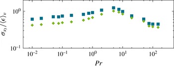
Root-mean-square redistribution of kinetic energy by the sum of advective flux and normal-stress flux along with the vertical dissipation inhomogeneity, measured by the vertical standard deviation
 ${\it\sigma}_{x_{3}}$
(6.1) of the respective profile, versus the Prandtl number. The blue squares denote the vertical inhomogeneity of the dissipation profile (
 ${\it\sigma}_{x_{3}}({\it\epsilon})$
) while the green diamonds denote the redistribution by the flux
 $({\it\sigma}_{x_{3}}(\partial _{3}J_{3}^{adv+norm}))$
.

Classical boundary layer processes only become dominant closer to the walls. In fact, it is observed that the shear-stress flux layer is approximately the same size as the velocity boundary layer (cf. figure 9). The r.m.s. redistribution by shear stress (figure 11
b) displays a nearly identical Prandtl number dependence to the vertical dissipation inhomogeneity. These similarities may be related to the balance of both quantities at the boundaries. The identical Prandtl number dependences of the redistribution by shear and the vertical dissipation inhomogeneity might naively be interpreted as a strong influence of the shear stress on the kinetic energy dissipation profile. However, the redistribution by shear stress takes place much closer to the wall than all the other redistributions (cf. figure 9). This points out that advection and normal stresses redistribute kinetic energy from the source layer into the dissipation layer, from where it is further redistributed into the boundary layer by shear stresses. Because the shear-stress redistribution follows the vertical dissipation inhomogeneity for all Prandtl numbers, the shear stress cannot be associated with the decreasing vertical dissipation inhomogeneity in only one of the two
 $\mathit{Pr}$
regimes.
The opposing Prandtl number dependence of the advective and normal-stress redistributions indicates two competing Prandtl number dependences which may result in a maximum at moderate
 $\mathit{Pr}$
. This becomes clearer by analysing the redistribution by the sum of both fluxes, which can be seen in figure 12 along with the vertical kinetic energy dissipation inhomogeneity. It can be seen that the redistribution by the sum of both fluxes indeed displays a Prandtl number dependence similar to the vertical inhomogeneity of the dissipation profile. Only for low Prandtl numbers does an approximately constant prefactor in the amplitude distinguish the redistribution and the vertical dissipation inhomogeneity, which appears to be caused by the increasing influence of the kinetic energy redistribution by buoyancy pressure. In summary, in order to explain the dissipation profile, both the shear-stress flux close to the boundary and the combined effect of advective and normal-stress flux need to be considered.
7. Summary and discussion
In this work we have extensively analysed the contributions to the kinetic energy budget in Rayleigh–Bénard convection for a range of Prandtl numbers at a fixed Rayleigh number. The results presented allow us to draw a comprehensive picture of kinetic energy transport. On a very general level, we observe that the kinetic energy is produced in the central region where the temperature field is well mixed, from where it is transported outwards and dissipated near the walls. This is consistent with the observations of earlier studies by Deardorff & Willis (Reference Deardorff and Willis1967) and Kerr (Reference Kerr2001). It is also intuitive because fluid is accelerated due to buoyancy forces in the bulk, and decelerated on approaching the boundaries of the volume.
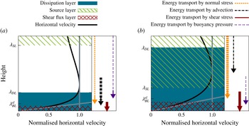
On a more detailed level, our work provides a comprehensive view of the physical processes involved in transporting the kinetic energy from the bulk towards the walls. The dynamics is found to be surprisingly rich and exhibits a pronounced Prandtl number dependence. The investigated Prandtl number range can be separated into two characteristic regimes, corresponding to high and low Prandtl numbers. Figure 13 shows a schematic sketch of the near-wall region for two exemplary Prandtl numbers (
 $\mathit{Pr}=0.1$
and
 $\mathit{Pr}=100$
). Regions of enhanced dissipation (blue solid areas) and enhanced production (green shaded areas) of kinetic energy are shown. The arrows indicate the kinetic energy fluxes, each of which is caused by a different process. The arrows point from the height of maximal removal to the height of maximal accumulation of kinetic energy, with bold lines indicating dominant contributions.
Sketch of the different layers of the kinetic energy balance along with the profile of the r.m.s. of the horizontal velocity normalised by its maximum for
 $\mathit{Pr}=0.1$
(a) and
 $\mathit{Pr}=100$
(b). Additionally, the spatial redistribution of kinetic energy is represented schematically by the arrows on the right margin. The starting points of these arrows indicate the height of maximal removal of kinetic energy whereas the endpoints indicate the height of maximal accumulation of kinetic energy. The broad arrows denote the dominant flux processes.

Perhaps the most striking feature is that the dissipation and source regions are spatially separated for low Prandtl numbers, whereas they penetrate each other for high Prandtl numbers. This spatial overlap of the source and dissipation regions is found to be crucial in allowing the boundary region to dominate the overall dissipation at high
 $\mathit{Pr}$
(Grossmann & Lohse Reference Grossmann and Lohse2000; Petschel et al.
Reference Petschel, Stellmach, Wilczek, Lülff and Hansen2013). The kinetic energy fluxes alone are too weak to balance the dissipative kinetic energy losses within this region. For low Prandtl numbers, the source and dissipation regions do not overlap, such that the dissipative losses have to be balanced almost entirely by fluxes transporting kinetic energy over the spatial gap between the source and dissipation regions. These fluxes are mainly accomplished by advection. A strong kinetic energy flux from the bulk to the boundary region is also observed at large
 $\mathit{Pr}$
. Instead of advection, normal viscous stresses dominate the transport in this case. Interestingly, for all Prandtl numbers, viscous shear stresses merely redistribute kinetic energy within the dissipative region and play a crucial role in balancing the viscous dissipation on the rigid walls.
In order to put these results on a more quantitative footing, we proposed exact layer definitions reflecting the above picture. Extending the concept of dissipation layers, introduced earlier by Petschel et al. (Reference Petschel, Stellmach, Wilczek, Lülff and Hansen2013), to source layers and flux layers, our work suggests a decomposition of the convective domain into several distinct sublayers, each characterised by different physical processes at work, either producing, dissipating or transporting kinetic energy. These new layers prove to be useful in contextualising previous work relying on specific definitions of mechanical boundary layers.
Popular boundary layer definitions include the so-called slope method or are based on the maximum of the horizontal velocity profile. While originally introduced heuristically, our work reveals that they are deeply connected to the kinetic energy transport. The edge of the maximum boundary layer is reinterpreted as the location from where on viscous shear stresses begin to transport kinetic energy towards the boundary. In contrast, the edge of a boundary layer defined by the slope method is found to mark the location where viscous shear stresses begin to accumulate kinetic energy close to the wall. Both definitions, however, fail to correctly represent the region of enhanced dissipation, in contrast to the dissipation layer introduced by Petschel et al. (Reference Petschel, Stellmach, Wilczek, Lülff and Hansen2013). This is in line with recent results by Scheel & Schumacher (Reference Scheel and Schumacher2014), who showed that boundary layers determined by the slope method and dissipation layers exhibit opposite Rayleigh number trends.
For the current work we have considered a wide range of Prandtl numbers for a fixed moderate Rayleigh number. In the future, it would also be very interesting to see how our observations vary when the Rayleigh number is increased. Such a study is numerically challenging, as high spatial resolutions are needed to resolve the flow in the low-Prandtl-number regime (cf. figure 1 d).