


%20--%3e%3c!DOCTYPE%20svg%20PUBLIC%20'-//W3C//DTD%20SVG%201.0//EN'%20'http://www.w3.org/TR/2001/REC-SVG-20010904/DTD/svg10.dtd'%3e%3csvg%20version='1.0'%20id='Layer_1'%20xmlns='http://www.w3.org/2000/svg'%20xmlns:xlink='http://www.w3.org/1999/xlink'%20x='0px'%20y='0px'%20width='64px'%20height='64px'%20viewBox='5.5%20-3.5%2064%2064'%20enable-background='new%205.5%20-3.5%2064%2064'%20xml:space='preserve'%3e%3cg%3e%3ccircle%20fill='%23FFFFFF'%20fill-opacity='0'%20cx='37.785'%20cy='28.501'%20r='28.836'/%3e%3cpath%20fill='%23595959'%20d='M37.441-3.5c8.951,0,16.572,3.125,22.857,9.372c3.008,3.009,5.295,6.448,6.857,10.314%20c1.561,3.867,2.344,7.971,2.344,12.314c0,4.381-0.773,8.486-2.314,12.313c-1.543,3.828-3.82,7.21-6.828,10.143%20c-3.123,3.085-6.666,5.448-10.629,7.086c-3.961,1.638-8.057,2.457-12.285,2.457s-8.276-0.808-12.143-2.429%20c-3.866-1.618-7.333-3.961-10.4-7.027c-3.067-3.066-5.4-6.524-7-10.372S5.5,32.767,5.5,28.5c0-4.229,0.809-8.295,2.428-12.2%20c1.619-3.905,3.972-7.4,7.057-10.486C21.08-0.394,28.565-3.5,37.441-3.5z%20M37.557,2.272c-7.314,0-13.467,2.553-18.458,7.657%20c-2.515,2.553-4.448,5.419-5.8,8.6c-1.354,3.181-2.029,6.505-2.029,9.972c0,3.429,0.675,6.734,2.029,9.913%20c1.353,3.183,3.285,6.021,5.8,8.516c2.514,2.496,5.351,4.399,8.515,5.715c3.161,1.314,6.476,1.971,9.943,1.971%20c3.428,0,6.75-0.665,9.973-1.999c3.219-1.335,6.121-3.257,8.713-5.771c4.99-4.876,7.484-10.99,7.484-18.344%20c0-3.543-0.648-6.895-1.943-10.057c-1.293-3.162-3.18-5.98-5.654-8.458C50.984,4.844,44.795,2.272,37.557,2.272z%20M37.156,23.187%20l-4.287,2.229c-0.458-0.951-1.019-1.619-1.685-2c-0.667-0.38-1.286-0.571-1.858-0.571c-2.856,0-4.286,1.885-4.286,5.657%20c0,1.714,0.362,3.084,1.085,4.113c0.724,1.029,1.791,1.544,3.201,1.544c1.867,0,3.181-0.915,3.944-2.743l3.942,2%20c-0.838,1.563-2,2.791-3.486,3.686c-1.484,0.896-3.123,1.343-4.914,1.343c-2.857,0-5.163-0.875-6.915-2.629%20c-1.752-1.752-2.628-4.19-2.628-7.313c0-3.048,0.886-5.466,2.657-7.257c1.771-1.79,4.009-2.686,6.715-2.686%20C32.604,18.558,35.441,20.101,37.156,23.187z%20M55.613,23.187l-4.229,2.229c-0.457-0.951-1.02-1.619-1.686-2%20c-0.668-0.38-1.307-0.571-1.914-0.571c-2.857,0-4.287,1.885-4.287,5.657c0,1.714,0.363,3.084,1.086,4.113%20c0.723,1.029,1.789,1.544,3.201,1.544c1.865,0,3.18-0.915,3.941-2.743l4,2c-0.875,1.563-2.057,2.791-3.541,3.686%20c-1.486,0.896-3.105,1.343-4.857,1.343c-2.896,0-5.209-0.875-6.941-2.629c-1.736-1.752-2.602-4.19-2.602-7.313%20c0-3.048,0.885-5.466,2.658-7.257c1.77-1.79,4.008-2.686,6.713-2.686C51.117,18.558,53.938,20.101,55.613,23.187z'/%3e%3c/g%3e%3c/svg%3e)
%20--%3e%3c!DOCTYPE%20svg%20PUBLIC%20'-//W3C//DTD%20SVG%201.0//EN'%20'http://www.w3.org/TR/2001/REC-SVG-20010904/DTD/svg10.dtd'%3e%3csvg%20version='1.0'%20id='Layer_1'%20xmlns='http://www.w3.org/2000/svg'%20xmlns:xlink='http://www.w3.org/1999/xlink'%20x='0px'%20y='0px'%20width='64px'%20height='64px'%20viewBox='5.5%20-3.5%2064%2064'%20enable-background='new%205.5%20-3.5%2064%2064'%20xml:space='preserve'%3e%3cg%3e%3ccircle%20fill='%23FFFFFF'%20fill-opacity='0'%20cx='37.637'%20cy='28.806'%20r='28.276'/%3e%3cg%3e%3cpath%20fill='%23595959'%20d='M37.443-3.5c8.988,0,16.57,3.085,22.742,9.257C66.393,11.967,69.5,19.548,69.5,28.5c0,8.991-3.049,16.476-9.145,22.456%20C53.879,57.319,46.242,60.5,37.443,60.5c-8.649,0-16.153-3.144-22.514-9.43C8.644,44.784,5.5,37.262,5.5,28.5%20c0-8.761,3.144-16.342,9.429-22.742C21.101-0.415,28.604-3.5,37.443-3.5z%20M37.557,2.272c-7.276,0-13.428,2.553-18.457,7.657%20c-5.22,5.334-7.829,11.525-7.829,18.572c0,7.086,2.59,13.22,7.77,18.398c5.181,5.182,11.352,7.771,18.514,7.771%20c7.123,0,13.334-2.607,18.629-7.828c5.029-4.838,7.543-10.952,7.543-18.343c0-7.276-2.553-13.465-7.656-18.571%20C50.967,4.824,44.795,2.272,37.557,2.272z%20M46.129,20.557v13.085h-3.656v15.542h-9.944V33.643h-3.656V20.557%20c0-0.572,0.2-1.057,0.599-1.457c0.401-0.399,0.887-0.6,1.457-0.6h13.144c0.533,0,1.01,0.2,1.428,0.6%20C45.918,19.5,46.129,19.986,46.129,20.557z%20M33.042,12.329c0-3.008,1.485-4.514,4.458-4.514s4.457,1.504,4.457,4.514%20c0,2.971-1.486,4.457-4.457,4.457S33.042,15.3,33.042,12.329z'/%3e%3c/g%3e%3c/g%3e%3c/svg%3e)
1. Introduction
The recent release of the fourth Gravitational-Wave Transient Catalog (GWTC-4) has brought the number of detected binary black hole (BBH) mergers to over 150 (The LIGO-Virgo-KAGRA Collaboration 2025), affirming the presence of a
 $M_1\sim35\,\mathrm{M}_\odot$
peak for BBHs. Although one of the most robustly inferred features of gravitational-wave (GW) data, the
 $\sim35\,\mathrm{M}_\odot$
peak still lacks a satisfactory explanation (e.g., Roy et al. Reference Roy, van Son and Farr2025, and references therein).
We explore one possible formation channel: chemically homogeneously evolving (CHE) stars. Characterized by rapid rotation rates and low metallicities, these stars have been proposed to develop meridional currents that efficiently mix material throughout the envelope (e.g., Yoon and Langer Reference Yoon and Langer2005; Yoon et al. Reference Yoon, Langer and Norman2006). As a result, they become He-enriched on the surface by the end of the Main Sequence (MS), and remain compact throughout their lives. Because the necessary rotation is assumed to develop from tidal locking in tight binaries, these factors make them good potential BBH progenitors (Mandel and de Mink Reference Mandel and de Mink2016; Marchant et al. Reference Marchant, Langer, Podsiadlowski, Tauris and Moriya2016). They are furthermore expected to lead to more massive BBHs (
 $M_1\gtrsim20\,\mathrm{M}_\odot$
) because rotational mixing is only effective in more massive, radiation-dominated stars (Hastings et al. Reference Hastings, Langer and Koenigsberger2020), and because their compactness avoids mass transfer episodes, potentially allowing them to retain a larger fraction of their initial mass. Finally, CHE mostly forms equal-mass binaries (though mass ratios as low as
 $q\approx0.7$
might occur in
 $\sim20\%$
of systems, see Marchant et al. Reference Marchant, Langer, Podsiadlowski, Tauris and Moriya2016; Hastings et al. Reference Hastings, Langer and Koenigsberger2020), which is also in line with recent findings on the
 $M_1\sim35\,\mathrm{M}_\odot$
peak (Roy et al. Reference Roy, van Son and Farr2025; Banagiri et al. Reference Banagiri, Thrane and Lasky2025).
2. MESA setup
We run grids of CHE star models with version 23.04.1 of the 1D stellar structure code Modules for Experiments in Stellar Astrophysics (MESA, Paxton et al. Reference Paxton, Bildsten, Dotter, Herwig, Lesaffre and Timmes2011; Paxton et al. Reference Paxton, Cantiello, Arras, Bildsten, Brown, Dotter, Mankovich, Montgomery, Stello, Timmes and Townsend2013; Paxton et al. Reference Paxton, Marchant, Schwab, Bauer, Bildsten, Cantiello, Dessart, Farmer, Hu, Langer, Townsend, Townsley and Timmes2015; Paxton et al. Reference Paxton, Schwab, Bauer, Bildsten, Blinnikov, Duffell, Farmer, Goldberg, Marchant, Sorokina, Thoul, Townsend and Timmes2018; Paxton et al. Reference Paxton, Smolec, Schwab, Gautschy, Bildsten, Cantiello, Dotter, Farmer, Goldberg, Jermyn, Kanbur, Marchant, Thoul, Townsend, Wolf, Zhang and Timmes2019; Jermyn et al. Reference Jermyn, Bauer, Schwab, Farmer, Ball, Bellinger, Dotter, Joyce, Marchant, Mombarg, Wolf, Sunny Wong, Cinquegrana, Farrell, Smolec, Thoul, Cantiello, Herwig, Toloza, Bildsten, Townsend and Timmes2023). We build our models based on the inlists and extra routines from Gottlieb et al. (Reference Gottlieb, Renzo, Metzger, Goldberg and Cantiello2024), with the
 $\sigma=0$
 $^{12}\mathrm{C}(\alpha,\gamma)^{16}\mathrm{O}$
reaction rate from deBoer et al. (Reference deBoer, Görres, Wiescher, Azuma, Best, Brune, Fields, Jones, Pignatari, Sayre, Smith, Timmes and Uberseder2017) as our fiducial assumption. Besides varying mass, initial spin periods and metallicities, we build an updated wind scheme, with the minimum between Björklund et al. (Reference Björklund, Sundqvist, Singh, Puls and Najarro2023) and Krtika et al. (2024) for thin (OB) winds; Vink et al. (Reference Vink, Muijres, Anthonisse, de Koter, Gräfener and Langer2011) for thick (very massive star, VMS) He-poor winds; and the minimum between Sander and Vink (Reference Sander and Vink2020) (with the Sander et al. Reference Sander, Lefever, Poniatowski, Ramachandran, Sabhahit and Vink2023, temperature correction) and Vink (Reference Vink2017) for thick (Wolf-Rayet, WR) He-rich winds. We transition to thick He-poor winds following the framework by Sabhahit et al. (Reference Sabhahit, Vink, Sander and Higgins2023), and to He-rich winds by interpolating between He-poor (either thin OB or thick VMS) and He-rich WR winds within the
 $Y_\mathrm{surf}=0.4-0.7$
range. Finally, we adopt rotation-enhanced mass-loss following Heger et al. (Reference Heger, Langer and Woosley2000).
For simplicity, we run only single stellar evolution models, which we find to allow for CHE for a wide range of zero-age MS (ZAMS) masses and spins. We emulate binary evolution by assuming
 $q=1$
, tidal synchronization at ZAMS (de Mink et al. Reference de Mink, Cantiello, Langer, Pols, Brott and Yoon2009) and Jeans mode mass loss. Models are run up to core carbon depletion, after which point the star is not expected to lose any significant amount of mass or angular momentum (AM). We define CHE as maintaining
 $Y_\mathrm{surf}/Y_\mathrm{center}\geq0.7$
throughout the MS, and stop any runs that violate this condition or lead into a stellar merger at ZAMS by overflow through the second Lagrangian point (following Marchant et al. Reference Marchant, Langer, Podsiadlowski, Tauris and Moriya2016).
Our model grid consists of 20 values of
 $M_{\mathrm{ZAMS}}$
, uniformly sampled with step
 $10\,\mathrm{M}_\odot$
between
 $20-120\,\mathrm{M}_\odot$
, and with step
 $20\,\mathrm{M}_\odot$
between
 $120-300\,\mathrm{M}_\odot$
; and 36 values of
 $P_{\mathrm{ZAMS}}$
, with step
 $0.05\,\mathrm{d}$
between
 $0.35-0.90\,\mathrm{d}$
, step
 $0.1\,\mathrm{d}$
between
 $0.90-2.60\,\mathrm{d}$
, and step
 $0.2\,\mathrm{d}$
between
 $2.60-4.00\,\mathrm{d}$
. Each of the 720 models is evolved for 9 metallicities,
 $Z/{\mathrm{Z}_\odot}=1/100,1/50,1/20,1/10,1/5,0.4,0.6,0.8,1.0$
, bringing the total to 6480 models.
Next, we use these MESA models to estimate a population of merging binary black holes. To this end, we fit three-dimensional linear interpolators on
 $M_{\mathrm{ZAMS}}$
,
 $P_{\mathrm{ZAMS}}$
and Z over our MESA grids, and re-draw
 $M_{\mathrm{ZAMS}}$
from a Kroupa (Reference Kroupa2001) IMF, and
 $P_{\mathrm{ZAMS}}$
from a log-uniform distribution. Unless stated otherwise, metallicities are re-drawn from the redshift-dependent skewed-Gaussian distribution from van Son et al. (Reference van Son, de Mink, Chruliska, Conroy, Pakmor and Hernquist2023). We compute merger rates from large interpolated populations with a MESA-adapted version of CosmicIntegrator, part of the post-processing suite of the COMPAS binary population synthesis code (Neijssel et al. Reference Neijssel, Vigna-Gómez, Stevenson, Barrett, Gaebel, Broekgaarden, de Mink, Szécsi, Vinciguerra and Mandel2019; Riley et al. Reference Riley, Mandel, Marchant, Butler, Nathaniel, Neijssel, Shortt and Vigna-Gómez2021).
3. The BBH yield from CHE at fixed metallicity
From our Fiducial model grid, we find that the minimum mass at ZAMS for which CHE occurs is
 $\sim30\,\mathrm{M}_\odot$
for metallicities below
 $0.2\,{\mathrm{Z}_\odot}$
, and
 $\sim50\,\mathrm{M}_\odot$
for
 $Z\geq0.2$
. Fig. 1 shows the resulting final primary mass distribution for six different metallicity ranges, without filtering for delay time, from an interpolated
 $\sim10^8$
binary population following a log-uniform metallicity distribution. The effect of increasing wind mass-loss with metallicity is immediately evident, with the high metallicity (
 $-0.3\leq\log Z/{\mathrm{Z}_\odot}\lt0$
) range producing a sharp peak at
 $\sim10\,\mathrm{M}_\odot$
, while the low metallicity (
 $-2\leq\log Z/{\mathrm{Z}_\odot}\lt-1.7$
) range produces masses between
 $\sim35\,\mathrm{M}_\odot$
and
 $\sim95\,\mathrm{M}_\odot$
, with a modest pile-up at the upper end. Conspicuously, all
 $\log Z/{\mathrm{Z}_\odot}\gt-0.7$
metallicities produce either a peak or a sharp cut-off around
 $\sim35\,\mathrm{M}_\odot$
(black vertical line in Fig. 1).
Final mass distribution from an interpolated population of
 $10^8$
binaries over different metallicity intervals, for a population generated following the Kroupa (Reference Kroupa2001) IMF, a log-uniform orbital period distribution and a log-uniform metallicity distribution. The solid vertical line indicates
 $M_\mathrm{f}=35\,\mathrm{M}_\odot$
.

Two main effects shape the distribution in Fig. 1. First is the interplay between the minimal ZAMS mass required for CHE,
 $m_{\mathrm{CHE}}^{\mathrm{min}}\approx30\,\mathrm{M}_\odot$
, at low metallicities, and the Kroupa (Reference Kroupa2001) IMF, which favors lower masses. In other words, the initial mass function of CHE stars is itself peaked slightly above the lower edge of the window, i.e.,
 $\sim35\,\mathrm{M}_\odot$
. In the absence of mass loss, this means most stars will have a final mass of
 $\sim35\,\mathrm{M}_\odot$
, which leads to the lowest metallicities in Fig. 1 seeing their final masses cut off around that value.
The second effect is the strong wind mass-loss from WR and VMS winds. VMS winds dominate mass-loss at the lowest metallicities, setting the maximum final mass of
 $\sim90\,\mathrm{M}_\odot$
visible in Fig. 1. At intermediate metallicities, WR (He-rich) winds lead to significant mass-loss even at
 $\lt100\,\mathrm{M}_\odot$
, narrowing the distribution towards the minimum progenitor mass of
 $\sim35\,\mathrm{M}_\odot$
, where mass-loss becomes weak enough to create a pile-up. At the highest metallicities, the CHE window closes at
 $M_\mathrm{ZAMS}\sim50\,\mathrm{M}_\odot$
, but mass-loss is so intense that the distribution shifts to create a narrow peak at final masses as low as
 $\sim10\,\mathrm{M}_\odot$
.
4. Merger rates
We draw a new
 $\sim10^8$
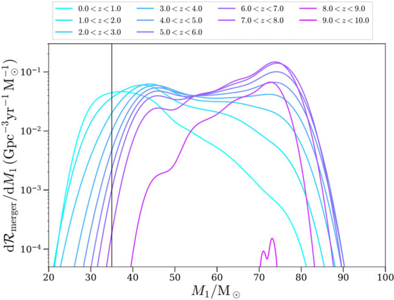
binary interpolated population, this time sampling from the van Son et al. (Reference van Son, de Mink, Chruliska, Conroy, Pakmor and Hernquist2023) metallicity distribution. Fig. 2 shows the resulting BBH merger rates. This demonstrates that our fiducial model peaks at
 $\sim35\,\mathrm{M}_\odot$
for low redshifts (
 $0 \lt z \lt 1$
). This peak shifts to higher masses with redshift. This is the result of a mass-metallicity-delay time relation: lower metallicities, with weaker winds, favor greater masses and shorter delay times. Thus, the most massive mergers form early (higher redshift) and merge quickly, while the least massive mergers form later (lower redshift) and merge later.
Merger rates over mass, for different redshift bins, for an interpolated
 $10^8$
binary population, drawn from the Kroupa (Reference Kroupa2001) IMF, a log-uniform orbital period distribution and the metallicity distribution by van Son et al. (Reference van Son, de Mink, Chruliska, Conroy, Pakmor and Hernquist2023). The solid vertical line indicates
 $M_\mathrm{1}=35\,\mathrm{M}_\odot$
.

In summary, we find that the CHE channel creates a low-redshift
 $\sim35\,\mathrm{M}_\odot$
peak hailing from the interplay between the IMF and WR winds; and a high-redshift
 $\sim90\,\mathrm{M}_\odot$
peak hailing from VMS winds. The distribution shifts smoothly from one to the other with increasing redshift. We note, however, that while our current simulations produce a reasonable match for the peak location, our merger rates are much broader in
 $M_1$
than what is supported (see Roy et al. Reference Roy, van Son and Farr2025). We conclude that our results suggest how CHE might explain a feature at
 $35\mathrm{M}_\odot$
, but that our particular assumptions are not fully compatible with observations.
Spins
Another important constraint is that the
 $\sim35\,\mathrm{M}_\odot$
mergers are consistent with slowly-spinning,
 $\chi\lt0.1$
BHs (Roy et al. Reference Roy, van Son and Farr2025). We find our Fiducial grid, which assumes the traditional Tayler-Spruit (TS) dynamo (Spruit Reference Spruit2002), to exclusively result in
 $\chi\gt1$
cores. These are likely to lead to a collapsar and GRB launch, which have been found to be efficient at halting BH spins, but also at unbinding up to
 $\sim90\%$
of a WR progenitor’s mass (e.g. Gottlieb et al. Reference Gottlieb, Liska, Tchekhovskoy, Bromberg, Lalakos, Giannios and Mösta2022), which would rule out CHE as the peak progenitor. We re-run a small subset of models with the Fuller and Lu (Reference Fuller and Lu2022) AM transport prescription, which we find to exclusively produce
 $\chi\lt0.01$
cores. Such a situation allows for the production of the
 $\sim35\,\mathrm{M}_\odot$
peak. However, we stress that this would eliminate CHE stars as GRB progenitors. Whether AM transport in CHE stars corresponds to either model or has a more moderate efficiency remains unclear, and the problem of spins is left to future work.
5. Conclusions
We have mapped out the conditions under which CHE could be responsible for the
 $\sim35\,\mathrm{M}_\odot$
peak. In the absence of mass transfer, CHE results in a (thick) wind-dominated BBH merger formation channel. Crucially, CHE allows thick WR winds to affect lower progenitor masses, for which VMS winds are not activated, without mass transfer. The bump in merger rates is a reflection of the minimum mass for CHE, at which winds become negligible. We assume the BH mass directly tracks the final progenitor mass. The efficiency of rotational mixing and the nature of CHE star mass-loss are thus the most critical assumptions for CHE. Determining whether CHE stars can simultaneously satisfy the mass and spin constraints required to match the
 $M_1\sim35\,\mathrm{M}_\odot$
peak observed in BBH mergers, while also accounting for GRBs, will require further study, leaving CHE as an exciting topic at the intersection between GWs, GRBs and WRs.

 108
 Mf=35M⊙
 108
 M1=35M⊙

 Open access

