1 Introduction
Irreversible mixing is ubiquitous in environmental and industrial flows, and is a critical mechanism for ocean and atmosphere dynamics as well as a crucial element in many manufacturing processes, occurring on various length and time scales. Consequently, there has been great interest in understanding, quantifying and finally improving the mixing properties of a vast range of flows, whether to prevent or, alternatively to enhance, homogenisation, notably through the triggering of hydrodynamic instabilities. In particular recently, maximisation of the (transient) perturbation kinetic energy, associated with the inherent non-normality of the linearised Navier–Stokes operator, has been used as a convenient proxy for optimising mixing efficiency without requiring a direct assessment of well-mixedness, which in a real sense is both an essentially nonlinear and diffusive phenomenon, requiring as it does an (irreversible) modification of an initial base or background scalar distribution.
The fundamental mathematical hypothesis underlying this approach (see e.g. Aamo, Krstic & Bewley (Reference Aamo, Krstic and Bewley2003), Balogh, Aamo & Krstic (Reference Balogh, Aamo and Krstic2005)) is that the ‘best’ way (ultimately) to mix a scalar in a fluid flow is to encourage flow instabilities or transiently growing perturbations, presumably eventually triggering nonlinearities which would prevent disturbances from fading away, thus ensuring scalar homogenisation. On the other hand, recently developed mathematical tools, in particular what we refer to here as the direct-adjoint-looping (DAL) method (see § 2.2.2 and references therein) have provided a new algorithmic approach for inherently nonlinear optimisation of a chosen quantity of interest, which can be an appropriately chosen direct measure of mixing.
Quantifying mixing is however not always an immediately straightforward task, and the choice of a particular measure can have implications for the optimal mixing strategy within a finite time horizon. Let us consider
 $\unicode[STIX]{x1D70C}(\boldsymbol{x},t)$
to be a scalar field with diffusivity
 $\unicode[STIX]{x1D705}$
in a fluid with velocity field
 $\boldsymbol{U}(\boldsymbol{x},t)$
. If there are no sources or sinks in the domain,
 $\unicode[STIX]{x1D6FA}$
, of interest,
 $\unicode[STIX]{x1D70C}$
satisfies the advection–diffusion equation
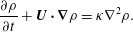 $$\begin{eqnarray}\frac{\unicode[STIX]{x2202}\unicode[STIX]{x1D70C}}{\unicode[STIX]{x2202}t}+\boldsymbol{U}\boldsymbol{\cdot }\unicode[STIX]{x1D735}\unicode[STIX]{x1D70C}=\unicode[STIX]{x1D705}\unicode[STIX]{x1D6FB}^{2}\unicode[STIX]{x1D70C}.\end{eqnarray}$$
Without loss of generality, we may assume that
 $\unicode[STIX]{x1D70C}$
has spatial mean zero. Its variance
 $\mathscr{V}=\Vert \unicode[STIX]{x1D70C}\Vert _{2}^{2}$
, where the appropriately normalised
 $L_{2}$
-norm is defined as
 $\Vert X\Vert _{2}^{2}=(1/V_{\unicode[STIX]{x1D6FA}})\int _{\unicode[STIX]{x1D6FA}}|X|^{2}\,\text{d}\unicode[STIX]{x1D6FA}$
, provides a natural and meaningful measure of the mixedness of the fluid as it quantifies the deviation from the (zero) scalar spatial mean over the domain
 $\unicode[STIX]{x1D6FA}$
of volume
 $V_{\unicode[STIX]{x1D6FA}}$
. The evolution equation for the variance is readily derived from (1.1):
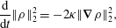 $$\begin{eqnarray}\frac{\text{d}}{\text{d}t}\Vert \unicode[STIX]{x1D70C}\Vert _{2}^{2}=-2\unicode[STIX]{x1D705}\Vert \unicode[STIX]{x1D735}\unicode[STIX]{x1D70C}\Vert _{2}^{2},\end{eqnarray}$$
indicating that the variance monotonically decreases toward zero, with a decay rate determined exclusively by the diffusivity. From a mixing optimisation point of view, a first issue arising from this equation is that the variance decay rate depends only implicitly on the velocity field, through the velocity field inducing high gradients in the scalar field. Indeed, efficient mixing occurs through the (intermediate time) creation of strong local gradients, which are then ultimately smoothed by diffusion at small scale. A second practical issue is that (1.2) is not useful to describe homogenisation in the theoretical limit of pure ‘stirring’ i.e. as
 $\unicode[STIX]{x1D705}\rightarrow 0$
.
Specifically to overcome this issue, Mathew, Mezic & Petzold (Reference Mathew, Mezic and Petzold2005) and Doering & Thiffeault (Reference Doering and Thiffeault2006) have introduced and generalised what are now commonly referred to as mix-norms, namely Sobolev norms of negative (possibly fractional) index (see Thiffeault (Reference Thiffeault2012) for a valuable review of mix-norms). These measures downplay the contribution of small scales by comparison to large scales, and so scalar distributions with small values of a mix-norm can reasonably be thought to be (at least) approaching well-mixedness. Use of such mix-norms has already proved useful in a variety of mixing optimisation problems where a passive scalar is advected by a pre-determined velocity field, with or without sources (see for example Mathew et al. (Reference Mathew, Mezic, Grivopoulos, Vaidya and Petzold2007), Thiffeault & Pavliotis (Reference Thiffeault and Pavliotis2008), Lin, Thiffeault & Doering (Reference Lin, Thiffeault and Doering2010)). Here, we will restrict our attention to the specific (particularly computationally attractive) mix-norm for a zero spatial mean quantity
 $\unicode[STIX]{x1D70C}$
:
 $$\begin{eqnarray}\mathscr{M}=\Vert \unicode[STIX]{x1D6FB}^{-1}\unicode[STIX]{x1D70C}\Vert _{2},\end{eqnarray}$$
where
 $\unicode[STIX]{x1D6FB}^{-1}\unicode[STIX]{x1D70C}$
is defined formally as
 $\unicode[STIX]{x1D735}\unicode[STIX]{x1D6F9}$
, with
 $\unicode[STIX]{x1D6F9}$
the solution of the Poisson equation
 $\unicode[STIX]{x1D6FB}^{2}\unicode[STIX]{x1D6F9}=\unicode[STIX]{x1D70C}$
. Using (1.1), it is possible to derive an evolution equation for the mix-norm which depends explicitly on both the diffusivity and (significantly) the flow velocity,
 $$\begin{eqnarray}\frac{\text{d}}{\text{d}t}\Vert \unicode[STIX]{x1D6FB}^{-1}\unicode[STIX]{x1D70C}\Vert _{2}^{2}=-\frac{2}{V_{\unicode[STIX]{x1D6FA}}}\int _{\unicode[STIX]{x1D6FA}}\unicode[STIX]{x1D6FB}^{-1}\unicode[STIX]{x1D70C}\boldsymbol{\cdot }\unicode[STIX]{x1D6FB}^{-1}\boldsymbol{U}\boldsymbol{\cdot }\unicode[STIX]{x1D6FB}^{-1}\unicode[STIX]{x1D70C}\,\text{d}\unicode[STIX]{x1D6FA}-2\unicode[STIX]{x1D705}\,\Vert \unicode[STIX]{x1D70C}\Vert _{2}^{2}.\end{eqnarray}$$
Optimisation of the velocity field can therefore result in a faster decrease of this mix-norm, compared to its decrease through pure diffusion. Henceforth, we shall refer to this particular norm as the mix-norm.
It is important to remember that other mix-norms (i.e. Sobolev norms with different negative indices) could be considered instead. The choice of a particular index evidently has the potential to impact the identification of the optimal mixing strategy, by measuring how ‘blurred’ the scalar field appears in the light of a particular mix-norm. In fact, the index can be thought as a way to quantify the typical level of filamentation produced in the scalar field by the target time considered for optimisation, a feature that is essential in the mixing process and (to some extent) related to the criterion proposed by Kukukova, Aubin & Kresta (Reference Kukukova, Aubin and Kresta2009) to quantify mixing based on exposure (a function of the interface area and sharpness). The ‘optimal’ choice of an optimisation norm (in the sense of the choice of the value of the negative index of a particular Sobolev norm) is a non-trivial matter, depending potentially on the optimisation time horizon, the actual problem of interest and even what measure is used to identify the ‘optimal choice’. Indeed, Mathew et al. (Reference Mathew, Mezic and Petzold2005) actually argued, from the viewpoint of ergodic theory, that the most ‘natural’ choice of negative index is
 $-1/2$
in such Sobolev norms. However, there is some preliminary evidence (see Vermach (Reference Vermach2016) for further details) that the ‘mix-norm’ (as defined in (1.3) with index
 $-1$
) is a solid general-purpose choice, and is also computationally convenient because of its simple structure in spectral space.
Investigation of the ‘optimal choice’ of the index is beyond the scope of this paper, not least because we wish to compare with previous studies which have used the mix-norm as defined in (1.3). In particular, using the DAL method, and this particular choice of the index in the mix-norm, Foures, Caulfield & Schmid (Reference Foures, Caulfield and Schmid2014) considered the time evolution of the mixing of a passive scalar, subject to an ‘optimal’ initial velocity perturbation of finite energy, where the subsequent freely evolving incompressible velocity field is the solution of the fully nonlinear (yet two-dimensional) Navier–Stokes equations in a plane channel flow driven by a constant pressure gradient. The initial scalar distribution was essentially two layer, with a thin interface where the initial concentration changed smoothly between the two layer values. They considered three different optimisation problems: maximisation of the time-averaged perturbation kinetic energy and minimisation of both the variance and the mix-norm (defined above) at a range of target times.
They made three key observations. First, the perturbations which optimised perturbation growth were significantly less effective at mixing the scalar than the perturbations which minimised either the variance (the natural measure of mixedness) or the mix-norm at the target time. Second, minimising the mix-norm proved to be a good proxy for minimising the variance over long-time horizons. Indeed, particularly conveniently computationally, minimising the mix-norm over short time horizons proved to yield a better approximation to the initial perturbation that minimised variance over a long time than minimising the variance over the same short time horizons. Third, the actual mixing process induced by such optimal perturbations could be categorised as a three-stage process: ‘transport’; then ‘dispersion’; then ‘relaxation’. The transport induced by the (optimal) initial perturbations induced the scalar distribution to take the qualitative structure of alternating vertical structures. These alternating ‘stripes’ are then distorted into ‘chevrons’ and then dispersed (principally by the mean shear) via so-called Taylor dispersion (Taylor Reference Taylor1953), thus homogenising the scalar field until the onset of the final stage of purely diffusive relaxation to a completely mixing state.
Building in particular on this study, our aims herein are twofold. First, we aim to extend this study to the situation where the scalar
 $\unicode[STIX]{x1D70C}$
is active (i.e.
 $\unicode[STIX]{x1D70C}$
is the fluid density in a gravitational field), and so buoyancy forces (can) play a central role in the flow evolution. In particular, we investigate the hypothesis that the first two key observations mentioned above also apply in density-stratified fluids. Therefore, we aim to demonstrate both the inadequacy of maximising perturbation kinetic energy and the usefulness of minimising (this particular) mix-norm for identifying optimal initial perturbations to induce effective mixing strategies in stratified flows with finite diffusivity. Second, we wish to gain physical insight into the effect of buoyancy forces on the identified time evolution of such optimal initial perturbations. Specifically, we wish to understand whether mixing can still occur even when density stratification acts to suppress the non-trivial vertical velocities of denser and lighter fluid required by the ‘transport’ stage of the flow evolution described above which is central to ‘optimal’ mixing of a passive scalar.
To achieve these two aims, the rest of this paper is organised as follows. In § 2, we present our numerical model, and define precisely the two optimisation problems which we consider in detail, based around maximisation of time-averaged perturbation kinetic energy, and minimisation of the mix-norm for our scalar field at the target time. In § 3, we describe the physical structures which develop during the flow evolution associated with the various ‘optimal’ perturbations, focussing in particular on the dependence of this flow evolution on increasing stratification. We also demonstrate that mix-norm minimisation over relatively short target times continues to be a good proxy for variance minimisation over long target times for flows with active scalars, confirming and generalising the results of Foures et al. (Reference Foures, Caulfield and Schmid2014). In § 4, we consider quantitatively the flow energetics of typical cases of both optimisation problems in the presence of non-trivial stratification, specifically to gain insight into the differing (irreversible) mixing properties of the two flows. Finally, we draw our conclusions in § 5, and discuss possible future avenues of research.
2 Optimal mixing problem formulation
2.1 Flow configuration and governing equations
We wish to determine the (nonlinear) initial velocity perturbation
 $\boldsymbol{u}_{\mathbf{0}}$
of fixed kinetic energy to a density-stratified, plane Poiseuille two-dimensional flow which optimises ‘mixing’ (defined in two different mathematical ways) of the fluid over a chosen time horizon. The (dimensionless) pressure-driven Poiseuille background base flow
 $\boldsymbol{U}=U(y)\boldsymbol{e}_{\boldsymbol{x}}$
, where
 $$\begin{eqnarray}U(y)=1-y^{2},\end{eqnarray}$$
is prescribed in a periodic channel of dimensionless length
 $L_{x}=4\unicode[STIX]{x03C0}$
and width
 $L_{y}=2$
. Lengths have thus been scaled with the (dimensional) channel half-depth
 $h^{\ast }$
and the maximum (base) flow speed
 $U_{m}^{\ast }$
. This length of channel has been chosen to allow for the possibility of a wide range of streamwise scales, while still being computationally inexpensive. Undoubtedly, there is an issue with the periodic boundary conditions leading to re-entrant flow of partially mixed fluid advected principally by the background base flow, particularly near the middle of the channel. However, it is important to appreciate that here we are principally focussed on a proof-of-concept approach to demonstrate that the DAL method is useful to ‘optimise’ mixing flows, rather than an exhaustive parameter study of more realistic stratified mixing in pressure-driven channel flows.
We denote the dimensional density difference across the channel as
 $\unicode[STIX]{x1D70C}_{0}^{\ast }$
and the mean density as
 $\bar{\unicode[STIX]{x1D70C}}^{\ast }\gg \unicode[STIX]{x1D70C}_{0}^{\ast }$
, so that we may make the Boussinesq approximation, and we also implicitly consider a fluid with a linear equation of state. For mathematical convenience, it is natural to consider zero-mean quantities, and so we consider the density deviation field
 $\unicode[STIX]{x1D70C}^{\ast }$
from the mean
 $\bar{\unicode[STIX]{x1D70C}}^{\ast }$
, i.e.
 $$\begin{eqnarray}\unicode[STIX]{x1D70C}^{\ast }(\boldsymbol{x}^{\ast },t^{\ast })=\unicode[STIX]{x1D70C}_{T}^{\ast }-\bar{\unicode[STIX]{x1D70C}}^{\ast },\end{eqnarray}$$
where
 $\unicode[STIX]{x1D70C}_{T}^{\ast }$
is the total density field. Scaling the deviation density field with
 $\unicode[STIX]{x1D70C}_{0}^{\ast }$
, we choose the initial (dimensionless) density deviation field
 $\unicode[STIX]{x1D70C}_{i}(\boldsymbol{x})$
to be
 $$\begin{eqnarray}\unicode[STIX]{x1D70C}_{i}(\boldsymbol{x})=\unicode[STIX]{x1D70C}(\boldsymbol{x},0)=-\frac{1}{2}\text{ erf}\left(\frac{y}{\unicode[STIX]{x1D6FF}_{0}}\right),\end{eqnarray}$$
so that we consider a stably stratified miscible fluid initially arranged in two layers separated by a diffusive interface of typical thickness
 $\unicode[STIX]{x1D6FF}_{0}=0.025$
. The dimensionless, nonlinear Boussinesq system (with an implicit linear equation of state) governing the evolution of the perturbation velocity
 $\boldsymbol{u}(x,y,t)$
, perturbation pressure
 $p(x,y,t)$
and density deviation
 $\unicode[STIX]{x1D70C}(x,y,t)$
then depends on three dimensionless parameters:
 $$\begin{eqnarray}\displaystyle & \displaystyle \frac{\unicode[STIX]{x2202}\boldsymbol{u}}{\unicode[STIX]{x2202}t}+(\boldsymbol{u}+\boldsymbol{U})\boldsymbol{\cdot }\unicode[STIX]{x1D735}(\boldsymbol{u}+\boldsymbol{U})=-\unicode[STIX]{x1D735}p-Ri_{b}\,\unicode[STIX]{x1D70C}\boldsymbol{e}_{\boldsymbol{y}}+Re^{-1}\unicode[STIX]{x1D6FB}^{2}\boldsymbol{u}, & \displaystyle\end{eqnarray}$$
 $$\begin{eqnarray}\displaystyle & \displaystyle \frac{\unicode[STIX]{x2202}\unicode[STIX]{x1D70C}}{\unicode[STIX]{x2202}t}+(\boldsymbol{u}+\boldsymbol{U})\boldsymbol{\cdot }\unicode[STIX]{x1D735}\unicode[STIX]{x1D70C}=Pe^{-1}\unicode[STIX]{x1D6FB}^{2}\unicode[STIX]{x1D70C}, & \displaystyle\end{eqnarray}$$
 $$\begin{eqnarray}\displaystyle & \displaystyle \unicode[STIX]{x1D735}\boldsymbol{\cdot }\boldsymbol{u}=0, & \displaystyle\end{eqnarray}$$
namely the Reynolds number
 $Re$
, the Péclet number
 $Pe$
and the bulk Richardson number
 $Ri_{b}$
, defined as
 $$\begin{eqnarray}Re=\frac{U_{m}^{\ast }h^{\ast }}{\unicode[STIX]{x1D708}^{\ast }},\quad Pe=\frac{U_{m}^{\ast }h^{\ast }}{\unicode[STIX]{x1D705}^{\ast }}=Re\frac{\unicode[STIX]{x1D708}^{\ast }}{\unicode[STIX]{x1D705}^{\ast }}=RePr,\quad Ri_{b}=\frac{g^{\ast }\unicode[STIX]{x1D70C}_{0}^{\ast }h^{\ast }}{\bar{\unicode[STIX]{x1D70C}}^{\ast }U_{m}^{\ast 2}}.\end{eqnarray}$$
In these expressions,
 $\unicode[STIX]{x1D708}^{\ast }$
is the kinematic viscosity of the fluid,
 $\unicode[STIX]{x1D705}^{\ast }$
is the thermal diffusivity of the fluid,
 $Pr$
is the Prandtl number and
 $g^{\ast }$
is the gravitational acceleration. We choose
 $Pr=1$
and
 $Re=500$
throughout this study for ease of comparison with Foures et al. (Reference Foures, Caulfield and Schmid2014), but vary
 $Ri_{b}$
to investigate the extent to which buoyancy effects modify the flow evolution. Periodicity is assumed in the streamwise direction while we impose no-slip, no-flux boundary conditions at the channel walls at
 $y=\pm 1$
, and so
 $$\begin{eqnarray}\boldsymbol{u}=\mathbf{0},\quad \unicode[STIX]{x2202}_{y}\unicode[STIX]{x1D70C}=0,\quad \text{and}\quad \unicode[STIX]{x2202}_{y}p=0.\end{eqnarray}$$
2.2 Variational problem
2.2.1 Choice of cost functional
Optimisation requires defining a quantity of interest (the objective functional) to be extremised subject to a set of constraints. As discussed in the Introduction, one of the primary aims of this study is to extend the results of Foures et al. (Reference Foures, Caulfield and Schmid2014) to consider mixing of an ‘active’ scalar, where buoyancy effects play a role. In particular, the results of Foures et al. (Reference Foures, Caulfield and Schmid2014) (see their figure 7, in particular 7f and 7i) suggest that, whereas mix-norm and variance minimisation over long target times yield similar values of the terminal variance when the initial, optimal perturbation flows freely evolve in time, mix-norm minimisation over short target times is likely to achieve significantly smaller long-term variance than variance optimisation. In that respect, mix-norm minimisation can then be viewed as a proxy for long-term minimisation of the scalar variance even for relatively short target times, thus allowing for considerable computational savings. In what follows the scalar mix-norm is therefore the quantity to be minimised at target time
 $T$
while we assess the well-mixedness of the optimal flow using the variance at later times as a diagnostic variable. As discussed in the Introduction, although other Sobolev norms could possibly be chosen, we are particularly interested in determining whether the specific observations of Foures et al. (Reference Foures, Caulfield and Schmid2014) (concerning the usefulness of mix-norm minimisation calculations over intermediate target times as a proxy for variance minimisation at long target times) generalise to density-stratified flows. Therefore, we focus here on the same mix-norm and (typically) a single choice of intermediate target time horizon.
We are also interested in investigating in a density-stratified flow whether perturbations which maximise the time-averaged perturbation kinetic energy are still significantly worse at mixing than mix-norm minimising perturbations. Therefore, the objective functional
 $\mathscr{J}$
we consider is defined as
 $$\begin{eqnarray}\mathscr{J}(\boldsymbol{u},\unicode[STIX]{x1D70C})=\frac{1-\unicode[STIX]{x1D6FC}}{2T}\int _{0}^{\text{T}}\Vert \boldsymbol{u}(\boldsymbol{x},t)\Vert _{2}^{2}\,\text{d}t~+~\frac{\unicode[STIX]{x1D6FC}}{2}\Vert \unicode[STIX]{x1D6FB}^{-\unicode[STIX]{x1D6FD}}\unicode[STIX]{x1D70C}(\boldsymbol{x},T)\Vert _{2}^{2}.\end{eqnarray}$$
Here, the parameters
 $\unicode[STIX]{x1D6FC}$
and
 $\unicode[STIX]{x1D6FD}$
are switches which can take only the values
 $\unicode[STIX]{x1D6FC}=0$
(when the value of
 $\unicode[STIX]{x1D6FD}$
is irrelevant) or
 $\unicode[STIX]{x1D6FC}=1$
with
 $\unicode[STIX]{x1D6FD}=0$
or
 $\unicode[STIX]{x1D6FD}=1$
, and are set depending on the quantity we wish to extremise. Setting
 $\unicode[STIX]{x1D6FC}=0$
yields the objective functional appropriate for the identification of a perturbation which maximises the time-averaged perturbation kinetic energy developed by the perturbation velocity field throughout the time interval
 $[0,T]$
. On the other hand, setting
 $\unicode[STIX]{x1D6FC}=1=\unicode[STIX]{x1D6FD}$
yields the objective functional appropriate for the identification of a perturbation which minimises the mix-norm at time
 $T$
, while setting
 $\unicode[STIX]{x1D6FC}=1$
,
 $\unicode[STIX]{x1D6FD}=0$
yields the objective functional appropriate for the identification of a perturbation which minimises the variance at time
 $T$
.
We wish to extremise this objective functional over all possible choices of initial velocity perturbation
 $\boldsymbol{u}(\boldsymbol{x},0)=\boldsymbol{u}_{\mathbf{0}}$
subject to the constraints that the governing (forward or ‘direct’) equations (2.4)–(2.6) are satisfied at all points in space and time by the perturbation velocity field
 $\boldsymbol{u}$
, the perturbation pressure
 $p$
and the deviation density
 $\unicode[STIX]{x1D70C}$
. The augmented Lagrangian is therefore
 $$\begin{eqnarray}\displaystyle \mathscr{L}(\boldsymbol{u},p,\unicode[STIX]{x1D70C},\boldsymbol{u}_{\mathbf{0}},\tilde{\boldsymbol{u}},\tilde{p},\tilde{\unicode[STIX]{x1D70C}},\tilde{\boldsymbol{u}}_{\mathbf{0}}) & = & \displaystyle \mathscr{J}(\boldsymbol{u},\unicode[STIX]{x1D70C})-\left\langle \tilde{\boldsymbol{u}},\frac{\unicode[STIX]{x2202}\boldsymbol{u}}{\unicode[STIX]{x2202}t}+\boldsymbol{N}(\boldsymbol{u})+\unicode[STIX]{x1D735}p+Ri_{b}\unicode[STIX]{x1D70C}\boldsymbol{e}_{\boldsymbol{y}}-Re^{-1}\unicode[STIX]{x1D6FB}^{2}\boldsymbol{u}\right\rangle \nonumber\\ \displaystyle & & \displaystyle \cdots -\left\langle \tilde{\unicode[STIX]{x1D70C}},\frac{\unicode[STIX]{x2202}\unicode[STIX]{x1D70C}}{\unicode[STIX]{x2202}t}+(\boldsymbol{u}+\boldsymbol{U})\boldsymbol{\cdot }\unicode[STIX]{x1D735}\unicode[STIX]{x1D70C}-Pe^{-1}\unicode[STIX]{x1D6FB}^{2}\unicode[STIX]{x1D70C}\right\rangle \nonumber\\ \displaystyle & & \displaystyle \cdots -\left\langle \tilde{p},\unicode[STIX]{x1D735}\boldsymbol{\cdot }\boldsymbol{u}\right\rangle -[\tilde{\boldsymbol{u}}_{\mathbf{0}},\boldsymbol{u}(\boldsymbol{x},0)-\boldsymbol{u}_{\mathbf{0}}],\end{eqnarray}$$
where we have introduced the nonlinear advection operator
 $\boldsymbol{N}(\boldsymbol{u})=(\boldsymbol{u}+\boldsymbol{U})\boldsymbol{\cdot }\unicode[STIX]{x1D735}(\boldsymbol{u}+\boldsymbol{U})$
and the Lagrange multipliers
 $\tilde{\boldsymbol{u}}$
,
 $\tilde{\unicode[STIX]{x1D70C}}$
,
 $\tilde{p}$
and
 $\tilde{\boldsymbol{u}}_{\mathbf{0}}$
(the latter imposes the initial condition). The two inner products are defined as
 $$\begin{eqnarray}\displaystyle & \displaystyle \left\langle \boldsymbol{u},\boldsymbol{v}\right\rangle =\frac{1}{V_{\unicode[STIX]{x1D6FA}}T}\int _{0}^{\text{T}}\int _{\unicode[STIX]{x1D6FA}}\boldsymbol{u}\boldsymbol{\cdot }\boldsymbol{v}\,\text{d}\unicode[STIX]{x1D6FA}\,\text{d}t & \displaystyle\end{eqnarray}$$
 $$\begin{eqnarray}\displaystyle & \displaystyle \text{and}\quad [\boldsymbol{u},\boldsymbol{v}]=\frac{1}{V_{\unicode[STIX]{x1D6FA}}}\int _{\unicode[STIX]{x1D6FA}}\boldsymbol{u}\boldsymbol{\cdot }\boldsymbol{v}\,\text{d}\unicode[STIX]{x1D6FA}, & \displaystyle\end{eqnarray}$$
 $V_{\unicode[STIX]{x1D6FA}}=L_{x}L_{y}=8\unicode[STIX]{x03C0}$
is here the flow ‘volume’, i.e. the area of the computational domain. It is important to appreciate that the steady background base velocity distribution
 $U(y)$
as defined in (2.1) is imposed by a constant pressure gradient which does not enter into these equations. However, there is no assumption that the perturbation velocity
 $\boldsymbol{u}(x,y,t)$
is small compared to
 $U$
, and indeed it is entirely possible that at least transiently the horizontally averaged streamwise velocity may vary non-trivially from
 $U(y)$
, due to the inherently nonlinear nature of the flow perturbations.
2.2.2 Formulation of the direct-adjoint-looping (DAL) problem
Setting the first variations of (2.10) with respect to the Lagrange multipliers to zero naturally recovers the imposed constraints, while setting to zero the first variations with respect to the direct flow variables
 $\boldsymbol{u}$
,
 $\unicode[STIX]{x1D70C}$
and
 $p$
yields evolution equations for the adjoint variables (or sensitivities, see Hill (Reference Hill1995) for more description):
 $$\begin{eqnarray}\displaystyle & \displaystyle \frac{\unicode[STIX]{x2202}\tilde{\boldsymbol{u}}}{\unicode[STIX]{x2202}\unicode[STIX]{x1D70F}}+\tilde{\boldsymbol{N}}(\tilde{\boldsymbol{u}})=\unicode[STIX]{x1D735}\tilde{p}+Re^{-1}\unicode[STIX]{x1D6FB}^{2}\tilde{\boldsymbol{u}}-\tilde{\unicode[STIX]{x1D70C}}~\unicode[STIX]{x1D735}\unicode[STIX]{x1D70C}~+(1-\unicode[STIX]{x1D6FC})\boldsymbol{u}, & \displaystyle\end{eqnarray}$$
 $$\begin{eqnarray}\displaystyle & \displaystyle \frac{\unicode[STIX]{x2202}\tilde{\unicode[STIX]{x1D70C}}}{\unicode[STIX]{x2202}\unicode[STIX]{x1D70F}}-(\boldsymbol{u}+\boldsymbol{U})\boldsymbol{\cdot }\unicode[STIX]{x1D735}\tilde{\unicode[STIX]{x1D70C}}=-Ri_{b}~\tilde{\boldsymbol{u}}\boldsymbol{\cdot }\boldsymbol{e}_{\boldsymbol{y}}~+Pe^{-1}\unicode[STIX]{x1D6FB}^{2}\tilde{\unicode[STIX]{x1D70C}}, & \displaystyle\end{eqnarray}$$
 $$\begin{eqnarray}\displaystyle & \displaystyle \unicode[STIX]{x1D735}\boldsymbol{\cdot }\tilde{\boldsymbol{u}}=0, & \displaystyle\end{eqnarray}$$
with the adjoint operator
 $\tilde{\boldsymbol{N}}(\boldsymbol{v})=v_{j}\unicode[STIX]{x2202}_{i}(u+U)_{j}\boldsymbol{e}_{\boldsymbol{i}}-(\boldsymbol{u}+\boldsymbol{U})\boldsymbol{\cdot }\unicode[STIX]{x1D735}\boldsymbol{v}$
using Einstein summation notation. In these expressions,
 $\boldsymbol{e}_{\boldsymbol{y}}$
and
 $\boldsymbol{e}_{\boldsymbol{i}}$
denote unit vectors in the
 $y$
-direction and the
 $i\text{th}$
direction respectively. Note that, as is conventional, the adjoint equations (2.12)–(2.14) are well-posed when integrated backwards in time
 $\unicode[STIX]{x1D70F}=T-t$
from the terminal time
 $T$
to the initial time
 $0$
, as is apparent from the relative signs of the time derivative and diffusive terms. Interestingly, the velocity field’s dynamical dependence on the density
 $\unicode[STIX]{x1D70C}$
through the buoyancy term results in a sensitivity-dependent forcing term
 $-Ri_{b}\tilde{\boldsymbol{u}}\boldsymbol{\cdot }\boldsymbol{e}_{\boldsymbol{y}}$
in the (backward) evolution equation for the adjoint density.
Of course, various boundary (in both space and time) terms appear when constructing the adjoint equations (2.12)–(2.14). Some naturally vanish due to the imposed boundary conditions on both the direct velocity and density fields (2.8). The requirement that the remaining boundary terms vanish provide terminal conditions for the adjoint velocity and scalar fields at
 $\unicode[STIX]{x1D70F}=0$
:
 $$\begin{eqnarray}\tilde{\boldsymbol{u}}=\mathbf{0},\quad \tilde{\unicode[STIX]{x1D70C}}=(-1)^{\unicode[STIX]{x1D6FD}}\unicode[STIX]{x1D6FC}\unicode[STIX]{x1D6FB}^{-2\unicode[STIX]{x1D6FD}}\unicode[STIX]{x1D70C},\end{eqnarray}$$
as well as an ‘initial’ or compatibility condition for the adjoint velocity field at
 $\unicode[STIX]{x1D70F}=T$
:
 $$\begin{eqnarray}\tilde{\boldsymbol{u}}=\tilde{\boldsymbol{u}}_{\mathbf{0}},\end{eqnarray}$$
and natural boundary conditions for the sensitivities at the channel walls (
 $y=\pm 1$
):
 $$\begin{eqnarray}\tilde{\boldsymbol{u}}\boldsymbol{\cdot }\boldsymbol{n}=0,\quad \tilde{\boldsymbol{u}}\times \boldsymbol{n}=\mathbf{0}\quad \text{and}\quad \unicode[STIX]{x2202}_{y}\tilde{\unicode[STIX]{x1D70C}}=0.\end{eqnarray}$$
Periodicity is also assumed in the streamwise direction for the adjoint variables. There is no implied choice of a boundary condition for the adjoint pressure field. Symmetry considerations suggest however our choice of the same Neumann condition as in the direct problem (2.8):
 $$\begin{eqnarray}\unicode[STIX]{x2202}_{y}\tilde{p}=0\quad \text{for }y=\pm 1.\end{eqnarray}$$
Finally, the gradient of
 $\mathscr{L}$
with respect to the choice of the initial velocity perturbation
 $\boldsymbol{u}_{\mathbf{0}}$
yields
 $$\begin{eqnarray}\unicode[STIX]{x1D735}_{\boldsymbol{u}_{\mathbf{0}}}\mathscr{L}=\tilde{\boldsymbol{u}}_{\mathbf{0}}.\end{eqnarray}$$
As discussed in more detail in Foures, Caulfield & Schmid (Reference Foures, Caulfield and Schmid2013) and Foures et al. (Reference Foures, Caulfield and Schmid2014), due to numerical convergence requirements the normalisation of the initial velocity perturbation to have a fixed energy
 $K_{0}$
is not enforced by means of an additional Lagrange multiplier in the definition of the augmented Lagrangian. Instead, we use the same approach as the one proposed by Foures et al. (Reference Foures, Caulfield and Schmid2013), and geometrically enforce the normalisation constraint directly within the optimisation routine. We require
 $$\begin{eqnarray}K_{0}={\textstyle \frac{1}{2}}\Vert \boldsymbol{u}_{\mathbf{0}}\Vert _{2}^{2}=0.01,\end{eqnarray}$$
a value chosen consistently with previous work to avoid scale separation between the perturbation and the base flow velocities and also to ensure that the nonlinear terms in (2.4) play a non-negligible role in the flow evolution. It is important to stress again that a wider parameter study would be valuable, and that we are here principally concerned with a proof-of-concept demonstrating that the use of the DAL method has the potential to yield valuable insight into ‘optimal’ mixing problems in stratified flows, where the density field is playing an ‘active’ or dynamic role.
We then calculate (see Foures et al. (Reference Foures, Caulfield and Schmid2013) for further details) the component of the gradient (2.18) on the hypersurface which satisfies the normalisation condition (2.19). We denote this component by
 $\unicode[STIX]{x1D735}_{\boldsymbol{u}_{\mathbf{0}}}\mathscr{L}^{\bot }$
. Formally, convergence has occurred when
 $\unicode[STIX]{x1D735}_{\boldsymbol{u}_{\mathbf{0}}}\mathscr{L}^{\bot }=0$
. This implies that the evolution of the adjoint equations has yielded
 $\tilde{\boldsymbol{u}}_{\mathbf{0}}\propto \boldsymbol{u}_{\mathbf{0}}$
, and so the only way in which the Lagrangian can be increased or decreased is by moving parallel (or anti-parallel) to the present choice of
 $\boldsymbol{u}_{0}$
, thus inevitably violating the normalisation constraint.
In practice the DAL method iteratively computes the optimal initial perturbation
 $\boldsymbol{u}_{\mathbf{0}}$
as follows. A first guess, associated with the given kinetic-energy density budget
 $K_{0}$
, is input as an initial condition to the direct, fully nonlinear Navier Stokes equations (2.4)–(2.6) solver and integrated forward in time up to the target time
 $T$
. As the adjoint evolution equations (2.12) and (2.13) depend upon the direct variables
 $\boldsymbol{u}$
and
 $\unicode[STIX]{x1D70C}$
, they are stored at intermediate ‘checkpoint’ times. The terminal conditions (2.15) then provide a starting point for the backward time integration of the adjoint problem (2.12)–(2.14), with further ancillary forward integrations from each of the checkpoints being used (along with fractional step interpolations when needed) to construct direct variables at each of the required time instants for the adjoint integration back to the initial time
 $t=0$
. The initial adjoint velocity field
 $\tilde{\boldsymbol{u}}_{\mathbf{0}}$
then provides useful gradient information in (2.18), through projection of
 $\tilde{\boldsymbol{u}}_{0}$
onto the hypersurface which satisfies the normalisation constraint, thus constructing the appropriate component of the gradient
 $\unicode[STIX]{x1D735}_{\boldsymbol{u}_{\mathbf{0}}}\mathscr{L}^{\bot }$
. This projected gradient is used in a conjugate gradient algorithm to update the initial condition ‘guess’ for
 $\boldsymbol{u}_{\mathbf{0}}$
, and the looping process is iterated until numerical convergence is reached, which is defined operationally in terms of the appropriate scaled residual
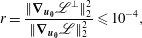 $$\begin{eqnarray}r=\frac{\Vert \unicode[STIX]{x1D735}_{\boldsymbol{u}_{\mathbf{0}}}\mathscr{L}^{\bot }\Vert _{2}^{2}}{\Vert \unicode[STIX]{x1D735}_{\boldsymbol{u}_{\mathbf{0}}}\mathscr{L}\Vert _{2}^{2}}\leqslant 10^{-4},\end{eqnarray}$$
reaching a sufficiently small threshold. A review of this method has been presented for instance in Schmid (Reference Schmid2007), as well as in Kerswell, Pringle & Willis (Reference Kerswell, Pringle and Willis2014) and Luchini & Bottaro (Reference Luchini and Bottaro2014) in the context of stability analysis with fully nonlinear dynamics.
2.3 Numerical model
All the results presented here have been produced with a modified version of the DAL method code wrapping the two-dimensional Navier–Stokes equations solver developed by Foures et al. (Reference Foures, Caulfield and Schmid2013) (see also Foures et al. (Reference Foures, Caulfield and Schmid2014)). The key (and dynamically significant) modification is that the scalar field has been made active, through the addition of the appropriate buoyancy terms. The code uses second-order finite differences on a staggered grid in the
 $y$
(spanwise) direction and spectral decomposition in the
 $x$
(streamwise) direction. Divergence-free conditions for the direct and adjoint velocity fields are ensured by means of Chorin’s projection algorithm (Chorin Reference Chorin1967, Reference Chorin1968). Time integration of diffusive terms is dealt with using a Crank–Nicolson scheme. A Runge–Kutta fourth-order scheme is used for the remaining terms except for the forcing term
 $(1-\unicode[STIX]{x1D6FC})\boldsymbol{u}$
in (2.12), which is treated implicitly. The simulations presented here have all been performed with
 $300$
Fourier modes in the
 $x$
direction and
 $200$
grid points in the
 $y$
direction, a resolution which convergence tests proved to be sufficient.
3 Numerical results
As noted in the Introduction, all the simulations presented here have been performed at Reynolds number
 $Re=500$
and Péclet number
 $Pe=500$
with the bulk Richardson number
 $0.01\leqslant Ri_{b}\leqslant 1.0$
. We also validated our simulations by reproducing the passive scalar mixing (
 $Ri_{b}=0$
) results of Foures et al. (Reference Foures, Caulfield and Schmid2014). In general, we have considered both time-averaged kinetic-energy maximisation (
 $\unicode[STIX]{x1D6FC}=0$
) and mix-norm minimisation (
 $\unicode[STIX]{x1D6FC}=1=\unicode[STIX]{x1D6FD}$
), with a target time
 $T=10$
. We have also considered variance minimisation (
 $\unicode[STIX]{x1D6FC}=1$
,
 $\unicode[STIX]{x1D6FD}=0$
), with the principal objective being to investigate whether mix-norm minimisation remains a good proxy for variance minimisation in density-stratified flows. Reaching numerical convergence is particularly challenging here because the problem, although two-dimensional, is fully nonlinear, and furthermore the adjoint evolution equations (2.12)–(2.13) are forced by the direct variables – all the more so for the
 $\unicode[STIX]{x1D6FC}=0$
case, where (2.12) is driven by an additional forcing term depending on the direct velocity field. This last feature requires very accurate evaluation of the direct fields for the sensitivities to be in turn correctly computed. It should also be emphasised that the DAL method only identifies local extrema. The first ‘guess’ initial condition consists of Gaussian noise in all the cases considered, thus hopefully ensuring that the initial perturbation is unlikely to have zero projection onto the true ‘optimal’ initial perturbation. In addition, the optimisation procedure was systematically initiated with different initial perturbations and always resulted in identifying the same (local) extremum. This observation is reassuring, although it cannot be ensured that this extremum actually is a global extremum due to the non-convexity of the optimisation problem.
3.1 Optimal initial perturbations in stratified fluids
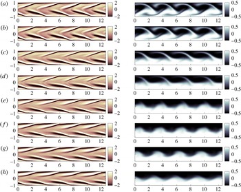
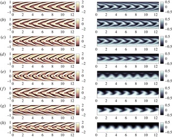
We plot the optimal initial perturbations associated with the time-averaged kinetic-energy maximisation problem and the mix-norm minimisation problem in the left-hand columns of figures 1 and 2 respectively, in terms of the (initial) vorticity field
 $\unicode[STIX]{x1D74E}_{\mathbf{0}}=\unicode[STIX]{x1D735}\times \boldsymbol{u}_{\mathbf{0}}$
for flows with eight different values of the bulk Richardson number
 $Ri_{b}$
. We plot the associated terminal scalar field
 $\unicode[STIX]{x1D70C}(x,y,T)$
in the right-hand columns of figures 1 and 2 respectively. Movies showing the time evolution of these fields for
 $Ri_{b}=\{0;0.05;0.1;0.2;0.5;1\}$
for the energy maximisation problem (movies 1 to 6) and
 $Ri_{b}=\{0;0.05;0.1;0.25;0.5;1\}$
for the mix-norm minimisation problem (movies 7 to 12) are also available as supplementary material at https://doi.org/10.1017/jfm.2018.565. Consistently with the observations of Foures et al. (Reference Foures, Caulfield and Schmid2014) for equivalent optimisation problems for a passive scalar with the same optimisation horizon
 $T=10$
, the dominant wavenumber selected for the optimal perturbation field is
 $m=4$
for the time-averaged kinetic-energy maximisation problem and
 $m=7$
for the mix-norm minimisation problem. (Foures et al. (Reference Foures, Caulfield and Schmid2014) found these optimal wavenumbers decrease as the time horizon
 $T$
increases for passive scalar flows.) For both problems when
 $Ri_{b}=0$
, the initial vorticity field consists of inclined, stretched vortices tilted into the shear of the base flow
 $U(y)$
, as defined in (2.1).
Initial perturbation vorticity
 $\unicode[STIX]{x1D735}\times \boldsymbol{u}_{\mathbf{0}}$
(on the left) and terminal deviation density field
 $\unicode[STIX]{x1D70C}$
at
 $T=10$
(on the right) for the time-averaged kinetic-energy maximisation problem for bulk Richardson number
 $Ri_{b}=$
(a–h): 0; 0.01; 0.05; 0.1; 0.2; 0.3; 0.5; 1. Movies 1–6 showing the time evolution of these fields for various
 $Ri_{b}$
are available as supplementary material.
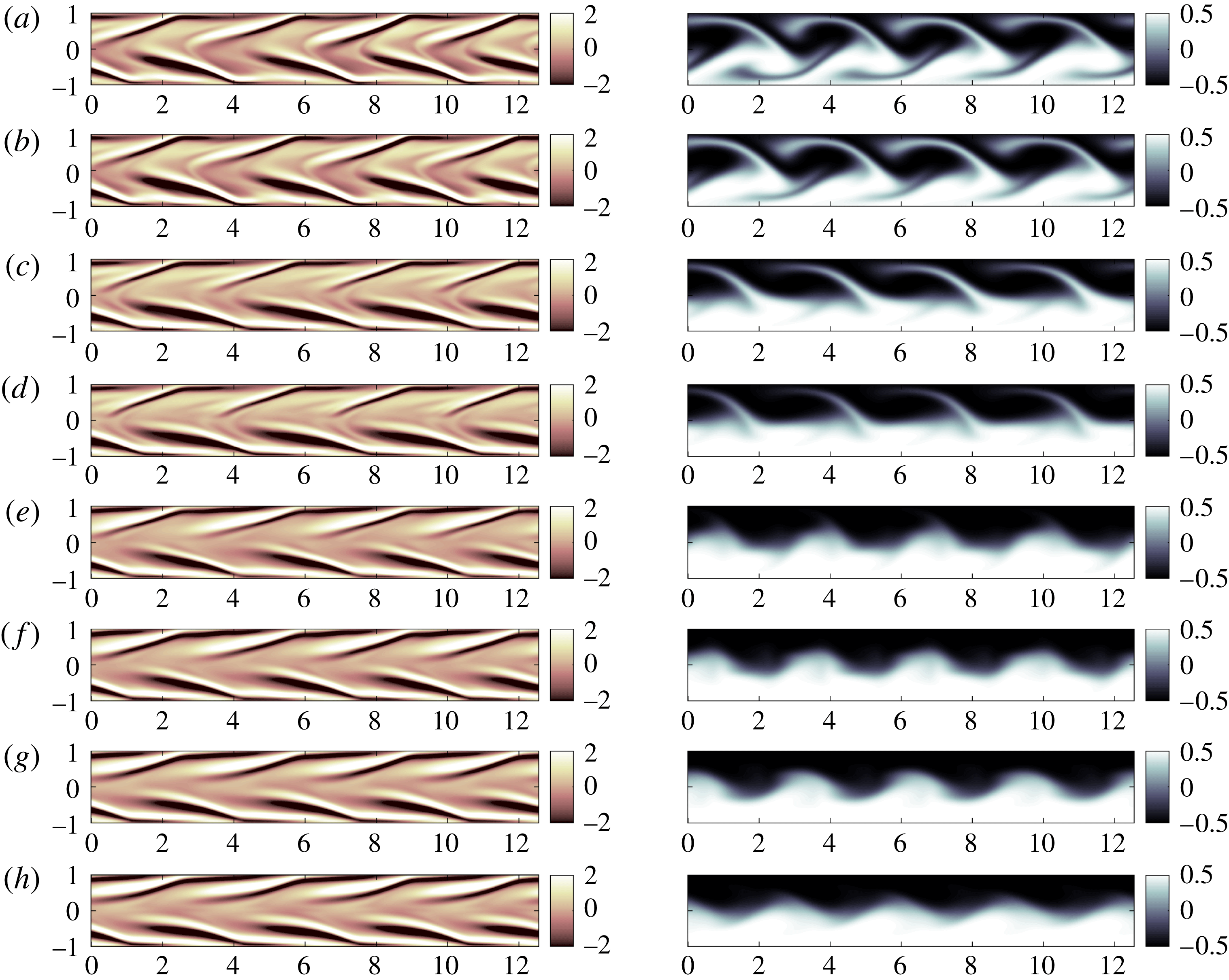
Initial perturbation vorticity
 $\unicode[STIX]{x1D735}\times \boldsymbol{u}_{\mathbf{0}}$
(left-hand column) and terminal deviation density field
 $\unicode[STIX]{x1D70C}$
at
 $T=10$
(right-hand column) for the mix-norm minimising problem for bulk Richardson number
 $Ri_{b}=$
(a–h): 0; 0.05; 0.1; 0.15; 0.2; 0.3; 0.5; 1. Movies 7–12 showing the time evolution of these fields for various
 $Ri_{b}$
are available as supplementary material.
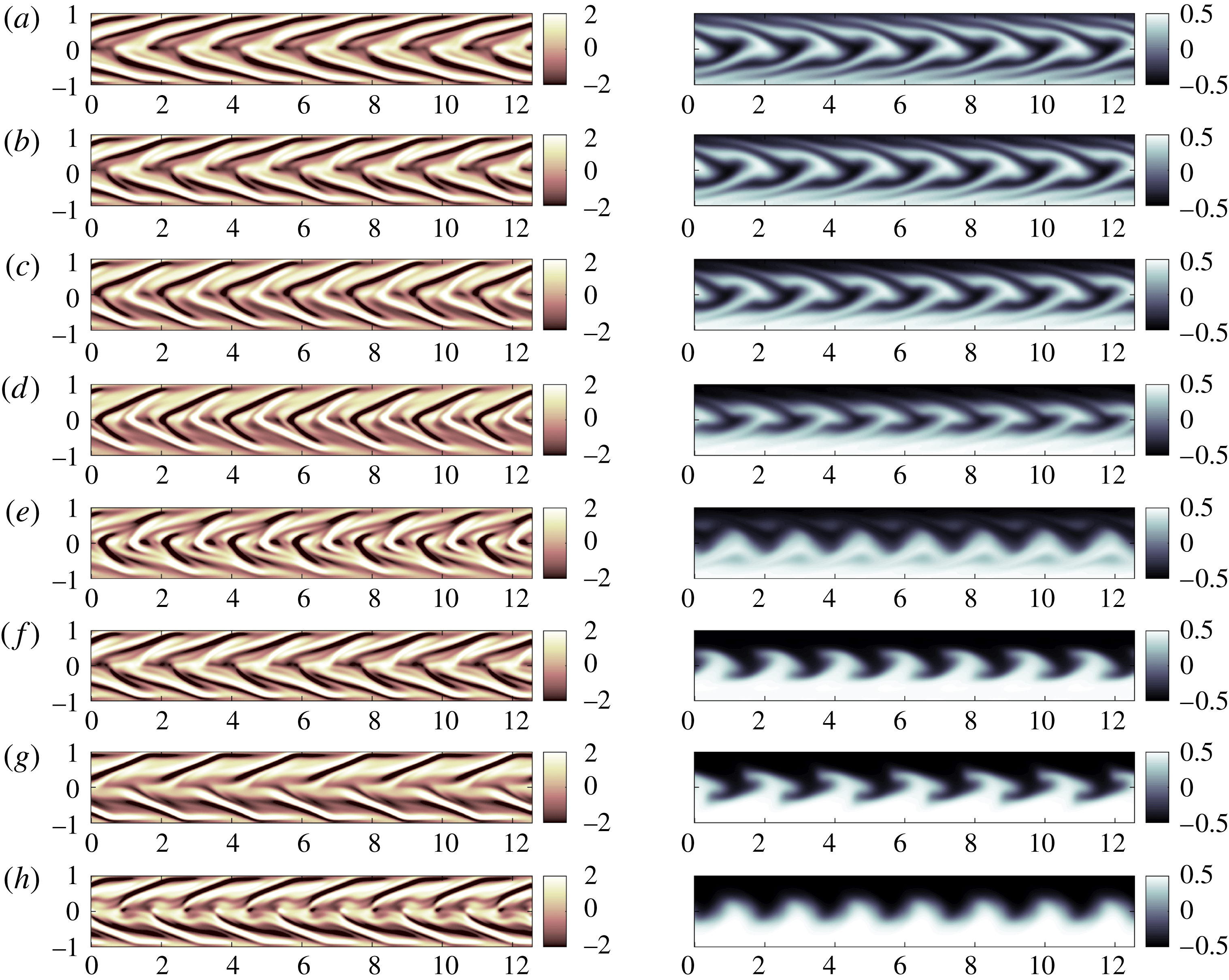
This flow configuration naturally favours transient energy growth due to the so-called Orr mechanism (Orr Reference Orr1907). The shear tilts the initially elongated vortices, transiently reducing their aspect ratio and their perimeters and hence increasing their energy by (close to) conservation of circulation, before again stretching them out into elongated vortices now inclined with the shear. Importantly, these optimal perturbation fields also take advantage of Taylor dispersion (Taylor Reference Taylor1953) to homogenise the density field. As part of the ‘transport’ phase as described in the Introduction and in Foures et al. (Reference Foures, Caulfield and Schmid2014), the perturbations transport dense fluid upwards and light fluid downwards towards the channel walls, where the locally strong base shear flow near the wall inevitably both sharpens the density gradients and further encourages filamentation and thus enhances diffusion.
However, the behaviour as stratification increases is markedly different for the two optimisation problems. As
 $Ri_{b}$
increases to non-trivial values between 0.05 and 1, the observed patterns (both for initial vorticity, and scalar distribution at terminal time) for the mix-norm minimisation problem do not change qualitatively. Increasing stratification does tend to inhibit transport of the stretched interface toward the walls, eventually resulting in the mixing being ineffective at sufficiently high
 $Ri_{b}$
. As can be seen in figure 2 showing the terminal density field at
 $Ri_{b}=1$
, the characteristic protruding, chevron-like structures which develop at lower
 $Ri_{b}$
have almost disappeared. Essentially, the interface is merely slightly displaced upwards and downwards, and so Taylor dispersion does not take place and the only irreversible modification is associated with relatively weak diffusion at the interface.
This transition to essentially ineffective mixing occurs in flows with much smaller
 $Ri_{b}$
for the time-averaged kinetic-energy maximisation problems. As plotted in figure 1, the two layers appear to remain completely distinct for a Richardson number as low as
 $Ri_{b}=0.2$
for these problems. Interestingly, stratification appears to affect the evolution of the density field for the time-averaged kinetic-energy maximisation problem in a more subtle way than it does for the mix-norm minimisation problem. Indeed, the complicated density structure observed for flows with low
 $Ri_{b}$
results from strong filamentation and subsequent roll up of the already folded interface, which starts to develop as soon as the peak in kinetic energy is reached. In the absence of buoyancy forces (
 $Ri_{b}=0$
) the resulting structure essentially exhibits up–down symmetry, a symmetry which appears to be broken for the flows with relatively weak stratification (i.e. with
 $Ri_{b}=0.01-0.1$
). Furthermore, this apparent symmetry breaking is accompanied by a progressive disappearance of the filaments as
 $Ri_{b}$
increases towards
 $Ri_{b}=0.2$
, where they actually vanish. However, looking at the time evolution of the density field (as in the accompanying supplementary material movies) reveals that rolling up of the density distribution occurs both in the upper half-plane and the lower half-plane, alternating in time. This particular process of alternating roll up is a dynamical process which is switched off for flows with
 $Ri_{b}\gtrsim 0.2$
.
Finally, it is important to appreciate that the apparently anomalous behaviour of the mix-norm minimising problem for
 $Ri_{b}=0.2$
(in point of fact very similar to the behaviour of a flow with
 $Ri_{b}=0.25$
, which for reasons of space is not displayed in figure 2), is best understood as a somewhat misleading snapshot in its time evolution. The transition in behaviour as
 $Ri_{b}$
increases from
 $Ri_{b}=0.15$
to
 $Ri_{b}=0.3$
occurs as the largest parts of the periodic density ‘chevrons’ fall back toward the centre of the channel under the increasing effect of gravity earlier and earlier in the flow evolution, as is apparent from the movies of the flow evolution available as supplementary materials. Indeed their filamented remnants are still visible near the boundaries in the flow for
 $Ri_{b}=0.2$
, and the snapshot shown in the figure is just at the ‘wrong’ stage in the flow evolution to show the chevron structures clearly. As the stratification gets stronger, with
 $Ri_{b}\gtrsim 0.3$
, buoyancy forces suppress the chevron structure developing so that the filaments cease to interact significantly with the heightened shear near the channel walls.
3.2 Comparing the objective functionals
Such qualitative comparisons of the terminal density fields for various
 $Ri_{b}$
are highly suggestive that the time-averaged kinetic-energy maximising initial perturbation is less effective than the mix-norm minimising initial perturbation at stratified mixing at
 $Re=Pe=500$
, at least for
 $Ri_{b}>0.2$
. This suggestion can be confirmed and extended to all Richardson numbers by quantitatively assessing the well-mixedness of the flow at long times.
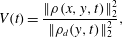
Even though the mix-norm is used in the definition of the cost functional in our optimisation problems (for the computational reasons given above) the variance is still the natural physical measure which should be used as a diagnostic for the well-mixedness or homogenisation of the initially stratified fluid. One way to consider an aspect of the time-dependent ‘quality’ of mixing by the various flows is to compute an instantaneous normalised variance (following Foures et al.
Reference Foures, Caulfield and Schmid2014)
 $V(t)$
, defined as the ratio of the variance of the density field at instant
 $t$
to the variance of the initial base density field at the same instant under the action of pure diffusion:
 $$\begin{eqnarray}V(t)=\frac{\Vert \unicode[STIX]{x1D70C}(x,y,t)\Vert _{2}^{2}}{\Vert \unicode[STIX]{x1D70C}_{d}(y,t)\Vert _{2}^{2}},\end{eqnarray}$$
where
 $\unicode[STIX]{x1D70C}_{d}(y,t)$
is the one-dimensional solution of the purely diffusion version of the density deviation evolution equation (2.5) (assuming
 $\boldsymbol{u}=\boldsymbol{U}=0$
) with initial condition
 $\unicode[STIX]{x1D70C}_{i}(\boldsymbol{x})$
as given in (2.3). Small values of
 $V(t)$
therefore denote well-mixedness of the flow induced by fluid motions.
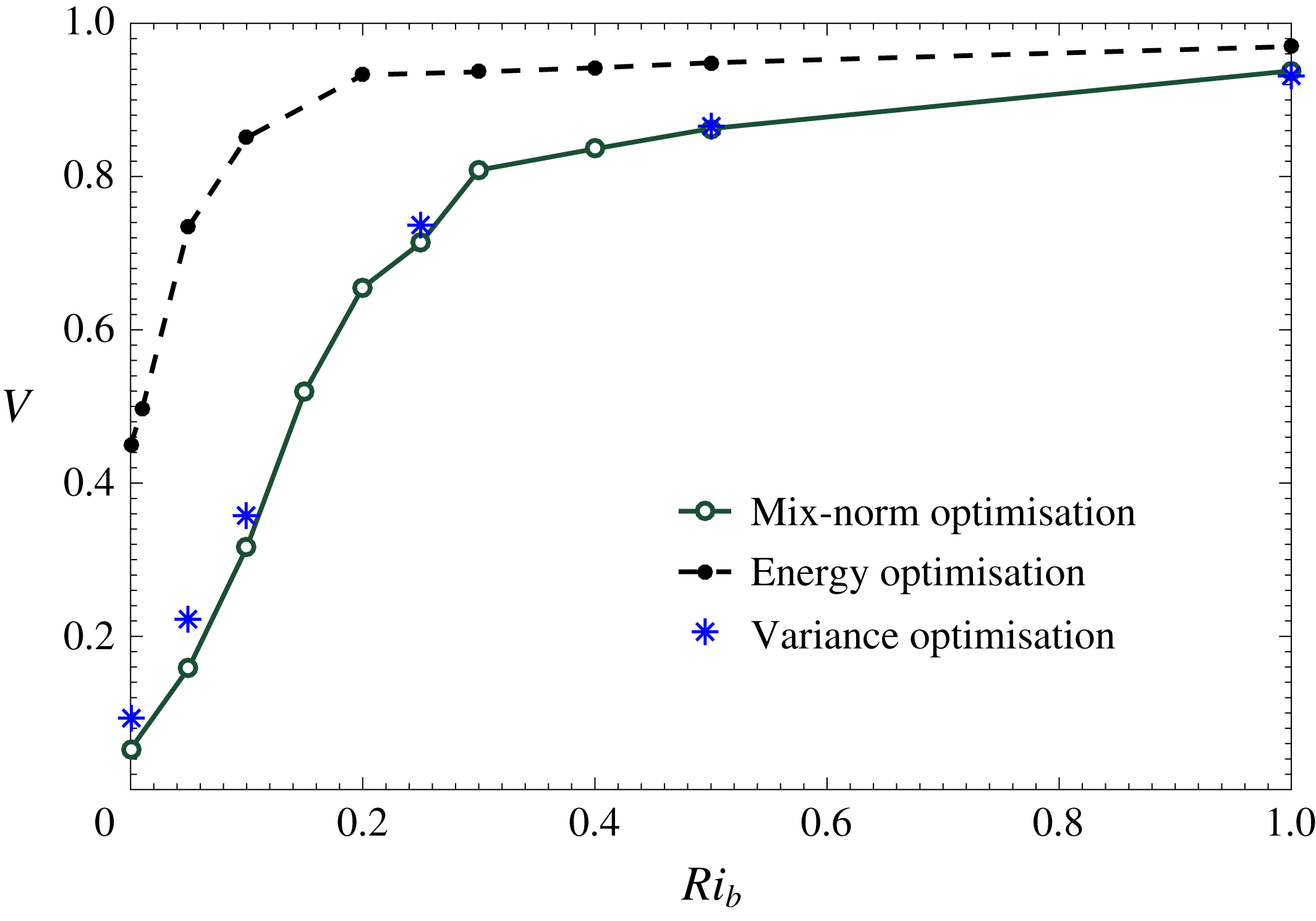
Variation with
 $Ri_{b}$
of the scaled variance
 $V$
(as defined in (3.1)) at time
 $t=30$
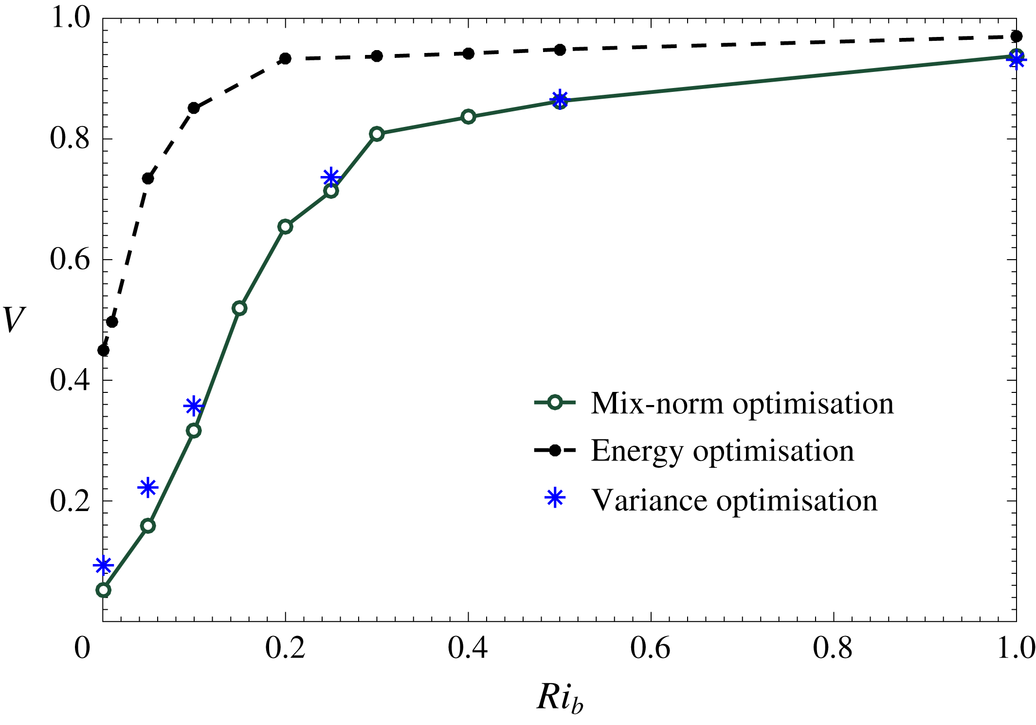
for: time-averaged kinetic-energy maximisation problem flows (plotted with a dashed line) and mix-norm minimisation problem flows (solid line), all for the intermediate time horizon
 $T=10$
. For comparison, stars mark the values of the scaled variance at
 $t=30$
for variance minimisation problem flows, calculated for the same intermediate time horizon of
 $T=10$
.
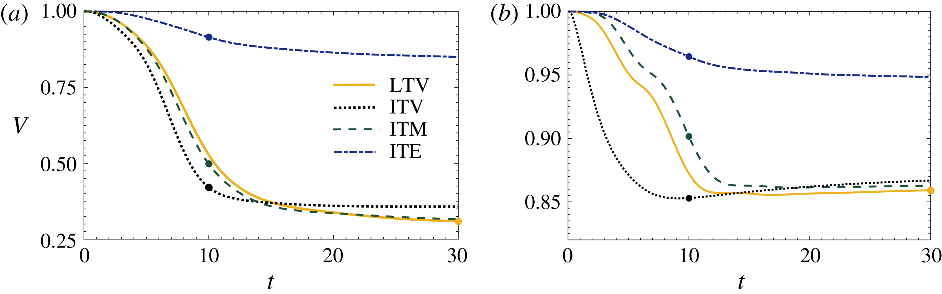
For flows with: (a)
 $Ri_{b}=0.1$
; (b)
 $Ri_{b}=0.5$
; time evolution of the scaled variance
 $V$
(as defined in (3.1)) for different optimisation problem flows where two target times
 $T$
have been considered for comparison: long-time (
 $T=30$
) variance minimisation flow (LTV; plotted with a solid line), intermediate-time (
 $T=10$
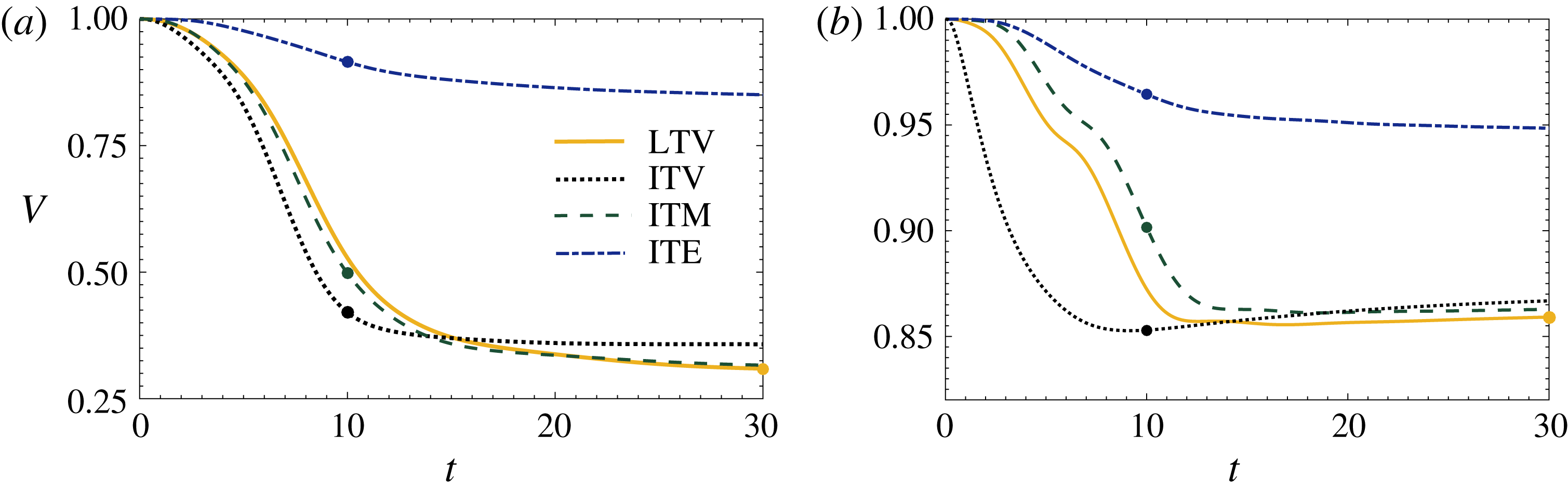
) variance minimisation flow (ITV; dotted line), intermediate-time mix-norm minimisation flow (ITM; dashed line) and intermediate-time energy maximisation flow (ITE; dotted/dashed line). For each case, the target time for optimisation is highlighted with a colour-filled circle.
In figure 3, we plot the normalised variance
 $V(30)$
achieved at time
 $t=30$
for three different optimisation problem flows, all of which are calculated over what we refer to as the ‘intermediate’ time horizon
 $[0,10]$
. The results for the flows that maximise the time-averaged perturbation kinetic energy are plotted with a dashed line, the results for the flows that minimise the mix-norm are plotted with a solid line, while the results for the flows that minimise the variance over the same intermediate time horizon
 $[0,10]$
are given for reference and plotted with star symbols. For this measure, it is clear that the perturbations which minimise the mix-norm are significantly more effective than the perturbations which maximise the time-averaged perturbation kinetic energy at identifying flows which enhance the reduction in the scalar variance through advection, whatever the degree of stratification. Furthermore, although (stable) stratification always tends to inhibit homogenisation significantly (in that
 $V(t)$
increases with
 $Ri_{b}$
), the transition towards poor homogenisation (i.e. close to purely diffusive homogenisation, with the scaled variance
 $V(t)\simeq 1$
) occurs at much higher Richardson numbers for the flows arising from the mix-norm minimisation problem.
In the flow arising from the time-averaged kinetic-energy maximisation problem,
 $V(t)$
essentially reaches a plateau as soon as the filamented structures vanish (with
 $V(30)\sim 0.9$
at
 $Ri_{b}=0.2$
), implying that flow-induced mixing is largely ineffective for stronger stratifications for such perturbations. These observations extend the results of Foures et al. (Reference Foures, Caulfield and Schmid2014), who, considering a passive scalar, demonstrated that perturbations which maximise the time-averaged perturbation kinetic energy are significantly suboptimal in minimising the scalar variance over finite-time horizons. We find that this statement holds true for an active scalar, and is even made stronger in the presence of a statically stable stratification.
Furthermore, the results presented in figures 3 and 4 provide further evidence that the mix-norm is a robust, useful and computationally attractive measure to use in mixing optimisation problems, even when there are buoyancy forces involved. Indeed, by comparison of the curves for the variance minimisation flows and the mix-norm minimisation flows, the variance for the mix-norm minimising flows is typically slightly smaller at the late time
 $t=30$
, except for the extreme flow with
 $Ri_{b}=1$
, where the flow is ineffective at mixing, and the difference is very small. This does not demonstrate a break down in the optimisation procedure of course, since our calculations are minimising the measure of interest over intermediate times (i.e.
 $T=10$
), while the figure plots the subsequent behaviour of the flow at late times (i.e.
 $t=30$
).
Entirely consistently with the results of Foures et al. (Reference Foures, Caulfield and Schmid2014), initial optimal perturbations which lead to minimisation of variance over relatively short times are non-trivially different from optimal perturbations which lead to variance minimisation at long times, typically because such shorter time optimal perturbations are relatively fine scale, and so do not lead to thorough mixing across the channel. On the other hand, the mix-norm minimisation optimal perturbations over intermediate times are close approximations to the variance minimising optimal perturbations over long times, although their computational calculation is much shorter for two reasons. First, the loops at the heart of the DAL method are obviously shorter when optimising over shorter target times. Second, the number of iterations around such loops are also typically and substantially smaller, as values of the mix-norm decrease more rapidly in time than the values of the variance. This second phenomenon can be appreciated through consideration of the (non-dimensional) forms of the two evolution equations for these measures (1.2) and (1.4). For the variance, the term on the right-hand side of (1.2) is scaled with
 $1/Pe$
, and so in general inevitably decays slowly for large
 $Pe$
, while the first term on the right-hand side of (1.4) typically ensures that the mix-norm decays more rapidly.
Significantly, we find that this usefulness of mix-norm minimisation over intermediate times as a computationally efficient and robust proxy for variance minimisation over longer times also occurs for flows with all values of the bulk Richardson number which we have considered. This is a major result of this study, as it demonstrates that use of the mix-norm remains appropriate for flows where the problem of interest is the optimisation of the (irreversible) mixing of a active scalar. To illustrate this observation further, in figures 4(a) and 4(b) for flows with
 $Ri_{b}=0.1$
and
 $Ri_{b}=0.5$
respectively, we plot the time evolutions of the scaled variance for four different optimisation problems. In each case, the key comparison is with the evolution of the variance for the variance minimisation flow over the relatively long time interval
 $T=30$
, labelled ‘LTV’, and plotted with a solid line. It is clear that minimisation of the mix-norm with the ‘intermediate’ target time
 $T=10$
(labelled ‘ITM’, and plotted with a dashed line) leads to significantly more mixing at time
 $t=30$
than the variance minimisation flow over the same intermediate target time
 $T=10$
(labelled ‘ITV’, and plotted with a dotted line), and even yields similar variance at time
 $t=30$
to the LTV flow.
Note at the intermediate target time
 $T=10$
, the variance of the ITV flow is indeed, in both cases, smaller than the variance of the ITM flow, as expected. It is perhaps counter-intuitive that there is a slight increase in the scaled variance evolution for ITM, ITV and LTV flows at
 $Ri_{b}=0.5$
. It is important to appreciate that these quantities are scaled by the (time-dependent) variance of the density distribution experiencing pure diffusion (i.e. with no macroscopic velocity
 $\boldsymbol{u}=\boldsymbol{U}=\mathbf{0}$
). At early times, the various optimal solutions develop very strong gradients, rapidly suppressed by diffusion, and so the variance drops very quickly. At later times therefore, the rate of decrease of variance of a close-to-homogeneous distribution can be extremely slow, indeed slower than the rate associated with the purely diffusing solution, and so the scaled variance can increase (slightly).
The apparent particular robustness of mix-norm-based optimisation is due to the mix-norm mathematical definition, which (as mentioned in the Introduction) favours filamentation of the scalar field. Indeed, variance-based optimisation leads to the suppression of all heterogeneities by the time horizon, whereas mix-norm-based optimisation favours creation of small scales and sharp, filamented structures in the scalar field. These structures are then left for diffusion to smooth them out even after the target time, leading to further decrease of the scalar variance. Optimisation of the variance over too short a target time does not ensure thorough mixing throughout the entire width of the channel. Therefore, even for stratified flows, we believe it is appropriate to analyse in further detail the properties of the results from the mix-norm minimisation ITM flows.
4 Energy reservoir exchange
4.1 Available and background potential energy
A major distinguishing characteristic of mixing of active scalars in stratified fluids is that there is an energetic cost to the mixing in that the potential energy of the system is ultimately increased irreversibly when mixing occurs in an initially statically stable fluid. This fundamental characteristic has profound effects on the dynamics of stratified mixing, and continues to be a topic of much ongoing research and controversy. Taking the appropriate volume-averaging scalar product of the Navier–Stokes equations (2.4) with the velocity field
 $\boldsymbol{u}$
yields, after integration by parts and application of various boundary conditions, we obtain the evolution equation for the perturbation kinetic energy density
 $K=\Vert \boldsymbol{u}\Vert _{2}^{2}/2$
:
 $$\begin{eqnarray}\frac{\text{d}K}{\text{d}t}=-\frac{Ri_{b}}{V_{\unicode[STIX]{x1D6FA}}}\int _{\unicode[STIX]{x1D6FA}}\unicode[STIX]{x1D70C}v\,\text{d}\unicode[STIX]{x1D6FA}-\frac{1}{V_{\unicode[STIX]{x1D6FA}}}\int _{\unicode[STIX]{x1D6FA}}uv\frac{\unicode[STIX]{x2202}U}{\unicode[STIX]{x2202}y}\,\text{d}\unicode[STIX]{x1D6FA}-\frac{1}{ReV_{\unicode[STIX]{x1D6FA}}}\int _{\unicode[STIX]{x1D6FA}}\unicode[STIX]{x1D735}\boldsymbol{u}^{\text{T}}\boldsymbol{ : }\unicode[STIX]{x1D735}\boldsymbol{u}\,\text{d}\unicode[STIX]{x1D6FA}.\end{eqnarray}$$
The various contributions on the right-hand side are readily identified with various key physical processes, and we rewrite (4.1) in the more compact form
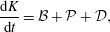 $$\begin{eqnarray}\frac{\text{d}K}{\text{d}t}={\mathcal{B}}+{\mathcal{P}}+{\mathcal{D}},\end{eqnarray}$$
where
 ${\mathcal{B}}$
denotes the buoyancy flux exchange between the kinetic energy and the potential energy reservoirs,
 ${\mathcal{P}}$
denotes the Reynolds stress-mediated energy transfer rate from the pressure-driven base flow
 $\boldsymbol{U}$
to the perturbation field
 $\boldsymbol{u}$
, and
 ${\mathcal{D}}$
denotes the negative definite viscous dissipation rate of conversion of perturbation kinetic energy into internal energy. Once again, it is important to remember that there is no assumption that the perturbation velocity here is small compared to the base flow, or indeed that it has zero streamwise mean instantaneously.
Similarly, the evolution equation for the potential energy density
 $P=Ri_{b}/V_{\!\unicode[STIX]{x1D6FA}}\!\int _{\unicode[STIX]{x1D6FA}}(\unicode[STIX]{x1D70C}y)\text{d}\unicode[STIX]{x1D6FA}$
(associated with the dimensionless density deviation
 $\unicode[STIX]{x1D70C}$
) can be derived from (2.5):
 $$\begin{eqnarray}\frac{\text{d}P}{\text{d}t}=\frac{Ri_{b}}{V_{\unicode[STIX]{x1D6FA}}}\int _{\unicode[STIX]{x1D6FA}}\unicode[STIX]{x1D70C}v\,\text{d}\unicode[STIX]{x1D6FA}+\frac{Ri_{b}}{PeV_{\unicode[STIX]{x1D6FA}}}\int _{\unicode[STIX]{x1D6FA}}(\unicode[STIX]{x1D6FB}^{2}\unicode[STIX]{x1D70C})y\,\text{d}\unicode[STIX]{x1D6FA}=-{\mathcal{B}}+{\mathcal{D}}_{\unicode[STIX]{x1D70C}},\end{eqnarray}$$
where
 ${\mathcal{D}}_{\unicode[STIX]{x1D70C}}$
denotes the conversion rate of internal energy into potential energy by diffusion of a statically stable density distribution. Exchanges between the kinetic energy and potential energy reservoirs are possible through the buoyancy flux contribution in (4.1)–(4.3). These exchanges typically have both reversible and irreversible components. Lorenz (Reference Lorenz1955) first introduced the concept of available potential energy in order to refer to the fraction of potential energy which can be converted back into kinetic energy by buoyancy flux. In the absence of any buoyant motion, i.e. if the stratification is statically stable everywhere and the density gradient is parallel to the gravity field, this available potential energy is therefore zero. The remaining fraction is conventionally labelled the background potential energy (see for example Winters et al. (Reference Winters, Lombard, Riley and Dasaro1995), and Peltier & Caulfield (Reference Peltier and Caulfield2003) for a review) and is notionally defined as the minimum potential energy obtainable by adiabatic spatial redistribution of the density field (which forms the so-called background state).
This partitioning of total potential energy into available and background potential energy is a convenient way of distinguishing between two different situations. In the first, completely reversible situation, the displaced fluid particles fall back to their neutrally buoyant position and the potential energy stored in their initial displacement is entirely converted back into kinetic energy. This may be said to correspond to ‘stirring’ of the scalar field by the velocity field. In the second situation, fluid motion modifies the density field at sufficiently small scales for diffusive fluxes to be enhanced, such that the background state is modified, increasing the background potential energy and irreversible ‘mixing’ occurs. In order to account for the enhancement of diffusive fluxes by stirring (compared to the purely conductive case), we can thus define, following Caulfield & Peltier (Reference Caulfield and Peltier2000) and Peltier & Caulfield (Reference Peltier and Caulfield2003) the irreversible (advective) mixing rate
 ${\mathcal{M}}$
, which acts as a sink in the evolution equation for the available potential energy
 $P_{A}$
and as a source for the background potential energy
 $P_{B}$
(remembering that the total potential energy density
 $P=P_{A}+P_{B}$
by construction):
 $$\begin{eqnarray}\frac{\text{d}P_{A}}{\text{d}t}=-\,{\mathcal{B}}\,-\,{\mathcal{M}},\quad \frac{\text{d}P_{B}}{\text{d}t}={\mathcal{M}}+{\mathcal{D}}_{\unicode[STIX]{x1D70C}}.\end{eqnarray}$$
As in Caulfield & Peltier (Reference Caulfield and Peltier2000), the instantaneous background potential energy
 $P_{B}$
is determined at any time by spatially redistributing the density field using a sorting algorithm. It is possible to calculate
 ${\mathcal{D}}_{\unicode[STIX]{x1D70C}}$
directly from (4.3), and then
 ${\mathcal{M}}$
can be determined from (4.4). To understand the actual irreversible mixing processes which occur in the flows we are considering, it is therefore illuminating to analyse the evolution of the energy stored in the different reservoirs as the flows determined by the two different optimisation problems evolve. Note that, differently from Winters et al. (Reference Winters, Lombard, Riley and Dasaro1995), we distinguish between the irreversible mixing inherently due to motion, occurring at a rate
 ${\mathcal{M}}$
, and the increase in
 $P_{B}$
that would occur in the absence of macroscopic motion, occurring at a rate
 ${\mathcal{D}}_{\unicode[STIX]{x1D70C}}$
. It is also important to remember that since we are considering an incompressible Boussinesq fluid with a linear equation of state, the true thermodynamics of stratified mixing and the exchanges between the different reservoirs have been significantly simplified. These important aspects have been reviewed in detail in Tailleux (Reference Tailleux2013).
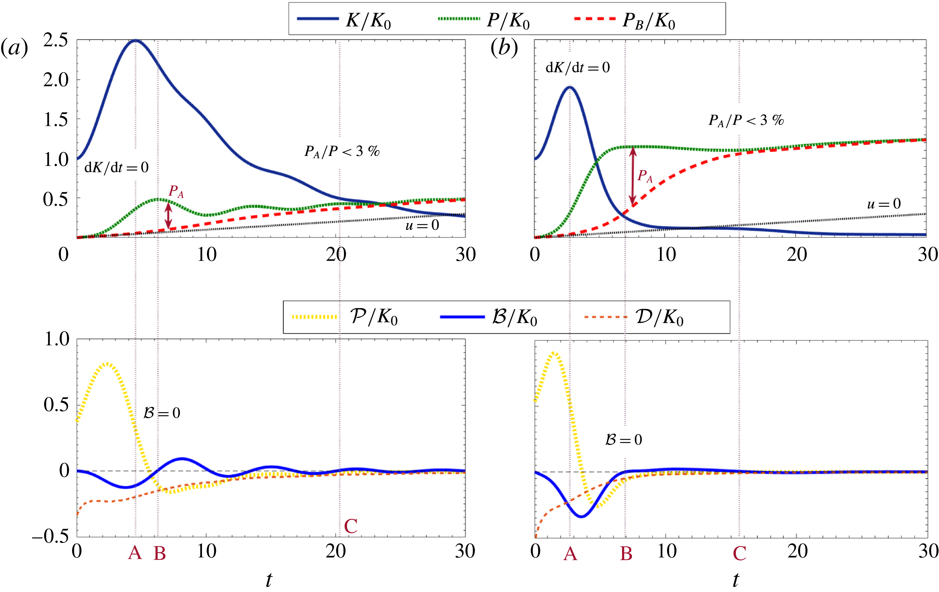
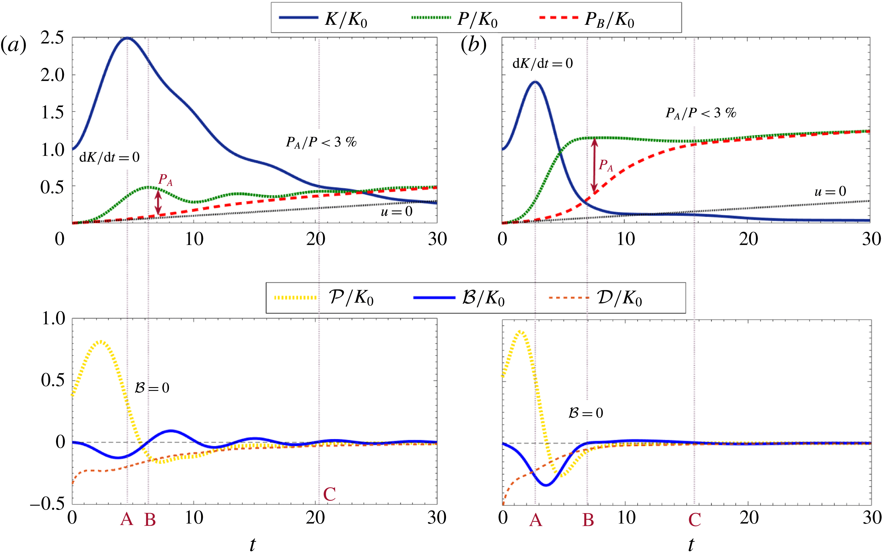
Variation with time of: (upper panels) scaled kinetic energy density
 $K/K_{0}$
(plotted with a solid line), scaled total potential energy
 $P/K_{0}$
(dotted line), scaled background potential energy density
 $P_{B}/K_{0}$
(dashed line) and scaled potential energy of the purely diffusing solution
 $\unicode[STIX]{x1D70C}_{d}(y,t)$
(thinner dotted line); (lower panels) the scaled buoyancy flux
 ${\mathcal{B}}/K_{0}$
(plotted with a solid line), viscous dissipation rate
 ${\mathcal{D}}/K_{0}$
(dashed line) and energy transfer rate
 ${\mathcal{P}}/K_{0}$
(dotted line), as defined in (4.1)–(4.2). The data come from simulations of flows with
 $Ri_{b}=0.1$
associated with initial perturbations which: (a) maximise the time-averaged perturbation kinetic energy; (b) minimise the mix-norm. In the upper panels, the available potential energy
 $P_{A}$
corresponds to the difference between the (thicker) dotted lines and the dashed lines. The following dimensionless times, which correspond to the specific events indicated on the plots and discussed in the text, are given for reference: ‘A’
 $=4.5$
, ‘B’
 $=6.2$
, ‘C’
 $=20.3$
(time-averaged kinetic-energy maximising case); ‘A’
 $=2.7$
, ‘B’
 $=6.9$
, ‘C’
 $=15.7$
(mix-norm minimising case).
4.2 Time evolution of energy reservoirs
In what follows, the two types of initial perturbations, determined by considering the ‘intermediate’ time horizon
 $T=10$
for the time-averaged kinetic-energy maximisation problem and the mix-norm minimisation problem, are added to the pressure-driven base flow
 $U(y)$
, defined in (2.1), and initial density deviation
 $\unicode[STIX]{x1D70C}_{i}(x)$
, defined in (2.3). These initial conditions are then used to integrate the flow forwards to the ‘long’ time
 $t=30$
. We calculate the kinetic-energy density, the total potential energy density and the background potential energy density at each time step. We plot the time evolution of these energies in figure 5 for the two different flows with
 $Ri_{b}=0.1$
, along with the contributions of the different terms as defined in (4.2). The evolution of the potential energy (equivalent in this specific case to the background potential energy) of the purely diffusive solution
 $\unicode[STIX]{x1D70C}_{d}(y,t)$
(with
 $\boldsymbol{u}=\boldsymbol{U}=\mathbf{0}$
) used to scale the normalised variance
 $V(t)$
, has been superimposed for reference (plotted with thinner dotted lines in the upper panels of figure 5).
As can observed from the time evolution of buoyancy flux in the lower panels of figure 5, all the dynamically important buoyancy-driven motions have clearly finished significantly before the chosen final time
 $t=30$
for the flow with
 $Ri_{b}=0.1$
. It is important to remember that the key (dimensional) time scale of buoyancy-driven motions is proportional to
 $\sqrt{\bar{\unicode[STIX]{x1D70C}}^{\ast }/(g^{\ast }\unicode[STIX]{x1D70C}_{0}^{\ast })}$
, and so, in the chosen non-dimensionalisation scheme, the characteristic buoyancy time scale is inversely proportional to the square root of the bulk Richardson number
 $Ri_{b}$
. Therefore, we believe that using
 $t=30$
as the final time for our various analyses is appropriate to capture important buoyancy-driven processes for the various stratified flows considered here, particularly for the flows with
 $Ri_{b}\geqslant 0.1$
where buoyancy becomes increasingly significant.
The time evolution develops through four phases, divided on the figures by vertical dot-dashed lines. There is a clear relationship to the three stages of ‘transport’, ‘dispersion’ and ‘relaxation’ discussed in the context of passive scalar mixing by Foures et al. (Reference Foures, Caulfield and Schmid2014), although the possibility of exchange between the kinetic energy and potential energy reservoirs makes the behaviours of these stratified flows inevitably more complicated. During the first phase (up to the instant labelled ‘A’ on figure 5), the kinetic energy
 $K$
experiences transient growth as energy is transferred from the base flow to the perturbation at the ‘production’ rate
 ${\mathcal{P}}$
. This stage has a longer duration in the flow associated with the energy maximisation problem (a) than in the flow associated with mix-norm minimisation (b), and results in a significantly higher kinetic energy at its peak. This is unsurprising, since perturbation energy is of course being maximised in one flow and not in the other. This phase corresponds to an initial part of the ‘transport’ phase of mixing, where much of this growth of perturbation kinetic energy can be associated with extraction of kinetic energy from the base flow via the Orr mechanism.
In the second phase, (between the instants marked ‘A’ and ‘B’) the kinetic energy decreases and
 ${\mathcal{B}}<0$
. Therefore, the energy transfer rate from the base flow is no longer sufficient to counteract the combined effects of the viscous dissipation rate
 ${\mathcal{D}}$
converting kinetic energy into internal energy and the buoyancy flux
 ${\mathcal{B}}$
converting kinetic energy into potential energy. During this phase, since
 ${\mathcal{B}}<0$
, the potential energy increases. The energetic perturbation is lifting up dense fluid and pushing down light fluid to create the vertical ‘stripe’, rapidly distorted to ‘chevron’ structure conducive to subsequent mixing, and characteristic of a later part of the initial ‘transport’ stage.
Both
 $P_{A}$
and
 $P_{B}$
increase for both flows, but there is substantial qualitative difference between the two flows. In the flow associated with (kinetic) energy maximisation,
 $P_{B}$
increases only slightly faster than the purely diffusive solution (plotted with the thinner dotted line), as
 $M$
is very small in magnitude, and the perturbation kinetic energy does not actually decrease substantially. Even more (ultimately) significantly, the total potential energy
 $P$
(plotted with the thicker dotted line) grows to a much smaller maximum value than in the flow associated with mix-norm minimisation. In the mix-norm minimisation flow,
 $P_{B}$
(plotted with a dashed line) also grows much more strongly during this stage, (associated with a much larger value of
 $M$
, the advective irreversible mixing rate). For this flow, the kinetic energy has decreased much more significantly, and the flow arrangement appears to be consistent with the perturbation kinetic energy ‘efficiently’ being exchanged into potential energy.
The second phase finishes (at ‘B’) when the total potential energy density
 $P$
reaches a (local) maximum, and equivalently when the buoyancy flux
 ${\mathcal{B}}=0$
. The third (and longest) phase (between the times marked ‘B’ and ‘C’) is the phase during which the majority of the irreversible mixing occurs, with
 $P_{B}$
increasing and
 $P_{A}$
decreasing, until the total potential energy and the background potential energy are within
 $3\%$
of each other. This phase naturally corresponds to the second ‘dispersion’ phase of (significant) mixing, while the fourth phase (when
 $P_{B}\lesssim P$
) for times after ‘C’ clearly corresponds to the final diffusion-dominated ‘relaxation’ stage discussed by Foures et al. (Reference Foures, Caulfield and Schmid2014).
As can be seen in figure 5(a), in the flow associated with the time-averaged kinetic-energy maximisation problem, the background potential energy increases monotonically with almost equal contributions from the (notional) diffusive conversion of internal energy and the decrease of available potential energy. Furthermore, for this flow, the total potential energy varies non-monotonically, with the buoyancy flux mediating a quasi-periodic oscillatory exchange between the kinetic energy and the potential energy reservoirs.
The behaviour of the flow associated with the mix-norm minimisation problem during this significant mixing phase (or equivalently the ‘dispersion’ stage) is qualitatively different, with a much larger increase in the background potential energy. Furthermore, there is a very marked damping of subsequent buoyancy flux oscillations. Essentially, virtually all the energy stored as available potential energy by the development of the perturbation during the first two phases (i.e. during the ‘transport’ stage either due to kinetic energy increase or potential energy increase) of the flow evolution is converted into background potential energy, and thus is associated with irreversible mixing during this phase.
Therefore, there are two key characteristics of this flow which appear to be conducive to mixing. First, a relatively large amount of energy is converted into potential energy. Second, virtually all of this energy is ‘captured’ as background potential energy through irreversible mixing in a single pass, without oscillatory, and hence at least partially reversible, exchange with the kinetic-energy reservoir. Two natural questions then arise. First, can these two characteristics be identified with particular physical processes identifiable in the flow evolution? Second, do these characteristics lead to significant differences in the efficiency of the mixing in an energetic sense (as defined in 4.4), analogous to that defined in the context of transient shear instability-driven stratified mixing considered by Winters et al. (Reference Winters, Lombard, Riley and Dasaro1995) and Caulfield & Peltier (Reference Caulfield and Peltier2000)?
4.3 Flow evolution and physical interpretation
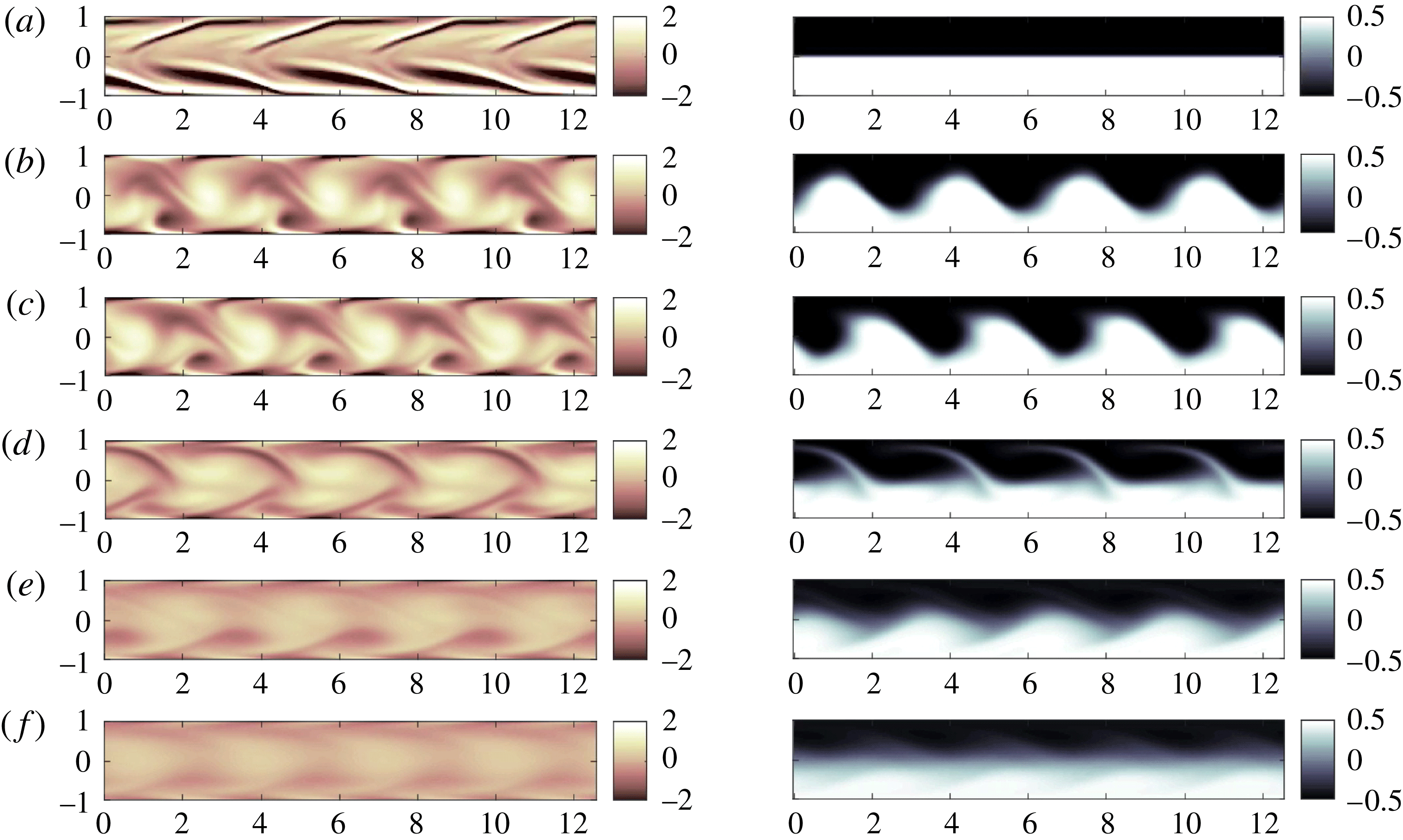
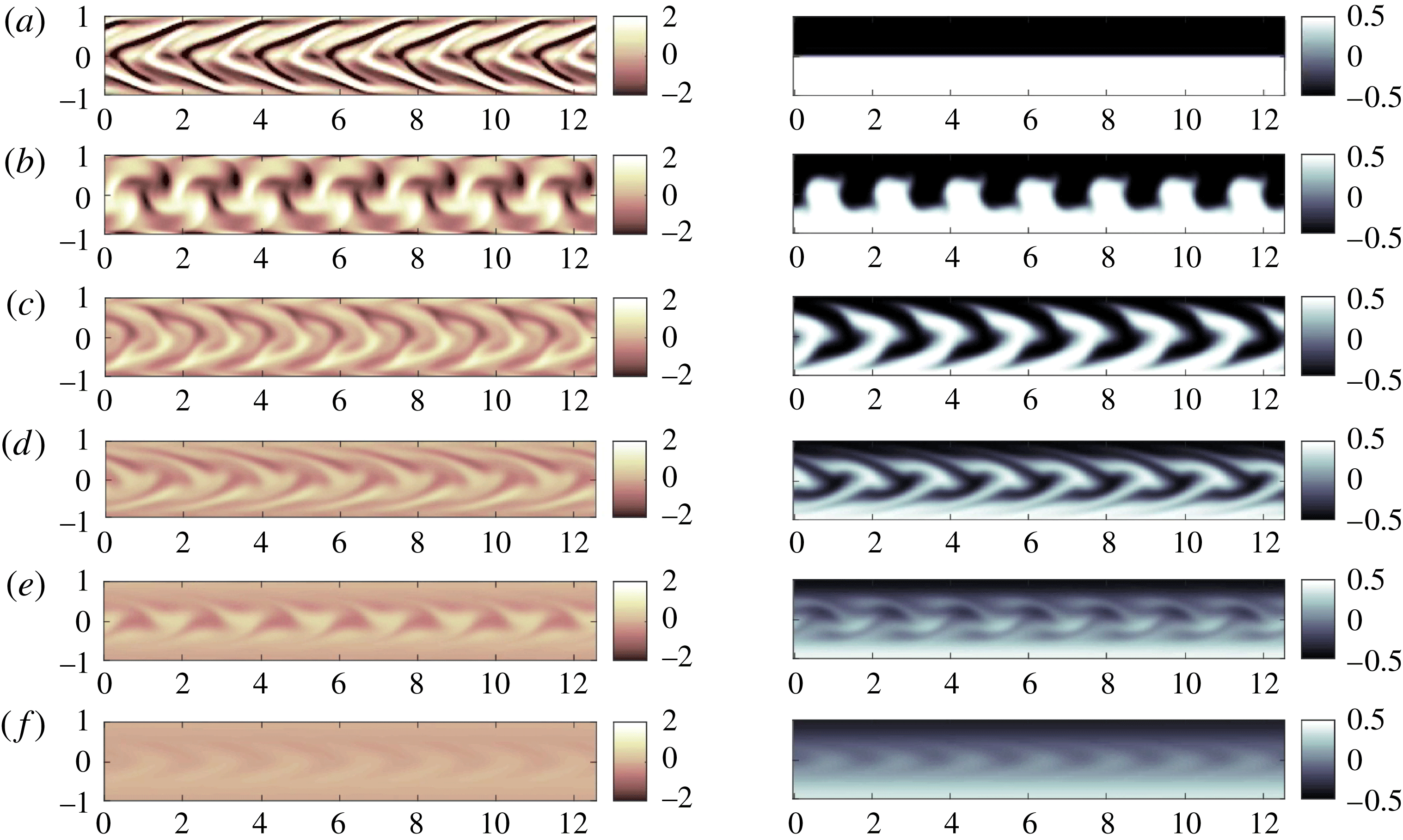
The four different phases in the evolution of the energy reservoirs can be identified with a succession of flow structures plotted in figures 6 and 7, where the perturbation vorticity field and density deviation field are shown. In both flows, the first peak in total potential energy (marked as ‘B’) is achieved when the initially prescribed vorticity field has distorted the interface maximally, and brought light fluid to a minimal height and dense fluid to a maximum height, completing the initial transport stage. As expected, the vorticity field also shows a clear signature of the Orr mechanism between
 $t=0$
and
 $t=$
‘A’ when the perturbation kinetic energy is maximum. At
 $t=0$
, the vortices are initially elongated and tilted against the base flow shear, then shrink to a more compact shape (causing the kinetic energy to temporarily increase) at
 $t=$
‘A’, before the base flow stretches the vortices further and inclines them in the opposite direction, as is apparent by
 $t=10$
(corresponding to the optimisation time horizon) in both flows.
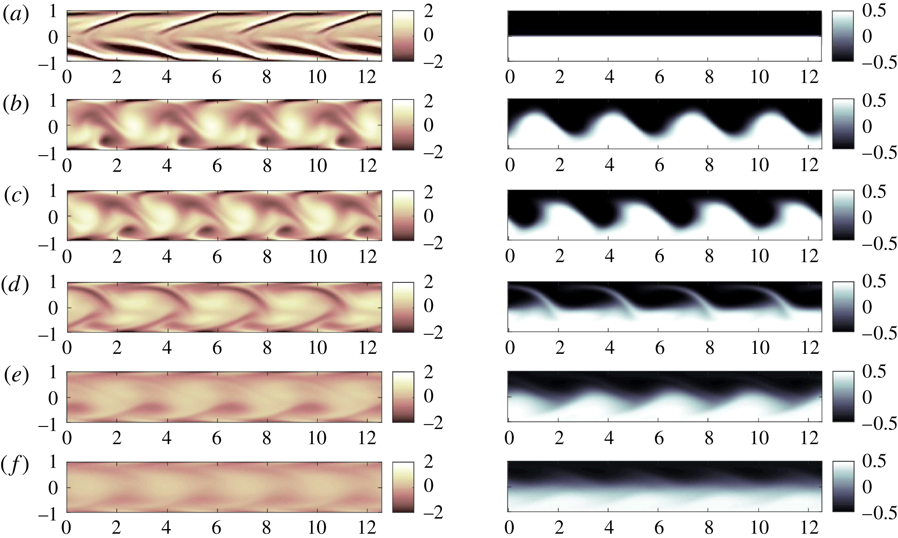
Snapshots of the vorticity field (left-hand column) and density field (right-hand column) for the flow induced by the optimal perturbation for time-averaged perturbation kinetic-energy maximisation with
 $Ri_{b}=0.1$
at times as marked in the left-hand panels of figure 5: from (a–f),
 $T=0$
;
 $T=A=4.5$
;
 $T=B=6.2$
;
 $T=10$
;
 $T=C=20.3$
;
 $T=30$
.
Snapshots of the vorticity field (left-hand column) and density field (right-hand column) for the flow induced by the optimal perturbation for mix-norm minimisation with
 $Ri_{b}=0.1$
at times as marked in the right-hand panels of figure 5: from (a–f),
 $T=0$
;
 $T=A=2.7$
;
 $T=B=6.9$
;
 $T=10$
;
 $T=C=15.7$
;
 $T=30$
.
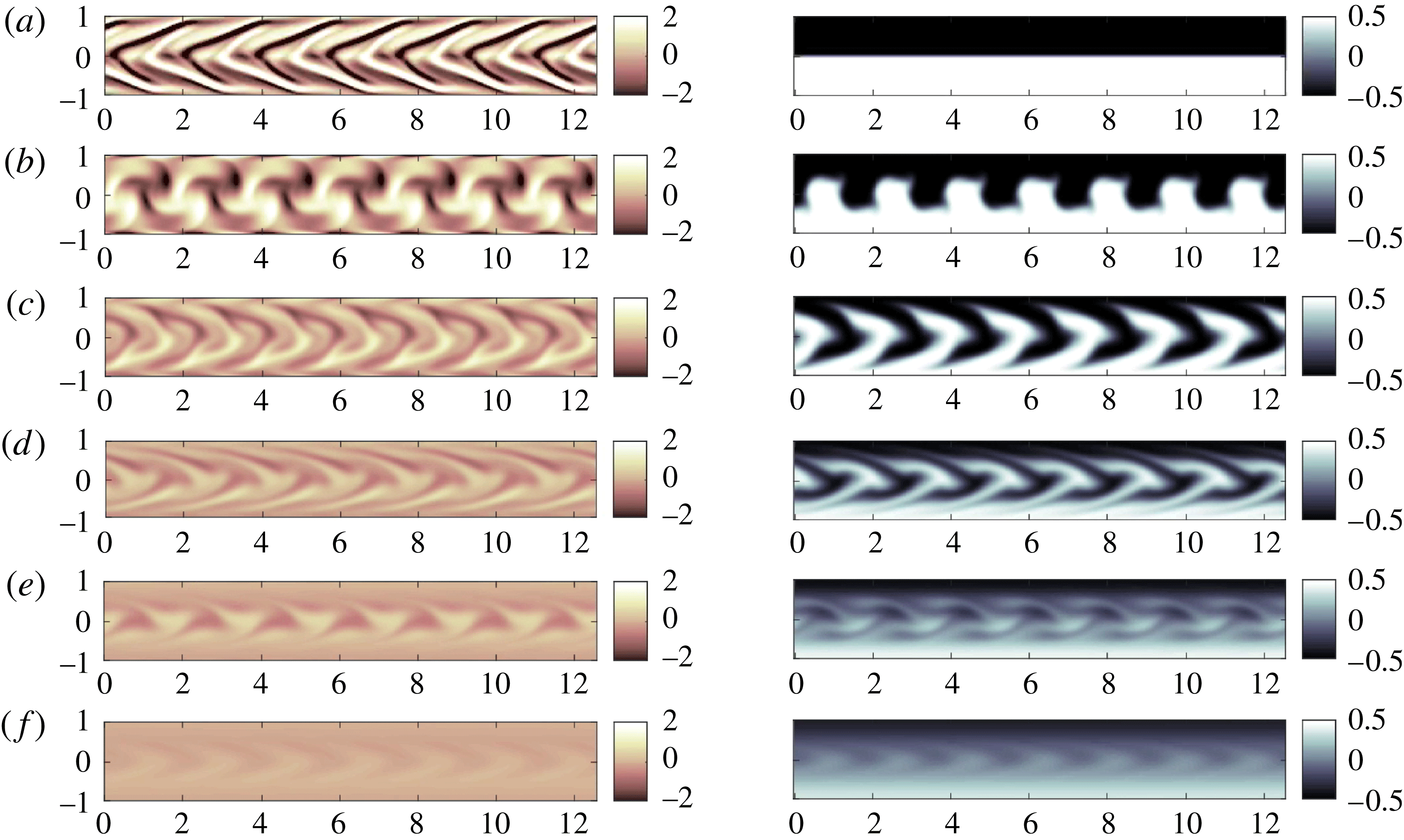
Furthermore, in both flows, most of the conversion from available potential energy to background potential energy occurs between the times marked ‘B’ and ‘C’, subsequent to which the effects of advection-driven irreversible mixing becomes negligible compared to those of purely molecular diffusion. However, the striking difference between the two flows is that in the flow initialised by the optimal perturbation for mix-norm minimisation, (shown in figure 7) the perturbation kinetic energy is markedly smaller. The density field consists of elongated protrusions, tilted by the base flow velocity field to project dense and light fluid filaments into the lower and upper half-planes respectively, aligned with the base velocity. The irreversible mixing occurring afterwards therefore mostly relies on stirring by the base flow rather than the perturbation, taking advantage of Taylor dispersion. It is clear from the snapshots in figure 7 that from time ‘B’, the structure of the density does not experience any significant structural change, but is rather advected by the base flow and smoothed out by diffusion.
Conversely, for the flow associated with the initial perturbation which maximises the time-averaged perturbation kinetic energy, the evolution of the density field during the third phase of flow evolution (i.e. the ‘dispersion’ stage) is strongly affected by stirring (by its nature at least partially reversible) by the still non-trivially energetic perturbation velocity field. This perturbation is central to the creation of the relatively small filamented structures visible in figure 6. Remarkably, the inflection point in the time evolution of the background potential energy in figure 5(a) lies between times
 $t=10$
and
 $t=15$
, indicating that the irreversible mixing rate
 $M$
reaches its maximum in this interval, interestingly slightly after the optimisation time horizon
 $T=10$
. The snapshots shown in figure 6 demonstrate that this maximum in the mixing corresponds to the roll up of these thin, and sparsely distributed protruding filaments becoming subject to the restoring buoyancy force.
4.4 Assessing mixing efficiency
Following Caulfield & Peltier (Reference Caulfield and Peltier2000) and Peltier & Caulfield (Reference Peltier and Caulfield2003), we can now use the inferred irreversible mixing rate
 $M$
introduced in (4.4) to define an appropriate instantaneous mixing efficiency
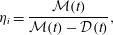 $$\begin{eqnarray}\unicode[STIX]{x1D702}_{i}=\frac{{\mathcal{M}}(t)}{{\mathcal{M}}(t)-{\mathcal{D}}(t)},\end{eqnarray}$$
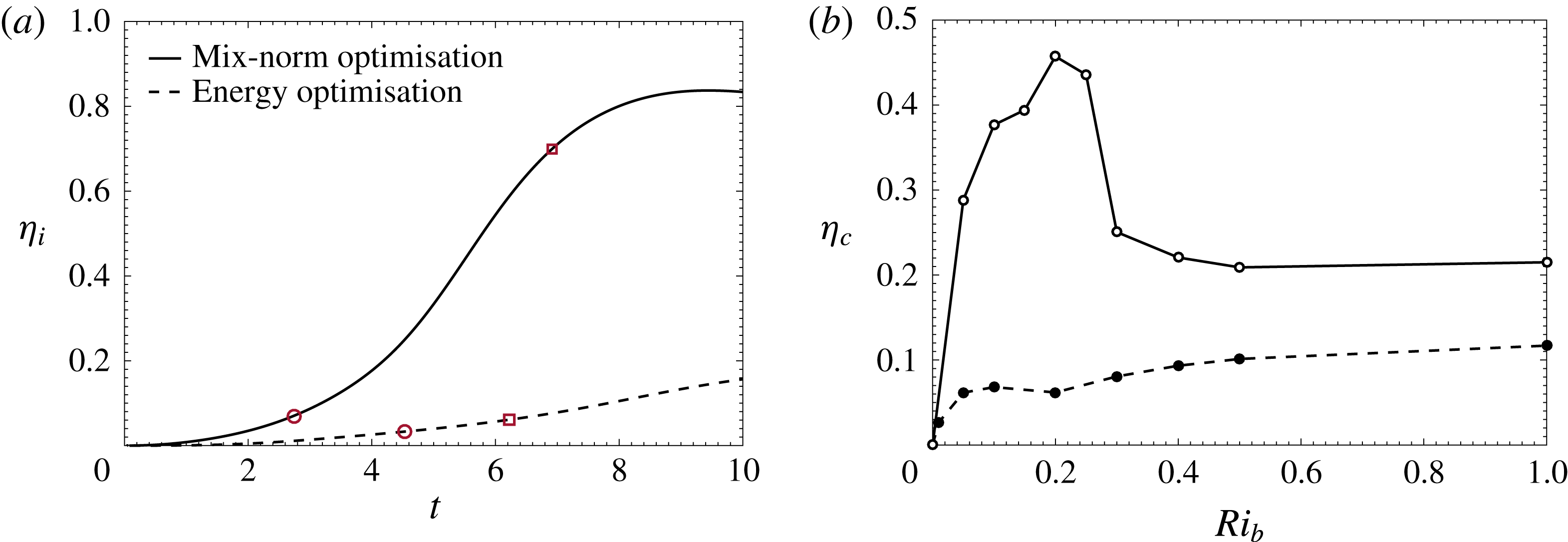
the ratio of the irreversible mixing rate inherently due to fluid motion to the sum of this rate and the viscous dissipation of the perturbation kinetic energy. This instantaneous mixing efficiency, quantifying as it does the proportion of kinetic energy lost by the perturbation that leads to irreversible mixing, has the further attraction of being easily computed at each time step. We plot its time evolution in figure 8(a) as a function of time over the optimisation time interval
 $[0,10]$
, for the same flows with
 $Ri_{b}=0.1$
associated with mix-norm minimisation (plotted with a solid line) and the flow associated with maximisation of the time-averaged perturbation kinetic energy (dashed line).
For the flow associated with mix-norm minimisation,
 $\unicode[STIX]{x1D702}_{i}$
steeply increases between the times ‘A’ and ‘B’ as the total potential energy reaches a plateau at the end of the transport phase, associated with (clearly) efficient exchange of kinetic energy to the potential energy reservoir, coincident also with the available potential energy reservoir emptying and the background potential energy reservoir increasing. For the flow associated with time-averaged kinetic-energy maximisation, the increase in
 $\unicode[STIX]{x1D702}_{i}$
is significantly more modest, reaching an appreciably smaller peak value, illustrating in a different way that this optimisation problem is suboptimal in causing mixing in such a stratified flow.
(a) Time evolution of the instantaneous mixing efficiency
 $\unicode[STIX]{x1D702}_{i}$
(as defined in (4.5)) over the optimisation time horizon
 $[0,10]$
, for flows with
 $Ri_{b}=0.1$
initialised with optimal perturbations for mix-norm minimisation (plotted with a solid line) and for time-averaged kinetic-energy maximisation (dashed line). In both cases times ‘A’ (circles) and ‘B’ (squares) are indicated for reference. (b) Variation with
 $Ri_{b}$
of the cumulative mixing efficiency
 $\unicode[STIX]{x1D702}_{c}$
(as defined in (4.6)) integrated up to time
 $T^{\ast }=30$
, for flows initialised with perturbations for mix-norm minimisation (solid line and empty circles) and time-averaged kinetic-energy maximisation (dashed line and full circles).
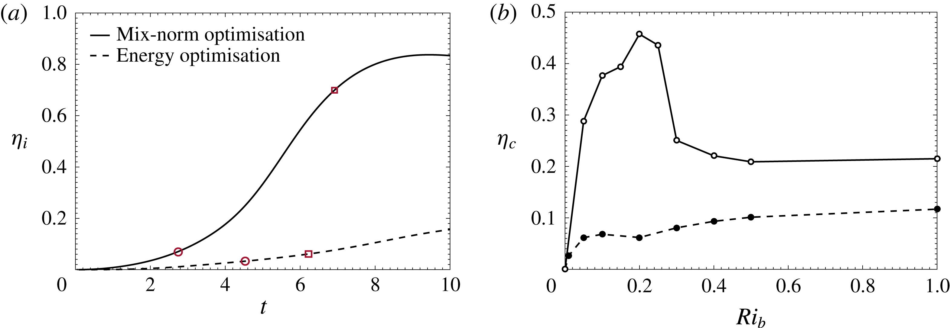
This picture appears to be largely consistent for all the flows we have considered with different
 $Ri_{b}$
. To demonstrate this we calculate an appropriate cumulative mixing efficiency
 $\unicode[STIX]{x1D702}_{c}$
, defined as
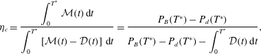 $$\begin{eqnarray}\unicode[STIX]{x1D702}_{c}=\frac{\displaystyle \int _{0}^{T^{\ast }}{\mathcal{M}}(t)\,\text{d}t}{\displaystyle \int _{0}^{T^{\ast }}\left[{\mathcal{M}}(t)-{\mathcal{D}}(t)\right]\,\text{d}t}=\frac{P_{B}(T^{\ast })-P_{d}(T^{\ast })}{\displaystyle P_{B}(T^{\ast })-P_{d}(T^{\ast })-\int _{0}^{T^{\ast }}{\mathcal{D}}(t)\,\text{d}t},\end{eqnarray}$$
where
 $P_{d}(t)$
is the potential energy density associated with the purely diffusive density field
 $\unicode[STIX]{x1D70C}_{d}$
. We plot
 $\unicode[STIX]{x1D702}_{c}$
as a function of
 $Ri_{b}$
in figure 8(b) for the two classes of flows on which we are focussing: those associated with mix-norm minimisation (plotted with a solid line); and those associated with time-averaged perturbation kinetic-energy maximisation (dashed line). These optimisation problems have all been calculated with respect to the ‘intermediate’ time horizon
 $T=10$
, but we set the terminal time in the calculation of
 $\unicode[STIX]{x1D702}_{c}$
to be the ‘long’ time
 $T^{\ast }=30$
.
It should be emphasised that, since
 ${\mathcal{M}}$
is proportional to
 $Ri_{b}$
, mixing efficiency defined in this way inevitably tends to zero in the limit of zero stratification. This measure further highlights the suboptimality of the energy maximising flows for all the considered stratifications. For both optimisation problems, the cumulative mixing efficiency plateaus at higher
 $Ri_{b}$
, with
 $\unicode[STIX]{x1D702}_{c}$
for the mix-norm minimising flows approaching an asymptotic value nearly twice the equivalent asymptotic value for the energy maximising flows. These asymptotic values correspond to flows where the initial perturbation is no longer sufficiently energetic for the filamentary structures to develop adequately and form the ‘stripes’ or ‘chevrons’ necessary to exploit Taylor dispersion and enhance diffusive mixing. Interestingly, and perhaps fortuitously, this asymptotic value
 $\unicode[STIX]{x1D702}_{c}\simeq 0.2$
is quite close to, but slightly larger than the classic bounding value of Osborn (Reference Osborn1980) of the turbulent flux coefficient
 $\unicode[STIX]{x1D6E4}\simeq \unicode[STIX]{x1D702}_{c}/(1-\unicode[STIX]{x1D702}_{c})\leqslant 0.2$
, since for this flow
 $\unicode[STIX]{x1D6E4}_{c}\simeq 0.25$
. However, it is very important to remember that this flow is restricted to evolve in two dimensions, and so the particular quantitative mixing dynamics must be treated with caution.
On the other hand, the noticeable kink in the solid curve for the mix-norm minimising flows around
 $Ri_{b}=0.2$
suggests a particularly favourable flow configuration, consistent with the evolution of the density fields already discussed in § 3.1. For smaller
 $Ri_{b}\lesssim 0.25$
, the base flow shear prevents the ‘chevrons’ from collapsing back to their neutrally buoyant positions, thus allowing the filaments to remain in the near-wall regions of higher shear where Taylor dispersion ensures efficient mixing. Furthermore, for
 $Ri_{b}\simeq 0.2{-}0.25$
, the combined effects of this Taylor dispersion and (significantly) convective overturning result in a peak in mixing efficiency, followed by a relatively rapid drop at slightly higher
 $Ri_{b}$
as the distorted interface is no longer advected close to the boundaries, and so Taylor dispersion no longer occurs.
This maximum value of the mixing efficiency
 $\unicode[STIX]{x1D702}_{c}\simeq 0.4{-}0.5$
with intermediate Richardson number is similarly somewhat reminiscent of the behaviour of transient stratified shear flows prone to Kelvin–Helmholtz instabilities (see for example Mashayek et al.
Reference Mashayek, Caulfield and Peltier2013), although this apparent agreement may of course be coincidental since the inherently two-dimensional flows considered here are neither linearly unstable nor turbulent at any stage. Indeed, it is important to appreciate that the non-monotonic dependence of
 $\unicode[STIX]{x1D702}_{c}$
on
 $Ri_{b}$
is due to the existence of two qualitatively different flow dynamics at smaller and higher
 $Ri_{b}$
, and so should not be interpreted as implying the development of well-mixed layers separated by relatively ‘sharp’ interfaces due to the so-called ‘Phillips mechanism’ (Phillips Reference Phillips1972).
5 Conclusions
Using the direct-adjoint-looping (DAL) method, involving numerical integration of the fully nonlinear direct-adjoint Boussinesq equations, we have for the first time identified initial perturbations which lead to optimal mixing in a density-stratified flow at
 $Re=Pe=500$
. For ease of comparison with Foures et al. (Reference Foures, Caulfield and Schmid2014), the same (effectively) proof-of-concept optimisation problem has been considered. Perturbations of fixed kinetic energy in plane Poiseuille flow driven by a constant base pressure gradient have been identified which (over the chosen intermediate time horizon
 $T=10$
) either maximise the time-averaged perturbation kinetic energy, or minimise the ‘mix-norm’ quantifying the homogenisation of the flow.
Consistently with the passive scalar flow results of Foures et al. (Reference Foures, Caulfield and Schmid2014), the flows associated with both optimisation problems exploit first an ‘Orr mechanism’ for transferring kinetic energy from the base Poiseuille flow to the perturbation (leading to ‘transport’ of the scalar into a ‘stripes’ or ‘chevrons’ structure) followed by Taylor dispersion which leads to enhanced diffusive fluxes before both flows eventually ‘relax’ through simple diffusion. Nevertheless, for all stratifications, the flows associated with mix-norm minimisation are substantially less energetic than the flows associated with energy maximisation, yet substantially more effective at reducing the (dynamic) scalar variance. This difference is particularly marked for moderate values of the bulk Richardson number (
 $Ri_{b}\sim 0.2$
) as stratification especially inhibits the development of the large-scale, wavy structures characteristic of flows which maximise the time-averaged perturbation kinetic energy.
Comparison of the time evolution of the kinetic energy and the various potential energies associated with each of the optimisation problems shows that although the transient growth in the perturbation kinetic energy is significantly higher for the time-averaged kinetic-energy maximisation flows, the potential energy exhibits much larger ultimate growth with the mix-norm minimisation flows. This phenomenon indicates that the development of the particular perturbations in such flows is much more effective at inducing irreversible mixing through modification of the initial density distribution at small scales. The mix-norm minimising optimal perturbations prove reliable in identifying a particular type of stirring mechanism with two key characteristics. First, the stirring rapidly stores a large amount of available potential energy once the perturbation kinetic energy has reached its maximum value. Second, the stirring then converts this available potential energy, essentially in one shot, into background potential energy, without the characteristic oscillatory, and at least partially reversible, exchange between the kinetic energy and potential energy reservoirs typical of flows which maximise time-averaged perturbation kinetic energy.
Our stratified, yet still highly idealised, results constitute further evidence that variational optimisation problems focussed on mix-norm minimisation provide robust and computationally efficient indicators to identify dynamical processes that ensure scalar mixing, even in flows with buoyancy forces. Specifically, for all the values of
 $Ri_{b}$
we consider, we demonstrate that mix-norm minimisation over intermediate times remains a robust and computationally efficient proxy for variance minimisation (i.e. thorough mixing) over long times. This observation suggests two interesting open questions for future consideration. First, how short can such an ‘intermediate’ time be taken for the mix-norm minimising optimal perturbations still to be adequately close to the (desired) long-time variance minimising perturbations? A second, potentially more general question, is whether there is an ‘optimal’ mix-norm, in the sense of a specific (negative) index of a Sobolev norm for which the associated minimisation problem is the most robust and computationally efficient proxy for identification of long-time optimal variance minimising perturbations, which are typically the perturbations of most relevance.
As the nonlinear DAL method which we have used here is somewhat computationally demanding, we have here restricted our attention to a two-dimensional flow in a simple streamwise periodic geometry, well below the linear stability threshold, with
 $Pr=1$
. These assumptions obviously strongly restrict quantitative application, but in principle the same techniques can be used to consider three-dimensional flows at higher
 $Re$
and
 $Pr$
, as in Vermach & Caulfield (Reference Vermach and Caulfield2018).
Indeed, this method has the potential to address some fundamental outstanding questions in (turbulent) stratified mixing, not least of which is the question of whether the mixing associated with classic, and widely studied flow instabilities (such as the Kelvin–Helmholtz instability) is actually ‘optimal’. Although there is some evidence (see for example Mashayek et al. Reference Mashayek, Caulfield and Peltier2017) that the initial large-scale overturning associated with this instability is particularly conducive to efficient mixing, the methodology presented here can be straightforwardly formulated to investigate whether other perturbations might be even more effective at mixing.
In a more industrial context, as also demonstrated by Foures et al. (Reference Foures, Caulfield and Schmid2014), the underlying optimisation problem can be formulated to identify not an optimal initial perturbation, but rather an optimal wall forcing strategy to encourage mixing. What is the best forcing strategy with a constrained power for a stratified fluid in a constrained geometry is obviously an interesting question. Since our results suggest that maximising perturbation energy may well be suboptimal, it is at least possible that the optimal forcing strategy may be counter-intuitive, and may not rely (or indeed require) substantial injections of energy, which would have the potential for non-trivial savings in the (total) energy cost required to mix fluids effectively to a required tolerance.
Acknowledgements
F.M. was funded by a David Crighton Fellowship from the Department of Applied Mathematics and Theoretical Physics at the University of Cambridge. The research activity of C.P.C. is supported by the EPSRC Programme Grant EP/K034529/1 entitled ‘Mathematical Underpinnings of Stratified Turbulence’. Both authors wish to thank P.J. Schmid for many fruitful discussions and D.P.G. Foures for providing a version of the DAL method code described in Foures et al. (Reference Foures, Caulfield and Schmid2013). Furthermore, the constructive comments of anonymous referees have significantly improved the clarity and presentation of our results. The codes and initial conditions used to generate all the data used in the figures are available at doi:10.17863/CAM.25375.
Supplementary movies
Supplementary movies are available at https://doi.org/10.1017/jfm.2018.565.