





1. Introduction
Drag reduction by air lubrication is one of the techniques applied to reduce frictional resistance beneath a ship’s hull. Despite the fact that this technology has already been extensively studied and implemented on ships, the physical mechanisms responsible for drag reduction are still not fully understood. As a result, discrepancies persist between model-scale and full-scale results, and reliable scaling laws have yet to be established. This is partly due to the complex multiphase nature of these flows and the difficulty of performing experiments or numerical simulations at the high Reynolds numbers relevant to full-scale conditions. Better understanding of these flows could lead to improved designs of air lubrication systems that target specific operating conditions.
In the literature, these flows are mostly studied by means of injecting air into the spatially developing turbulent boundary layer (TBL) of a flat plate. In most of these studies a backward-facing step or cavitator is used upstream of the air injector (Zverkhovskyi Reference Zverkhovskyi2014; Barbaca et al. Reference Barbaca, Pearce, Ganesh, Ceccio and Brandner2019). While this insert is shown to enhance the stability of the air phase, it demands an additional hull modification on existing ships. Another option is to inject air into the TBL without the use of such inserts, a configuration much less researched (Elbing et al. Reference Elbing, Winkel, Lay, Ceccio, Dowling and Perlin2008; Jang et al. Reference Jang, Choi, Ahn, Kim and Seo2014; Nikolaidou et al. Reference Nikolaidou, Laskari, van and Poelma2024).
With this configuration, three air phase regimes are commonly observed. For a constant free-stream velocity (
 $U_{\infty }$
) and for small air flow rates (
 $Q_{\textit{air}}$
), a bubbly regime (BR) is observed. In this regime, dispersed bubbles are present in the flow. By further increasing
 $Q_{\textit{air}}$
, the bubbles coalesce to form air patches (transitional air layer regime – TALR). Eventually by further increasing
 $Q_{\textit{air}}$
, the air patches also coalesce and an air layer is formed (air layer regime – ALR). Elbing et al. (Reference Elbing, Winkel, Lay, Ceccio, Dowling and Perlin2008) performed large-scale air lubrication experiments in a
 $13$
m long flat plate, where the shear stress was measured over several locations downstream of a slot-type injector. They defined each regime based on the resultant drag reduction (DR). More specifically, the TALR and the ALR were demarcated by 20 % and 80 % DR, respectively. This was based on a single
 $U_{\infty }$
measurement and a single shear stress measurement location. These measurements revealed a steep increase in DR with
 $Q_{\textit{air}}$
within the TALR (
 $20\,\%\lt \textrm{DR}\lt 80\,\%$
) followed by a gradual convergence towards nearly 100 % DR as
 $Q_{\textit{air}}$
increased further within the ALR. In our previous study (Nikolaidou et al. Reference Nikolaidou, Laskari, van and Poelma2024), using a similar air injector to Elbing et al. (Reference Elbing, Winkel, Lay, Ceccio, Dowling and Perlin2008), we also found all three regimes with a similar morphology, but no quantitative comparison with Elbing et al. (Reference Elbing, Winkel, Lay, Ceccio, Dowling and Perlin2008) was possible in the absence of drag force measurements. While Elbing et al. (Reference Elbing, Winkel, Lay, Ceccio, Dowling and Perlin2008) performed experiments in a large range of conditions spanning all three air phase regimes, their focus was not on the physical mechanisms of DR. In the following sections, we discuss the DR mechanisms associated with the BR, TALR and ALR separately, based on insights from other existing literature.
Many studies have targeted the
 $\textrm{BR}$
and explored the DR mechanisms following the successful results of microbubble DR (McCormick & Bhattacharyya Reference McCormick and Bhattacharyya1973). As a result, earlier studies have focused particularly on microbubbles (e.g. Ferrante & Elghobashi Reference Ferrante and Elghobashi2004; Sanders et al. Reference Sanders, Winkel, Dowling, Perlin and Ceccio2006; Elbing et al. Reference Elbing, Winkel, Lay, Ceccio, Dowling and Perlin2008). In contrast, the effects of larger, millimetre-sized bubbles have received comparatively less attention. Across these studies, DR mechanisms are generally attributed to modifications of the momentum transfer in the near-wall region, such that the drag is reduced. A broad consensus highlights bubble deformability – captured by the Weber number – as the main parameter governing DR (Lu et al. Reference Lu, Fernández and Tryggvason2005; Kim & Moin Reference Kim and Moin2010; Van Gils et al. Reference Van, Dennis, Guzman, Sun and Lohse2013; Verschoof et al. Reference Verschoof, van der Veen, Sun and Lohse2016). Murai (Reference Murai2014) summarised the successful DR regimes in a bubble diameter –flow speed plot. He suggested a classification of the mechanisms by looking into the bubble sizes in comparison with the coherent structures. He notes that DR can be achieved either by small bubbles (
 $\unicode{x03BC}{\rm m} -{\rm mm}$
) in high-speed flows (
 ${\gt } 1$
m s–1) or larger bubbles (
 ${\rm mm}$
) in low-speed flows (
 ${\lt } 0.1$
m s–1). For velocities in between these two regimes, bubbles smaller than one centimetre are increasing the drag by perturbing the laminar state and triggering flow transition. Yet, results of an increase in drag due to bubbles are relatively scarce in the literature. Henry et al. (Reference Henry, Savio, Koushan, Jenssen, Hanssen and Brink2023) performed air lubrication measurements on a flat plate over smooth and rough surfaces. A drag increase was reported for
 $U_{\infty }=2$
m s–1 and the lowest air flow rates tested within the BR. No information on the corresponding bubble size was reported. These drag-increasing bubbles were measured to travel at approximately
 $0.5U_{\infty }$
while the relative bubble speed increased with increasing
 $U_{\infty }$
, suggesting that, for higher
 $U_{\infty }$
, bubbles might migrate at the outer layer of the TBL. Biswas & Govardhan (Reference Biswas and Govardhan2024) performed experiments in shallow channel flow, with and without salts, at relatively low Reynolds numbers. They saw that smaller bubbles (as a result of salt addition) result in drag increase. They attributed this effect in smaller bubbles being less deformable due to their more spherical size and also due to the deposition of salt ions at the bubble/water interface. They noticed that smaller bubbles stay densely packed and close to the top wall, unlike the smaller salt-born bubbles which disperse near the top wall. Bubble drag increase was also found by Gabillet et al. (Reference Gabillet, Colin and Fabre2002). In that experiment, bubbles were injected from a porous layer in the bottom wall of a channel, rising to the top one. It is shown that, close to the (bottom) wall, near the injection, bubbles are of the same size as the energy containing eddies and successfully modify near-wall turbulence, while the liquid flow profile behaves like a rough TBL with the roughness parameter correlating with bubble size. Hori (Reference Hori2024) performed interface-resolving direct numerical simulations on a bubbly plane-Couette flow for low friction Reynolds number
 $Re_{\tau }$
. The effect of bubbles and air layers on the drag force was investigated by varying the Weber and Froude numbers for moderate volume fractions of air (1 %–5 %). They found that, in small Weber and high Froude number cases, bubbles increase drag with respect to the single-phase flow. By decomposing the stresses in contributions of advection, diffusion and interfacial tension, they found that in these drag-increasing cases, there is a large contribution from the interfacial tension term, which enhances momentum transfer.
Within the TALR, larger air patches are formed. This regime is largely unexplored with only a few instances in the literature (Jang et al. Reference Jang, Choi, Ahn, Kim and Seo2014; Nikolaidou et al. Reference Nikolaidou, Laskari, van and Poelma2024). No conclusive information on the DR mechanisms is reported, but it is hypothesised that DR comes directly from the reduction of wetted area. Regarding the ALR, the same hypothesis holds. At the same time, it is shown that this regime is sensitive to upstream disturbances from the incoming TBL (Elbing et al. Reference Elbing, Mäkiharju, Wiggins, Perlin, Dowling and Ceccio2013). Similarly, in Nikolaidou et al. (Reference Nikolaidou, Laskari, van and Poelma2024) it was found that the incoming TBL conditions affect both the onset of the ALR and also the air layer topology: bigger air layer thickness to incoming TBL thickness ratios result in an earlier onset of ALR and a larger air layer length. In addition, local, instantaneous incoming TBL organisation also governs break up of the air layer close to the injector (Laskari Reference Laskari2025).
Since the
 $\textrm{ALR}$
is the desired regime in terms of DR, special attention has been given in the literature to the critical air flow rate
 $Q_{\textit{crit}}$
, the one needed for an air layer to be formed. While it has been shown that
 $Q_{\textit{crit}}$
increases with
 $U_{\infty }$
, only a few scaling attempts have been reported. In Elbing et al. (Reference Elbing, Mäkiharju, Wiggins, Perlin, Dowling and Ceccio2013) a potential scaling of the
 $Q_{\textit{crit}}$
is proposed by analysing a single bubble, subjected to shear flow. This scaling indicates that the transition to ALR depends on the ratio of buoyancy to turbulent shear forces, with buoyancy promoting phase separation and turbulent fluctuations enhancing phase dispersion. While a good collapse of most results was exhibited, the authors suggest it is not conclusive and should be regarded as a starting point for further work on the onset of ALR (Elbing et al. Reference Elbing, Mäkiharju, Wiggins, Perlin, Dowling and Ceccio2013). Scaling of the
 $Q_{\textit{crit}}$
is also discussed in Peifer et al. (Reference Peifer, Callahan-Dudley and Mäkiharju2020), where the authors adopt the following approach: they assume that an air layer is formed and hypothesise that interfacial instabilities – such as Kelvin–Helmholtz waves and turbulent fluctuations – act to wet the surface. They therefore propose that the frequency of wetting events depends on both the outer liquid flow characteristics and the thickness of the air layer. Despite these efforts, there is still no scaling of the critical air flow rate that captures all phenomena and further tests are needed.
While the aforementioned experiments span a wide range of conditions, a parameter not highlighted enough is the depth of the experimental facility and its potential effect on the air phase topology and dynamics. In the case of the ALR, a free surface is present between the air layer and the surrounding liquid. Using the liquid free-stream velocity
 $U_{\infty }$
and the water depth
 $d$
, a Froude-depth number,
 $\textit{Fr}_d$
, can be defined as
 \begin{align} Fr_d=\frac {U_{\infty }}{\sqrt {gd}} .\end{align}
Only a limited number of studies explicitly address the role of
 $\textit{Fr}_d$
. Barbaca et al. (Reference Barbaca, Pearce, Ganesh, Ceccio and Brandner2019) reported a change in cavity closure behaviour and hypothesised that it was related to variations in
 $\textit{Fr}_d$
. In contrast, Mäkiharju et al. (Reference Mäkiharju, Elbing, Wiggins, Schinasi, Vanden-Broeck, Perlin, Dowling and Ceccio2013), who conducted measurements exclusively in the supercritical regime (
 $\textit{Fr}_d \gt 1.4$
), suggested that the cavity closure mechanism should remain similar at lower Froude numbers, since the dominant parameters (
 $U_{\infty }$
, fluid properties and closure configuration) remain unaltered with
 $\textit{Fr}_d$
. In most studies, due to the limited depth of facilities,
 $\textit{Fr}_d\gt 1$
such that the flow is supercritical, analogous to the supercritical open channel flow regime (Sanders et al. Reference Sanders, Winkel, Dowling, Perlin and Ceccio2006; Elbing et al. Reference Elbing, Winkel, Lay, Ceccio, Dowling and Perlin2008; Elbing et al. Reference Elbing, Mäkiharju, Wiggins, Perlin, Dowling and Ceccio2013; Mäkiharju et al. Reference Mäkiharju, Elbing, Wiggins, Schinasi, Vanden-Broeck, Perlin, Dowling and Ceccio2013). In these studies, although imaging of the air phase is not performed, it is stated that once the air layer is formed it covers the total length of the flat plate. Only few studies exist within the subcritical regime yielding
 $\textit{Fr}_d\lt 1$
(Zverkhovskyi Reference Zverkhovskyi2014; Nikolaidou et al. Reference Nikolaidou, Laskari, van and Poelma2024). For this regime, it has been shown, using potential flow theory, that a stable cavity length exists and can be predicted by the dispersion relation (Butuzov Reference Butuzov1966, Reference Butuzov1967; Matveev Reference Matveev2003). More specifically, for deep water conditions (approximately
 $\textit{Fr}_d\lt 0.61$
), it has been shown that the air cavity length is in good agreement with half a gravity wave predicted by the dispersion relation (Qin et al. Reference Qin, Wu, Wu and Hong2019; Nikolaidou et al. Reference Nikolaidou, Laskari, van and Poelma2024). However, no systematic analysis of the influence of
 $\textit{Fr}_d$
has been conducted, and this constitutes one of the main objectives of the present work.
In order to investigate the potential effect of
 $\textit{Fr}_d$
on the air phase topology, imaging data are required. Past experimental studies have typically focused on measuring drag forces (Sanders et al. Reference Sanders, Winkel, Dowling, Perlin and Ceccio2006; Elbing et al. Reference Elbing, Winkel, Lay, Ceccio, Dowling and Perlin2008), while imaging data are often limited to the BR (for bubble sizes) in a few conditions, or targeted in the closure region (Elbing et al. Reference Elbing, Mäkiharju, Wiggins, Perlin, Dowling and Ceccio2013; Mäkiharju et al. Reference Mäkiharju, Elbing, Wiggins, Schinasi, Vanden-Broeck, Perlin, Dowling and Ceccio2013) of the air layer. The global morphology of the air phase regime is rarely captured. On the other hand, imaging of the air phase topology by means of high-speed imaging or X-ray densitometry (Barbaca et al. Reference Barbaca, Pearce, Ganesh, Ceccio and Brandner2019; Qin et al. Reference Qin, Wu, Wu and Hong2019; Gawandalkar et al. Reference Gawandalkar, Lucido, Jain, Poelma, Ceccio and Ganesh2025) have been used to gain insight to the air phase topology of similar flows. However, no studies exist that combine both drag force measurements and imaging of the global air phase topology.
In this paper, simultaneous measurements of the drag force acting on a flat plate TBL and imaging of the air phase regimes are performed. The latter allows us to probe the air phase topology and perform qualitative as well as quantitative analyses as needed for the air phase characteristics. By combining them with drag measurements, we aim to gain physical insight into the mechanisms responsible for DR. To that end, the air flow rate, free-stream velocity and Froude-depth number are systematically varied, allowing a wide range of air phase regimes to be investigated and general trends to be identified. These are discussed and compared for different
 $\textit{Fr}_d$
conditions (subcritical and supercritical) to fill in the aforementioned knowledge gap in this context.
The remainder of this paper is organised as follows. In § 2 the experimental set-up and methods are given. In § 3 the single-phase flow parameters of a developing TBL along a flat plate are given which are then used to evaluate the influence of air. Sections 4 and 5 describe the multiphase flow results associated with
 $\textit{Fr}_d \gt 1$
and
 $\textit{Fr}_d \lt 1$
, respectively. In § 6 all results are combined in a single air phase regime map and scaling considerations of the critical air flow rate are presented.
2. Experimental set-up and methods
2.1. Facility
The experiments were performed in the new multiphase flow tunnel (MPFT) at the Ship Hydromechanics laboratory of Delft University of Technology. The flow is driven by a Voith Inline Thruster (Voith, Heidenheim, Germany) resulting in low noise and vibrations. The operational range of the impeller leads to free-stream velocities
 $U_{\infty }$
= 2.13–13 m s–1 and with the addition of an orifice plate downstream of the rim-driven thruster, a minimum
 $U_{\infty }$
= 0.5 m s–1 can be reached. To facilitate air lubrication experiments, the MPFT features two kind of degassing mechanisms to prevent air circulation: a de-aeration tower and a large horizontal degasser (figure 1). In the de-aeration tower, the air–water mixture impacts a sloped plate that breaks air patches, allowing air to escape via a separation vessel, while water flows downstream. The horizontal degasser features a specially designed top lid that collects rising bubbles and directs them to the separation vessel. The former degassing mechanism is mainly effective for lower velocities (
 ${\lt } 3$
m s–1) and the latter for higher ones. Before entering the test section the flow is conditioned with a honeycomb and two contractions (figure 1) to ensure a uniform inflow and low turbulence intensity (
 ${\lt}0.6\,\%$
as measured by Laser Doppler Anemometry (LDA), see Nikolaidou et al. Reference Nikolaidou, Laskari, van Terwisga and Poelma2026).
Sketch of the multiphase flow tunnel. Arrows indicate the liquid flow direction. For an indication of the scale: the test section is 2.1 m long.

Figure 1. Long description
A diagram of a multiphase flow tunnel. The diagram includes a de-aeration tower, separation vessel, large contraction, small contraction, honeycomb, test section, differential pressure sensor, temperature sensor, large degasser, and inline thruster housing. Arrows indicate the liquid flow direction through these components. The test section is 2.1 meters long.
The test section is 2.136 m long and the cross-section varies from 0.3
 $\times$
0.3
 ${\rm m}^2$
at the inlet to
 $0.3 \times 0.32$
 ${\rm m}^2$
at the outlet due to a sloping bottom. The sloping bottom was designed to compensate for the TBL growth for 2 m s–1. The test section is tightly sealed with a lid, and it can be pressurised up to 2 bar overpressure. Transparent windows are present on the sides of the tunnel and the bottom, while the top has limited access with 4 viewing windows. The water level in the test section can be monitored with a transparent tube and is kept constant throughout the experiments.
2.2. Test plates
Two different test plates were used during the experiments, one for single-phase flow and one for air lubrication measurements. The former was a simple flat plate without inserts, used to measure the TBL flow for validation of our measurement system (see § 3). The air lubrication plate was more complex and was subsequently used for multiphase flow measurements (see §§ 4 and 5). The test plates were positioned flush with the ceiling of the test section and were submerged in water (depth
 $d=0.3$
m). Both were made out of transparent polycarbonate, with length
 $L=1.95$
m and width
 $B=0.295$
m. The thickness was 11 and 36 mm (in 3 layers of 12 mm) for the single-phase and air lubrication plates, respectively. A zig-zag strip of 0.8 mm thickness was placed 10 cm upstream of the leading edge of the test plates in the tunnel contraction to ensure a TBL.
Sketch of the air injector. (a) Three-dimensional view from the top and (b) side view. Liquid flow is from right to left.

In the case of the air lubrication plate, air was introduced vertically from the top layer through four manifolds equally spaced along the plate’s width (see figure 2). It was then dispersed in an air box within the second layer, whose downstream end was fitted with a porous material and flow conditioner, ensuring homogeneous distribution. At the last layer, air was injected vertically into the liquid TBL via a
 $t=4$
mm wide slot-type injector (same as in our previous work Nikolaidou et al. (Reference Nikolaidou, Laskari, van and Poelma2024)), spanning the width of the plate and located 140 mm downstream of its leading edge. The last layer of the plate was also fitted with side fences along its length (2 mm thick and 49 mm in height) to restrict air escaping from the sides (see figure 3). Within the plate’s middle layer an in-house made LED panel was placed downstream of the injection slot (in a watertight housing) to illuminate the entire plate length and width downstream of the injector, as required for the imaging system (see § 2.4).
The air injection was controlled via a mass flow controller (Bronkhorst EL-FLOW Select series) located several metres upstream of the injector location along with an air filter. The flow meter was factory calibrated for a nominal air flow range of 4–500
 $\textrm{l}$
min–1 with an accuracy of
 $\pm$
0.5 % error in the reading value and
 $\pm$
0.1 % of the full range while the repeatability is 0.2 % of the measured value.
2.3. Drag force measurement system
Both test plates were fitted to a drag force measurement system during their respective uses. This custom-made force balance was designed and built to assess the total friction force of the lower surface of the test plate. The design was based on previously established ones (Zverkhovskyi Reference Zverkhovskyi2014). A load cell (type BM6A by Zemic) with a maximum capacity of 6 kg (
 $60\, \textrm{N}$
) was used. The cell was made from IP68 stainless steel and was suitable for underwater applications both in fresh and salt water.
Sketch of drag force measurement system attached to the air lubrication plate.

The test plate was suspended by four vertical rods, with their top end fixed to the tunnel sidewalls and their bottom attached to longitudinal bars supporting the plate over its length (see figure 3). This allowed plate motion only in the flow direction with alignment screws enabling precise levelling (angle of attack
 $\pm 1^\circ$
). The streamwise displacement of the plate was measured by the load cell, mounted 370 mm from its leading edge. The plate’s width and length were adjusted to maintain a 1.5 mm gap between the plate and the tunnel walls to allow movement and avoid interference. For the air lubrication plate, apart from the side fences, a plastic film at the trailing edge was also used to prevent air from escaping through that gap.
The force balance had to be calibrated in situ. In operating conditions the test section was closed from the top (see figure 1) and filled with water to the brim, resulting in the sensor being fully submerged in water. The calibration was performed without the lid, but with water on top of the plate and the sensor being underwater. Once the lid was closed, the experiments took place and in the end the calibration was repeated to ensure that nothing changed in the system in between. The calibration was performed using standard forces (weights) and a pulley arrangement in accordance to the guidelines given by the ITTC (2017). The calibration involved 16 steps in total of loading and unloading conditions raging from zero to 55 N with a preload as well. A linear relation was found between the output signal in volts and the force in Newtons, with a small standard error (
 $\sigma = 6.9 \times 10^{-3}$
 $\rm V$
, equivalent to 0.0018
 $\rm N$
).
2.4. Imaging system
For the air lubrication measurements, two different imaging systems were used, to accommodate two different research objectives. First, we wanted to capture the three-dimensional air phase topology synchronously with the measured drag force, in order to gain insights into the different DR mechanisms. This necessitated multiple plane views (
 $x{-}y$
,
 $x{-}z$
; see figure 4
a for the coordinate system used), high resolution and thus smaller fields of view (FOVs). Second, we wanted to associate the measured drag force with the total air covered plate area, and probe their correlation. This required large FOVs on the
 $x{-}z$
plane (see figure 4
b).
Camera set-up 1 details.

Table 1. Long description
A table summarizing camera set-up 1 details for air lubrication measurements. The table has four rows and five columns. Column headers are Camera no., FOV (mm x mm), Focal length (mm), f #, and Resolution (px mm^-1). Row 1: Camera no. 1, FOV 740 x 740, Focal length 24, f # 5.6, Resolution 2.75. Row 2: Camera no. 2, FOV 110 x 110, Focal length 105, f # 5.6, Resolution 18.48. Row 3: Camera no. 3, FOV 70 x 70, Focal length 105, f # 5.6, Resolution 30.16.
Imaging systems used for the multiphase flow campaign. (a) Camera set-up 1. (b) Camera set-up 2.

Figure 4. Long description
Panel A: A diagram of camera set-up 1. The setup includes three cameras labeled Camera 1, Camera 2, and Camera 3. An air-injection system is positioned above a flat plate. The side field of view (FOV) and LED lighting are indicated. The flow direction is shown moving from right to left. The coordinate axes x, y, and z are marked. Panel B: A diagram of camera set-up 2. Similar to set-up 1, it includes three cameras labeled Camera 1, Camera 2, and Camera 3. An air-injection system is positioned above a flat plate. The flow direction is shown moving from right to left. The coordinate axes x, y, and z are marked.
Three Imager Pro X 4M cameras (10-bit, LaVision) with a pixel size of 7.4
 $\unicode{x03BC} {\rm m}$
and a resolution of 2048
 $\times$
2048 pixels were used for both set-ups in different configurations and with different lenses, as described below. For wall-parallel imaging planes, illumination was provided by the aforementioned LED panel built within the test plate, while wall-normal imaging was back lit by another LED panel resting on the tunnel sidewall (see figures 2 and 4
a, respectively). Davis 10.2 (LaVision GmbH) was used for data acquisition.
For the first set-up, camera 1 was positioned in a down-up configuration imaging the
 $x{-}z$
plane downstream of the injection slot. This camera provided information on the global air phase characteristics. Camera 2 captured a smaller FOV of the same plane with an increased spatial resolution. Images from this camera were used for estimating smaller features (e.g. bubble sizes). Lastly, a third camera (camera 3) capturing the
 $x{-}y$
plane was used to estimate the bubbly/air layer thickness. This camera was placed in the middle of the test section, except for some tests where it was traversed close to the air injector. All three cameras were synchronously capturing independent snapshots with an acquisition frequency of 0.8–7.4 Hz depending on the
 $U_{\infty }$
. For this campaign
 $U_{\infty }$
varied from 0.5 to 5.5 m s–1, and
 $Q_{\textit{air}}$
from 5 to 400 l min–1. Details of this camera set-up are given in table 1.
For the second set-up, the same three Imager Pro X 4M cameras were used, but in a different configuration. They were positioned below the test section in a down-up configuration to collectively capture the total
 $x{-}z$
extent of the test plate downstream of the injection slot. A small overlap between the three FOVs was present to allow stitching. The acquisition frequency varied from 1.11 to 1.94 Hz depending on
 $U_{\infty }$
, to ensure statistically independent snapshots, whose total number varied from 1000 to 1500. In this campaign
 $U_{\infty }$
was 2 m s–1 and
 $Q_{\textit{air}}$
varied from 5 to 140 l min–1. The exposure time was set to 200
 $\unicode{x03BC} {\rm s}$
to achieve less than one pixel motion blur. Details of this camera set-up are given in table 2.
Camera set-up 2 details.

Table 2. Long description
A table summarizing camera set-up 2 details for three cameras. The table has four columns and three rows. Column headers are Camera no., FOV (mm x mm), Focal length (mm), f#, and Resolution (px mm^-1). Row 1: Camera no. 1, FOV 510 x 510, Focal length 35, f# 4, Resolution 4. Row 2: Camera no. 2, FOV 490 x 490, Focal length 35, f# 4, Resolution 4.22. Row 3: Camera no. 3, FOV 780 x 780, Focal length 24, f# 4, Resolution 2.61.
2.5. Experimental program and procedure
Two experimental campaigns were performed. First, single-phase flow measurements of the drag force acting on the flat plate were performed for a free-stream velocity range of 2–7 m s–1. These included drag force measurements of the flat plate without imaging. Secondly, single and multiphase flow measurements of the drag force acting on the air lubrication plate were performed with synchronous imaging of the air phase. For this campaign the two imaging systems described above were used. First, a short campaign was performed using camera set-up 2. Secondly, measurements using camera set-up 1 were performed. A summary of the experimental conditions for the latter is given in table 3.
Experimental parameters of the multiphase flow campaign using camera set-up 1.

Table 3. Long description
The table presents experimental parameters for a multiphase flow campaign using camera set-up 1. It has five rows and five columns. The columns are labeled Parameters, Definition, Value, and Units. The parameters listed are Free-stream velocity, Air flow rate, Reynolds number, Froude-depth number, and Non-dimensional air flux. The values and units for each parameter are provided. For example, Free-stream velocity ranges from 0.5 to 7 meters per second, Air flow rate ranges from 5 to 450 liters per minute, Reynolds number ranges from 1 to 14 times 10 to the power of 6, Froude-depth number ranges from 0.29 to 4, and Non-dimensional air flux ranges from 0.012 to 1.4.
For a given free-stream velocity, the mean drag force was recorded at 100 Hz and averaged over 10 minutes, which was sufficient for convergence. Simultaneously, the differential pressure across the contraction and the water temperature (as shown in figure 1) were recorded and averaged. The differential pressure was used to estimate
 $U_{\infty }$
, with a correction applied, as set by earlier LDA measurements (Nikolaidou et al. Reference Nikolaidou, Laskari, van Terwisga and Poelma2026). The signals were continuously recorded via LabVIEW. For the multiphase cases, measurements were first performed without air followed by those with air, the mass flow rate of which was also recorded and averaged.
3. Single-phase flow
In this section, single-phase flow results are presented in the absence of air injection. Firstly, the characteristics of the single-phase TBL developing along the flat plate are given. Secondly, the drag force measurement system is validated against theoretical predictions. These will set the baseline for the multiphase flow measurements introduced later.
3.1. Flat plate TBL characterisation
The flat plate TBL thickness was measured with LDA (Nikolaidou et al. Reference Nikolaidou, Laskari, van Terwisga and Poelma2026) in three streamwise locations along the plate and multiple velocities (see table 4 for one
 $U_{\infty }$
). Due to the sloping bottom of the test section, the free-stream velocity was found to slightly decrease at the most downstream position (
 $\approx$
2 %). Due to the position of the flat plate at the tunnel’s ceiling, the TBL was found to originate approximately 30 cm prior to the plate’s leading edge and with a growth that was not strictly canonical.
Experimental parameters of the single-phase flow campaign.

Table 4. Long description
A table with four columns and three rows. The columns are labeled x (m), Re_x x 10^6, delta_99 (mm), U_infinity (m s^-1), and nu/u_tau (micrometers). The rows present the following data: Row 1: x (m) 0.1, Re_x x 10^6 2.4, delta_99 (mm) 16, U_infinity (m s^-1) 5.08, nu/u_tau (micrometers) 4.38. Row 2: x (m) 0.975, Re_x x 10^6 7.6, delta_99 (mm) 51, U_infinity (m s^-1) 5.06, nu/u_tau (micrometers) 4.77. Row 3: x (m) 1.85, Re_x x 10^6 12.8, delta_99 (mm) 77, U_infinity (m s^-1) 4.98, nu/u_tau (micrometers) 5.19.
3.2. Drag force measurement validation
In order to validate the drag force measurement system, measurements of the drag force acting on both the flat plate and the air lubrication plate were performed over a large range of free-stream velocities. The total drag force coefficient was calculated as
 \begin{equation} C_{D}=\frac {2\textrm{D}_{no air}}{\rho U_{\infty }^2A} ,\end{equation}
where
 $\rho$
is the calculated water density based on the measured temperature,
 $D_{no air}$
is the measured drag force acting on the flat plate,
 $U_{\infty }$
is the free-stream velocity and
 $A$
is the test plate (bottom) surface area.
Flat plate total skin friction coefficient of the current measurements along with friction lines from the literature (ITTC 1957; Schlichting Reference Schlichting1979; Grigson Reference Grigson1999; Katsui Reference Katsui2005). Black markers are from measurements with a flat plate. Different marker shapes are from different measurement days. Grey markers are from measurements with the air lubrication plate. Error bars represent the bias and precision errors following ITTC (2002).

Figure 5. Long description
A line graph with the horizontal axis labeled as Reynolds number (R e L) ranging from 3 times 10 to the power of 6 to 14 times 10 to the power of 6 and the vertical axis labeled as drag coefficient (C D) ranging from 2.6 times 10 to the power of negative 3 to 4.0 times 10 to the power of negative 3. The graph includes multiple data lines representing different friction models: ITTC 1957, Prandtl-Schlichting, Katsui, and Grigson. Black markers represent measurements with a flat plate, while grey markers represent measurements with an air lubrication plate. Error bars indicate bias and precision errors. The data points show a general trend of decreasing drag coefficient with increasing Reynolds number.
The flat plate measurements of
 $C_{D}$
are compared with reference friction lines from the literature (figure 5). More specifically, ITTC’s (1957) and Prandtl-Schlichting’s (Reference Schlichting1979) semi-empirical formulas are plotted. Following Bose et al. (Reference Bose, Insel, Anzbock, Hwangbo, Mewis, Steen, Toki and Zhu2005), Grigson’s (Reference Grigson1999) and Katsui’s (Reference Katsui2005) lines are also obtained through numerical integration of the local friction coefficient in the boundary layer. The Reynolds number is defined as
 $Re_{L}=U_{\infty }L/\nu$
. Use of the aforementioned TBL origin did not significantly alter the results presented here and as such this correction was not applied. The trend is consistent, and the results show good overall agreement. The experiments appear to be biased towards higher values compared with all the theoretical friction lines. Tests performed without a lid over the test section revealed systematically lower values of the drag coefficient (approximately 5 %–6 %) hinting at possible added resistance from water motion above the plate (supported also by visual observations). Since we are interested in changes in drag rather than absolute values, however, further investigation of such effects was considered out of the scope of the present study. Negligible differences were also found between the drag coefficients of the two test plates (with area differences due to the fences and sealing strip fitted on the air lubrication plate taken into account); thus, any potential form drag effects due to the different geometry of the air lubrication plate were marginal.
An uncertainty analysis of
 $C_{D}$
was performed following the recommendations by ITTC (2002). For both test plates, the largest source of uncertainty is the bias error from the calibration curve fit, due to the sensor’s large force range. A small precision error is found, as seen in the repeatability of flat plate measurements performed on different days, shown with different (black) markers in figure 5. The total uncertainty ranged approximately from 3 % to 5 %. The air lubrication plate has slightly higher uncertainty due to additional bias from the manufacturer error (material tolerances), caused by the system’s complexity. More details on the experimental uncertainty are given in Appendix A.
Following the aforementioned baseline checks in absence of air (injection), results of multiphase flow conditions are discussed next.
4. Air injection – supercritical conditions
In this section, multiphase flow results pertaining to supercritical flow conditions are discussed, i.e. all cases
 $\textit{Fr}_d\gt 1$
. In § 5 subcritical flow results are presented separately. This classification will be more clear once both conditions are presented and discussed.
4.1. Baseline drag reduction and air regime topology
We here first introduce the general air phase regime topology, along with the corresponding drag forces. A typical DR curve obtained during the experiments can be seen in figure 6.
Drag reduction with increasing air flow rate for a nominal free-stream velocity of 2 m s–1 (
 $\textit{Fr}_d=1.24$
). The vertical dashed line demarcates the transition to the ALR at
 $Q_{\textit{air}}=Q_{\textit{crit}}$
. Right inset: side view (
 $x{-}y$
plane) of the air layer at
 $Q_{\textit{air}}=140$
l min–1. Left inset: side view (
 $x{-}y$
plane) of the BR at
 $Q_{\textit{air}}=30$
l min–1.

In what follows, DR is calculated with
 \begin{equation} \textrm{DR} = c \times \frac {D_{no air}-D_{\textit{air}}}{D_{no air}} \end{equation}
where
 $D_{no air}$
in the drag force of the air lubrication plate without air (
 $Q_{\textit{air}}=0$
),
 $D_{\textit{air}}$
is the drag force of the test plate with air (
 $Q=Q_{\textit{air}}$
) and
 $c$
is a constant. The constant
 $c$
is introduced because
 $D_{\textit{air}}$
is the force experienced by the test plate in its entirety (see figure 3). In reality, only a part of the test plate can be lubricated (downstream of the injector and up to a height equal to the air layer thickness on the side fences). Using the measured maximum air thickness (see § 4.2.2) and assuming a linear increase in
 $\text{DR}$
with the covered test plate area, we obtain
 $c=1.34{-}1.35$
. Although introducing
 $c$
adds an additional bias error to
 $D_{\textit{air}}$
, this correction is applied since we are interested in DR over the area that can be covered by air: downstream of the air injector and along a part of the side fences area. This also enables us to compare our results with other studies where typically local shear sensors are used to estimate DR. These sensors only consider the local effect of air by definition (Elbing et al. Reference Elbing, Winkel, Lay, Ceccio, Dowling and Perlin2008; Mäkiharju et al. Reference Mäkiharju, Elbing, Wiggins, Schinasi, Vanden-Broeck, Perlin, Dowling and Ceccio2013).
Characteristic images of the multiphase flow topology: (a) BR (
 $Q_{\textit{air}}=10$
l min–1), (b) TALR (
 $Q_{\textit{air}}=70$
l min–1) and (c) ALR (
 $Q_{\textit{air}}=140$
l min–1), for
 $U_{\infty }=2$
m s–1. Air flow rate increases from top to bottom. Black rectangle indicates the injector slot location, while the white region could not be imaged.

For small air flow rates, a BR is observed (figure 6), where dispersed bubbles are present in the flow (figure 7
a). A thin liquid film is evident directly beneath the flat plate (Murai et al. Reference Murai, Fukuda, Oishi, Kodama and Yamamoto2007; Park et al. Reference Park, Tasaka, Oishi and Murai2015; Yoon et al. Reference Yoon, Park, Tasaka and Murai2025), allowing bubbles to slide along it (see left side inset in figure 6). In our configuration, bubbles are not formed due to the injector geometry (e.g. orifice plate or porous layer as used in Madavan et al. Reference Madavan, Deutsch and Merkle1985 and Sanders et al. Reference Sanders, Winkel, Dowling, Perlin and Ceccio2006), but they are formed at the injection slot due to the impact of the air flow with the incoming TBL, which causes the air to break into bubbles. A similar mechanism was presented by Shen et al. (Reference Shen, Ceccio and Perlin2006) and Park et al. (Reference Park, Tasaka, Oishi and Murai2015). Interestingly enough, from
 $Q_{\textit{air}}=0$
to
 $Q_{\textit{air}} = 20$
l min–1 a drag increase (
 $\text{DR}\lt 0$
) is measured, which peaks at
 $Q_{\textit{air}} = 10$
l min–1. Drag increase cases are rarely reported in the literature. The drag increase changes to a decrease by further increasing
 $Q_{\textit{air}}$
. This drag behaviour within the BR will be addressed in detail in § 4.2.1.
By further increasing the air flow rate, the bubbles coalesce and air patches are present in the flow (figure 7
b), as also reported in Elbing et al. (Reference Elbing, Winkel, Lay, Ceccio, Dowling and Perlin2008) and Nikolaidou et al. (Reference Nikolaidou, Laskari, van and Poelma2024). While drag is further decreased in this transitional regime, it happens gradually, unlike the steep change for
 $\text{DR}\gt 20\,\%$
, previously reported by Elbing et al. (Reference Elbing, Winkel, Lay, Ceccio, Dowling and Perlin2008) for a similar configuration. It is therefore hard to demarcate the bubbly and transitional regimes through the corresponding DR curve. Nikolaidou et al. (Reference Nikolaidou, Laskari, van and Poelma2024) found a steep increase in non-wetted area in this region. The availability of synchronous force measurements and imaging data in the current experiments enables the comparison of the two. This will be further elaborated in § 4.1.2.
For
 $Q_{\textit{air}}=Q_{\textit{crit}}$
, the individual air patches coalesce and an air layer (figure 7
c) of a certain thickness is formed (see right side inset in figure 6). This jump in morphology is not gradual but sharp (here observed within the 5 l min–1 resolution of the air flow). It is correlated with
 ${\approx} 60\,\%$
DR and a clear change in the slope of the
 $\text{DR}-Q_{\textit{air}}$
curve. On average, the air layer de-wets the top wall across the total length of the test section except for the region close to the air injector, where wetted patches persist. As such, the surface wettability is significantly different from the bubbly/transitional regime where a thin liquid film was always present in between the flat plate and the bubbles/air patches. The air layer extends beyond the FOV of figure 7(c), and the closure can thus not be observed in this image. The integrity of the air layer is disturbed by various factors observed during the experiments. This will be further elaborated in § 4.2.2. Due to the supercriticality of the flow, the air layer is unbounded (Matveev Reference Matveev2003), meaning that the closure of this air layer extends outside of the test section length (until somewhere in the diffusor). In that sense the morphology of the air layer is different from air cavity cases formed behind a backward-facing step or a cavitator (Zverkhovskyi Reference Zverkhovskyi2014) or in the case of subcritical conditions (
 $\textit{Fr}_d\lt 1$
) (Nikolaidou et al. Reference Nikolaidou, Laskari, van and Poelma2024). The latter will be further explored in § 5.
4.1.1. Hysteresis effects and repeatability
For all the experiments performed, the air flow rate was increased from
 $Q_{\textit{air}}=0$
to
 $Q_{\textit{air}}=Q_{max}$
and all three regimes (bubbly, transitional and an air layer) were observed. In order to investigate any hysteresis effects the opposite sequence was also tested: starting from the highest air flow rate where an ALR was present, drag was measured as air flow rate was decreased to zero. Both scenarios can be seen in figure 8. The error bars depict the experimental uncertainty due to the bias error. Repeated measurements for each scenario are shown separately.
Drag reduction measurements in the case of increasing air flow rate from (BR to ALR) and decreasing air flow rate (ALR to BR) for
 $U_{\infty }=3$
m s–1 (
 $\textit{Fr}_d=1.75$
). Repeat measurements are also shown (without error bars).

In the BR (
 $Q_{air}\lt 60$
l min–1), differences fall within experimental uncertainty. In the transitional regime (and especially between 100 and 120 l min–1), larger differences arise, exceeding uncertainty, but repeated measurements also show high variability. This suggests that the nature of the transitional regime itself drives
 $\text{DR}$
variations rather than hysteresis effects. The importance of repeated measurements is highlighted here. Conversely, the ALR onset is consistent for all measurements, with DR within experimental uncertainty.
Based on the above, we have demonstrated that there is no difference between the air flux required for creation and maintenance of the air layer, which is the desired regime for DR. That means that the supplied air flow rate should always be at least equal to the critical one (
 $Q_{\textit{air}}=Q_{\textit{crit}}$
) to be able to maintain the air layer. Lowering the air flow rate would mean that the air layer would break and drag would be increased. That is one of the main disadvantages of this air injection strategy compared with partial cavities reported by (among others) Arndt et al. (Reference Arndt, Hambleton, Kawakami and Amromin2009), Makiharju et al. (Reference Makiharju, Elbing and Perlin2010), Zverkhovskyi (Reference Zverkhovskyi2014) and Gawandalkar et al. (Reference Gawandalkar, Lucido, Jain, Poelma, Ceccio and Ganesh2025), who measured a difference in formation and maintenance air flow rates.
4.1.2. Non-wetted area and drag reduction correlation
Next, for the same DR results that have been presented in figure 6, the total non-wetted area coverage
 $A_{nw}$
downstream of the air injector is calculated (see table 2 and § 2 for details on the experimental set-up). To the best of the authors’ knowledge, this correlation has not been explored in this context before, only qualitative discussions have linked the percentage of non-wetted area with DR.
For each
 $Q_{\textit{air}}$
ranging from 5 to 100 l min–1, bubbly/air layer coverage was quantified by bubble segmentation using Artificial Intelligence (AI). More specifically, a zero-shot Segment Anything Model (SAM) was implemented as an extension of the flow segmentation framework and modified for bubbly flow images (Khojasteh et al. Reference Khojasteh, van de Water and Westerweel2024). Although SAM can be fine tuned for bubbly flows (Khojasteh et al. Reference Khojasteh, van de Water and Westerweel2024) and related two-phase flow studies have reported retraining the model for complex interfaces (Küçük et al. Reference Küçük, Della Santina and Laskari2025), the zero-shot configuration in the present work provided sufficient performance to proceed. For each image, the automatic mask generator sampled a uniform grid of point prompts to generate candidate bubble masks; candidates were filtered using the model predicted Intersection over Union stability score criterion, and box-based non-maximum suppression, with optional small region cleanup via minimum mask region area (Kirillov et al. Reference Kirillov2023). To isolate dispersed bubbles and ignore the large connected patches that appear at higher air flow rates (
 $\geq 70$
l min–1), masks were post processed by projected pixel area
 $A$
and only masks within a prescribed range were used. For higher air flow rates (
 ${\gt } 80$
l min–1), where bubble patches became large and image contrast decreased, the automatic segmentation was refined manually using an interactive add/remove step with the SAM predictor: spurious regions were removed by selecting masks, and missing/partial bubbles were added using point prompts and, when needed, bounding box prompts to trim oversized predictions prior to analysis (Kirillov et al. Reference Kirillov2023). Following the calculation of
 $A_{nw}$
of all the images, an average value is calculated.
Non-wetted area, calculated from down-up images versus DR measurements for
 $U_{\infty }=2$
m s–1 (
 $\textit{Fr}_d=1.24$
). Air flow rate increases from left (5 l min–1) to right (100 l min–1). See figure 6 for the air flow rates specification. Dashed line indicates
 $\textrm{DR} = A_{nw}$
for reference.

Results show that the non-wetted area coverage is not equal to the resultant DR in any of the three air phase regimes. On the contrary, the
 $\text{DR}$
lags behind the
 $A_{nw}$
. Overall, the
 $\text{DR}-A_{nw}$
trend is similar with the
 $\text{DR}-Q_{\textit{air}}$
one (see figures 9 and 6) for the BR and TALR, while a different trend is seen for the ALR. Although a correlation can be seen between
 $\text{DR}$
and
 $A_{nw}$
in each regime separately, no universal correlation exists.
Starting with the BR, it can be seen that, for low
 $Q_{\textit{air}}$
, increasing
 $A_{nw}$
(via increasing
 $Q_{\textit{air}}$
) results in a drag increase that persists up to a 35 % coverage of the flat plate. Further increasing
 $A_{nw}$
up to 53 % results in a low DR of around 7 %. It must be noted that, within the BR, the reported
 $A_{nw}$
does not necessarily represent the true non-wetted wall area. Instead, it is determined from the projected bubble coverage viewed from below. As illustrated in the left inset of figure 6, the wall contact area depends on the bubble shape: more spherical bubbles have a smaller contact area with the wall than flatter bubbles, and some bubbles may not remain in continuous contact with the wall. Consequently, the actual non-wetted area within the BR is expected to be smaller than the values reported here. However, this effect is not expected to alter the observed trend in figure 9.
By further increasing
 $A_{nw}$
within TALR,
 $\text{DR}$
increases at a higher rate. As a result, the lag between the parameters is reduced, and a better correlation is seen. In this regime, bubbles/air patches are ‘flatter’ and most likely the calculated
 $A_{nw}$
is closer to the actual amount of air de-wetting the wall. However, the lag remains considerable: a 75 % non-wetted area corresponds to merely 32 %
 $\text{DR}$
. Comparing the last two points within the TALR, a big increase in
 $A_{nw}$
is calculated (17 %). However, this increase is not proportionally translated to a
 $\text{DR}$
increase (6 %).
A clear jump in
 $\text{DR}$
is observed when further increasing
 $A_{nw}$
, which coincides with the onset of ALR (
 $Q_{\textit{air}}=Q_{\textit{crit}}$
): a moderate increase in
 $A_{nw}$
(4.5 %) results in a large DR increase (22 %) owing to the TALR air patches coalescing into an air layer. At this point, the
 $A_{nw}$
is already 92 % with only a few wetted patches close to the air injector (see figure 18, discussed in detail later). Interestingly, an even steeper increase of
 $\text{DR}$
to 69 % is observed when
 $A_{nw}$
reaches 97 %. Finally, a maximum DR of 77 % (marked by
 $\times$
in figure 9) is measured for an almost 100 % air coverage. Within the ALR, for a further increase of
 $Q_{\textit{air}}$
above
 $Q_{\textit{crit}}$
, the wetted patches near the wall never cease to exist but the air layer gets thicker, which could possibly contribute to the DR increase (figure 17
b). In the next section, the reasons for this DR increase within
 $\textrm{ALR}$
will be discussed.
From the above, it can be concluded that the non-wetted area coverage alone is not enough to characterise the DR regimes or provide clear insights regarding the governing mechanisms. As a result, drag force measurements and multi-plane images of the air phase are needed for each condition.
4.2. Effect of free-stream velocity on drag reduction curves
Drag reduction curves, for different
 $U_{\infty }$
. The dashed lines demarcate the regime transitions.

The effect of
 $U_{\infty }$
on DR is systematically examined across the different air phase regimes. Figure 10 presents DR as defined in (4.1), plotted against air flow rate
 $Q_{\textit{air}}$
for varying
 $U_{\infty }$
. For clarity, repeated measurements are omitted, although good repeatability is achieved (see Appendix B). Across all
 $U_{\infty }$
, the general trend is consistent: a BR, TALR and ALR emerge for increasing
 $Q_{\textit{air}}$
with similar morphological features.
In the current experiments, the effect of
 $U_{\infty }$
is different for low (
 $Q_{\textit{air}}\lt 40$
l min–1) and higher air flow rates: for the former, increasing
 $U_{\infty }$
results in a monotonic increase of the DR (when keeping
 $Q_{\textit{air}}$
constant), while the opposite is true for higher air flow rates (
 $Q_{\textit{air}}\gt 40$
l min–1). This enables a distinction between the bubbly and transitional regimes, which is not possible when analysing a single
 $U_{\infty }$
curve. Further investigation of the physical meaning of this ‘pivot point’ (here at
 $\text{DR}=8\,\%$
), potentially via non-dimensionalising
 $Q_{\textit{air}}$
in figure 10 could provide a more formal distinction between the regimes. The transition from TALR to ALR on the other hand is defined as the first occurrence of
 $\textrm{DR} = 60\,\%$
, coinciding with a clear reduction in the
 $\text{DR}-Q_{\textit{air}}$
slope and supported by flow visualisation (for all
 $U_{\infty }$
). In Elbing et al. (Reference Elbing, Winkel, Lay, Ceccio, Dowling and Perlin2008), a
 $\text{DR}$
20 % and an 80 % classification was made for the BR-to-TALR and TALR-to-ALR limits. However, these limits and the DR levels in general are not directly comparable to those of the present study due to differences in the measurement techniques–specifically, the use of a local versus a global drag measurement. Better DR agreement is expected in the bubbly and transitional regimes, where the air distribution is more homogeneous over the width and length of the domain. In contrast, in the ALR, strong spatial non-uniformity –e.g. wetted patches near the injector and an intact layer downstream –likely lead to lower global DR estimates.
For all
 $U_{\infty }$
, after transitioning to ALR, further increasing
 $Q_{\textit{air}}$
has only a small effect on DR. For example, for
 $U_{\infty }=5$
m s–1 at
 $Q_{\textit{air}}=Q_{\textit{crit}}$
,
 $\text{DR}$
is 63 %. To achieve a 11 % increase in
 $\text{DR}$
, the air flow rate should be increased by
 $43\,\%$
. This is especially relevant for real ship applications, where a cost–benefit analysis is used to determine the working conditions of the air lubrication system. The intermediate region (
 $40\lt Q_{air}\lt Q_{\textit{crit}}$
) is characterised by DR lines of various slopes. For increasing
 $U_{\infty }$
, the slope of the curves becomes lower. That means that, for higher
 $U_{\infty }$
, relatively more injected air is needed for an increase in
 $\text{DR}$
.
To further explore these different effects of increasing
 $U_{\infty }$
across the three regimes, in the next sections the air phase characteristics are quantified using the available imaging data and the results are discussed in tandem with the corresponding DR behaviour.
4.2.1. Characteristics of the bubbly regime
In this section, we will focus on the early stages of the BR (
 $Q_{\textit{air}}\lt 40$
l min–1 in figure 10). For these low air flow rates, the multiphase flow exhibits a different behaviour than in the rest of the regimes: for constant
 $Q_{\textit{air}}$
, increasing
 $U_{\infty }$
leads to a decrease in drag, while for all other air flow rates the opposite is true. This points to a potentially different DR (or augmentation) mechanism than that of the TALR and ALR.
Instantaneous images of the BR in the
 $x{-}z$
plane for (a)
 $U_{\infty }=5$
m s–1 and (b)
 $U_{\infty }=2$
m s–1. Here,
 $Q_{\textit{air}}$
increases from left to right (10, 20 and 40 l min–1). Flow is from right to left. (c) The corresponding DR curves. The black vertical arrow indicates that DR increases with
 $U_{\infty }$
for low air injection rates.

Figure 11. Long description
Panel A: Three grayscale images show the bubble regime (BR) in the plane for a flow speed of 5 meters per second. The air flow rate increases from left to right (10, 20, and 40 liters per minute). Flow direction is from right to left. Panel B: Three grayscale images show the bubble regime (BR) in the plane for a flow speed of 2 meters per second. The air flow rate increases from left to right (10, 20, and 40 liters per minute). Flow direction is from right to left. Panel C: A line graph depicts the corresponding drag reduction (DR) curves. The horizontal axis represents the air flow rate (Q_air) in liters per minute, ranging from 0 to 40. The vertical axis represents the drag reduction percentage (DR percent), ranging from -5 to 10. Different colored lines represent different flow speeds (2, 2.5, 3.5, and 5 meters per second). The black vertical arrow indicates that drag reduction increases with velocity for low air injection rates.
To explore this, we zoom in the region of
 $Q_{\textit{air}}\lt 40$
l min–1 in the DR profiles and assess it together with corresponding instantaneous bubbly images in the
 $x{-}y$
and
 $x{-}z$
planes (figure 11). For the highest liquid velocity (
 $U_{\infty }=5$
m s–1), increasing
 $Q_{\textit{air}}$
has a negligible effect on bubble size (figure 11
a), while a monotonic increase of DR is measured (figure 11
c). The most notable effect is an apparent increase in the number of bubbles, with a higher concentration along two streaks at the centreline of the plate. Such inhomogeneities can be often traced back to upstream disturbances and small geometry variations yet none could be identified definitively in our facility. For the lowest velocity (
 $U_{\infty }=2\,\mathrm{m\,s^{-1}}$
), increasing
 $Q_{\textit{air}}$
results in qualitatively larger bubbles (figure 11
b) but the corresponding
 $\text{DR}$
here does not increase monotonically: it initially decreases from zero to negative values (denoting a drag increase) and reaches a local minimum, before increasing again (figure 11
c). A similar (albeit slightly lower) drag increase was also observed for
 $U_{\infty }=2.5\,\mathrm{m\,s^{-1}}$
. Further tests with lower
 $U_{\infty }$
, revealed that the local minimum in
 $\text{DR}$
increases in magnitude with decreasing free-stream velocity (all the way down to approximately 1.2 m s–1, see § 5 for more details). Earlier studies on the topic have associated the drag reducing abilities of bubbles to both their size and deformability (Verschoof et al. Reference Verschoof, van der Veen, Sun and Lohse2016), as well as the general topology (closely packed vs dispersed, Biswas & Govardhan (Reference Biswas and Govardhan2024)). In this study we intentionally focused on acquiring synchronous imaging of both the wall-projected bubble area (figure 11) and of the vertical bubble organisation (figure 13) which we will leverage in what follows in order to try and interpret these drag changes.
Bubble size statistics. (a) Original and segmented images for
 $U_{\infty }=2$
m s–1 (left) and
 $U_{\infty }=3.5$
m s–1 (right). (b) Probability distribution of the bubble diameter (
 $ d_b$
) for air flow rates ranging from
 $ Q_{\textit{air}} = 5$
to
 $ 40$
l min–1 and
 $ U_{\infty }=2$
m s–1. (c) Bubble size range for three
 $ U_{\infty }$
and various air flow rates. The error bars represent the 2.5th and 97.5th percentiles at the lower and upper ends, respectively. The area-weighted mean bubble size is indicated by ‘x’, while the median is denoted by ‘o’.

In order to identify any other links between bubble topology and
 $\text{DR}$
, we first quantify the bubble sizes from our imaging data. Towards this end, we detect the bubble boundaries in the
 $x{-}z$
plane using the AI-based image segmentation introduced in § 4.1.2. An example of the bubble detection can be seen in figure 12(a). For every
 $U_{\infty }-Q_{\textit{air}}$
pair, 600 images are processed (corresponding to 150–300 bubbles per image for the lowest velocity and more than
 $1000$
for the highest one). The equivalent bubble diameter
 $d_b$
is then calculated from the two-dimensional bubble area as
 $d_b=2\sqrt {A_b/ \pi {}}$
. In figure 12(b), the probability density function (PDF) of all bubble diameters is shown for
 $U_{\infty }=2$
m s–1. The bubbles range in size from a few
 $\mathrm{mm}$
to a maximum of 2
 $\mathrm{cm}$
, with a wider
 $d_b$
distribution and larger values for increasing
 $Q_{\textit{air}}$
; for all cases the distribution exhibits a log-normal behaviour, as has been observed for bubbles and droplets in turbulence in a large range of configurations due to the underlying physics of coalescence and breakup (see Mouza et al. Reference Mouza, Dalakoglou and Paras2005; Jacob et al. Reference Jacob, Oliveri, Miozzi, Campana and Piva2010 among many others). For this
 $U_{\infty }$
, the mode is mostly insensitive to
 $Q_{\textit{air}}$
(
 ${\approx}3{-}4$
mm) and approximately equal to the injector slot width (
 $t=4$
mm). For higher
 $U_{\infty }$
(figure 12
c), the range and mean values of
 $d_b$
both decrease, indicating that bubble sizes become more uniform and thus their distributions narrower (see also figure 24 in Appendix C); yet, this velocity effect becomes less noticeable for
 $U_{\infty }\gt 3.5$
m s–1. Finally, from a quantification perspective, it should also be noted that, for
 $U_{\infty }=5$
m s–1 (for which the single-phase
 $u_{\tau }$
was accurately estimated, see table 4), the extracted
 $d_b$
range (
 $1.86-2.19\,\mathrm{mm}$
) agrees remarkably well with the maximum bubble diameter predicted by the Kolmogorov–Hinze theory, as adapted for bubbles within the high shear region of wall-bounded flows by Sanders et al. (Reference Sanders, Winkel, Dowling, Perlin and Ceccio2006):
 $d_{max}=(\sigma /2\rho )^{3/5}(\kappa y/u_{\tau }^3)^{2/5}$
. Here,
 $y=y_b$
is the outermost bubble wall-normal location (defined in the next paragraphs) and results in a
 $d_{max}$
between
 $1.9\ {\rm and}\ 2.2\,\mathrm{mm}$
.
Connecting these quantitative results for
 $d_b$
with our drag results discussed above and with earlier studies is far from straightforward. Increasing the free-stream velocity (for a constant
 $Q_{\textit{air}}$
) results in decreasing bubble size (figures 11
a and 11
b, 12
c) and also DR (vertical line in figure 11
c). This suggests that DR increases with decreasing
 $d_b$
. This is in line with flat plate results from Henry et al. (Reference Henry, Savio, Koushan, Jenssen, Hanssen and Brink2023), who observed a drag increase in BR for the lowest velocity they tested (
 $U_{\infty }=2\,\mathrm{m\,s^{-1}}$
), a trend that was reversed in higher velocities. Yet, the opposite effect was reported by Biswas & Govardhan (Reference Biswas and Govardhan2024) in a lower Reynolds number experiment, where smaller bubbles were shown to increase drag. This was attributed to smaller bubble deformability, a notion introduced and supported by various other earlier studies (Lu et al. Reference Lu, Fernández and Tryggvason2005; Van Gils et al. Reference Van, Dennis, Guzman, Sun and Lohse2013; Verschoof et al. Reference Verschoof, van der Veen, Sun and Lohse2016). Following the friction velocity Weber number definition by Lu et al. (Reference Lu, Fernández and Tryggvason2005), here, we find
 $0.5\lt We\lt 15$
, where
 $We=\rho u_{\tau }^2d_b/\sigma$
. This indicates that, for all our cases, bubbles can be considered deformable. Those present at the lowest velocities are the most deformable (
 $We=15$
) and yet they lead to the highest measured drag, indicating that deformability notions are not sufficient here to predict drag performance. For bubbles of size similar to ours (larger than coherent structures, but smaller than the TBL thickness,
 $10\times l^{+}\lt d_{b}\lt \delta$
), a different DR mechanism was proposed by Murai (Reference Murai2014): bubble motion. Due to the various forces acting on the bubbles in such regimes, bubbles move in a cyclic manner similar to ejections and sweeps (Murai et al. Reference Murai, Oishi, Takeda and Yamamoto2006), effectively reducing shear stress. While in our study we did not measure bubble motion, as mentioned before, only our
 $\text{DR}$
results for
 $U_{\infty }\geq 3\,\mathrm{m\,s^{-1}}$
(drag decrease) are in line with the regime map from Murai (Reference Murai2014); for lower velocities we measure drag increase instead. What becomes clear from the above is that information from
 $x{-}z$
planes (either in terms of total non-wetted area as was shown in § 4.1.2, or in terms of
 $d_b$
and deformability as was shown here), even when it is quantitative, is not sufficient to explain the DR effect of the bubbles.
Side view images of the BR (
 $Q_{\textit{air}}=10$
l min–1). Here,
 $U_{\infty }$
increases from top to bottom from 2 to 5 m s–1. The drag decreases from top to bottom.

Figure 13. Long description
The image contains multiple side view snapshots showing the bubble organisation under different conditions. Panel A: The top photo shows a smooth surface with bubbles residing on a single layer below the wall. Panel B: The second photo from the top shows the same bubble organisation as the previous one. Panel C: The third photo from the top shows a slight dispersion of bubbles below the wall. Panel D: The fourth photo from the top shows a higher dispersion on bubbles below the wall. Panel E: The bottom photo shows the highest dispersion of bubbles below the wall. Each photo is labeled with a scale of 1 centimeter. The drag increases from top to bottom, and the drag reduction (DR) changes from negative to positive.
However, aside from wall-parallel bubble imaging, we also have synchronous imaging in a wall-normal plane (
 $x{-}y$
), which allows us to additionally analyse the vertical organisation of the air phase and further probe its connection to drag characteristics. This is something that, to the best of our knowledge, has not been explored before in the current context. Figure 13 showcases side view snapshots from this vertical plane for
 $Q_{\textit{air}}=10$
l min–1 and increasing
 $U_{\infty }$
(from top to bottom). In the case of the two lower velocities, bubbles are present in a single layer below the wall, and are severely flattened due to shear/buoyancy, while for
 $U_{\infty }\geq 3\,\mathrm{m\,s^{-1}}$
, smaller, more spherical bubbles are dispersed over multiple wall-normal locations. It is also readily observable that, while the individual bubble size
 $d_b$
decreases for increasing
 $U_{\infty }$
(figure 12
c), the overall bubbly layer thickness,
 $y_b$
increases. More specifically, for the lowest velocity,
 $y_b\approx 6\,\mathrm{mm}$
, showing a small increase as we increase
 $Q_{\textit{air}}$
. For
 $U_{\infty }=3.5 \,\mathrm{m\,s^{-1}}$
,
 $y_b\approx 6.5\,\mathrm{mm}$
, again showing a slight increase with
 $Q_{\textit{air}}$
. Lastly, for
 $U_{\infty }=5 \,\mathrm{m\,s^{-1}}$
, a clear increase in the bubbly thickness is measured:
 $9\leq y_b\leq 13\,\mathrm{mm}$
. It must be noted that, in the case of the lowest
 $U_{\infty }$
,
 $y_b$
is representative of the height of a single bubble, but for higher ones where dispersion is at play,
 $y_b$
corresponds to multiple bubbles. In all cases,
 $y_b^{+}$
is much larger than 300 and up to
 $0.25\delta$
, indicating that bubbles reach the outer layer of the TBL. For all cases it is also interesting to note the slope of the single and multi-bubble layers (see dashed red lines in figure 13–flow is from right to left), reflecting the well-established downstream angle of coherent structures in wall-bounded turbulence. It must be noted that the latter refers to single-phase flow conditions and additional parameters associated with the bubbly dynamics could also affect the slope. Further studies are needed to evaluate the origins of this phenomenon.
Returning to the topological disparity of the bubble layer for different
 $U_{\infty }$
, it allows us to draw a more straightforward connection with the measured drag. Large bubbles present for
 $U_{\infty }\lt 3$
m s–1, sliding over the flat plate in single bubble layers, increase the drag. A possible mechanism could be that this single bubble layer acts similar to roughness and thus initially increases drag. It can be assumed that, as
 $Q_{\textit{air}}$
increases further, the increase in non-wetted area eventually becomes sufficient for DR, especially when a transitional regime of large air patches is reached. The latter happens for a much lower
 $Q_{\textit{air}}$
compared with higher free-stream velocities (see also Nikolaidou et al. Reference Nikolaidou, Laskari, van and Poelma2024), and this is why DR for
 $U_{\infty }\lt 3$
m s–1 catches up (
 $Q_{\textit{air}}=40$
l min–1, figure 11
c) and eventually outperforms the one for
 $U_{\infty }\gt 3$
m s–1 (
 $Q_{\textit{air}}\gt 40$
l min–1, figure 10 and see also next section). On the other hand, for
 $U_{\infty }\gt 3$
m s–1, much smaller bubbles are present in the TBL and they are vertically stacked, creating a multi-bubble layer, whose thickness increases with
 $U_{\infty }$
. Their DR performance is initially far superior to the single bubble layer, providing drag decrease for even the smallest
 $Q_{\textit{air}}$
tested here. As
 $Q_{\textit{air}}$
increases further, although the DR keeps increasing, it is at a much slower pace than for lower
 $U_{\infty }$
(see figure 10), reflecting the much higher needs for
 $Q_{\textit{air}}$
to reach the TALR and ALR (see §§ 4.2.2 and 6).
From an application perspective, it must be noted that the single layer bubble, present at low
 $U_{\infty }$
, will not be relevant for full-scale ship applications, since ship service speeds far exceed
 $3\,\mathrm{m\,s^{-1}}$
, so smaller bubbles dispersed in the vertical would be expected in most conditions.
4.2.2. Characteristics of the transitional and air layer regimes
Following the discussion for the BR in the previous section (
 $Q_{\textit{air}}\lt 40$
l min–1 and
 $\text{DR}\lt 8$
%), we now focus on higher air flow rates. As
 $Q_{\textit{air}}$
increases, a transitional regime is reached first, in which bubbles have coalesced to larger air patches (see Nikolaidou et al. Reference Nikolaidou, Laskari, van and Poelma2024 and figure 7
b) and DR increases monotonically with
 $Q_{\textit{air}}$
(see also figure 10). Subsequently, as
 $Q_{\textit{air}}$
increases further, DR starts to plateau around DR = 60 % where the ALR is achieved. With respect to DR for these cases (
 $Q_{\textit{air}}\gt 40$
l min–1), the trend with increasing
 $Q_{\textit{air}}$
is overall very similar for all velocities tested here and follows the monotonic increase and plateauing discussed above (figure 10). There are, however, two main differences observed as the free-stream velocity increases from 2 to 5 m s–1. First, a decreasing slope for the DR curves (for
 $8\,\%\lt \textrm{DR}\lt 60\,\%$
in figure 10), and second, a progressive reduction in the rate of DR increase to almost zero (constant DR), for
 $\text{DR}\gt 60\,\%$
. Since these two refer to the transitional and ALR regimes, respectively, we will discuss each of them in succession, in conjunction with the corresponding imaging data and image processing results.
4.3. Bubbly/transitional regime (
 $8\,\%\leq \textrm{DR}\leq 60\,\%$
)

Slopes of the DR curves within the transitional regime. Horizontal dashed line corresponds to
 $\text{DR}=40\,\%$
.

Characteristic transitional regime images (
 $x{-}z$
and
 $x{-}y$
plane) corresponding to
 $\text{DR}\approx 40\,\%$
for three representative
 $U_{\infty }$
values. Flow is from right to left in all panels. (a)
 $U_{\infty }=2$
m s–1 and
 $Q_{\textit{air}}=80$
l min–1, (b)
 $U_{\infty }=3.5$
m s–1 and
 $Q_{\textit{air}}=130$
l min–1, (c)
 $U_{\infty }=5$
m s–1 and
 $Q_{\textit{air}}=200$
l min–1.

Figure 15. Long description
Panel A: The top panel is an illustration showing air patches and a liquid film between them. The bottom panel is a side view image showing air bubbles below the flat plate. Panel B: The top panel is an illustration depicting a dense distribution of small bubbles within a liquid. The bottom panel is a side view image showing numerous small bubbles below the flat plate. Panel C: The top panel is an illustration showing a high concentration of bubbles in the liquid. The bottom panel is a side view image displaying a high density of bubbles. Each set of images includes a scale bar indicating one centimeter.
Despite the similar, monotonic increase in DR for all
 $U_{\infty }$
, there is a distinct decrease in slope, indicating a lower rate of DR increase with
 $Q_{\textit{air}}$
for higher velocities. For instance,
 $Q_{\textit{air}}=90$
l min–1 is needed for
 $U_{\infty }=2$
m s–1 to reach a
 $\text{DR}=40\,\%$
, while for
 $U_{\infty }=3.5$
m s–1 and
 $U_{\infty }=5$
m s–1 these become 130 l min–1 and 200 l min–1, respectively (figure 14). As mentioned above, an increase in
 $Q_{\textit{air}}$
also leads to a coalescence of bubbles and the appearance of larger air patches, which then contribute to DR by an increase in non-wetted area (figure 9). From the above (and also our observations in Nikolaidou et al. Reference Nikolaidou, Laskari, van and Poelma2024) it is then to be expected that such a transition will happen at a slower rate as
 $U_{\infty }$
increases. From the available imaging data, both from the wall-parallel as well as the wall-normal imaging planes, this can indeed be seen (figure 15). For the same DR percentage (40 %), a transitional topology is particularly clear for the lowest velocity (see figure 15
a), where air patches, separated by liquid films but forming a single wall-normal layer, are seen very close to the wall. The situation shifts as
 $U_{\infty }$
increases to 3.5 m s–1, with the outer boundary of the air phase becoming more deformed, and bubbles appearing around it (figure 15
b). For the highest velocity, only a dense layer of bubbles is present (5 m s–1, figure 15
c), indicating that a transitional regime might not have been reached despite the very high
 $Q_{\textit{air}}$
involved. Distinguishing between a bubbly and a transitional regime therefore becomes very challenging. Thus, when also taking into account the topology from figure 13, it becomes clear that for the low velocities, the initially drag-increasing bubbles flatten due to shear, coalesce and lead to a fast rate of DR for
 $Q_{\textit{air}}\gt 40$
l min–1, while for the very high velocities, the (slower) monotonic increase in DR is linked instead to an increasingly denser packing and minimal coalescence of much smaller bubbles.
4.4. Air layer regime (
$\text{DR}\geq 60\,\%$
)

As mentioned above, for the last regime of DR, all cases reach a plateau starting at
 $\text{DR}=60\,\%$
. The main difference across the velocities tested is that, for the highest ones, DR shows a marginal increase with
 $Q_{\textit{air}}$
(absolute change approximately 5 %), while for low velocities, a much larger increase is observed (approximately 15 %, figure 10). Here, we leverage wall-parallel imaging data downstream of the injector and wall-normal data both in the middle of the plate as well as close to the injector for some more quantitative discussions (figure 16). The goal is twofold: first to characterise the topology of the ALR and how it varies with
 $U_{\infty }$
, something that is lacking in the current literature. Secondly, to evaluate whether there are any links between that topology and DR. Specifically, we examine the air layer thickness and its coherence. As both affect the non-wetted area, they could lead to changes in DR.
Instantaneous image of the ALR for
 $U_{\infty }=2$
m s–1. The mean air layer thickness
 $t_{\textit{air}}$
is measured in the middle of the test section (84 cm downstream of the injection location) and initial air layer thickness
 $t_{\textit{inj}}$
is measured close to the injector (6.2 cm downstream of the injection location).

(a) Air layer thickness close to the injector
 $t_{\textit{inj}}$
and exit angle
 $\theta$
for
 $U_{\infty }$
= 2 m s–1 (see also figure 16 for definitions). The vertical dashed line indicates
 $Q_{\textit{crit}}$
. (b) Mean air layer thickness
 $t_{\textit{air}}$
development for increasing
 $Q_{\textit{air}}$
for multiple
 $U_{\infty }$
. Only
 $Q_{\textit{air}}\gt Q_{\textit{crit}}$
is shown, meaning that the air layer is formed. Error bars are the standard deviation due to the physical variation in thickness.

Figure 17. Long description
Panel A: A line graph shows the relationship between air flow rate (Q_air) in liters per minute on the horizontal axis and two parameters on the vertical axes: initial air layer thickness (t_inj) in millimeters and exit angle (θ) in degrees. The graph includes two data series: one for initial air layer thickness with bluemarkers and another for exit angle with black markers. The vertical dashed line indicates the critical air flow rate. Panel B: Another line graph illustrates the mean air layer thickness (t_air) in millimeters on the vertical axis against air flow rate (Q_air) in liters per minute on the horizontal axis for different free stream velocities (U_∞). Multiple data series are represented by different colored markers and lines, each corresponding to a specific velocity. Error bars indicate the standard deviation due to physical variation in thickness.
Towards that end, we first employ an edge detection algorithm on the wall-normal imaging planes to identify the outer boundary of the air layer. This allows us to estimate the air layer thickness at the middle of the test section,
 $t_{\textit{air}}$
(figure 16), and both the initial air layer thickness,
 $t_{\textit{inj}}$
, and its exit angle,
 $\theta$
near the injector, where the air jet bends towards the wall due to buoyancy and the liquid momentum (see figure 16).
Characteristic images of wetted pockets near the injector at
 $Q_{\textit{air}}=Q_{\textit{crit}}$
and
 $Q_{\textit{air}}\gt Q_{\textit{crit}}$
for
 $U_{\infty }$
= 2.5 m s–1 (a) and (b); and
 $U_{\infty }$
= 4 m s–1 (c) and (d). A wetted patch is indicated in (a) for clarity.

Close to the injector, when looking at the evolution of both the thickness and the exit angle of the air phase, minimal variation is observed with increasing
 $Q_{\textit{air}}$
(while only
 $U_{\infty }=2$
m s–1 is shown, this behaviour is similar at all other velocities), especially in the ALR (figure 17
a). A slight decrease in exit angle and increase in
 $t_{\textit{inj}}$
are seen for
 $Q_{\textit{air}}\lt 40$
l min–1, associated with the slight increase in bubble diameter and bubble coalescence behaviour, as discussed in the previous section. Thus, while from a topological perspective the robustness of the exit geometry of the air phase is of note, it cannot be meaningfully linked with the observed increase in DR for the low velocities. Moving to the estimates of the air layer thickness at the middle of the plate,
 $t_{\textit{air}}$
, the first thing to observe is that
 $t_{\textit{air}}\approx 1.5t_{\textit{inj}}$
, indicating a growth in air layer thickness along the plate, which is similar for all
 $U_{\infty }$
(figure 17
b). The second thing to note is that, for lower velocities, there is an increase in
 $t_{\textit{air}}$
as
 $Q_{\textit{air}}$
increases (we should repeat here that, since the focus is on the ALR, we only look at
 $Q_{\textit{air}}\gt Q_{\textit{crit}}$
). For
 $U_{\infty }$
= 2 m s–1 a relative increase of nearly 75 % is calculated, whereas higher velocities yield substantially smaller values. While this trend does mirror the one observed in DR, where an increase of approximately 15 % was observed, and an increase in ALR thickness would be associated with a DR increase (given the increase in non-wetted area in the side fences), the variation observed in
 $t_{\textit{air}}$
is not significant enough to fully explain it. More specifically, the
 $t_{\textit{air}}$
growth corresponds to a
 $3.4\,\%$
increase in terms of non-wetted area, which is minimal considering the DR growth rate with
 $A_{nw}$
(figure 9). Consequently, the observed increase in DR past
 $Q_{\textit{air}}=Q_{\textit{crit}}$
for low velocities is associated with an increase in air layer thickness (away from the injector), and can be partly attributed to the resulting increase in non-wetted area, yet there must other factors responsible.
One of these factors is the level of embedment of the air layer within the liquid TBL (the ratio
 $t_{\textit{air}}/\delta$
), which has been shown to have a significant effect on the air phase topology (Zverkhovskyi Reference Zverkhovskyi2014; Nikolaidou et al. Reference Nikolaidou, Laskari, van and Poelma2024) and is particularly relevant in full-scale applications where
 $t_{\textit{air}}/\delta \ll 1$
. For the two lower velocities, this embedment decreases with
 $Q_{\textit{air}}$
since the air layer thickness increases. Based on our single phase measurements (see § 3), for
 $Q_{\textit{air}}=90$
l min–1 we estimate
 $t_{\textit{inj}}/\delta \approx 0.5$
close to the injector and
 $t_{\textit{air}}/\delta =0.165$
in the middle of the plate. This is assuming the same TBL growth with and without air, which is unlikely. However, it still provides a rough estimate of embedment. These ratios become 0.47 and 0.27, respectively, at the highest air flow rate. The higher
 $t_{\textit{air}}/\delta$
ratio, indicates that the air/water interface is further away from the wall and thus encounters a much lower turbulent activity within the TBL. That is expected to act favourably in terms of DR (see also next paragraph), aligning with the
 $\text{DR}$
increase measured for these velocities and air flow rates. This indicates a compound effect of the
 $t_{\textit{air}}$
increase: larger non-wetted area and lower turbulent activity within the TBL disturbing the interface. For the higher velocities, the
 $t_{\textit{air}}/\delta$
ratios are almost constant since the air layer thickness does not vary appreciably with
 $Q_{\textit{air}}$
. Thus no effect in
 $\text{DR}$
is expected, aligning again with the relatively unchanged measured
 $\text{DR}$
with increasing
 $Q_{\textit{air}}$
(figure 10).
Finally, we turn our attention towards the wall-parallel imaging planes, where clear topological differences are observed between low (
 $U_{\infty }=2.5$
m s–1, figure 18
a,b) and high velocities (
 $U_{\infty }=4$
m s–1, figures 18
c and 18
d). For the latter, the air layer interface is much more deformed, with signs of small-scale features, a clear effect of higher Reynolds number and thus turbulent activity, not seen in the lower velocity cases. Yet, increasing
 $Q_{\textit{air}}$
past
 $Q_{\textit{crit}}$
does not lead to any observable change in that topology. On the other hand, for the lower velocities, at
 $Q_{\textit{air}}=Q_{\textit{crit}}$
, while several small-scale features persist, deforming the air–water interface, these are significantly decreased for
 $Q_{\textit{air}}\gt Q_{\textit{crit}}$
: as mentioned above, this can be attributed to a larger
 $t_{\textit{air}}$
, protruding further in outer region of the TBL, such that the interface is exposed to a lower liquid turbulent activity.
In addition, for
 $Q_{\textit{air}}=Q_{\textit{crit}}$
, several wetted pockets are observed close to the injector, locally breaking the spanwise coherence of the air layer (figure 18
a). These liquid gaps, reflecting high-speed streaks upstream of the injector (see Laskari Reference Laskari2025), also shrink considerably in the lower velocities with increasing
 $Q_{\textit{air}}$
. This leads to a much smoother and undisturbed interface (figure 18
b). Linking back to the DR behaviour of these cases, a decrease in wetted pockets with increasing
 $Q_{\textit{air}}$
and a smoother air–liquid interface accompany the increase in DR for the low velocities. This results in a higher maximum DR (
 $\text{DR}_{max}\approx 75\,\%$
) than that achieved for
 $U_{\infty }=5$
m s–1 (
 $\text{DR}_{max}\approx 65\,\%$
), despite a similar maximum
 $t_{\textit{air}}$
(figure 17
b). For the higher velocities, the air–liquid interface is significantly more deformed and at smaller scales than for lower
 $U_{\infty }$
, owing to the much higher Re. This topology that varies little with increasing
 $Q_{\textit{air}}$
beyond the critical one, mirroring again the almost constant DR levels observed for that velocity. Thus, expanding on the discussion above regarding the air layer thickness, we can also safely assume here that the observed drag behaviour for
 $\text{DR}\gt 60\,\%$
as
 $U_{\infty }$
increases can also be partly attributed to the changes in the air layer spanwise integrity and local breakup.
5. Air injection – subcritical conditions
In the previous section, we discussed the topology of all the air phase regimes and the resulting DR performance for free-stream velocities corresponding to supercritical conditions (
 $\textit{Fr}_d\gt 1$
). Here, we extend the parameter space to subcritical conditions by lowering
 $U_{\infty }$
to reach
 $\textit{Fr}_d\leq 1$
. The motivation stems from the different air phase topology observed in our earlier work (Nikolaidou et al. Reference Nikolaidou, Laskari, van and Poelma2024) compared with the one presented in § 4. More specifically, for the same air injector geometry, an air cavity of a limited length was observed for the highest air flow rates, instead of the unbounded air layer described in the current study. The hypothesis is that the governing parameter for this topology change is
 $\textit{Fr}_d$
. Although many previous studies focused on one of the two topologies, the transition has not been explicitly showcased.
Drag reduction curves, for different
 $U_{\infty }$
. The black line (
 $\textit{Fr}_d=1.24$
) from figure 10 is included for comparison.

Figure 19. Long description
A line graph with the horizontal axis labeled as Q air in units of liters per minute and the vertical axis labeled as DR percentage. The graph includes multiple lines, each representing different Froude numbers (F r d) and corresponding velocities (U infinity) in meters per second. The lines are color-coded and labeled with specific F r d values and velocities. The data points show an increasing trend in drag reduction percentage with increasing air flow rates. Each line starts from a different initial point and rises at different rates, indicating varying drag reduction behaviors at different Froude numbers and velocities. The black line represents a specific case for comparison.
To begin with, we look at DR for
 $F_d\leq 1$
(coloured lines in figure 19), together with the lowest velocity from the supercritical regime for comparison (black line in figure 19). Based on the overall trends, two different families of DR curves are observed: one for
 $\textit{Fr}_d\geq 0.73$
and one for
 $\textit{Fr}_d\leq 0.54$
. We will discuss each one in what follows. For
 $\textit{Fr}_d\geq 0.73$
, the curves follow a supercritical behaviour similar to the one observed for
 $\textit{Fr}_d\gt 1$
in § 4: relatively slower initial increase of DR with
 $Q_{\textit{air}}$
(positive curvature) and a stabilisation around a maximum DR. As also seen in § 4.2.2, this
 $\text{DR}_{max}$
increases monotonically with decreasing
 $U_{\infty }$
, with values here reaching approximately 93 % for the lowest free-stream velocity of this family (
 $U_{\infty } = 1.26$
m s–1), as opposed to approximately 66 % for the highest one (
 $U_{\infty } = 5.5$
m s–1 in § 4.2.2) for
 $\textit{Fr}_d\gt 1$
. Finally, in alignment with BR observations from § 4.2.1, drag increases (
 $\text{DR}\lt 0$
) at low air flow rates and the magnitude the minimum DR increases with decreasing
 $U_{\infty }$
. Thus, the lowest velocity of this family (
 $U_{\infty } = 1.26\,\mathrm{m\,s^{-1}}$
) exhibits the best ALR performance (
 $\text{DR}=93\,\%$
) and the worst BR one (
 $\text{DR}=-16\,\%$
). Since neither a better DR performance for ALR nor a higher drag increase for BR are reached for lower
 $U_{\infty }$
, this case corresponds to the best and worst performances respectively, across all cases. Shifting now our attention to the DR trends of the second family of curves (
 $\textit{Fr}_d\leq 0.54$
in figure 19), there are some distinct differences in behaviour. Drag reduction still increases with
 $Q_{\textit{air}}$
but at a steeper initial rate (negative curvature) for all
 $U_{\infty }$
. For the highest
 $Q_{\textit{air}}$
tested, there is also no DR plateau as observed for
 $\textit{Fr}_d\geq 0.73$
for the air flow rates tested. Finally, although there is still a drag increase measured for the lowest air flow rates (BR), as also observed for
 $\textit{Fr}_d\geq 0.73$
, its magnitude decreases as
 $U_{\infty }$
decreases, to eventually disappear for the lowest velocities tested.
Characteristic images of the ALR for (a)
 $U_{\infty }=0.47$
m s–1 and
 $Q_{\textit{air}}=20$
l min–1 (
 $Fr_d=0.28$
), (b)
 $U_{\infty }=0.57$
m s–1 and
 $Q_{\textit{air}}=40$
l min–1 (
 $Fr_d=0.33$
), (c)
 $U_{\infty }=0.67$
m s–1 and
 $Q_{\textit{air}}=40$
l min–1 (
 $Fr_d=0.39$
) (d)
 $U_{\infty }=0.93$
m s–1 and
 $Q_{\textit{air}}=40$
l min–1 (
 $Fr_d=0.54$
) and (e)
 $U_{\infty }=1.26$
m s–1 and
 $Q_{\textit{air}}=60$
l min–1 (
 $Fr_d=0.73$
). From top to bottom
 $\textit{Fr}_d$
increases and there is a transition from air cavity to an air layer. The red vertical line indicates the air cavity closure in (a)–(d). In (e) the air layer is unbounded.

Based on the DR behaviour alone, it becomes clear that a transition takes place in the range
 $0.54\leq \textit{Fr}_{d,crit}\leq 0.73$
, with the family of DR curves belonging to
 $\textit{Fr}_d\geq 0.73$
still closely following supercritical behaviour. Using the dispersion relation for gravity waves, we estimate that
 $\textit{Fr}_d\approx 0.61$
demarcates deep from intermediate/shallow water conditions (see Zverkhovskyi Reference Zverkhovskyi2014; Nikolaidou et al. Reference Nikolaidou, Laskari, van and Poelma2024). This is right in the middle of the transition range extracted from the DR curves, indicating that the deviation from deep water conditions is associated with the different DR behaviour. From a topological perspective, for deep water conditions and air injection behind a cavitator, it has been shown that the air layer length is limited, stable and equal to one half of the gravity wavelength (Matveev Reference Matveev2003 and Butuzov Reference Butuzov1966, Reference Butuzov1967). The same was also observed for vertical injection without a cavitator in our previous work (Nikolaidou et al. Reference Nikolaidou, Laskari, van and Poelma2024) for
 $\textit{Fr}_d\lt 0.4$
. Thus in the current study, a bounded air cavity of a certain length would be expected for
 $\textit{Fr}_d\lt 0.61$
, while for larger
 $\textit{Fr}_d$
deep water conditions are no longer satisfied and the theoretical cavity length would increase to approach infinity. As a result, an unbounded air layer would be expected similar to what was observed in § 4.2.2 for
 $\textit{Fr}_d\gt 1$
. In what follows, we will assess whether this indeed persists down to
 $\textit{Fr}_d\approx 0.61$
and whether a transition to a bounded cavity occurs for
 $\textit{Fr}_{d}\lt 0.61$
, accompanying the change in DR behaviour.
To that end, instantaneous images of the air phase are subsequently assessed (figure 20). It is immediately apparent that: (a) for
 $\textit{Fr}_d\gt 0.61$
an unbounded air layer is formed, similar to the one observed for
 $\textit{Fr}_d\gt 1$
(figure 20
e) and (b) for
 $\textit{Fr}_d\lt 0.61$
the air layer’s streamwise continuity is broken throughout the entire width (figure 20
d), gradually transitioning to a stable, bounded cavity (figure 20
a,b,c) as
 $\textit{Fr}_d$
decreases. This confirms our DR-based classification of the
 $\textit{Fr}_d$
regimes and we showcase this transition for the first time using both DR and imaging data. At a second level, what can also be seen is that a steady, bounded cavity becomes clearer for
 $\textit{Fr}_d\lt 0.4$
, with its length increasing with increasing
 $U_\infty$
(as predicted by the dispersion relation), matching our earlier results (Nikolaidou et al. Reference Nikolaidou, Laskari, van and Poelma2024) remarkably well (different facility, same injection system). Further agreement with results from that study is seen with respect to shedding: an air pinch-off mechanism from two side branches is also observed here. Likely due to the narrower width of the current facility, these branches are also seen to intermittently coalesce here, leading to large non-wetted areas further downstream of the main cavity. Finally, the bubbly and transitional regimes (images not shown here) exhibit similar topological features across all cases and also match those of
 $\textit{Fr}_d\gt 1$
in § 4. Within BR, increasing
 $U_\infty$
leads to smaller size bubbles, as expected and seen also in the
 $\textit{Fr}_d\gt 1$
cases (figure 12
c). From side view imaging data, it is also confirmed that the bubbles are positioned within a single bubble layer in the vertical direction, for all cases.
Linking the air phase topology with DR can help us better understand the underlying mechanisms of DR. In particular, what is clearly highlighted from the available data is the balance between air layer coverage (or non-wetted area) and interface integrity. By expanding our supercritical results here to a
 $\textit{Fr}_d\geq 0.73$
range, we confirmed that, by further decreasing
 $U_\infty$
, a monotonic increase of maximum DR is achieved (from
 $\text{DR}_{max}=66\,\%$
for
 $U_\infty =5.5\,\mathrm{m\,s^{-1}}$
to
 $\text{DR}_{max}=93\,\%$
for
 $U_\infty =1.26\,\mathrm{m\,s^{-1}}$
), although the corresponding air coverage is mostly unchanged (and the thickness variation negligible). What does change is the Reynolds number across the cases, reflected as a marked variability of the interface smoothness (compare figure 20
e with figure 18): a lower Reynolds number TBL leads to a much smoother interface which is much less prone to local breakups, and is associated with higher DR. This is also supported by observations at the
 $\textit{Fr}_d\lt 0.4$
regime. In this case, an air cavity with spanwise coherence is formed, whose length extends only a few centimetres downstream of the air injector (figure 20
c). Beyond this point, the cavity breaks up into large air patches separated by liquid. These smooth patches, however, appear to still have a significant effect in reducing the drag, since higher levels of DR are measured in this topology (
 $\text{DR}_{max} \approx 80\,\%$
for
 $Q_{\textit{air}}=70\,\mathrm{l\,min^{-1}}$
) compared with cases where a streamwise continuous but strongly deformed interface is present (e.g.
 $\text{DR}_{max}\lt 75\,\%$
for
 $\textit{Fr}_d=1.24$
and
 $Q_{\textit{air}}\gt Q_{\textit{crit}}$
). We should note here that, due to the global nature of the drag measurements employed, there are other factors (related to the areas of the plate which could not be covered by air) potentially contributing to the observed Reynolds number dependency. Thus, while our focus is on the air phase changes observed which can be meaningfully linked to the global DR, reconstructing the full picture with all causal relationships involved would require further (and more targeted) measurements.
Finally, a comment is warranted regarding full-scale applications. While the low velocities used here to attain subcritical conditions are not representative of the ship scales, the resulting deep water conditions (
 $\textit{Fr}_d\lt 0.61$
) are. However, due to facility limitations, most laboratory studies either satisfy deep water conditions with lower velocities (Zverkhovskyi Reference Zverkhovskyi2014; Qin et al. Reference Qin, Wu, Wu and Hong2019; Nikolaidou et al. Reference Nikolaidou, Laskari, van and Poelma2024) or reach higher free-stream velocities (and thus Reynolds numbers) but within intermediate or shallow water regimes (Elbing et al. Reference Elbing, Winkel, Lay, Ceccio, Dowling and Perlin2008; Barbaca et al. Reference Barbaca, Pearce, Ganesh, Ceccio and Brandner2019). When both deep water conditions and high free-stream velocities are present (as is the case in realistic ship conditions), based on the current analysis an air cavity would be expected, but the effect of high Reynolds number on it remains unclear.
6. Regime map
Regime map. Transitional air flow rate
 $q_{\textit{trans}}$
and critical air flow rate
 $q_{\textit{crit}}$
demarcating the transition from BR to TALR and from TALR to ALR, respectively. Measurements of the current study are shown along with measurements from Elbing et al. (Reference Elbing, Winkel, Lay, Ceccio, Dowling and Perlin2008) and Nikolaidou et al. (Reference Nikolaidou, Laskari, van and Poelma2024). Air flow rates are corrected accounting for the local pressure and density at the injection location and are given per metre width (
 $q_{\textit{air}}=Q_{\textit{air}}/B$
).

In the previous sections, results were presented for both subcritical and supercritical conditions, in which three air phase regimes were consistently observed: the BR, the TALR and the air layer/air cavity regime (ALR). The air flow rates that demarcate the transition from BR to TALR (
 $q_{\textit{trans}}$
) and from the TALR to ALR (
 $q_{\textit{crit}}$
) are presented over a wide range of
 $U_{\infty }$
(figure 21; note that the air flow rate per metre width
 $q_{\textit{air}}=Q_{\textit{air}}/B$
is used here instead). In order to investigate any global trends, data from our study are shown together with those from Elbing et al. (Reference Elbing, Winkel, Lay, Ceccio, Dowling and Perlin2008) and Nikolaidou et al. (Reference Nikolaidou, Laskari, van and Poelma2024). While the experimental facilities used for these studies differ significantly in size and capabilities, in all of them a flat plate with a slot-type air injector was used. In addition, the definition of
 $q_{\textit{trans}}$
and
 $q_{\textit{crit}}$
also differ between them. Elbing et al. (Reference Elbing, Winkel, Lay, Ceccio, Dowling and Perlin2008) defined them based on a DR level of
 $20\,\%$
and 80 % respectively. In Nikolaidou et al. (Reference Nikolaidou, Laskari, van and Poelma2024) the classification was made based on the non-wetted area coverage. In the current study,
 $q_{\textit{trans}}$
was defined qualitatively from the imaging data, while
 $q_{\textit{crit}}$
was defined based on the DR and air flow rate measurement trends (
 $\text{DR}$
curve asymptotically reaching a maximum level, see figures 10 and 19). Despite all that, the transition points seem to follow the same trend across a wide range of
 $U_{\infty }$
. The transitional and critical air flow rates roughly follow a quadratic relation with
 $U_{\infty }$
.
6.1. Scaling of the critical air flow rate
Froude-depth number versus non-dimensional air flow rate. The local velocity
 $U_{\textit{local}}$
at the air–water interface is used for the velocity scale. The dashed vertical line demarcates the shallow/intermediate conditions (to the right) from deep water conditions (to the left).

Finally, the focus is shifted to the critical air flow rate,
 $q_{\textit{crit}}$
. This air flow rate needed for transition to an air layer is important since the ALR is the most desired regime in terms of DR. Thus, predicting
 $q_{\textit{crit}}$
is crucial for industrial air lubrication systems and yet, despite a large number of air lubrication studies, there is still no universal scaling available, posing a significant challenge in applying laboratory-scale findings to real life applications. In this section, a scaling is proposed based on the parameters that appear to play a significant role.
For this purpose, the
 $U_{\infty }-q_{\textit{crit}}$
data points from figure 21, are reused here in a non-dimensional form. For the velocity scale,
 $\textit{Fr}_d$
is used for normalisation, which was previously shown to dictate the air phase topology for
 $q_{\textit{air}}\gt q_{\textit{crit}}$
(see § 5). The critical air flow rate per metre width
 $q_{\textit{crit}}$
, is normalised with the slot width of the air injector,
 $t$
and the local velocity
 $U_{\textit{local}}$
. It should be noted that, the resulting coefficient,
 $C_Q=Q_{\textit{crit}}/(BtU_{\textit{local}})$
, can be interpreted as the ratio of a mean air injection velocity with a local liquid velocity (
 $U_{\textit{local}}$
). Increasing
 $t$
enhances coalescence of the air phase and favours the transition to the ALR, resulting in a lower
 $q_{\mathrm{crit}}$
for larger
 $t$
. This agrees well with visual observations during our experiments but further studies targeting the effect of the slot width are needed.
 $U_{\textit{local}}$
is the liquid flow velocity at
 $y=t_{\textit{air}}$
. For small-scale experiments where
 $t_{\textit{air}} \approx \delta$
it is reasonable to expect
 $U_{\textit{local}} \approx U_{\infty }$
, but for smaller
 $t_{\textit{air}}/\delta$
ratios (which is also the case in full-scale ships),
 $U_{\textit{local}}\lt \lt U_{\infty }$
. Local flow velocities were also used in our previous study to explain incoming TBL differences: a large
 $U_{\textit{local}}$
(closer to
 $U_{\infty }$
) implies a smaller incoming TBL thickness which is shown to promote transition to the ALR (Nikolaidou et al. Reference Nikolaidou, Laskari, van and Poelma2024). As such,
 $U_{\textit{local}}$
was also chosen here for normalisation, to take into account the effect of local flow conditions rather than free-stream ones. For the results in our previous study (Nikolaidou et al. Reference Nikolaidou, Laskari, van and Poelma2024),
 $U_{\textit{local}}$
measurements were available, for the current ones, an approximation was made based on separate LDA measurements (Nikolaidou et al. Reference Nikolaidou, Laskari, van Terwisga and Poelma2026) and for Elbing et al. (Reference Elbing, Winkel, Lay, Ceccio, Dowling and Perlin2008) an approximation was made based on the available velocity data in Etter et al. (Reference Etter, Cutbirth, Ceccio, Dowling and Perlin2005).
The resulting non-dimensional plot (figure 22) highlights a vastly different trend between shallow/intermediate and deep water conditions (separated by a dashed vertical line). A steeper slope is shown for the latter, while for shallow water conditions (
 $\textit{Fr}_d\gt 0.61$
) only a very small increase of
 $C_Q$
with
 $\textit{Fr}_d$
remains, with the normalisation successfully bounding all data points to within
 $0.6\lt C_Q\lt 0.9$
. It is good to keep in mind that in absolute terms this corresponds to a very large range of air flow rates (44–15 662 l min–1) and free-stream velocities (0.57–13.3 m s–1). While the proposed scaling looks promising, further experiments should be undertaken with different flat plate widths and slot widths to test this further. In addition, the role of other parameters such as roughness and surface wettability should be also examined and potentially added to the scaling as proposed by Peifer et al. (Reference Peifer, Callahan-Dudley and Mäkiharju2020).
7. Summary and conclusions
Friction DR via air lubrication of a flat plate TBL is studied via direct measurements of the drag force and synchronous imaging data. Measurements were performed over a large range of Reynolds numbers (by varying
 $U_{\infty }$
) and air flow rates (
 $Q_{\textit{air}}$
) to assess the effect of free-stream velocity. This provided insight in the physical mechanisms of DR via linking the air phase topology and the resulting drag.
Simultaneous measurements of the drag force of the flat plate and imaging of the total air coverage along the plate are performed for 2 m s–1 and across all three air phase regimes. It is found that DR lags significantly behind the non-wetted area coverage at all cases and no simple correlation exists between the two parameters.
A BR is identified for low
 $Q_{\textit{air}}$
. Bubble sizes are quantified via AI-based zero-shot image segmentation. The bubble size distribution becomes narrower and the mean bubble size decreases with
 $U_{\infty }$
, an effect which relaxes for
 $U_{\infty }\gt 3$
m s–1. For all cases the bubble size varies from millimetres to centimetres. Bubbles are found to increase the drag for
 $Q_{\textit{air}}\lt 20$
l min–1 and
 $0.67\,\mathrm{m\,s^{-1}}\lt U_{\infty }\lt 2.5\,\mathrm{m\,s^{-1}}$
, with a peak for
 $U_{\infty }=1.26 \,\mathrm{m\,s^{-1}}$
. This drag increase is associated with a specific bubble organisation over the wall-normal direction: bubbles residing in a single layer parallel to the wall. However, for
 $U_{\infty }\gt 2.5$
m s–1, bubbles disperse over the vertical and start to effectively decrease the drag.
Further increasing the air flow rate results in the creation of air patches (TALR) and ultimately in the formation of an air layer (ALR) that extends beyond the test section length (for
 $\textit{Fr}_d\gt 1$
cases). The onset of this air layer at
 $Q_{\textit{air}}=Q_{\textit{crit}}$
is marked by a
 $60\,\%$
DR, irrespective of
 $U_{\infty }$
. Further increasing the air flow rate within the ALR, results in an increase of DR for the lower
 $U_{\infty }$
. By examining both wall-parallel and wall-normal images it is clear that this is accompanied by an increase the air layer thickness and its surface continuity. Both of these are expected to contribute to the DR increase. On the other hand, for higher
 $U_{\infty }$
, increasing
 $Q_{\textit{air}}$
within the ALR has a marginal effect on DR accompanied by a marginal change in the air layer thickness and free surface continuity. In general, within the ALR, higher DR levels are achieved for the lower velocities despite the similar non-wetted area coverage of all air layers. This behaviour can be at least partially attributed to the lower susceptibility of the interface to breakup: a low Reynolds number TBL is associated with a much smoother air–liquid interface, with no deformations affecting its integrity.
The topology of the air phase regimes for
 $\textit{Fr}_d\gt 0.7$
is found to be similar to the supercritical ones (
 $\textit{Fr}_d\gt 1$
). A big morphological difference is found for subcritical flow conditions pertaining to the deep water regime (
 $\textit{Fr}_d\lt 0.61$
), however. In this regime, the unbounded air layer transitions to an air cavity of a certain thickness and length. The Froude-depth number is then showcased to dictate this morphology transition.
Finally, comparing the critical air flow rate with other ones from the literature reveals a uniform trend across different scales, hinting at the absence of scaling effects. A new scaling of the critical air flow rate is suggested using the local velocity near the air layer, the slot width of the injector and the Froude-depth number. This scaling allows for a critical flow rate prediction across a wide range of scales.
Acknowledgements
The authors gratefully acknowledge the technical staff of the Ship Hydromechanics Laboratory at Delft University of Technology (in particular Sebastian Schreier, Peter Poot and Pascal Taudin Chabot) for their assistance in the successful execution of the experiments. We also gratefully acknowledge Sushma Pammi particularly for her contributions to the design and development of the drag force measurement system. Finally, we thank Peter Poot for providing the original CAD design of the Multiphase Flow Tunnel.
Funding
This work is part of the public–private research program ‘Water Quality in Maritime Hydrodynamics’ (AQUA) project P17-07. The support by the Netherlands Organisation for Scientific Research (NWO) Domain Applied and Engineering Sciences, and project partners is gratefully acknowledged.
Declaration of interests
The authors report no conflict of interest.
Funding Statement
Open access funding provided by Delft University of Technology.
Data availability statement
Selected data will be uploaded at the 4TU research data repository. The Machine Learning algorithm used for bubble segmentation is openly available at https://github.com/AliRKhojasteh/Bubble_segmentation.
Appendix A. Uncertainty analysis of the total drag force coefficient
An uncertainty analysis of the total drag force coefficient
 $C_{D}$
(calculated from 3.1) was performed following the recommendations by ITTC (2002) for uncertainty in resistance tests. The uncertainty analysis was performed for both the flat plate and the air lubrication plate (see error bars in figure 5). In both cases, the total uncertainty
 $U_{C_{D}}$
, is defined as the root sum square of the uncertainties of the total bias and precision limits, given as
 \begin{equation} U_{C_{D}}^2 = B_{C_{D}}^2+P_{C_{D}}^2 ,\end{equation}
where
 $B_{C_{D}}$
is the bias limit and
 $P_{C_{D}}$
is the precision limit.
For the total bias or systematic error, the uncertainties of the individual error sources in geometry, speed, density and drag force are considered and propagated to the total bias error as follows:
 \begin{equation} B_{C_D} = \sqrt { \left (\frac {\partial C_D}{\partial D} B_D\right )^2 + \left (\frac {\partial C_D}{\partial \rho } B_\rho \right )^2 + \left (\frac {\partial C_D}{\partial U_\infty } B_{U_\infty }\right )^2 + \left (\frac {\partial C_D}{\partial A} B_{A}\right )^2 } .\end{equation}
For the individual bias contributions, errors due to calibration, data acquisition, data reduction and conceptual bias were considered for each parameter separately and then propagated to the total bias following equation (A2). For the test plate area
 $A$
, an approximately 1.3 mm manufacturing error is considered for every element of test plate. This leads to errors of
 $0.51\,\%$
and
 $1.72\,\%$
of the nominal area of the flat plate and the air lubrication plate, respectively. A
 $1\,\%$
error in free-stream velocity is considered based on the LDA measurements. For the drag force measurement, an error arising from the tolerance of the calibration weights (99.4 %) is considered. In addition a bias from the calibration fit of approximately 4 % is considered (for the lowest free-stream velocity), which was always the biggest contributor to the bias uncertainty (two times the standard error of the calibration fit). The possibility of misalignment in the test plates introduces a bias uncertainty, based on an estimated misalignment of ±1
 $^{\circ}$
. A small error is also introduced from the analogue–digital converter and the density measurement. As a result, the bias error was approximately 4.7 % of the nominal
 $C_{D}$
value for the lowest free-stream velocity.
The precision or random uncertainty contributes to the scatter of the measured data. The precision limit was estimated using an end-to-end method that includes the precision errors of all the individual measurement systems. In order to include random errors such as misalignment, the standard deviation must be determined from multiple tests. The precision limit for multiple tests is calculated according to (A3), where M is the number of runs,
 $\sigma$
is the standard deviation established by 12 runs and K is the coverage factor, which is equal to 2 for a 95 % confidence level
 \begin{equation} P(M)=\frac {K \sigma }{\sqrt {M}} .\end{equation}
In the case of the flat plate 12 runs were considered, while in the case of the the air lubrication plate,
 $M=5$
. This resulted in precision errors of approximately 0.15 % and 0.24 % for the flat and air lubrication plates, respectively.
Appendix B. Repeatability of air lubrication measurements
Since the repeatability/precision error was assessed based on single-phase flow conditions, in order to estimate the repeatability of multiphase flow measurements, repeated measurements are performed for various free-stream velocities and air flow rates (figure 23). It can be seen that, for almost all conditions, a good repeatability is achieved across all three regimes. Only in the case of 3 m s–1 and within the transitional regime, the repeated measurements lie outside the experimental uncertainty (due to the bias error). That is likely due to the highly dynamic nature of this air phase topology introducing additional effects, rather than the measurement technique.
Repeatability of drag force measurements for various air flow rates for (a)
 $U_{\infty }=2.5$
m s–1, (b)
 $U_{\infty }=3$
m s–1, (c)
 $U_{\infty }=3.5$
m s–1 and (d)
 $U_{\infty }=5.5$
m s–1.

Figure 23. Long description
Four line graphs depict drag reduction measurements for different air flow rates. Panel A: A line graph shows drag reduction (DR percentage) versus air flow rate (Qair in liters per minute) for a flow speed of 2.5 meters per second. The graph includes measurements and repeated measurements, with a visible trend of increasing drag reduction as air flow rate increases. Panel B: A line graph shows drag reduction (DR percentage) versus air flow rate (Qair in liters per minute) for a flow speed of 3 meters per second. The graph includes measurements and repeated measurements, with a visible trend of increasing drag reduction as air flow rate increases. Panel C: A line graph shows drag reduction (DR percentage) versus air flow rate (Qair in liters per minute) for a flow speed of 3.5 meters per second. The graph includes measurements and repeated measurements, with a visible trend of increasing drag reduction as air flow rate increases. Panel D: A line graph shows drag reduction (DR percentage) versus air flow rate (Qair in liters per minute) for a flow speed of 10 meters per second. The graph includes measurements and repeated measurements, with a visible trend of increasing drag reduction as air flow rate increases.
Appendix C. Additional bubble size distributions
Additional bubble size distributions obtained at higher
 $U_{\infty }$
than the one shown in figure 12(b) reveal a consistent trend: both the bubble size distribution and the mean values of
 $d_b$
decrease with increasing
 $U_{\infty }$
(figure 24). This indicates that the bubble sizes become more uniform. Furthermore, the mode is again mostly insensitive to
 $Q_{\textit{air}}$
(
 $\approx 3-4$
mm) and approximately equal to the injector slot width (
 $t=4$
mm).
Probability distribution of the bubble diameter (
 $ d_b$
) for various air flow rates within the BR for (a)
 $U_{\infty }=3.5$
m s–1 and (b)
 $U_{\infty }=5$
m s–1.


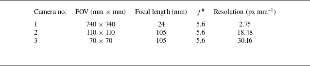

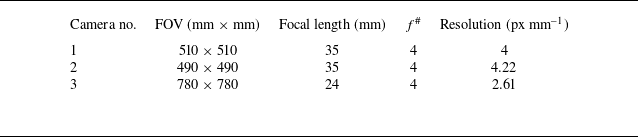
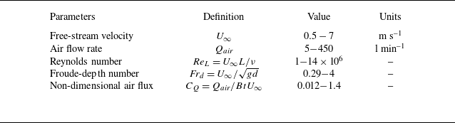
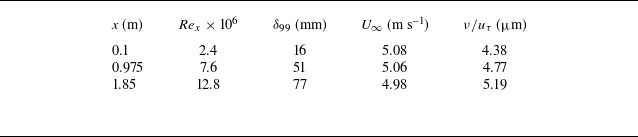


 Frd=1.24
 Qair=Qcrit
 x−y
 Qair=140
 x−y
 Qair=30

 Qair=10
 Qair=70
 Qair=140
 U∞=2
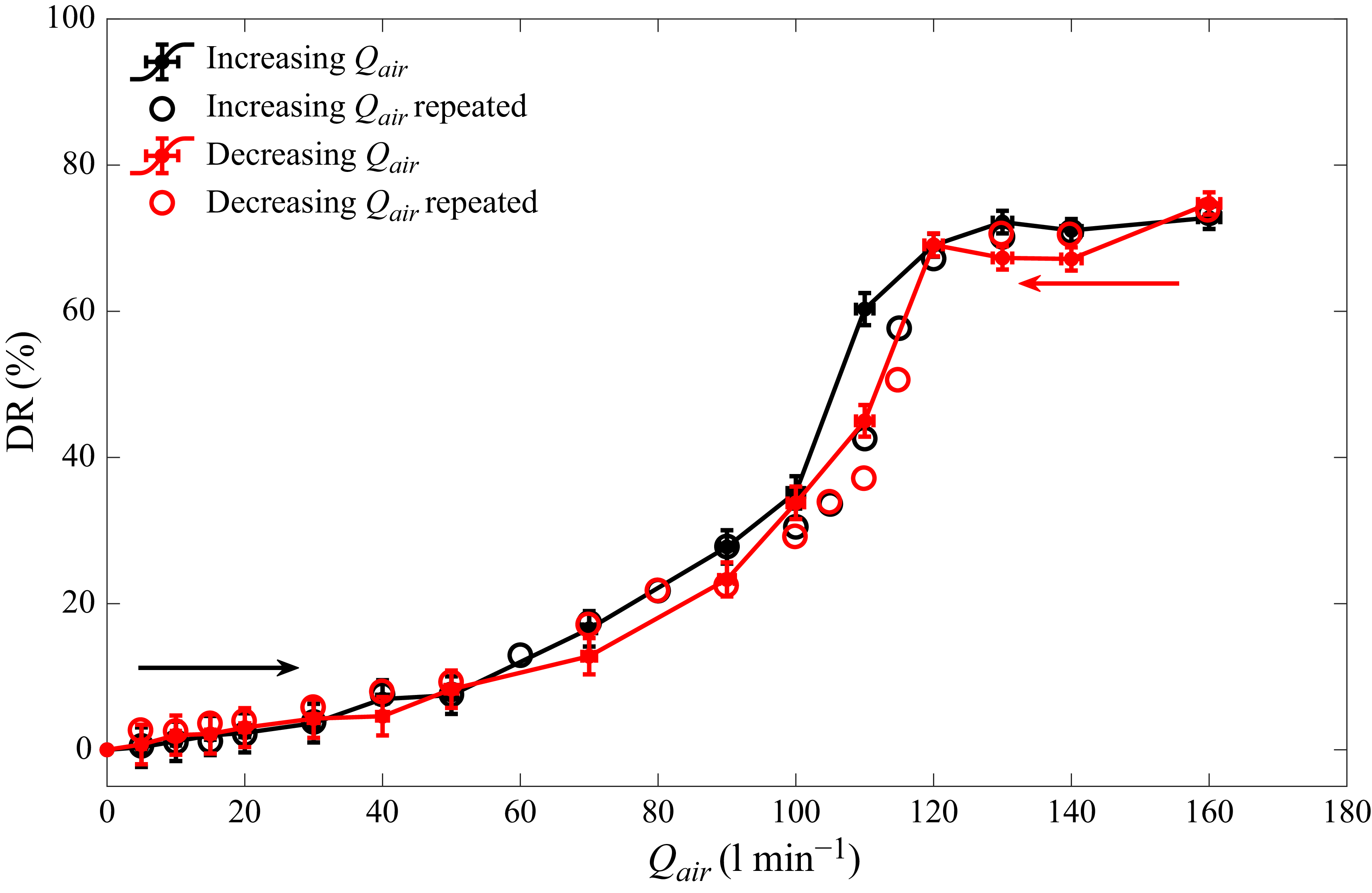
 U∞=3
 Frd=1.75
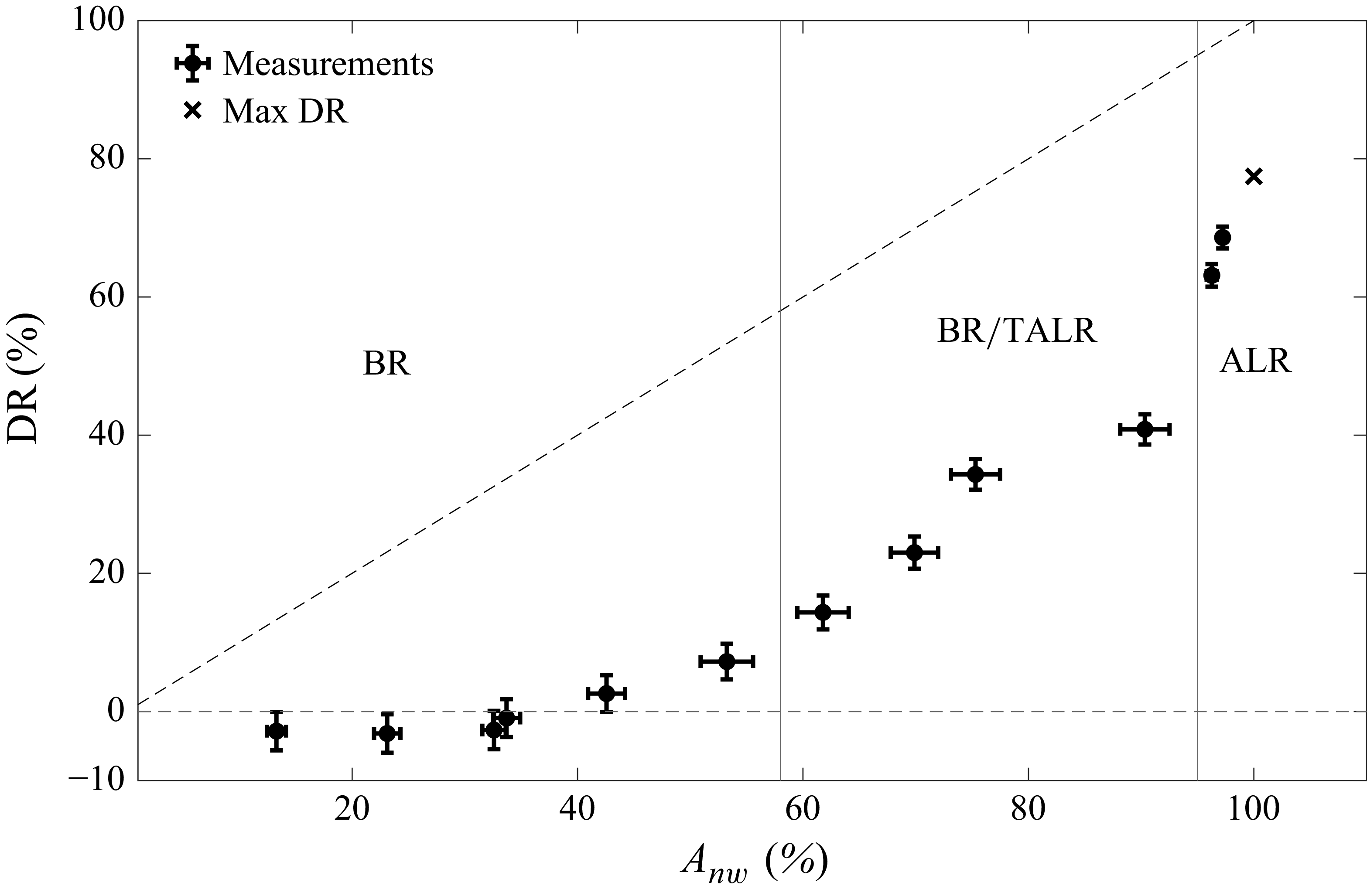
 U∞=2
 Frd=1.24
 DR=Anw

 U∞

 x−z
 U∞=5
 U∞=2
 Qair
 U∞

 U∞=2
 U∞=3.5
 db
 Qair=5
 40
 U∞=2
 U∞

 Qair=10
 U∞

 DR=40%

 x−z
 x−y
 DR≈40%
 U∞
 U∞=2
 Qair=80
 U∞=3.5
 Qair=130
 U∞=5
 Qair=200

 U∞=2
 tair
 tinj

 tinj
 θ
 U∞
 Qcrit
 tair
 Qair
 U∞
 Qair>Qcrit

 Qair=Qcrit
 Qair>Qcrit
 U∞
 U∞

 U∞
 Frd=1.24

 U∞=0.47
 Qair=20
 Frd=0.28
 U∞=0.57
 Qair=40
 Frd=0.33
 U∞=0.67
 Qair=40
 Frd=0.39
 U∞=0.93
 Qair=40
 Frd=0.54
 U∞=1.26
 Qair=60
 Frd=0.73
 Frd

 qtrans
 qcrit
 qair=Qair/B
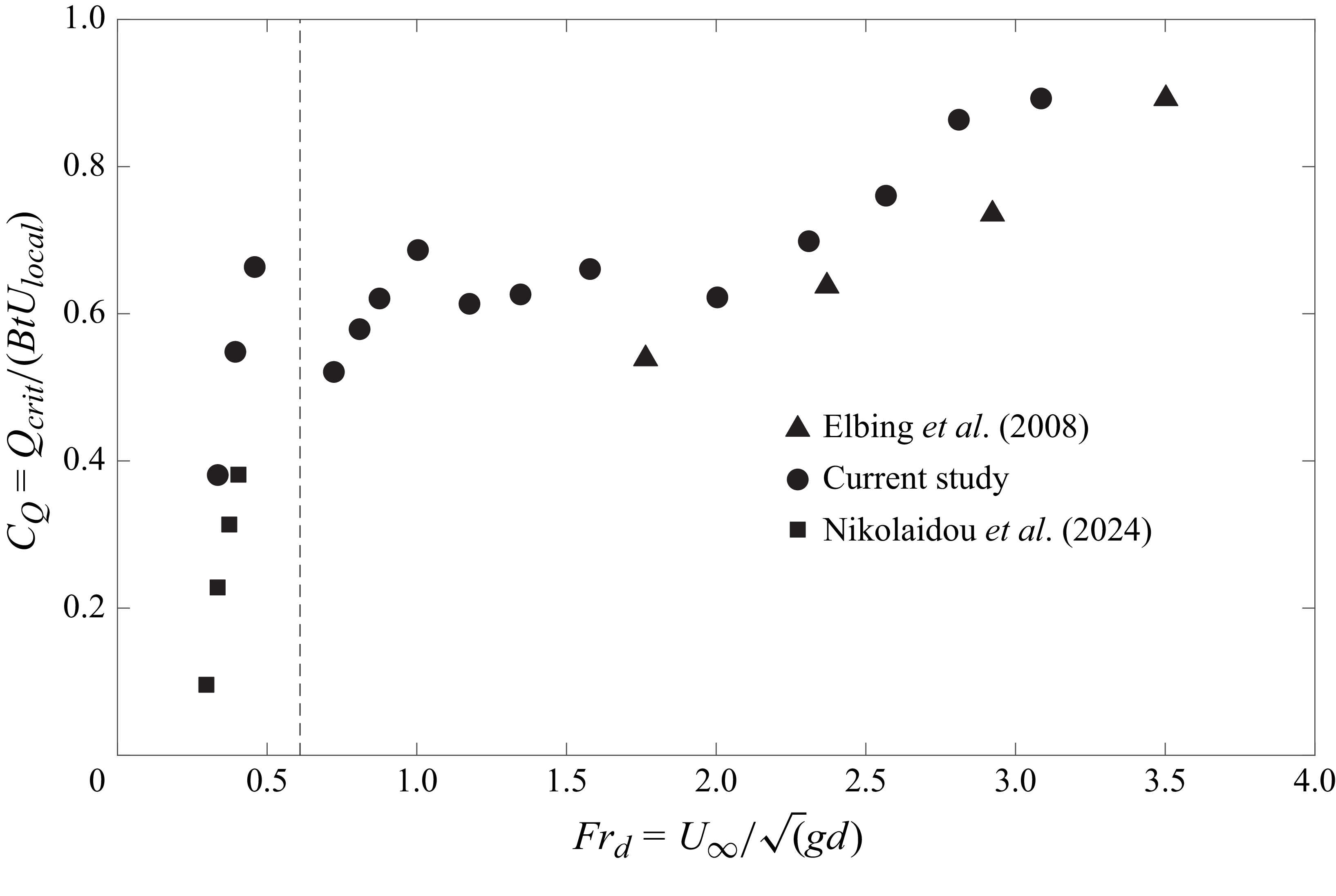
 Ulocal

 U∞=2.5
 U∞=3
 U∞=3.5
 U∞=5.5

 db
 U∞=3.5
 U∞=5

 Open access

