


…extreme heat is now the leading weather-related killer in America. Rising temperatures pose an imminent threat to millions of American workers exposed to the elements… (Joe Biden, September 2021)
High heat can be a big problem for the nation’s workers, not just farmworkers and construction workers, but delivery workers, utility workers, landscaping workers, and warehouse workers. (Steven Greenhouse, Nieman Reports, January 2023)
I. Introduction
High temperatures induced by climate change pose significant health risks to workers, especially those working in environments without climate controls (e.g., Luber and McGeehin (Reference Luber and McGeehin2008), Mora et al. (Reference Mora, Dousset, Caldwell, Powell, Geronimo, Bielecki, Counsell, Dietrich, Johnston, Louis, Lucas, McKenzie, Shea, Tseng, Giambelluca, Leon, Hawkins and Trauernicht2017)). For instance, Park, Pankratz, and Behrer (Reference Park, Pankratz and Behrer2021) estimate that high temperatures caused approximately 360,000 worker injuries in California from 2001 to 2018.Footnote 1 , Footnote 2 Notably, such temperature threats can affect a variety of economic outcomes; existing studies have highlighted the negative impact on aggregated output and income (e.g., Dell, Jones, and Olken (Reference Dell, Jones and Olken2009), Burke, Hsiang, and Miguel (Reference Burke, Hsiang and Miguel2015), and Behrer and Park (Reference Behrer and Park2017)). These findings are further corroborated by micro-level evidence demonstrating that extreme heat reduces individuals’ productivity by impairing physical and cognitive abilities (e.g., LoPalo (Reference LoPalo2023)).
Despite extensive research on heat risk and economic activity, three gaps remain. First, while climate change brings numerous challenges, less is known about how firms adapt to these risks (Fankhauser (Reference Fankhauser2017)). Understanding firms’ adaptation strategies is essential for guiding the business community’s response to a warmer climate. Second, existing evidence on the impact of heat risk on corporate performance is limited and mixed. For example, Addoum, Ng, and Ortiz-Bobea (Reference Addoum, Ng and Ortiz-Bobea2020) find no evidence that high temperatures affect corporate sales or labor productivity. In contrast, Pankratz and Schiller (Reference Pankratz and Schiller2024) and Custodio et al. (Reference Custodio, Ferreira, Garcia-Appendini and Lam2026) find that high temperatures reduce firm performance along supply chains. Addoum, Ng, and Ortiz-Bobea (Reference Addoum, Ng and Ortiz-Bobea2023) further document bidirectional effects of temperature on sales, with some firms experiencing losses and others benefiting. Third, although existing studies frequently cite labor productivity as an important channel, direct firm-level evidence examining this channel is scarce. For instance, Addoum et al. (Reference Addoum, Ng and Ortiz-Bobea2023) find strong support for a consumer demand channel but limited evidence for a labor productivity channel.
This article bridges these gaps in three steps. First, I introduce a novel method to quantify a labor channel of corporate exposure to climate risk, based on firms’ reliance on workers exposed to high temperatures while performing job duties. Second, through this channel, I examine firms’ adaptation to heat risk through capital deepening and automation. My reasoning is that high temperatures reduce the efficiency of workers relative to capital assets, such as algorithms, computers, machines, robots, and sensors, as production inputs. Consequently, firms may use more automated capital assets and less labor in production, leading to more capital-intensive production functions. Supporting this hypothesis, I find that high-exposure firms, defined as firms with labor exposure at the 75th percentile,Footnote 3 increase capital–labor ratios by 1.6%, increase capital expenditures and R&D expenses by 3.8%, invest 27.6% more in robotics-related human capital, and are 4.4% more likely to file automation patents after heat shocks. Third, I provide direct firm-level evidence that unexpected high temperatures reduce labor productivity, with high-exposure firms experiencing a 1.9% decline following heat shocks.
Capital deepening can serve as an adaptation strategy because it allows firms to reduce reliance on workers whose productivity is exposed to high temperatures. Automated capital assets can perform tasks that would otherwise require heat-exposed labor, thereby limiting operational disruptions when extreme heat reduces worker efficiency. Unlike some adaptation strategies, such as relocation or supply chain restructuring, automation can directly alter the input mix within firms’ existing production processes. Therefore, if heat risk makes labor less efficient relative to capital, firms have incentives to substitute capital for labor and adopt more capital-intensive production functions.
Crucial to my empirical investigations is the measurement of corporate exposure to climate risk from a labor perspective. To this end, I obtain data on occupations needed in each industry from the Occupational Employment and Wage Statistics (OEWS) and data on each occupation’s exposure to changing climates from the Occupational Information Network (O*NET) program. The exposure measure is based on how often a job requires working outdoors to fulfill duties.Footnote 4 I next construct an index of labor exposure at the 4-digit NAICS (NAICS4) level, calculated as the employment-weighted average of all occupations’ outdoor exposures. Based on this index, I create a rank variable of labor exposure to climate risk, ranging from 1 to 20, with 20 indicating the highest exposure. I further aggregate the exposure measure to the firm level using plant-level employment and industry classification data from Your Economy Time Series (YTS).
For temperature fluctuations, I obtain daily grid-level U.S. temperature data from the PRISM Climate Group. I construct a location- and time-specific measure of heat shocks for each county and year, defined as significant upward deviations from the county’s historical temperature distributions. I aggregate this measure to the firm level using firms’ geographic footprints across counties from YTS. By construction, the measure captures deviations from county- and time-specific historical temperature distributions and thus can be regarded as random draws from the distribution of temperatures within and across counties (Auffhammer et al. (Reference Auffhammer, Hsiang, Schlenker and Sobel2013), Dell, Jones, and Olken (Reference Dell, Jones and Olken2014)). Therefore, for any given firm, these shocks are plausibly exogenous.
To test the hypothesis of adaptation through capital deepening, I first examine firms’ capital utilization in production, a fundamental aspect of automation (e.g., Brozen (Reference Brozen1957), Acemoglu and Restrepo (Reference Acemoglu and Restrepo2019)), measured as the natural logarithm of total capital—property, plant, and equipment plus depreciation-adjusted R&D expenses. I also use the employment-scaled total capital as the dependent variable, that is, the capital–labor ratio, which captures the use of capital assets relative to labor in the production process. My analysis reveals no effect of heat shocks on the average firm’s capital utilization. However, for high-exposure firms, the effects are positive and statistically significant and hold after including firm, county-by-year, county-by-industry, and industry-by-year fixed effects. The findings also hold after accounting for exposure to non-heat climate events, are not driven by declines in crop yields, and persist under alternative measures of capital and heat shocks. The economic magnitude is significant. Following heat shocks, high-exposure firms increase their total capital utilization by 2.6% and capital–labor ratios by 1.6%. This evidence indicates that heat risk prompts exposed firms to adopt more capital-intensive production functions to ensure a resilient production system.
Additionally, I explore cross-sectional heterogeneity in firms’ capital deepening responses to heat challenges. I first find that heat shocks increase capital–labor ratios only among high-exposure firms operating in counties with significant projected long-term temperature increases. This evidence supports the prediction that firms respond primarily to heat threats that increasingly jeopardize their operations as climate change intensifies. Second, consistent with the notion that labor unions increase workers’ bargaining power and limit firms’ flexibility in workforce management, exposed firms increase capital intensity after heat shocks only in highly unionized industries. Third, the positive effects of heat shocks on capital–labor ratios arise only among high-exposure firms with low social ratings, suggesting that these firms may place less weight on employee welfare and are thus more likely to substitute capital for labor. Fourth, consistent with prior research showing that low-skilled tasks are easier to automate (Graetz and Michaels (Reference Graetz and Michaels2018)), heat shocks significantly affect capital–labor ratios only among exposed firms that predominantly employ low-skilled workers. Fifth, capital deepening after heat shocks occurs primarily among less complex exposed firms, as they are more agile in changing production inputs. Finally, the positive effects of heat shocks on capital utilization are concentrated among exposed firms with low financial constraints.
Moreover, to better understand how firms shift toward capital-intensive production functions, I examine their investments in physical capital assets and automation-related human capital. My analysis reveals that high-exposure firms increase capital expenditures and R&D expenses by 3.8% and post 27.6% more robotics-related jobs following heat shocks. Furthermore, I investigate firms’ innovation in automation-related technologies as part of the automation process. Using the classification of automation-related patents from Mann and Püttmann (Reference Mann and Püttmann2023), I find that the probability of filing at least one automation patent within 3 years after heat shocks increases by 4.4% for high-exposure firms.
As additional evidence, I examine firms’ disclosures of automation-related initiatives in 10-K filings. I find that heat-exposed firms discuss automation more frequently after heat shocks, particularly in contexts related to adaptation and risk mitigation. This evidence further supports the interpretation that firms use automation as an adaptation strategy to address heat-related challenges. Taken together, the findings on production functions, capital expenditures and R&D expenses, robotics-related human capital, automation technology, and automation disclosures provide consistent evidence that firms resort to automation to address escalating labor risks associated with high temperatures.
I further study labor productivity as one possible mechanism underlying firms’ automation responses. If heat risk reduces the efficiency of exposed workers, high-exposure firms should experience larger productivity losses following heat shocks, creating incentives to substitute capital for labor. Consistent with Addoum et al. (Reference Addoum, Ng and Ortiz-Bobea2020), the population average effect of high temperatures on labor productivity is zero. However, firms with substantial heat exposure through the labor channel experience significant reductions in labor productivity following heat shocks. The findings remain robust after including an extensive set of fixed effects that control for firm-, county-, and industry-level heterogeneity. The results also hold after accounting for non-heat climate events and are not driven by consumer demand or declines in crop yields. The results further hold under alternative measures of heat shocks and in plant-level and segment-level analyses. The effects are economically significant as well: high-exposure firms experience a 1.9% decline in labor productivity after heat shocks. This evidence suggests that extreme heat reduces the productivity of exposed workers and, consequently, affects the subset of firms that rely on these workers for production and operating activities.
Finally, I turn to whether capital deepening mitigates the adverse effects of heat risk and whether investors value firms’ adaptation efforts. If capital deepening helps firms address heat-related production disruptions, firms with more capital-intensive production functions should be less adversely affected by unexpected high temperatures. Consistent with this prediction, I find that the negative effects of heat shocks on labor productivity appear only among firms with below-median capital–labor ratios, while firms with above-median ratios do not experience significant declines, indicating greater operational resilience. I further find that heat shocks reduce the stock returns of exposed firms, but the effect is significantly weaker for firms with higher capital–labor ratios. These findings suggest that capital deepening can serve as an effective adaptation strategy and that investors appear to value firms’ adaptation capacity.
II. Related Literature
A. Adaptation to Climate Change
This article relates to research on adaptation strategies adopted by economic agents to mitigate climate risks (e.g., Behrer and Park (Reference Behrer and Park2017), Fankhauser (Reference Fankhauser2017), and Lai et al. (Reference Lai, Qiu, Tang, Xi and Zhang2023)). Despite extensive discussion in other fields, research on adaptation behavior in the business sector remains limited, with a few exceptions. Somanathan et al. (Reference Somanathan, Somanathan, Sudarshan and Tewari2021) show that climate controls can eliminate plant-level productivity declines caused by high heat in India, while Heyes and Saberian (Reference Heyes and Saberian2019) document limited effects. However, these studies focus on indoor environments where climate controls, such as air conditioning, can be implemented, rather than outdoor settings, where doing so is costly or impossible (Dillender (Reference Dillender2021)). In addition, Pankratz and Schiller (Reference Pankratz and Schiller2024) show that firms mitigate heat risk through supply chain management, while Acharya, Bhardwaj, and Tomunen (Reference Acharya, Bhardwaj and Tomunen2024) document workforce reallocation as a response to heat. In contrast, I show that firms increase capital deepening and automation as adaptation strategies to mitigate heat risk, thereby reducing labor productivity losses and increasing firm value. Consequently, this article responds to the call for more research on adaptation to climate change (Fankhauser (Reference Fankhauser2017)).
Xiao (Reference Xiao2023) shows that firms increase announcements of automation-related investments following high temperatures. This study differs by i) focusing exclusively on outdoor heat and excluding production-generated heat unrelated to climate change; ii) using comprehensive grid-level daily temperature data to identify abnormal heat based on past temperature distributions; iii) examining firms’ adaptation through changes in capital–labor intensity, capital expenditures and R&D investments, robotics-related human capital, automation technologies, and automation disclosures in 10-K filings; and iv) studying the implications of these adaptations for firm resilience and market value.
B. Climate Change, Heat Risk, and Labor Productivity
This article also contributes to the growing climate finance literature by deepening our understanding of how climate change, particularly high temperatures, affects firms’ production activities. It develops a novel measure of firms’ climate exposure from a labor perspective, enabling firm- and plant-level analyses of how heat risk affects labor productivity, an area in which existing evidence remains mixed. For example, Addoum et al. (Reference Addoum, Ng and Ortiz-Bobea2020) find no evidence that high temperatures affect the sales or labor productivity of U.S. firms and plants. Other studies show that increased temperatures reduce firms’ operating performance (Pankratz, Bauer, and Derwall (Reference Pankratz, Bauer and Derwall2023)) and that these effects transmit along supply chains (Pankratz and Schiller (Reference Pankratz and Schiller2024), Custodio et al. (Reference Custodio, Ferreira, Garcia-Appendini and Lam2026)). In addition, while existing studies frequently cite labor productivity as an important channel, direct firm-level evidence on this channel is scarce. My study provides evidence that heat risk reduces labor productivity in U.S. firms and plants, but only among those with significant temperature exposure through the labor channel. This evidence supports reduced labor efficiency relative to capital as one potential mechanism underlying firms’ capital deepening and related automation investments in response to heat challenges.
III. Conceptual Framework
A. Climate Change, Workplace Safety, and Labor Efficiency in Production
Heat exposure can cause a variety of heat-related illnesses, such as heat cramps and heat stroke (Luber and McGeehin (Reference Luber and McGeehin2008), Mora et al. (Reference Mora, Dousset, Caldwell, Powell, Geronimo, Bielecki, Counsell, Dietrich, Johnston, Louis, Lucas, McKenzie, Shea, Tseng, Giambelluca, Leon, Hawkins and Trauernicht2017)). As global warming intensifies, rising temperatures will increasingly threaten workers’ health (Dillender (Reference Dillender2021), Park et al. (Reference Park, Pankratz and Behrer2021)), impairing their physical and cognitive abilities (Heyes and Saberian (Reference Heyes and Saberian2019), Park et al. (Reference Park, Goodman, Hurwitz and Smith2020)), and ultimately their productivity (Chen and Yang (Reference Chen and Yang2019), LoPalo (Reference LoPalo2023)). Even the world’s wealthiest economy is subject to material heat-related productivity losses (Deryugina and Hsiang (Reference Deryugina and Hsiang2014), Burke et al. (Reference Burke, Hsiang and Miguel2015), and Behrer and Park (Reference Behrer and Park2017)).
Studies also show that exposed workers reduce working time during hot days, implying a contraction in labor supply (Graff Zivin and Neidell (Reference Graff Zivin and Neidell2014), Dillender (Reference Dillender2021), Somanathan et al. (Reference Somanathan, Somanathan, Sudarshan and Tewari2021)). To attract and retain workers, firms must offer either more pecuniary compensation or non-pecuniary benefits, such as cooling services, to alleviate heat risks. Failure to do so would expose firms to significant reputational damage and litigation risks if workers suffer injuries or fatalities (Ortiz-Molina, Xiao, and Zheng (Reference Ortiz-Molina, Xiao and Zheng2026)).
These findings identify four channels through which heat risk may reduce the efficiency of labor as a production input: i) lower productivity at work, ii) reduced labor supply, iii) higher non-wage labor costs, and iv) greater reputational and litigation risks. While the neoclassical economic framework posits that labor inputs are fully flexible and have little impact on firms’ operations, the reality is different; firms face frictions that impede their labor adjustments. Labor unions, for instance, often intervene in firms’ wage and firing decisions. Regulations on labor protection further limit firms’ discretion in adjusting wages and workforce. These rigidities increase firms’ operating leverages and decrease their values. Therefore, high temperatures reduce labor efficiency in production and push up firms’ production costs per unit of output.
B. Adaptation to Climate Change Through Capital Deepening and Automation
Heat-induced reductions in labor efficiency create incentives for firms to adjust production processes and build more resilient operations. Moreover, salient heat events lead managers to update their beliefs about climate change and pay greater attention to climate risks (e.g., Sisco, Bosetti, and Weber (Reference Sisco, Bosetti and Weber2017), Choi, Gao, and Jiang (Reference Choi, Gao and Jiang2020)), further motivating adaptation. This raises the question of how firms adjust their production strategies in response.
Automation offers one potential solution, as firms across industries have developed equipment that can operate in extreme conditions. For instance, manufacturers use Computer Numerical Control (CNC) machinery and robotic arms, while chemical and pharmaceutical firms use robots to transfer and process hazardous materials. By delegating tasks to resilient automated equipment, firms can increase productivity while protecting workers in challenging conditions (e.g., Bellingham and Rajan (Reference Bellingham and Rajan2007), Gihleb et al. (Reference Gihleb, Giuntella, Stella and Wang2022)). Similarly, firms can deploy automation assets to address heat-related threats to production. These assets need not be “green” or climate-specific; as long as they can replace heat-exposed workers and operate effectively under high temperatures, firms can use them as substitutes for labor.Footnote 5
Notably, the feasibility of adaptation through automation rests on three assumptions. The first is that extreme heat impacts the performance of capital assets less than that of workers.Footnote 6 The second is that automation serves as a key strategy for firms to mitigate temperature challenges.Footnote 7 The third is that the costs of using capital assets in production are lower than those of using exposed labor.Footnote 8 Crucially, if any of the assumptions is violated, I should not find significant effects of heat risk on automation. Put differently, if capital assets prove unreliable or too costly in hot conditions, or if firms predominantly use strategies other than automation to address heat risks, the effects on automation should not be observable in the data.
In summary, heat risk reduces labor efficiency relative to capital in production. Firms can address this challenge by shifting toward more capital-intensive production functions. As extreme heat becomes more frequent and severe, heat-exposed firms are expected to further enhance automation.Footnote 9
IV. Data, Measures, and Sample
A. Firms
I collect data on public firms and their balance sheet information (annual and quarterly) from the Compustat/CRSP Merged database. I exclude firms from financial, utility, public administration, and unclassified industries. Firms headquartered outside of the U.S. are also excluded. Information on firms’ historical headquarters state, county, and industry classifications is compiled from the “Augmented 10-X Header Data” provided by Bill McDonald and “Company Headquarters” provided by Joshua A. Lee.
B. Plants
Data on the distribution of a firm’s plants across locations come from the YTS database, provided by the Business Dynamics Research Consortium (BDRC) at the University of Wisconsin. YTS provides detailed establishment-level information, including plant location (e.g., county and ZIP code), industry classification (e.g., NAICS code), place type (e.g., headquarters, subsidiary, or independent), employment, sales, and parent company identifiers. The data set is constructed from Data Axle (formerly Infogroup) business records and links establishments over time using unique identifiers (American Business Identifiers, ABIs) to create a longitudinal panel.Footnote 10 The data are available annually from 1997 and have been widely used in academic research and policy analysis, including Ghent (Reference Ghent2021), Campello et al. (Reference Campello, Cortes, d’Almeida and Kankanhalli2022), Flynn and Ghent (Reference Flynn and Ghent2022), Coyne and Johnson (Reference Coyne and Johnson2023), and Arefeva et al. (Reference Arefeva, Davis, Ghent and Park2025).Footnote 11
In this study, YTS is used to identify the geographic locations, industry classifications, and employment levels of firms’ plants. Because the underlying Data Axle records rely on verified business addresses and the analysis uses county-level geographic information rather than finer spatial measures, the location information is generally reliable. Data Axle assigns industry classifications based on Yellow Pages headings and verifies businesses through telephone interviews to confirm their accuracy, and YTS further refines these classifications. In addition, plant employment is used primarily as a size weight when aggregating county-level heat risk to the firm level; therefore, moderate measurement error in employment is unlikely to materially affect the estimation results.Footnote 12
C. Labor Exposure to Climate Risk
To quantify corporate exposure to climate risk through a labor channel, I first obtain data on occupations from the OEWS. This data includes occupations needed in each industry and the number of employees working in each occupation. Then, I collect data on each occupation’s current and historical exposures to climate conditions from the Department of Labor’s Occupational Information Network (O*NET) program. This study uses the survey that focuses on the working context of “Outdoors, Exposed to Weather.” Specifically, O*NET gives each occupation a score between 1 and 5 based on the following question—“How often does this job require working outdoors, exposed to all weather conditions?” A higher score indicates greater exposure to climate conditions while performing job duties.Footnote 13
Using these two data sets, I construct a labor exposure to climate risk index as follows:

where
$ i $
 denotes industry,
$ o $
 denotes occupation, and
$ t $
 denotes year.
$ {O}_{i,t} $
 is the total number of occupations industry
$ i $
 has in year
$ t $
 .
$ {Score}_{o,t} $
 is the occupational score of outdoor activity.
$ {Emp}_{i,o,t} $
 is the number of employees working in occupation
$ o $
 in industry
$ i $
 in year
$ t $
 .
$ {Emp}_{i,t} $
 is the total number of employees in industry
$ i $
 in year
$ t $
 . This index is therefore the employment-weighted average outdoor exposure across occupations within a NAICS4 industry. I then create a rank variable
$ {Labor\ Exposure}_{i,t} $
 , ranging from 1 to 20, with 20 indicating the highest exposure.
Figures IB.1, IB.2, and IB.3 and Table IB.2 in the Supplementary Material present distributions of the exposure measure across sectors, labor skills, and counties. A key takeaway is that significant variations exist in workers’ climate exposures within and across sectors, skill levels, and counties, indicating that this measure does not simply capture sector-, skill-, or county-specific heterogeneities. The widespread presence of high-exposure occupations and industries suggests that high temperatures have a comprehensive impact on the entire economy. Further, in Figures IB.4, IB.5, IB.6, IB.7, and IB.8 in the Supplementary Material, I validate the labor exposure measure by showing that managers of high-exposure firms discuss more climate issues in earnings conference calls and 10-K filings, suggesting that dependence on outdoor workers exposes firms to significant climate risks. Additionally, this labor channel cannot be fully explained by other measures of climate exposure developed in the literature or by Trucost Climate Analytics. This evidence highlights the importance of, and lays the foundation for, studying corporate exposure to climate change and adaptation through a labor channel.
YTS assigns each plant an industry classification based on its business operations. I aggregate labor exposure to the firm level using plant-level employment and NAICS4 codes from YTS as follows:

where
$ f $
 denotes firm,
$ i $
 denotes NAICS4 industry, and
$ t $
 denotes year.
$ {I}_{i,t} $
 is the number of industries in which firm
$ {f}^{\prime }s $
 plants operate.
$ {Emp}_{f,i,t} $
 is firm
$ {f}^{\prime }s $
 employment in industry
$ i $
 .
$ {Emp}_{f,t} $
 is firm
$ {f}^{\prime }s $
 total employment.
$ Labor\;{Exposure}_{i,t} $
 is the industry-level labor exposure measure in equation (1). The firm-level labor exposure is therefore the employment-weighted average of industry-level exposure across a firm’s NAICS4 industries. I also construct a labor skill measure based on O*NET job zones using the same method.
D. Heat Shocks
I obtain data on daily temperatures and precipitation for 1981–2022 from the PRISM Climate Group. The data covers each of 481,631 16-square-kilometer (i.e., 4
$ \times $
 4 km) grids for the continental United States and includes daily mean, minimum, and maximum temperatures, as well as precipitation levels. I aggregate the grid-level information to the county level.Footnote
14
This article examines how unexpected high temperatures affect firms’ labor productivity and adaptation strategies conditional on their labor exposures. To do so, I construct a measure of heat shocks, conceptually similar to the abnormal heat measure in Addoum et al. (Reference Addoum, Ng and Ortiz-Bobea2020) and the abnormal snow measure in Brown, Gustafson, and Ivanov (Reference Brown, Gustafson and Ivanov2021). This approach improves upon the use of temperature levels by accounting for firms’ dynamic adaptations to local climate conditions, such as adjustments in production processes and locations.Footnote 15
First, I calculate the 90th percentile of historical temperature distributions for each county on a monthly basis, using temperature data from 1981 up to the previous year, with a maximum of 30 years. Second, for each day within a given county and month, I compare the realized daily maximum temperature with the estimated 90th percentile to identify abnormally hot days, that is, Realized Temperatures
$ \ge $
 90th Percentile. Third, since the subsequent empirical analyses are conducted at the yearly level, I aggregate the number of hot days during summer months each year to create a measure that captures significant upward shifts in temperature distributions compared to historical data.Footnote
16 Specifically,

where
$ c $
 denotes county and
$ t $
 denotes year.
$ Realized\;{Temperatures}_{c,t} $
 is daily maximum temperatures in county
$ c $
 and year
$ t $
 .
$ 90\mathrm{th}\hskip0.32em {\mathrm{Percentile}}_{c,t} $
 is the estimated 90th percentile of county
$ c $
 ’s past temperatures.
$ No.\hskip0.32em Hot\hskip0.32em Days $
 is the number of hot days in summer in county
$ c $
 and year
$ t $
 , based on “
$ Realized\hskip0.42em {Temperatures}_{c,t}\ge 90\mathrm{th}\hskip0.32em {\mathrm{Percentile}}_{c,t} $
 .”
$ T $
 is the threshold to identify abnormally hot summers after adjusting for seasonality and location.
This method identifies hot days in a relative sense by comparing current temperatures to historical temperatures for the same county and month. For each specific county, if there are no changes in temperature distributions from the past to the current year, one would anticipate approximately 10 days (
$ T=10 $
 ) to be flagged as hot.Footnote
17 If a summer experiences more than 10 hot days (
$ T>10 $
 ), it implies an upward shift in temperature distributions. Put differently, any additional hot days beyond the expected 10 signify unexpected heat risk.Footnote
18 To capture a significant upward shift and, consequently, an unlikely overlooked heat shock, I set the threshold at
$ T=15 $
 , a 50% increase relative to the benchmark 10 days, which identifies the top-quartile cases with severe relative heat shocks.Footnote
19
Figure 1 presents the average number of relative hot days for each county in the continental United States across years. The occurrence of relative hot days is not concentrated in any specific county but instead occurs in different counties over time. Therefore, for any given firm, heat shocks are plausibly exogenous and randomly distributed across its operating locations, making it difficult for firms to take precautionary actions ex ante.Footnote 20
Figure 1 presents the number of summer days with relative heat shocks (equation (3)) for each county in the continental United States in the years 2000, 2006, 2009, 2012, 2015, and 2018.

FIGURE 1 Long description
A six-panel series of choropleth maps labeled Graph A through Graph F. Each map uses a color gradient from pale yellow (0 to 5 days) to dark burgundy (30 plus days) to represent the number of summer days with relative heat shocks.
* Graph A. Year 2000: High concentrations are visible in the Central and Southeast regions, particularly in the Deep South.
* Graph B. Year 2006: Intense heat shock clusters appear in the Southwest, the Southern Plains, and the Southeast.
* Graph C. Year 2009: The highest frequency is concentrated almost exclusively along the Gulf Coast and the Southern tip of Texas.
* Graph D. Year 2012: Shows the most widespread high-intensity heat shocks, covering nearly the entire Midwest, Central Plains, and Ohio River Valley.
* Graph E. Year 2015: Heat shocks are most prominent in the Northwest and along the Southern border with Mexico.
* Graph F. Year 2018: Moderate to high concentrations are scattered across the Southwest, the Southern Plains, and parts of the Southeast.
Each map includes a legend in the bottom-left corner with six intervals: 0-5, 6-10, 11-15, 16-20, 21-25, 26-30, and 30 plus.
I aggregate county-level heat shocks to the firm level using plant-level employment and location data from YTS as follows:


where
$ f $
 denotes firm,
$ c $
 denotes county, and
$ t $
 denotes year.
$ {C}_{f,t} $
 is the total number of counties in which firm
$ {f}^{\prime }s $
 plants operate.
$ {Emp}_{f,c,t} $
 is firm
$ {f}^{\prime }s $
 employment in county
$ c $
 and year
$ t $
 .
$ {Emp}_{f,t} $
 is
$ {f}^{\prime }s $
 total employment in year
$ t $
 .
$ No. Hot\;{Days}_{f,t} $
 is the employment-weighted average of firm
$ {f}^{\prime }s $
 exposure to heat shocks across counties in year
$ t $
 . For consistency, I still set
$ T=15 $
 to define heat shocks at the firm level.
Additionally, I construct a county-level measure of cumulative medium-term heat shocks, 1(Realized
$ \gg $
 expected)(M), following equations (3) and (4), with two modifications, in order to capture the gradual intensification of unexpected heat risk over time that may trigger adaptation responses. First, I calculate the total number of relatively hot days in summers over the period from
$ t-3 $
 to
$ t $
 . Second, I set the threshold at
$ T=45 $
 , relative to the benchmark of 40, to define medium-term heat shocks, that is,
$ No. Hot\;{Days}_{t-3,t}\ge 45 $
 .Footnote
21 This threshold corresponds to approximately a 12.5% increase relative to historical temperature distributions, or at least one significant short-term heat shock over the period, that is,
$ 45=15+10+10+10 $
 .
E. Additional Data
Temperature Projections. County-level long-term temperature projections are sourced from the Centers for Disease Control and Prevention (CDC). The data give projected differences in extremely hot days (90°F/32.2°C) between the time period selected (2016–2045) and the referent period (1976–2005).
Patents. Data on firms’ patenting activities are from Kogan et al. (Reference Kogan, Papanikolaou, Seru and Stoffman2017). It includes the applicant’s PERMNO number, filing year, grant year, and the estimated patent value. Data on the classification of automation-related patents are from Mann and Püttmann (Reference Mann and Püttmann2023), which applies a machine learning algorithm to all U.S. patents granted from 1976 to 2014 to identify automation-related patents, that is, patents used to develop a device that carries out a process independently of human intervention. The device can be a physical machine, a combination of machines, an algorithm, or a computer program.
F. Sample and Summary Statistics
The final empirical sample spans the period 1999–2019.Footnote 22 Table 1 reports summary statistics for key variables used in empirical analyses. The average use of capital and capital per employee are 4.914 and 4.364, respectively. The mean and median of firm labor productivity are 4.144 and 4.100, with a standard deviation of 0.835. Meanwhile, 18.6% of firms are exposed to short-term temperature shocks, while 27.4% are exposed to medium-term ones. The average rank of labor exposure to climate risk is 8 at the NAICS4 industry level.

TABLE 1 Long description
The table contains 24 rows of variables and 6 columns of statistics: Number of Observations, Mean, P 5, Median, P 95, and Standard Deviation.
Key data points include:
* Log Capital: 60,384 observations, mean 4.914, median 4.827.
* Capital investment rate: 57,179 observations, mean minus 2.627, median minus 2.565.
* Robotics-related human capital: 11,322 observations, mean 0.087, median 0.000.
* Automation technology: 42,443 observations, mean 0.242, median 0.000.
* Automation count: 49,117 observations, mean 224, median 100, P 95 of 1,300.
* Automation share: 49,117 observations, mean 885, median 201, P 95 of 5,338.
* Log Sale over Emp: 60,129 observations, mean 4.144, median 4.100.
* O I B D P over Emp: 56,851 observations, mean 15.115, median 6.071, standard deviation 93.347.
* Return percentage: 55,839 observations, mean 8.088, median 3.674, standard deviation 45.302.
* Temperature variation: 61,478 observations, mean 6.323, median 5.909.
* Labor exposure: 61,478 observations, mean 7.833, median 6.000, P 95 of 18.000.
* Size: 61,478 observations, mean 6.244, median 6.160.
* Book leverage: 61,217 observations, mean 0.232, median 0.199.
* Log 1 plus number of patents: 42,443 observations, mean 2.001, median 0.
* C A P M beta: 53,259 observations, mean 1.049, median 1.016.
V. Adaptation Through Capital Deepening and Automation
Section III discusses the rationale underlying firms’ adaptation to heat risk through automating tasks performed by heat-exposed workers. Because automation requires greater use of capital and therefore raises capital intensity in production (e.g., Brozen (Reference Brozen1957), Karabarbounis and Neiman (Reference Karabarbounis and Neiman2014), Acemoglu and Restrepo (Reference Acemoglu and Restrepo2019), Acemoglu and Restrepo (Reference Acemoglu and Restrepo2020)), I examine firms’ use of capital assets—such as algorithms, computers, equipment, machines, robots, and sensors—as well as related investments, including capital expenditures, R&D, the acquisition of robotics-related human capital, and the development of automation-related technologies. I also examine firms’ disclosures of automation initiatives following heat shocks.
A. Empirical Methodology
Adaptation through automation can be costly, time-consuming, and challenging. For example, dismissing workers displaced by automation can be onerous, particularly in the presence of labor unions and regulations. Adopting new capital assets requires substantial financial resources and the hiring and training of skilled workers capable of operating them. Consequently, firms might not resort to automation immediately or fully after a one-time short-term heat shock. Instead, they adjust production inputs gradually over time as they perceive persistent medium- or long-term temperature risks. To capture this gradual adjustment, I examine firms’ automation responses to medium-term heat shocks using the following empirical specification.

where
$ f $
 denotes firm,
$ c $
 denotes headquarters county,
$ i $
 denotes 2-digit NAICS (NAICS2) industry code, and
$ t $
 denotes year.
$ Y $
 is the dependent variable measuring a firm’s automation progress.
$ 1\left( Realized\gg Expected\right)(M) $
 is a dummy indicating firm
$ {f}^{\prime }s $
 exposure to medium-term heat shocks.
$ Labor\ Exposure $
 measures firm
$ f $
 ’s average exposure to climate risk through the labor channel, as defined in equations (1) and (2), over the period from
$ t-3 $
 to
$ t $
 .
$ \boldsymbol{X} $
 is a vector of controls including the logarithm of total assets (Size), market-to-book ratio (M/B), book leverage (Book leverage), cash holdings (Cash), and a dummy indicating whether a firm pays dividends (Dividend payer).
$ {\mu}_f $
 is firm fixed effects that control for firm-level time-invariant characteristics.
$ {\tau}_{c,t} $
 is county-by-year fixed effects that control for time-varying changes in county
$ c $
 .
$ {\theta}_{c,i} $
 is county-by-NAICS2 industry fixed effects that control for the importance of industry
$ i $
 in county
$ c $
 .
$ {\pi}_{i,t} $
 is NAICS2 industry-by-year fixed effects that control for time-varying growth trends of industry
$ i $
 .
B. Capital Utilization in Production
1. Main Results
Table 2 examines how firms adjust their use of capital in production following heat shocks. Columns 1–4 use the natural logarithm of total capital, Log(Capital), as the dependent variable. Total capital is defined as the sum of a firm’s property, plant, and equipment (PPENT) and its R&D stock. R&D stock is the sum of a firm’s past R&D expenses, assuming a 20% depreciation rate, capturing the accumulation of intangible research capital that supports automation.Footnote 23 Columns 5–8 use the natural logarithm of employment-scaled total capital, Log(Capital/Emp), as the dependent variable. This measure captures the capital–labor ratio, reflecting firms’ use of capital relative to labor in production. A higher ratio indicates a more capital-intensive production function and a higher degree of automation (Brozen (Reference Brozen1957)).

TABLE 2 Long description
The table is divided into two main sections based on the dependent variable: Log(Capital) times 100 for columns 1 through 4, and Log(Capital/Emp) times 100 for columns 5 through 8.
Key Independent Variables:
* 1 (Realized much greater than expected) (M): Coefficients range from -1.916 in column 3 to 0.604 in column 1. Significant negative effects are seen in columns 3, 6, 7, and 8.
* 1 (Realized much greater than expected) (M) times Labor exposure: Shows consistently positive and significant coefficients across all models where included, ranging from 0.227 to 0.371, all significant at the 1 percent or 5 percent level.
* Labor exposure: Coefficients are generally non-significant, except for a negative effect of -0.534 in column 8.
Fixed Effects and Controls:
* All models include Controls and Firm F E.
* State times year F E is included in columns 1, 2, 5, and 6.
* County times year F E is included in columns 3, 4, 7, and 8.
* County times N A I C S 2 F E and N A I C S 2 times year F E are included in columns 4 and 8.
* Adjusted R-squared values are high, ranging from 0.935 to 0.973.
Treatment Effects:
* At Labor exposure equals 15, effects are positive and significant across all models, ranging from 1.623 to 2.888.
* At Labor exposure equals 20, effects increase in magnitude and significance, ranging from 2.757 to 4.677.
In columns 1 and 5, the estimated coefficient on heat shocks, 1 (Realized
$ \gg $
 expected) (M), is positive but statistically insignificant, indicating that heat shocks do not affect capital utilization for the average firm. In columns 2, 3, 6, and 7, the coefficient on 1 (Realized
$ \gg $
 expected) (M) becomes negative and significant, suggesting that a hypothetical firm with zero exposure reduces capital utilization after heat shocks.Footnote
24
Importantly, the interaction term between heat shocks and labor exposure (1 (Realized
$ \gg $
 expected) (M)
$ \times $
 Labor exposure) is positive and statistically significant. The results are not driven by firm-level time-invariant or county-level time-varying characteristics, given the inclusion of firm and county-by-year fixed effects. In columns 4 and 8, after adding county-by-NAICS2 industry and NAICS2 industry-by-year fixed effects, the significance of 1 (Realized
$ \gg $
 expected) (M)
$ \times $
 Labor exposure remains. The economic magnitude is large. In column 4, the post-estimation test suggests that total capital utilization increases by 2.6% for firms with heat exposure at the 75th percentile and by 3.9% for firms with the highest exposure. In column 8, the capital–labor ratio increases by 1.6% for firms with heat exposure at the 75th percentile and by 2.8% for firms with the highest exposure. The economic effects for firms in each exposure category are reported in Table ID.1 in the Supplementary Material. Overall, these findings demonstrate that past heat shocks prompt exposed firms to enhance their capital utilization in production processes, as evidenced by a significant increase in total capital and capital–labor ratios.
2. Robustness Checks and Ruling Out Alternative Explanations
Section D of the Supplementary Material presents additional analyses to demonstrate the robustness of the capital utilization results in Table 2 and to rule out alternative explanations. I briefly discuss these results subsequently.
Measurement of Capital Excluding R&D Capital. In Table ID.2 in the Supplementary Material, I reconstruct the measures of total capital utilization and capital–labor ratios using PPENT only, excluding depreciation-adjusted R&D expenses. The results remain consistent.
Accounting for Temperature Levels. In Table ID.3 in the Supplementary Material, I reconstruct the measure of heat shocks by incorporating absolute temperature levels, that is, number of summer days above 30 °C from
$ t-3 $
 to
$ t $
 . The results hold, and the economic magnitudes are larger.
An Alternative Rolling Window to Define Heat Shocks. In Table ID.4 in the Supplementary Material, I use a 20-year rolling window, instead of a 30-year window, to estimate the 90th percentile threshold for measuring heat shocks. The results remain consistent, with larger economic magnitudes.
Heat Shocks in Firm Headquarters County. Table ID.5 in the Supplementary Material focuses on headquarters-county heat shocks, and the results are largely consistent.
Controlling for Other Climate Events. In Table ID.6 in the Supplementary Material, I repeat the analysis by controlling for other types of climate events. In Panel A, I control for cold temperature shocks and total precipitation, while in Panel B, I account for heat shocks occurring outside the summer season and all disasters reported by FEMA. I find no significant effects of these non-heat climate events on firms’ capital utilization in production. The effects of heat shocks on capital utilization remain robust, with similar economic magnitudes.
Sector Breakdowns and Excluding A Consumer Demand Channel. I exclude agricultural and consumer-oriented industries in Table ID.7 in the Supplementary Material and non-tradable industries in Table ID.8 in the Supplementary Material. The results continue to hold, with similar economic magnitudes, suggesting that the findings on heat-induced capital deepening are not driven by the consumer demand channel or by declines in crop yields.
Alternative Measures of Labor Exposure. Table ID.9 in the Supplementary Material repeats the analysis using the firm-level measure of labor exposure defined in equation (2), and Table ID.10 in the Supplementary Material reports robustness checks using a continuous measure of labor exposure instead of the rank-based measure. The results hold in both analyses.
3. Heterogeneity
I further explore cross-sectional heterogeneity in the effects of heat shocks on firms’ capital utilization in production to better understand the underlying economic mechanisms.
First, I examine the role of projected long-term temperature increases in firms’ operating locations. The capital response should be concentrated in locations with large projected temperature increases, where current heat shocks are more likely to signal persistent and worsening future heat risk. In these areas, firms have stronger incentives to reorganize production processes and invest in automated capital assets to improve operational resilience. By contrast, when projected temperature increases are limited, firms may view current heat shocks as less informative about future operating conditions and therefore have weaker incentives to adapt. To test this conjecture, I categorize firms into two groups based on whether projected temperature increases in their operating counties are above or below the sample median. I then examine the effects of heat shocks on capital utilization separately for each group. The analysis in columns 1 and 2 of Panel A of Table 3 shows that the interaction term between heat shocks and labor exposure is positive and statistically significant only for firms in counties with large projected temperature increases, whereas the estimate is insignificant for firms in counties with small projected increases.

TABLE 3 Long description
The table is divided into two main sections.
Panel A, titled Expected Heat Risk, Incentives, and Operating Constraints, contains 10 columns grouped by Temperature Projections, Labor Union, Social Ratings, Labor Skill, and Firm Complexity, each split into High H and Low L categories. The dependent variable is Log(Capital/Emp) times 100.
* For the variable 1(Realized >> expected) (M), the most significant negative coefficient is in Column 1 (High Temperature Projections) at -4.175.
* The interaction term 1 (Realized >> expected) (M) times Labor exposure shows positive significant coefficients in Column 1 (0.470), Column 3 (0.315), Column 6 (0.583), Column 8 (0.288), and Column 10 (0.315).
* Treatment effects for Labor exposure = 20 are highest in Column 6 (8.381) and Column 1 (5.233).
Panel B, titled Financial Constraints, contains 10 columns. Columns 1-6 use text-based measures (Equity, Private Placement, Debt), while Columns 7-10 use Cash and Cash plus Leverage. Columns are split into Unconstrained U and Constrained C.
* The interaction term 1 (Realized >> expected) (M) times labor exposure shows higher significance and magnitude for unconstrained firms, particularly in Column 9 (0.578) and Column 7 (0.437).
* Treatment effects for Labor exposure = 20 are notably higher for unconstrained firms, reaching 7.873 in Column 9 compared to 2.457 in Column 10.
Both panels include controls, Firm F E, State times year F E, and N A I C S 2 times year F E. Adjusted R-squared values range from 0.926 to 0.979.
Second, I examine the impact of labor unions. Prior studies show that automation increases more in firms with limited flexibility in workforce management, often driven by labor unions that strengthen workers’ bargaining power. For example, labor unions can protect employees from wage cuts and layoffs, even when their performance decreases during high temperatures. Consequently, in industries with high unionization rates, firms are incentivized to augment capital utilization in response to heat challenges. Columns 3 and 4 in Panel A of Table 3 show that heat shocks positively affect the capital–labor ratios of exposed firms only in highly unionized industries.Footnote 25
Third, I examine the impact of firms’ social ratings (S). I hypothesize that the incentive for capital deepening is stronger in low-S firms, which care less about local communities and employee welfare and are thus more likely to cut workers and replace them with capital assets. I obtain data on social ratings from the Refinitiv Environmental, Social, and Governance (ESG) database. Results in columns 5 and 6in Panel A of Table 3 show that the positive effects of heat shocks on capital–labor ratios exist only in exposed firms with low social ratings. This evidence further suggests that these capital assets are used to replace workers as production inputs rather than to protect them from heat threats.Footnote 26
Fourth, the feasibility of automation hinges on the substitutability of heat-exposed workers with automated capital assets. In industries where the substitution is unfeasible, firms may continue using exposed workers despite high risks and costs. This predicts that the heat effects should be concentrated in industries where jobs are easy to automate. Building on prior studies that document a reduction in low-skilled workers due to automation (e.g., Graetz and Michaels (Reference Graetz and Michaels2018)), I investigate the role of labor skills in the adaptation process. The analysis in columns 7 and 8 in Panel A of Table 3 shows that heat shocks affect capital–labor ratios only among exposed firms that predominantly employ low-skilled workers, suggesting that the scope for capital deepening depends on the skill composition of heat-exposed workers.
Fifth, the progress toward capital-intensive production functions should be easier for firms with less complex operating structures, as they are more agile in making changes in production inputs to meet heat challenges. I test this prediction using a 10-K text-based measure of firm complexity proposed by Loughran and McDonald (Reference Loughran and McDonald2023). Columns 9 and 10 of Panel A show that capital deepening following heat shocks primarily occurs in low-complexity firms.
Sixth, adaptation through capital deepening is costly because it requires substantial investment in automated capital assets and skilled workers to operate them. Therefore, I expect the heat effects to be concentrated among exposed firms with greater financial resources. Panel B of Table 3 presents the analysis. In columns 1–6, I use the 10-K text-based measures of financial constraints proposed by Hoberg and Maksimovic (Reference Hoberg and Maksimovic2015). I find that the effects of heat shocks on capital utilization are evident only among financially unconstrained firms. In columns 7 and 8, I measure financial constraints using cash holdings and classify firms with above-median cash as financially unconstrained. In columns 9 and 10, I consider both cash holdings and financial leverage and classify firms with above-median cash and below-median leverage as financially unconstrained. The results further show that the heat effects mainly arise among unconstrained firms.
To summarize, this section shows that heat-exposed firms increase capital utilization and capital–labor ratios following heat shocks. These effects are concentrated among firms operating in counties with high expected heat risk, firms in highly unionized industries, firms with low social ratings, firms employing large shares of low-skilled workers, firms with low-complexity operating structures, and firms with low financial constraints.
4. Temperature Variations
The analysis so far focuses on heat shocks, which capture temperature realizations that exceed decision-makers’ expectations based on local past temperature distributions. Beyond the level of realized heat risk, variation in past heat risk may also shape firms’ adaptation decisions. Greater variation in the positive deviations of relatively hot days indicates more frequent movements of temperatures toward extreme-heat conditions, increasing firms’ perceived exposure to future heat risk. Such variation may prompt firms to adjust their production processes toward greater resilience, particularly when they rely more heavily on heat-exposed labor. To examine this possibility, I construct Temperature Variation, defined as the standard deviation of the positive deviation in the number of relatively hot days over the preceding 30 years. The positive deviation is defined as the number of days above the county-month-specific 90th percentile temperature threshold minus 10 (the benchmark), bounded below by zero.
Results in Table 4 support this conjecture. The coefficient estimate on Temperature variation
$ \times $
 Labor exposure is positive and statistically significant in columns 1 and 2, indicating that firms are more likely to shift toward capital-intensive production functions when variation in positive deviations from historical temperature distributions is high. Moreover, the analysis in columns 3 and 4 shows that such variation becomes particularly relevant when heat shocks occur. In columns 5 and 6, the effect of temperature variation is concentrated among firms located in counties with high projected long-term temperature increases, where such variation is more likely to translate into future heat shocks. Overall, these findings provide additional support that heat risk prompts firms to adopt more capital-intensive production functions.

TABLE 4 Long description
The table analyzes the dependent variable Log(Capital/Emp) times 100 across six columns.
Column headers are grouped as follows:
* Columns 1 and 2: Full Sample.
* Columns 3 and 4: Heat Shocks (Y for yes, N for no).
* Columns 5 and 6: Temperature Projections (H for high risk, L for low risk).
Key independent variables and coefficients:
* Temperature variation: Coefficients range from minus 0.221 to minus 2.153, with standard errors between 0.968 and 1.814. None are statistically significant.
* Temperature variation times labor exposure: In the Full Sample, coefficients are 0.149 (significant at 1 percent) and 0.097 (significant at 10 percent). In the Heat Shocks Y group, the coefficient is 0.153 (significant at 10 percent). In the Temperature Projections H group, the coefficient is 0.189 (significant at 1 percent). The L group shows a non-significant negative coefficient of minus 0.108.
Model details:
* Observations: 59,082 for the full sample; 15,543 for Heat Shocks Y; 41,948 for Heat Shocks N; 24,927 for Projections H; and 33,950 for Projections L.
* Controls and Fixed Effects: All models include Controls, Firm F E, State times year F E, and N A I C S 2 times year F E.
* Adjusted R-squared: Values range from 0.930 to 0.955.
C. Capital and R&D Investments and Robotics-related Human Capital
To better understand firms’ shift toward capital-intensive production functions, I investigate their capital expenditures and R&D expenses in columns 1–6 of Table 5. The dependent variable is the natural logarithm of capital investment rate, defined as total capital investment divided by lagged assets. Total capital investment is the sum of a firm’s capital expenditures (CAPX) and R&D expenses. “H” (columns 1–3) and “L” (columns 4–6) denote firms operating in areas with high and low expected heat risk, respectively. The results show that heat-exposed firms significantly increase their capital investment rate after heat shocks, particularly those anticipating more frequent and severe heat threats in the future. In economic terms, firms with heat exposure at the 75th percentile increase CAPX and R&D expenses by 3.8%.

TABLE 5 Long description
The table is divided into two main sections based on the dependent variable. Columns 1 through 6 measure the Capital Investment Rate times 100, while columns 7 through 12 measure Robotics-related Human Capital times 100. Both sections are further subdivided into H (high expected long-run heat risk) and L (low expected long-run heat risk) counties.
Key findings include:
* For Capital Investment Rate in H counties (columns 2 and 3), the interaction between medium-term heat shocks (M) and labor exposure is positive and significant (0.412 and 0.369).
* For Robotics-related Human Capital in H counties (columns 8 and 9), the interaction is also positive and significant (0.213 and 0.205).
* In L counties (columns 5, 6, 11, and 12), the interaction terms are small and statistically insignificant.
* Treatment effects at Labor exposure equals 15 and 20 are reported as positive and significant for H counties in both investment and robotics categories.
Statistical controls for Size, M / B, Book leverage, Cash, and Dividend payer are included across all models. Fixed effects (F E) for Firm, State times year, and N A I C S 2 times year are applied as indicated. Observations range from 27,025 to 28,347 for investment rates and 5,239 to 5,381 for robotics capital. Adjusted R-squared values range from 0.781 to 0.845 for investment and 0.408 to 0.584 for robotics.
Additionally, I investigate firms’ investment in robotics-related human capital in columns 7–12 of Table 5, considering the critical role of robotics in advancing automation (Graetz and Michaels (Reference Graetz and Michaels2018), Acemoglu and Restrepo (Reference Acemoglu and Restrepo2020)) and the need for workers to develop and operate robotics. The dependent variable is firms’ investments in robotics-related human capital, measured using the fraction of robotics-related job postings, as provided by Babina et al. (Reference Babina, Fedyk, He and Hodson2024). I find that heat-exposed firms are more likely to advertise job openings demanding robotics-related skills following heat shocks. Consistent with the evidence on capital investment, the effects primarily concentrate in firms operating in areas with large expected heat risk. For firms with heat exposure at the 75th percentile, demand in robotics-related human capital increases by 27.6%.
Taken together, these results show that, following heat shocks, firms significantly increase capital expenditures and R&D expenses and acquire more robotics-related human capital to deepen capital intensity.
D. Automation Technology
To investigate further, I study firms’ innovation in automation-related technologies in the adaptation process, given the importance of technological advancement in shaping today’s capital-intensive economy. For instance, Karabarbounis and Neiman (Reference Karabarbounis and Neiman2014) show that the declining labor share since the 1980s is mostly driven by advances in information technology. Therefore, I conjecture that heat-exposed firms with greater innovation capabilities may devote more effort to developing machines, equipment, or new production methods that reduce reliance on heat-exposed labor. It is important to note, however, that heat-exposed firms do not always innovate internally to advance automation. If the required automation assets are readily available and more cost-effective to purchase than to develop in-house, firms may choose to acquire them at market prices. Nevertheless, firms may pursue internal innovation when they have highly specific production processes or automation needs that cannot be met by available market assets, or when prevailing market prices for automation assets are prohibitively high.
To test this conjecture, I utilize the classification of automation-related patents from Mann and Püttmann (Reference Mann and Püttmann2023), which identifies patents for developing devices that operate independently of human intervention. Table 6 presents the results. The dependent variable is a dummy indicating whether a firm files at least one automation-related patent within a given period. Columns 1–3 examine filings of automation-related patents in year
$ t $
 ,Footnote
27 columns 4–6 examine filings from year
$ t $
 to
$ t+3 $
 , and columns 7–9 examine filings from year
$ t $
 to
$ t+5 $
 . The analysis reveals that heat-exposed firms file more automation-related patents following heat shocks, implying that they develop more automation technology to advance their automation efforts. The economic impact is also significant. In column 6, the probability of filing at least one automation-related patent within 3 years after heat shocks increases by 4.4% for firms at the 75th percentile of heat exposure and by 6.6% for firms with the highest exposure.

TABLE 6 Long description
The table is titled Heat Shocks and Automation Technology. The dependent variable is Automation-related Patent times 100. It consists of 9 columns divided into three time horizons: year T (columns 1 to 3), years T to T plus 3 (columns 4 to 6), and years T to T plus 5 (columns 7 to 9).
Key data rows include:
* 1 (Realized much greater than expected) (M): Coefficients range from negative 1.208 (column 8) to 0.494 (column 4).
* Interaction term 1 (Realized much greater than expected) (M) times labor exposure: Shows positive significant coefficients across all models where included, ranging from 0.083 to 0.220.
* Observations: 41,370 for all columns.
* Controls: All columns include controls and Firm F E. Year F E is included in all except columns 3, 6, and 9, which use N A I C S 2 times year F E instead.
* Adjusted R-squared: Values range from 0.783 to 0.828.
Treatment effects are calculated for specific labor exposure levels:
* Labor exposure equals 15: Significant positive effects ranging from 0.671 to 2.138.
* Labor exposure equals 20: Significant positive effects ranging from 1.087 to 3.231.
Standard errors are provided in parentheses below coefficients. Significance levels are indicated by asterisks: three for 1 percent, two for 5 percent, and one for 10 percent.
E. Automation Disclosure
As additional evidence, I examine firms’ disclosures of automation-related initiatives in their 10-K filings in Table 7. In columns 1–4, the dependent variables capture both the number and the share of sentences related to automation.Footnote 28 The coefficient estimate on the interaction term between heat shocks and labor exposure is positive and statistically significant, except in column 2. This evidence suggests that, following heat shocks, heat-exposed firms are more likely than their counterparts to discuss automation-related activities in their 10-K filings. In columns 5–8, the dependent variables capture firms’ automation initiatives related to adaptation or risk mitigation. The coefficient estimate on the interaction term is again positive and statistically significant, suggesting that firms use automation as an adaptation strategy to address heat-related risks. Overall, these findings reinforce the interpretation that automation constitutes an important adaptation response to heat risk.Footnote 29

TABLE 7 Long description
A regression table with 8 columns. The dependent variables are Automation Count (columns 1 and 2), Automation Share (columns 3 and 4), Automation plus Adaptation Count (columns 5 and 6), and Automation plus Adaptation Share (columns 7 and 8).
Key Independent Variables:
* 1 (Realized much greater than expected) (M): Coefficients range from minus 59.830 to minus 2.382, all significant at the 1% or 5% level.
* 1 (Realized much greater than expected) (M) times Labor exposure: Coefficients are generally positive, ranging from 0.212 to 3.974, with varying significance levels.
Model Statistics and Controls:
* Observations: Approximately 47,950 for all columns.
* Controls, Firm F E, and State times year F E are included (Yes) in all models.
* N A I C S 2 times year F E is included in even-numbered columns only.
* Adjusted R-squared: Ranges from 0.526 to 0.750.
Treatment Effects at specific Labor exposure levels (15 and 20) are provided at the bottom of the table, showing the calculated impact for different exposure intensities.
F. Employment
In Section F of the Supplementary Material, I examine changes in employment in response to heat shocks, considering that decreased reliance on labor in production both drives and results from increased automation. At the firm level (Table IF.1 in the Supplementary Material), there is no significant overall decline in employment following heat shocks. This non-result may be attributed to offsetting changes in firms’ hiring and dismissal practices, whereby firms dismiss more heat-exposed workers while hiring more automation-related workers, a pattern that may not be fully captured by firm-level total employment data. Consistent with this view, Table 5 shows that firms exposed to heat shocks increase their demand for robotics-related human capital, which runs counter to the expectation of employment reductions following the shocks. In addition, the limited effect on employment may reflect firms’ prioritization of capital investment over workforce reductions, consistent with capital deepening. That said, Table IF.1 in the Supplementary Material also shows significant employment reductions after heat shocks among firms that predominantly employ low-skilled workers and have high cash reserves.
At the plant level (Table IF.2 in the Supplementary Material), I find that heat shocks reduce employment only in exposed small plants, defined as those with 50 or fewer employees. Consistent with Table 3, these effects are concentrated among plants facing higher long-run heat risk, plants in highly unionized industries, and plants that primarily employ low-skilled workers. The findings are broadly consistent with Ponticelli, Xu, and Zeume (Reference Ponticelli, Xu and Zeume2023), which reports no significant effects of long-run temperature changes on total employment but finds negative and significant effects on employment in small plants. They also align with Xiao (Reference Xiao2026), which shows that heat shocks reduce industry-wide firm and job creation, particularly in high-exposure industries.
VI. Economic Mechanism: Reduced Labor Efficiency Under High Temperatures
Section III discusses reduced labor productivity under high temperatures as one possible channel through which heat risk lowers labor efficiency in production and incentivizes firms to enhance automation. This section provides direct evidence on this channel in light of the mixed evidence in the literature on how heat risk affects corporate performance.
A. Main Results
I conduct analyses at the firm level using the quarterly Compustat/CRSP Merged data. To match with heat shocks in summer, I focus on sales in summer quarters, that is, quarters including at least one summer month. The empirical specification is as follows:

where
$ f $
 denotes firm,
$ c $
 denotes headquarters county,
$ i $
 denotes industry, and
$ t $
 denotes year.
$ Y $
 is the dependent variable, the natural logarithm of firm
$ {f}^{\prime }s $
 sales per employee (Log(Sales/Emp)).
$ 1\left( Realized\gg Expected\right) $
 is a dummy indicating firm
$ {f}^{\prime }s $
 exposure to heat shocks (equations (3) and (4)).
$ Labor\ Exposure $
 measures firm
$ {f}^{\prime }s $
 exposure to climate risk through the labor channel (equations (1) and (2)).
$ \boldsymbol{X} $
 is a vector of controls including Size, M/B, Book leverage, Cash, and Dividend payer.
$ {\mu}_f $
 is firm fixed effects,
$ {\tau}_{c,t} $
 is county-by-year fixed effects,
$ {\theta}_{c,i} $
 is county-by-NAICS2 industry fixed effects, and
$ {\pi}_{i,t} $
 is NAICS2 industry-by-year fixed effects.
Table 8 presents the results. Column 1 reports the average effects of heat shocks on labor productivity. Consistent with Addoum et al. (Reference Addoum, Ng and Ortiz-Bobea2020), the estimated coefficient on heat shocks is negative but statistically insignificant, indicating that high temperatures have a limited effect on the average firm in the economy. In column 2, I interact heat shocks with the labor exposure measure and further add county-by-year fixed effects in column 3. The estimated coefficient on heat shocks becomes positive but remains statistically insignificant. Importantly, the coefficient on the interaction term is negative and statistically significant, suggesting that heat risk reduces labor productivity only among high-exposure firms. Such effects are not likely driven by differences in state- or county-level characteristics, given the inclusion of state-by-year and county-by-year fixed effects. The result holds after adding industry (NAICS2)-by-year and county-by-industry (NAICS2) fixed effects in column 4. The results also hold when replacing NAICS2-by-year fixed effects with NAICS4-by-year fixed effects in column 5, indicating that the findings are unlikely to be driven by changes in industry conditions.

TABLE 8 Long description
The table displays regression results for the dependent variable Log(Sales/Emp) times 100.
Row 1: 1 (Realized much greater than expected) shows coefficients ranging from -0.240 in Model 1 to 1.538* in Model 2, and 1.273 in Model 5.
Row 2: 1 (Realized much greater than expected) times labor exposure shows negative and statistically significant coefficients in Models 2 through 5, ranging from -0.175** to -0.243***.
Row 3: Observations range from 58,711 in Models 1 and 2 to 53,494 in Model 5.
Row 4: Controls and Firm F E are ‘Yes’ for all models.
Rows 5-9: Fixed Effects (F E) vary by model. State times year F E is ‘Yes’ for Models 1-2. County times year F E is ‘Yes’ for Models 3-5. County times N A I C S 2 F E is ‘Yes’ for Models 4-5. N A I C S 2 times year F E is ‘Yes’ only for Model 4. N A I C S 4 times year F E is ‘Yes’ only for Model 5.
Row 10: Adjusted R-squared values range from 0.858 to 0.875.
Treatment effects section at the bottom:
For Labor exposure = 15, coefficients are negative and significant across Models 2-5, ranging from -1.462* to -2.006**.
For Labor exposure = 20, coefficients are more strongly negative and significant, ranging from -2.336** to -3.218***.
In terms of economic magnitudes, column 5 shows that firms with exposure at the 75th percentile experience an approximately 1.9% decline in labor productivity following heat shocks. Firms with the highest exposure experience a decline of about 3%. Detailed estimates for firms in each exposure category, ranging from 1 to 20, are reported in Panel A of Table IG.1 in the Supplementary Material. As shown, the effects of heat shocks vary substantially across firms with different levels of labor exposure. Specifically, the effects are positive for firms with very limited exposure (Labor exposure
$ \le $
 6) but are not statistically significant.Footnote
30 The effects become negative for firms with an exposure of 7 and significantly negative for firms with an exposure of 12. The economic magnitude increases from 1.3% to 3% as the exposure increases from 12 to 20.
Panel B of Table IG.1 in the Supplementary Material and Figure 2 present the dynamic treatment effects of heat shocks. The results show that labor productivity is affected only by contemporaneous heat shocks (
$ T $
 ). Neither past shocks (
$ T-3 $
 ,
$ T-2 $
 , or
$ T-1 $
 ) nor future shocks (
$ T+1 $
 ,
$ T+2 $
 , or
$ T+3 $
 ) affect current labor productivity. This evidence suggests the absence of pre-existing differential trends between firms that experience heat shocks and those that do not, supporting the assumption that heat shocks are exogenous from a given firm’s perspective. These findings help mitigate endogeneity concerns, particularly those related to omitted variable bias and reverse causality.
Figure 2 presents the dynamic treatment effects of heat shocks on firm-level labor productivity conditional on labor exposures, based on the estimation in Panel B of Table IG.1 in the Supplementary Material. T – 3, T – 2, T – 1, T, T + 1, T + 2, T + 3 denote heat shocks occurring in the years T – 3, T – 2, T – 1, T, T + 1, T + 2, T + 3, respectively.

FIGURE 2 Long description
The Y-axis is labeled Dynamic Treatment Effects (%) with a scale from negative 0.6 to 0.2. The X-axis is labeled Time Window with seven discrete points: T minus 3, T minus 2, T minus 1, T, T plus 1, T plus 2, and T plus 3. A vertical red line marks the treatment year T.
Data points are represented by open circles connected by a dashed black line. Each point includes vertical gray error bars representing confidence intervals.
* At T minus 3, the effect is approximately negative 0.1.
* At T minus 2, the effect remains stable near negative 0.1.
* At T minus 1, the effect is slightly higher but still near negative 0.1.
* At T (the treatment year), there is a sharp dip to approximately negative 0.2.
* At T plus 1, the effect recovers to approximately negative 0.08.
* At T plus 2, the effect is near negative 0.04.
* At T plus 3, the effect is near negative 0.05.
The error bars are widest at the beginning and end of the time window and narrowest at year T.
B. Robustness Checks and Ruling Out Alternative Explanations
In Section G of the Supplementary Material, I conduct additional analyses to demonstrate the robustness of the results in Table 8 and to rule out alternative explanations.
Alternative Measures of Heat Shocks. In Table IG.2 in the Supplementary Material, I conduct several tests to validate the definition of heat shocks and assess the robustness of the labor productivity results. The results show that the negative effects of heat shocks on labor productivity emerge only when the number of relatively hot days exceeds a sufficiently high threshold, supporting the use of
$ T=15 $
 in the main analyses. The results also hold when heat shocks are defined using both relative and absolute temperature criteria, and the economic magnitudes increase with the number of absolute hot days, consistent with the view that relative heat shocks in hotter areas are more damaging to labor productivity.
An Alternative Rolling Window to Define Heat Shocks. Table IG.4 in the Supplementary Material uses an alternative 20-year rolling window to define heat shocks. The results continue to hold.
Heat Shocks in Firm Headquarters County. Table IG.5 in the Supplementary Material shows robust results using heat shocks occurring in firms’ headquarters counties, which do not require YTS data.
Controlling for Other Climate Events. To address concerns that other non-heat climate events may bias the estimates, Table IG.6 in the Supplementary Material includes interaction terms between labor exposure and cold temperature shocks, precipitation, and climate disasters reported by FEMA. The results show no significant effects of non-heat climate events on labor productivity. Importantly, after including these controls, heat shocks continue to negatively affect labor productivity, with similar economic magnitudes.
Sector Breakdowns and Excluding A Consumer Demand Channel. High temperatures may shift consumers toward indoor activities, reducing foot traffic to stores and restaurants and potentially lowering firm sales (Addoum et al. (Reference Addoum, Ng and Ortiz-Bobea2023)). To rule out this consumer demand channel, Table IG.7 in the Supplementary Material shows that the results remain robust, with similar economic magnitudes, after excluding consumer-oriented sectors. Table IG.8 in the Supplementary Material further excludes the agricultural sector and separates firms into goods-producing and service sectors. The effects of high temperatures are present in both groups.
Alternative Measures of Labor Exposure. Tables IG.9 and IG.10 in the Supplementary Material present robustness checks using a firm-level measure of labor exposure and a continuous measure of labor exposure.
Segment-level Analysis. Table IG.11 in the Supplementary Material validates the results using data on segment sales, assets, and industry classifications from the Compustat segment files and find that heat shocks significantly reduce segment-level sales scaled by assets.
Plant-level Analysis. Finally, I conduct analyses using plant-level employment and sales data from YTS in Table IG.12 in the Supplementary Material. Both cross-firm and within-firm analyses show significant negative effects of heat risk on plant-level labor productivity.
In summary, this section presents robust and consistent evidence that unexpected high temperatures negatively affect labor productivity among high-exposure firms and plants. The findings support the physical risk mechanism of extreme heat and the labor channel of corporate exposure to climate change.
VII. Effectiveness of Adaptation Through Capital Deepening
The results thus far suggest that labor productivity losses are one important mechanism underlying firms’ capital responses. A crucial remaining question is whether capital deepening effectively mitigates the adverse effects of heat on firms’ production. If so, firms with greater capital intensity should be less adversely affected by unexpected high temperatures and exhibit greater operational resilience. I test this conjecture in Table 9. Specifically, I divide firms into two groups: those with capital–labor ratios below the industry median (L in columns 1 and 3) and those with capital–labor ratios above the industry median (H in columns 2 and 4). Supporting my conjecture, I find that the negative effects of heat shocks on labor productivity appear only among firms with below-median capital–labor ratios. In contrast, firms with above-median capital–labor ratios do not experience significant declines in labor productivity following heat shocks. The decline in sales further translates into lower operating income, indicating reduced profitability. This evidence suggests that adopting more capital-intensive production methods can serve as an effective adaptation strategy and further supports the hypothesis that firms use capital upgrades to address heat-related challenges.

TABLE 9 Long description
The table contains four columns of regression results. Columns 1 and 2 use Log(Sales/Emp) times 100 as the dependent variable, while columns 3 and 4 use O I B D P/Emp. Columns are further divided by capital-labor ratios: L (Low) for columns 1 and 3, and H (High) for columns 2 and 4.
Key findings include:
* 1 (Realized much greater than expected): Column 1 shows 2.960 (standard error 1.510), column 2 shows 0.523 (1.646), column 3 shows 0.568 (0.356), and column 4 shows minus 0.402 (0.600).
* 1 (Realized much greater than expected) times labor exposure: Column 1 shows a significant negative coefficient of minus 0.387 (0.131), column 2 shows minus 0.063 (0.111), column 3 shows minus 0.064 (0.034), and column 4 shows 0.023 (0.058).
* Observations: Column 1 has 21,810; column 2 has 25,241; column 3 has 20,665; and column 4 has 24,368.
* Controls and Fixed Effects: All columns include Controls, Firm F E, County times year F E, County times N A I C S 2 F E, and N A I C S 2 times year F E.
* Adjusted R-squared: Values range from 0.751 to 0.887 across the four models.
VIII. Value Implications of Adaptation Through Capital Deepening
Building on the evidence that capital deepening enhances firms’ resilience to heat shocks, I examine the valuation implications of such adaptation efforts. If investors recognize heat risk and value firms’ adaptation capacity, heat-exposed firms with greater capital intensity should have higher market valuations than those with lower capital intensity when facing heat-induced disruptions. I test this prediction in Table 10. The dependent variable is the annual buy-and-hold return (Return (%)) of a firm’s stock. The coefficient estimate on the interaction term 1 (Realized
$ \gg $
 expected)
$ \times $
 Labor exposure is negative and statistically significant, indicating that heat shocks reduce the returns of exposed firms. Importantly, the coefficient estimate on the triple interaction term with firms’ existing capital–labor ratios, 1 (Realized
$ \gg $
 expected)
$ \times $
 Labor exposure
$ \times $
 Log(Capital/Emp), is positive and statistically significant. This implies that heat-exposed firms with higher existing capital–labor ratios experience smaller reductions in returns following heat shocks and, consequently, receive relatively higher market valuations than firms with lower capital intensity. For instance, the annual buy-and-hold return of heat-exposed firms (Labor exposure = 15) with capital–labor ratios at the 75th percentile is 4.4 percentage points higher than that of heat-exposed firms with capital–labor ratios at the 25th percentile, and this difference is statistically significant. Collectively, these findings are consistent with investors recognizing firms’ capacity to adapt to heat risk and placing higher valuations on heat-exposed firms that are better positioned to maintain resilience following heat-induced disruptions.

TABLE 10 Long description
A statistical table with three columns labeled 1, 2, and 3 under the dependent variable Return percent.
Independent variables and their coefficients (standard errors in parentheses):
* 1 (Realized much greater than expected): Column 1 is 5.097 (3.693); Column 2 is 5.769 (3.523); Column 3 is 5.492 (3.386).
* 1 (Realized much greater than expected) times labor exposure: Column 1 is minus 0.883** (0.344); Column 2 is minus 0.786** (0.334); Column 3 is minus 0.657* (0.392).
* 1 (Realized much greater than expected) times labor exposure times Log(Capital/Emp): Column 1 is 0.231*** (0.075); Column 2 is 0.195** (0.076); Column 3 is 0.163* (0.092).
Summary statistics and fixed effects:
* Observations: 51,161 in Column 1; 51,114 in Columns 2 and 3.
* Controls: Yes for all columns.
* Firm F E: Yes for all columns.
* Year F E: Yes for Column 1; No for Columns 2 and 3.
* State times year F E: No for Column 1; Yes for Columns 2 and 3.
* N A I C S 2 times year F E: No for Columns 1 and 2; Yes for Column 3.
* Adjusted R-squared: 0.276 for Column 1; 0.292 for Column 2; 0.318 for Column 3.
IX. Conclusions
Climate change has steadily increased global temperatures, creating substantial workplace safety concerns and exposing firms to new production risks. This article investigates these issues by identifying a labor channel of corporate exposure to heat risk and examining how firms adapt to this risk through capital deepening and automation.
Using granular U.S. temperature data and a novel measure of labor exposure to climate risk, I show that exposed firms respond to heat shocks by shifting toward more capital-intensive production functions. Specifically, following heat shocks, exposed firms increase capital utilization in production, raise capital expenditures and R&D expenses, acquire more robotics-related human capital, develop more automation-related technologies, and discuss more automation initiatives in 10-K filings. Collectively, these findings indicate that climate change prompts exposed firms to enhance automation and accelerates the shift toward more capital-intensive production.
I then show that reduced labor efficiency is one important mechanism underlying firms’ automation responses. Consistent with the physical risk mechanism of high temperatures, labor productivity declines by 1.9% for firms with labor exposure at the 75th percentile following heat shocks, while firms with the highest exposure experience a 3% decline. These findings indicate that high temperatures reduce the efficiency of heat-exposed labor relative to capital, thereby creating incentives for firms to automate exposed tasks.
Additionally, I examine whether capital deepening effectively mitigates heat-related disruptions and find that firms with higher capital intensity are less adversely affected by heat risk and exhibit greater operational resilience. The return evidence is also consistent with investors recognizing this adaptation capacity, as exposed firms with higher capital intensity experience smaller declines in stock returns following heat shocks.
This article’s findings on adaptation to climate change may have distributional consequences for workers. While automation can improve firms’ resilience to heat risk, it may also reduce the demand for heat-exposed workers, particularly those performing tasks that are easier to automate. This highlights a potential trade-off between strengthening firms’ resilience to climate threats and safeguarding employee welfare. Future research could examine policy frameworks that balance these objectives. More broadly, future studies could explore the implications of this labor channel of climate exposure for other economic agents, including banks, entrepreneurs, households, and institutional investors.
Appendix. Variable Definitions
Dependent Variables
- Log(Capital)
-
The natural logarithm of total capital. Total capital is the sum of a firm’s property, plant, and equipment (PPENT) and its R&D stock. R&D stock is the sum of a firm’s historical R&D expenses, assuming a 20% depreciation rate.
- Log(Capital/Emp)
-
The natural logarithm of total capital scaled by the number of employees.
- Capital investment rate
-
The natural logarithm of investment rate, defined as total investment divided by lagged assets. Total investment is the sum of a firm’s capital expenditures (CAPX) and R&D expenses.
- Robotics-related human capital
-
The fraction of a firm’s robotics-related job postings, provided by Babina et al. (Reference Babina, Fedyk, He and Hodson2024).
- Automation technology
-
A dummy indicating that a firm files at least one automation-related patent within a given period. The classification of automation-related patents is from Mann and Püttmann (Reference Mann and Püttmann2023).
- Automation count
-
The number of sentences related to automation, scaled by 100.
- Automation share
-
The proportion of sentences related to automation, scaled by 1,000,000.
- Automation + adaptation count
-
The number of sentences related jointly to automation and adaptation, scaled by 100.
- Automation + adaptation share
-
The proportion of sentences related jointly to automation and adaptation, scaled by 1,000,000.
- Log(Sales/Emp)
-
The natural logarithm of sales per employee.
- OIBDP/Emp
-
Operating income per employee.
- Return (%)
-
The annual buy-and-hold return of a firm’s stock.
Key Independent Variables
- 1 (Realized ≫ expected)
-
A dummy indicating a short-term heat shock at the county or the firm level. The county-level measure is defined in equation (3). Heat shocks are measured using temperatures at $ t $
 relative to the 90th percentile of historical temperatures in the same county and month from 1981 to
$ t-1 $
, with a maximum of 30 years. The identification threshold is 15 days, relative to the benchmark (expectation) 10 days. The firm-level measure is the employment-weighted average of the county-level measure, defined in equation (4). The county-level employment data for a firm are from YTS.
- 1 (Realized ≫ expected) (M)
-
A dummy indicating a medium-term heat shock at the county or the firm level. The medium-term heat shock is measured in the same way as 1 (Realized ≫ expected) but using temperatures from $ t-3 $
to
$ t $
. The identification threshold is 45 days, relative to the benchmark (expectation) 40 days. - Temperature variation
-
The standard deviation of the positive deviation in the number of relatively hot days over the preceding 30 years. The positive deviation is defined as the number of days above the county-month-specific 90th percentile temperature threshold minus 10 (the benchmark), bounded below by zero.
- Labor exposure
-
A rank variable of labor exposure to climate risk from 1 to 20, with 20 indicating the highest exposure, at the NAICS4 industry or the firm level. The industry-level measure is a weighted average of all occupations’ exposure to changing climates within a NAICS4 industry, defined in equation (1). The occupational exposure score is from the O*NET program. The weight is the percentage of employees working in a given occupation in a NAICS4 industry from the OEWS data. The firm-level measure is a weighted average of the industry-level measure, defined in equation (2). The weight is the percentage of a firm’s employees working in a NAICS4 industry from YTS.


Other Independent Variables
- Size
-
The logarithm of a firm’s total assets (AT).
- M/B
-
The market value of assets ( $ \mathrm{prcc}\_\mathrm{f}\times \mathrm{csho} $
+ dlc + dltt) divided by the book value of assets (AT). - Book leverage
-
The book value of long-term debt (DLTT) plus debt in current liabilities (DLC) divided by total assets (AT).
- Cash
-
Cash and short-term investments (CHE) divided by total assets (AT).
- Dividend payer
-
A dummy indicating whether a firm pays dividends (DVC & DVP).
- Log(1 + no. of patents)
-
The natural logarithm of 1 plus the total number of patents a firm has in the past 10 years.
- Return volatility
-
The average volatility of a firm’s stock returns over the preceding 12 months.
- CAPM beta
-
The average CAPM beta of a firm’s stock, calculated using a rolling window of the past 36 months.

Supplementary Material
To view supplementary material for this article, please visit http://doi.org/10.1017/S0022109026103251.


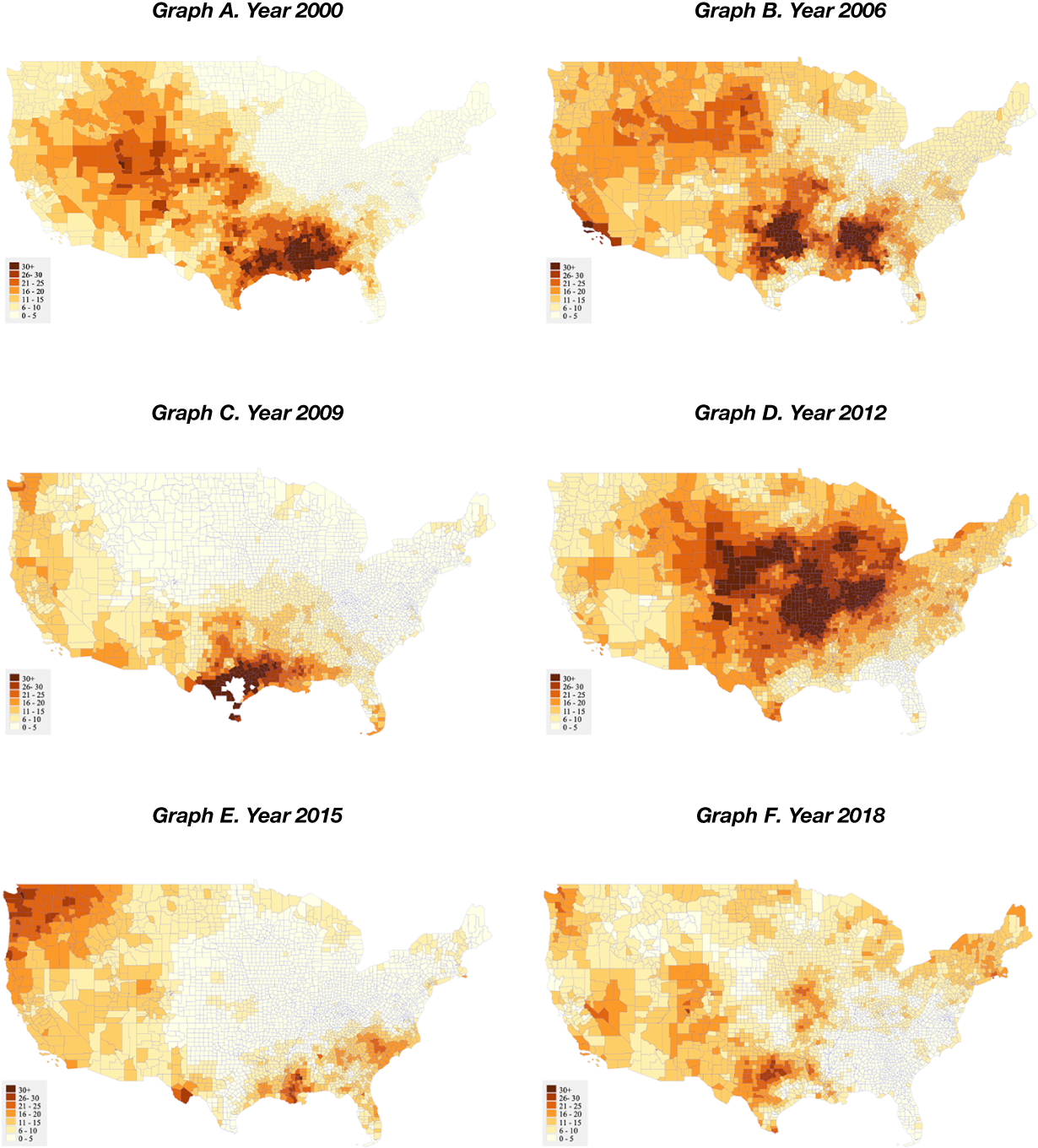
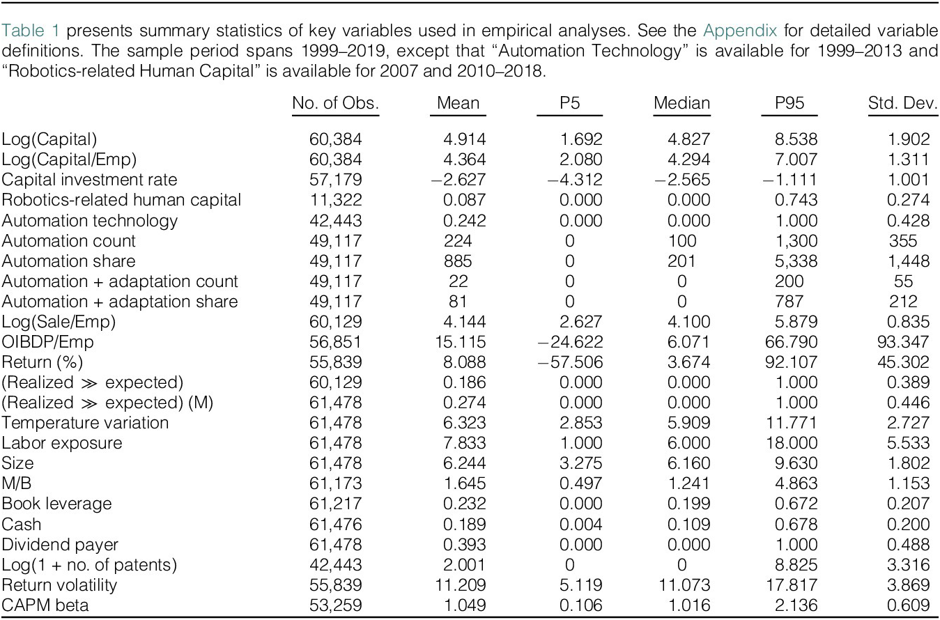
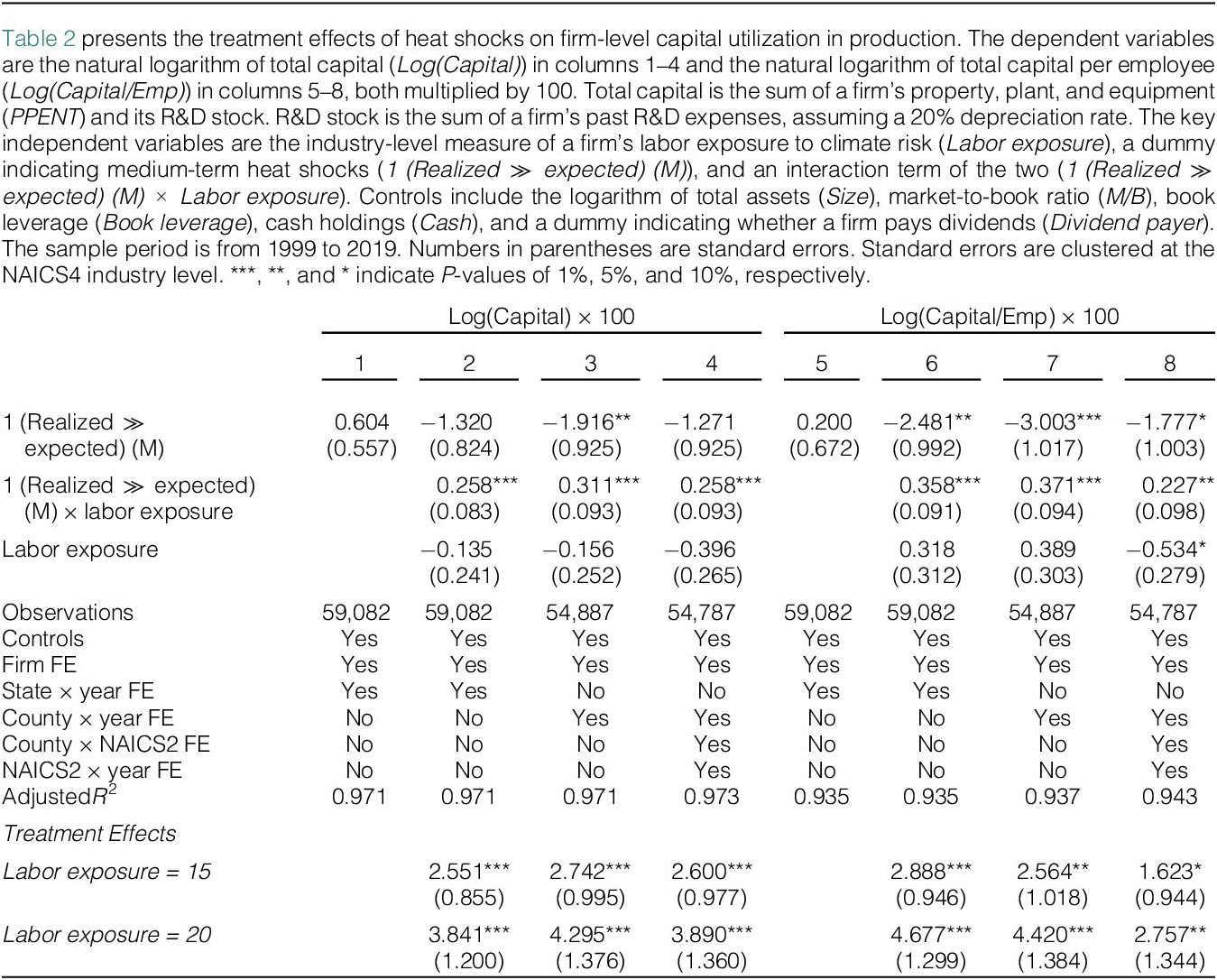
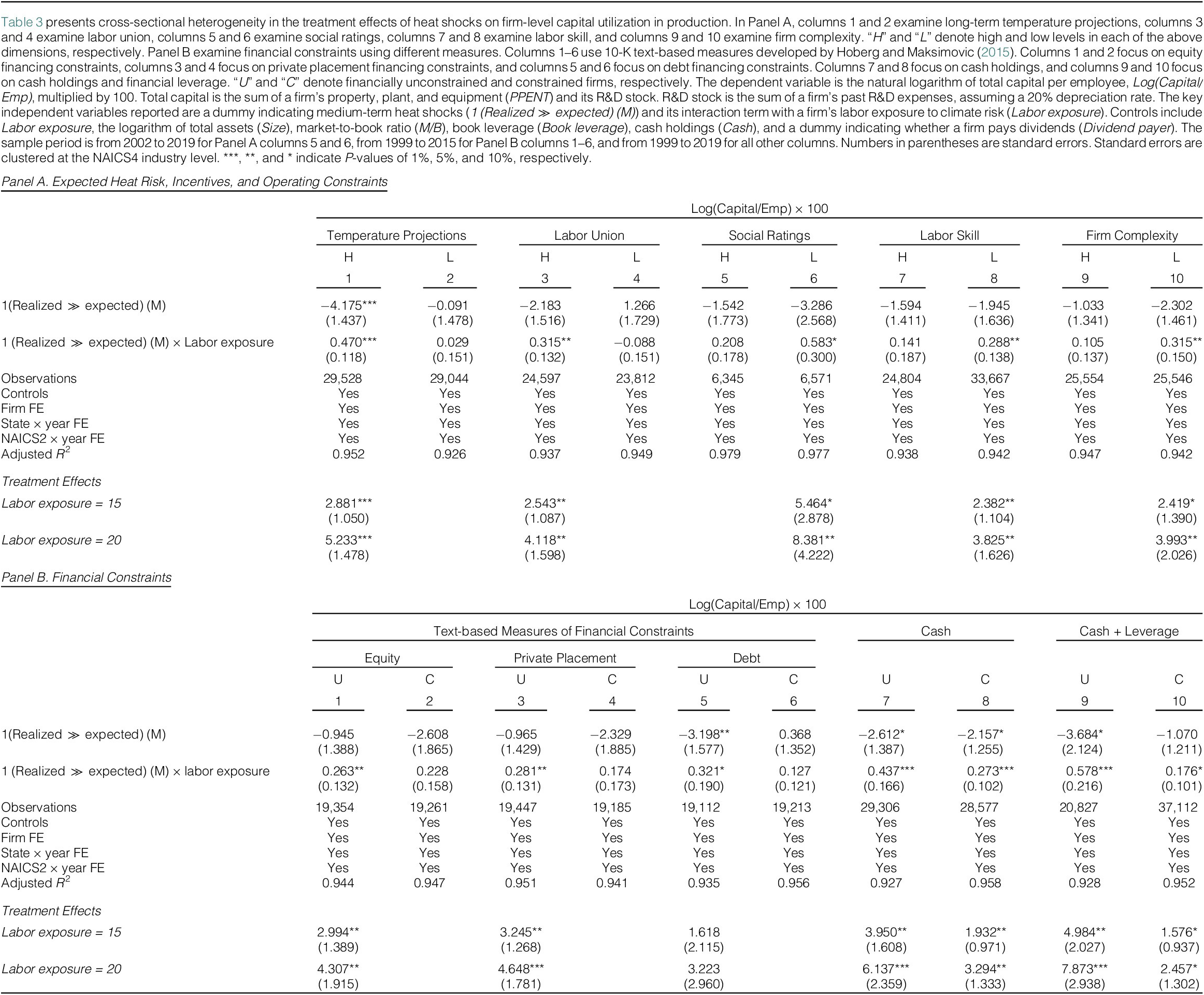
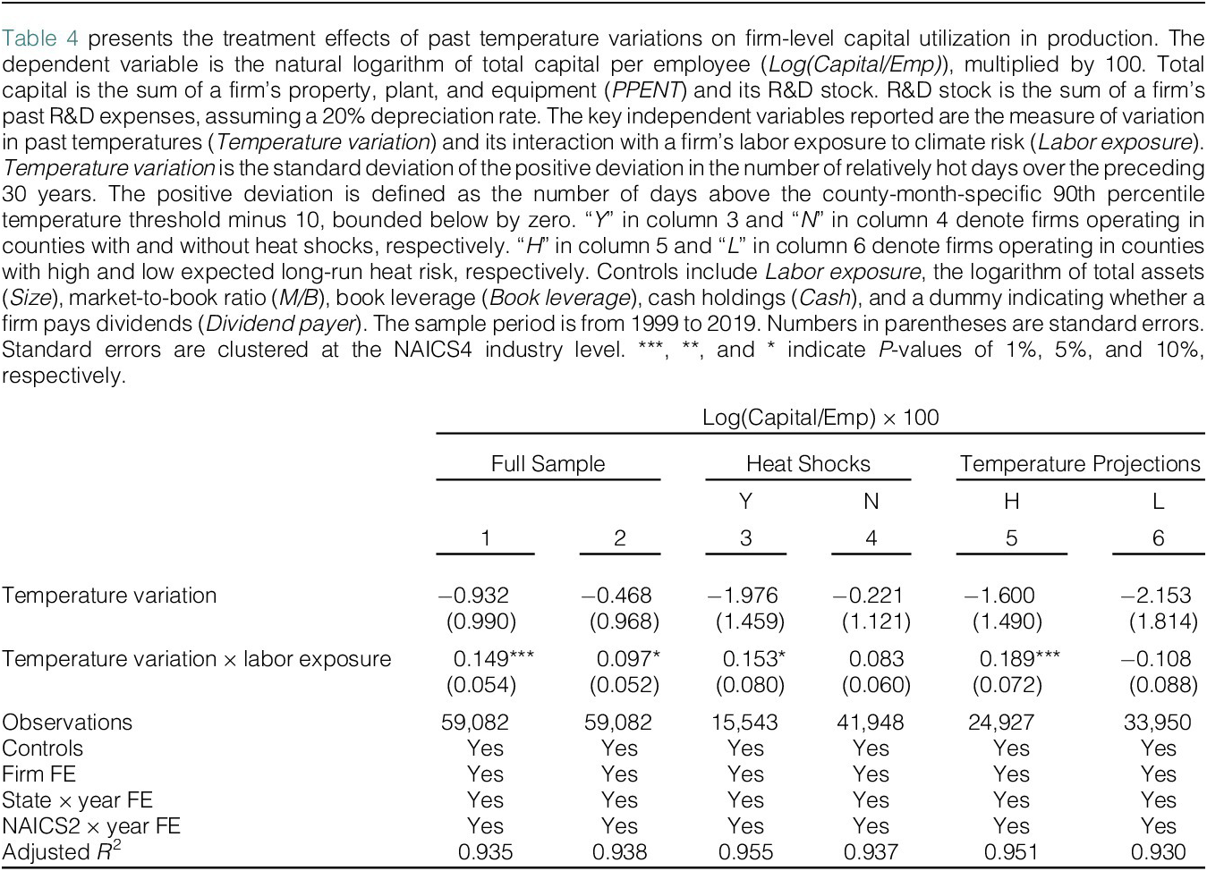
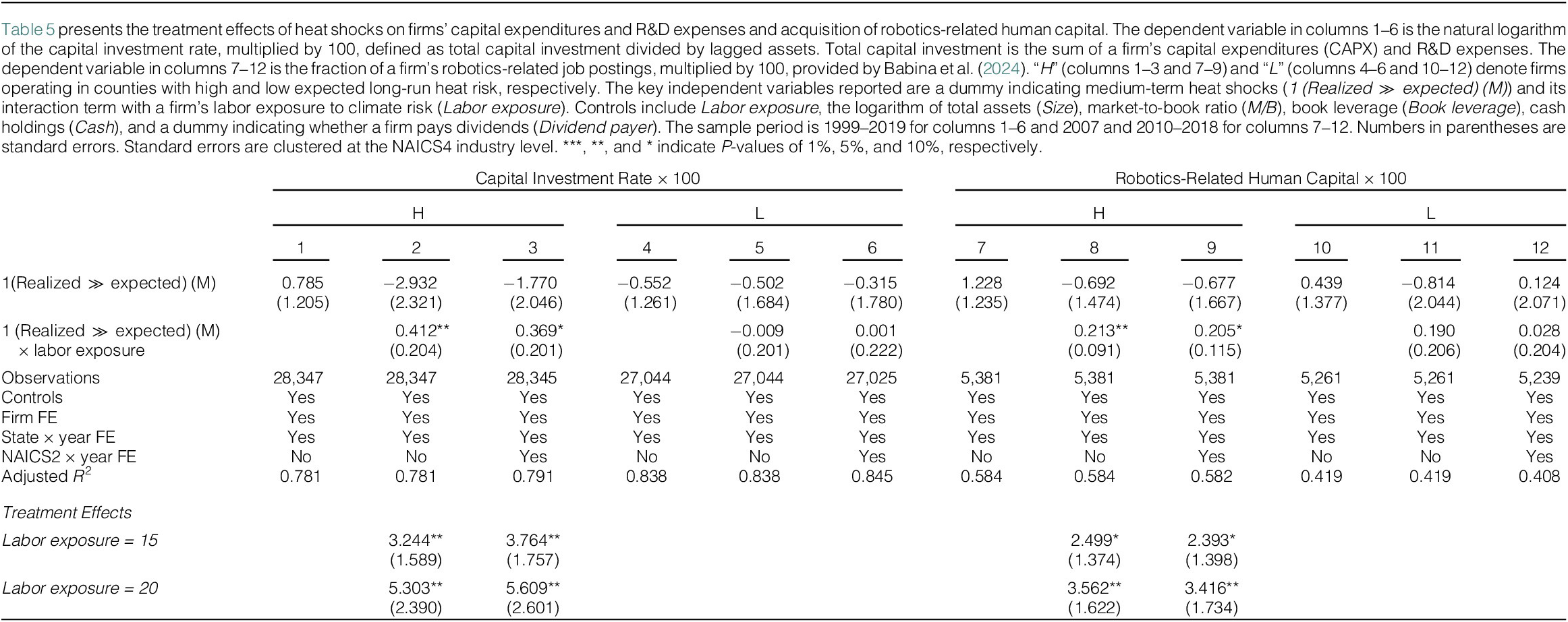
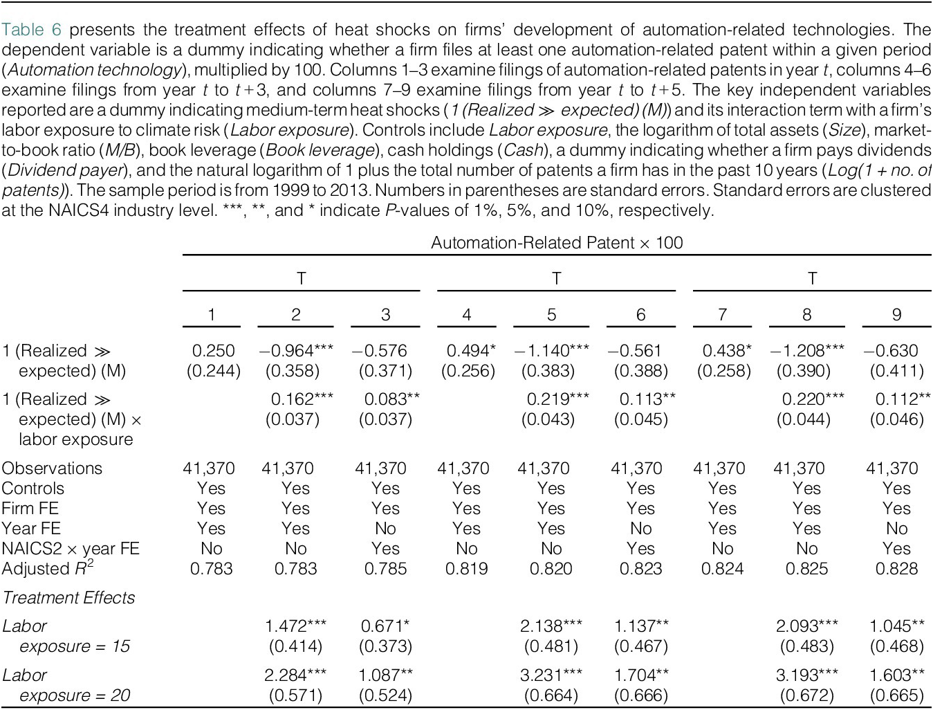
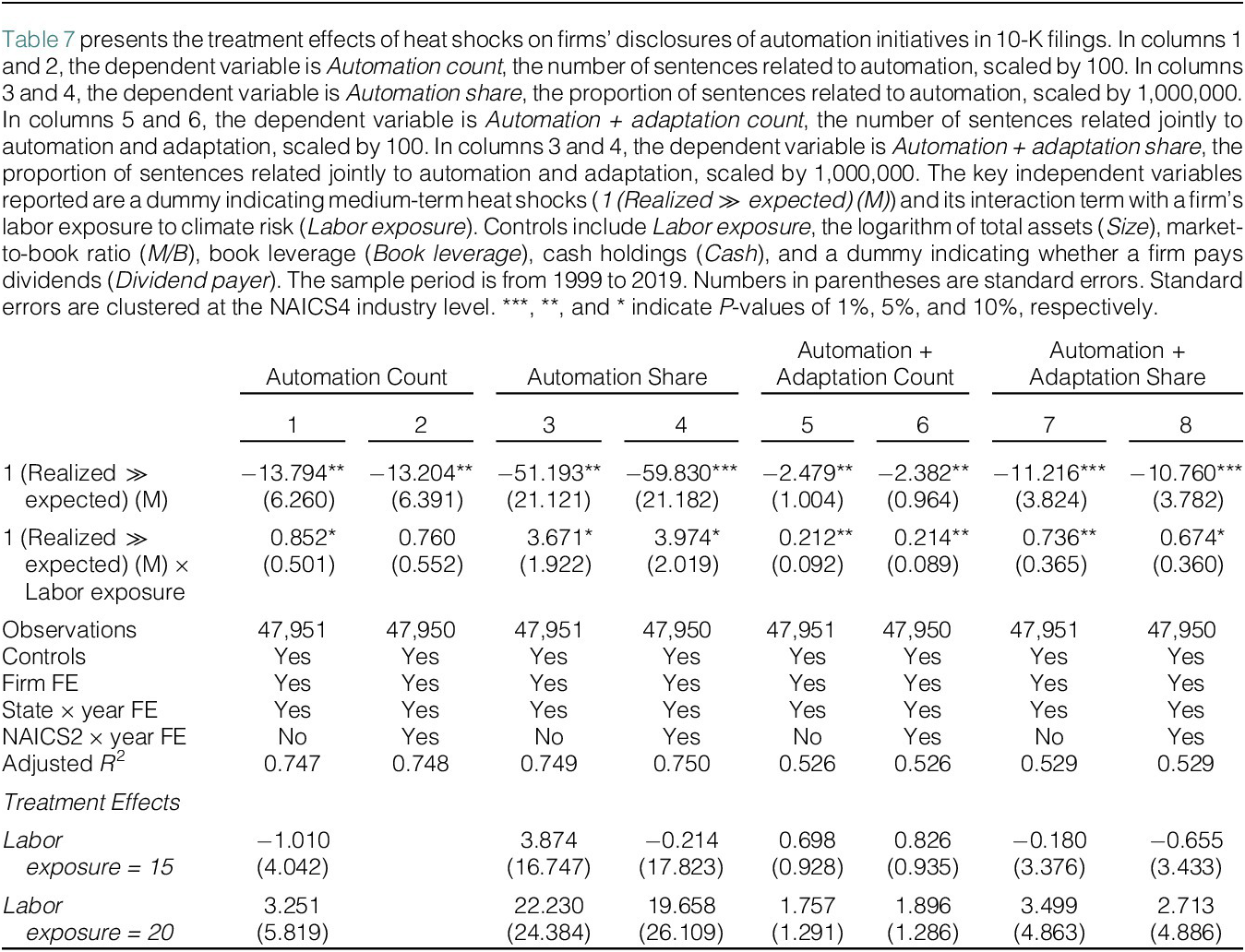
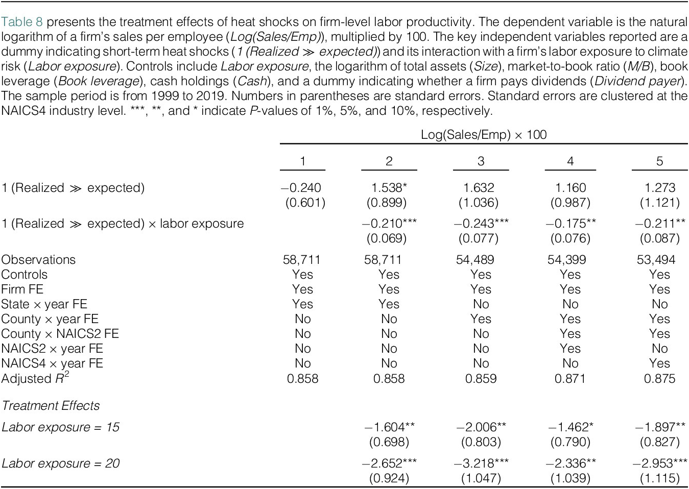
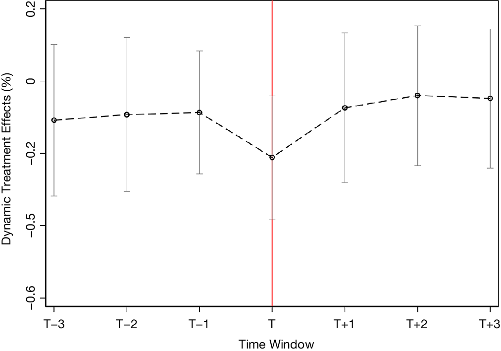
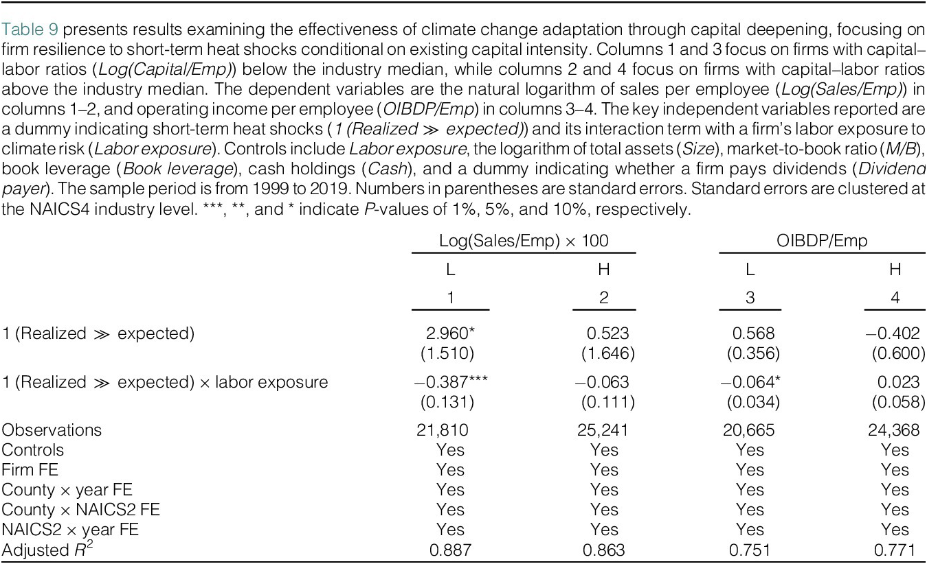
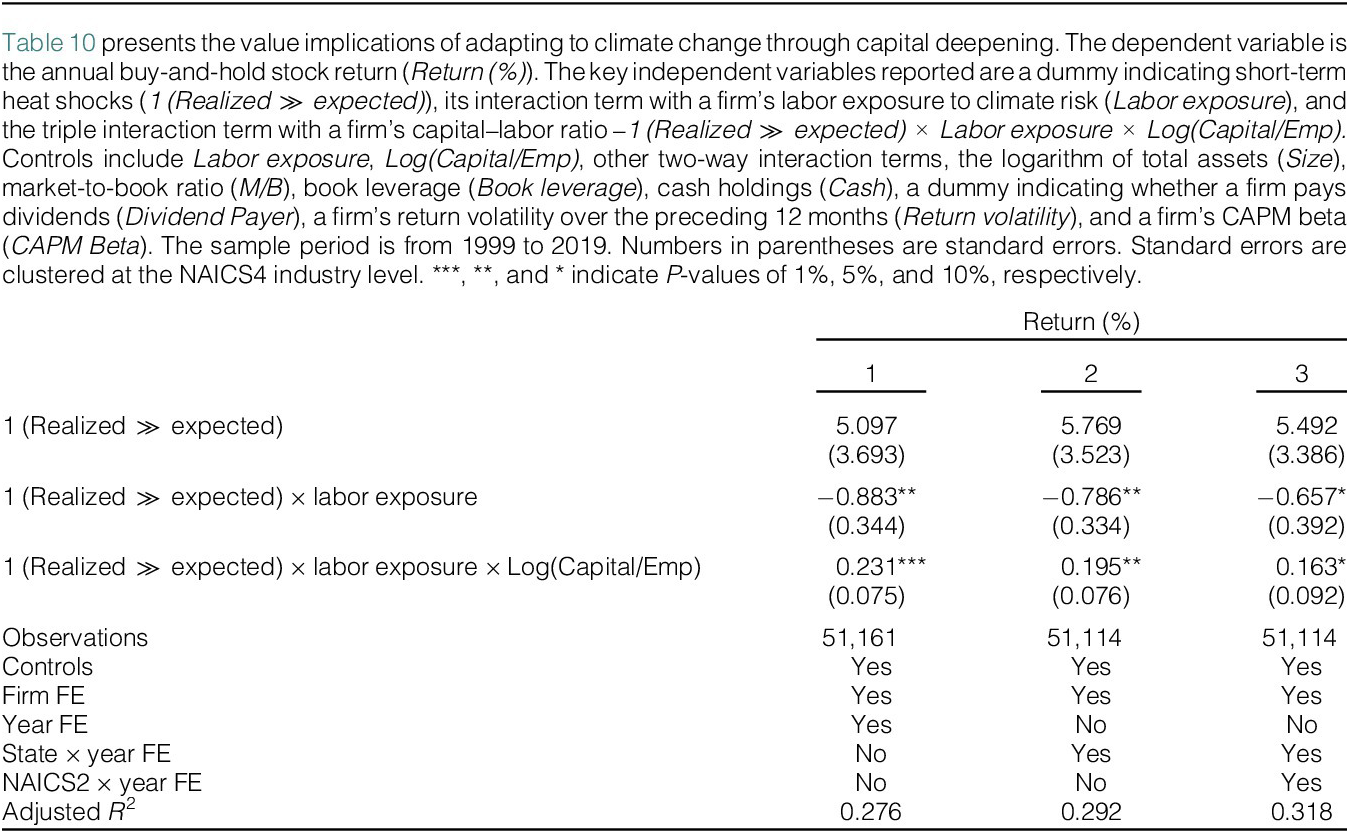


 Open access

