2.1. Flow simulation setting

Figure 1 shows the baseline computational model along with its key dimensions. A NACA0015 aerofoil is adopted as the wing section. The far-field boundary is positioned 30 $c$ from the wing, while a spanwise extent of 0.2 $c$ is sufficient to capture three-dimensional effects with minimal spanwise correlation (Deng, Jiang & Liu Reference Deng, Jiang and Liu2007; Jones, Sandberg & Sandham Reference Jones, Sandberg and Sandham2008; You & Moin Reference You and Moin2008; Gross & Fasel Reference Gross and Fasel2010). Owing to the early onset of flow separation near the leading edge at high angles of attack, the SJA is strategically positioned adjacent to the separation point to enhance flow control effectiveness (Amitay et al. Reference Amitay, Smith, Kibens, Parekh and Glezer2001; Yeh & Taira Reference Yeh and Taira2019; Wang, Li & Feng Reference Wang, Li and Feng2024). Accordingly, the jet orifice is located at the apex of the leading edge, with its spanwise position aligned with that of the wing. As the primary focus is on the external flow field, only the slot of the actuator is retained within the computational domain. In the present simulations, jet actuation is applied at the inner boundary – a modelling approach previously validated for its accuracy in reproducing the external flow characteristics of SJAs (Raju et al. Reference Raju, Aram, Mittal and Cattafesta2008; Ramos et al. Reference Ramos, Wolf, Yeh and Taira2019; Tousi et al. Reference Tousi, Coma, Bergadà, Pons-Prats, Mellibovsky and Bugeda2021). The exit width and length of the slot are both 0.008 $c$ . All simulations are conducted at a chord-based $ \textit{Re}$ of 2.1 $\times$ $10^5$ , with the wing set at an angle of attack $\alpha = 18^\circ$ .

Figure 1.

Schematic of the computational model and its geometrical dimensions.

Figure 2 shows the boundary condition set-up for the three-dimensional structured mesh. Periodic boundary conditions are applied at both spanwise ends to emulate an infinitely long wing. The far-field inflow is specified as a pressure far field, while all solid surfaces enforce a no-slip wall condition. The inner portion of the wall is represented by a velocity-inlet boundary, with the jet velocity prescribed as a sinusoidal function (Berk, Gomit & Ganapathisubramani Reference Berk, Gomit and Ganapathisubramani2016; Jankee & Ganapathisubramani Reference Jankee and Ganapathisubramani2021; Xu et al. Reference Xu, Long and Wang2023; Xu & Wang Reference Xu and Wang2024):

(2.1) \begin{align} u(t) = U_{\textit{max}} \sin (2\pi f t), \end{align}

where $U_{\textit{max}}$ is the peak jet velocity, $f$ is the excitation frequency and $t$ is the flow time. Additionally, the blowing ratio $C_B = U_{\textit{max}}/(\sqrt {2}U_\infty ) = 2.85$ . By setting this blowing ratio, the jet-induced vortex structures can be more clearly characterised. Moreover, under low-Reynolds-number aerofoil flow control conditions, this parameter exhibits good engineering feasibility.

The control frequency of the SJA is characterised by the following dimensionless parameter (Feero et al. Reference Feero, Lavoie and Sullivan2017; Itsariyapinyo & Sharma Reference Itsariyapinyo and Sharma2022; Kim et al. Reference Kim, Essel and Sullivan2022):

(2.2) \begin{align} F^+ = \frac {f c}{U_\infty }. \end{align}

To assess the impact of coherent vortical structures induced by the SJA on flow separation control, the excitation frequency is selected such that the non-dimensional frequency $F^+ = 1$ . This excitation generates dominant spanwise-coherent vortical structures within the flow field.

Figure 2.

Specification of the boundary conditions in the computational domain.

In this study, large-eddy simulations are employed to accurately capture the evolution of turbulent structures. The Semi-Implicit Method for Pressure-Linked Equations (SIMPLE) algorithm is adopted to ensure a robust coupling between the pressure and velocity fields. Under the adopted temporal discretisation, the SIMPLE algorithm provides stable and computationally efficient solutions for the unsteady simulations. Spatial discretisation of the gradient terms is performed using a least-squares cell-based scheme, while the momentum equations are discretised using a bounded central differencing approach to maintain high-order accuracy without introducing non-physical oscillations. Temporal discretisation is performed using a bounded second-order implicit scheme. Subgrid-scale turbulence is modelled using the kinetic-energy transport model proposed by Kim and Menon, wherein the subgrid-scale TKE is obtained by solving its transport equation (Kim & Menon Reference Kim and Menon1997):

(2.3) \begin{align} \rho \frac {\partial \widetilde {k}_{\textit{sgs}}}{\partial t} + \rho \frac {\partial \left(\widetilde {u}_{\kern-1pt j} \widetilde {k}_{\textit{sgs}}\right)}{\partial x_{\kern-1pt j}} = -\tau _{\textit{ij}} \frac {\partial \widetilde {u}_i}{\partial x_{\kern-1pt j}} - C_\epsilon \rho \frac {\widetilde {k}_{\textit{sgs}}^{3/2}}{\Delta _{\kern-1pt f}} + \frac {\partial }{\partial x_{\kern-1pt j}} \left ( \frac {\mu _t}{\sigma _k} \frac {\partial \widetilde {k}_{\textit{sgs}}}{\partial x_{\kern-1pt j}} \right ) \!, \end{align}

where $\rho$ denotes the fluid density, $\widetilde {k}_{\textit{sgs}}$ represents the subgrid-scale TKE and $\widetilde {u}$ are the filtered velocity components; $\tau _{\textit{ij}}$ is the subgrid-scale stress tensor; $C_\epsilon$ denotes a dimensionless model constant; $\Delta _{\kern-1pt f}$ is the filter width; $\mu _t$ is the turbulent viscosity; $\sigma _k$ denotes the turbulent Prandtl number for subgrid-scale kinetic energy; and $x_{\kern-1pt j}$ is the $j$ th spatial coordinate direction.

For the large-eddy simulations to be deemed reliable, the resolved TKE should exceed 80 % of the total TKE (Durbin Reference Durbin2001). Figure 3 shows the computed TKE distribution in the separated flow region on the leeward side of the aerofoil. The resolved TKE closely matches the total TKE in both magnitude and spatial distribution. Within the separation region, the resolved fraction exceeds 80 %, confirming that the chosen grid resolution satisfactorily meets the requirements for large-eddy simulations.

2.2. Verification and validation

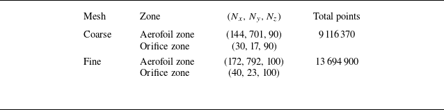
The grid sensitivity is verified using two grid configurations, as summarised in table 1. Both the aerofoil region and the actuator–cavity region are refined in the chordwise, spanwise and wall-normal directions. The coarse mesh comprises 9 116 370 grid points, whereas the fine mesh comprises 13 694 900 grid points. For both meshes, additional refinement is applied to the boundary-layer region and suction-side stall zone. The first-layer dimensionless grid height satisfies $\Delta y^+ = u_\tau \Delta y / \nu \lt 1$ (where $u_\tau$ is the local friction velocity, $\Delta y$ the normal distance from the first-layer node to the wall and $\nu$ the kinematic viscosity).

Table 1.

Summary of grids used in the numerical simulations.

Figure 3.

Validation of TKE statistics: (a) total TKE; (b) resolved TKE; (c) relative contribution.

Comparing the time histories of the aerodynamic loads before and after grid refinement shows that the time responses of the lift and drag coefficients on the coarse and fine meshes are in excellent agreement, as shown in figure 4. The amplitudes and temporal evolutions of the unsteady aerodynamic oscillations coincide closely.

Figure 4.

Grid-independence verification based on aerodynamic forces: (a) baseline; (b) controlled.

Figure 4. Long description

Two line graphs depict aerodynamic loads on an aerofoil in the stall regime, showing fluctuations due to characteristic frequencies in the flow field. Panel A: The line graph shows the baseline aerodynamic loads. The x-axis represents the dimensionless time U infinity t over c, and the y-axis on the left represents the lift coefficient C L, while the y-axis on the right represents the drag coefficient C D. The graph includes four data series: Fine-C L, Coarse-C L, Fine-C D, and Coarse-C D. The Fine-C L and Coarse-C L series show fluctuations in the lift coefficient, while the Fine-C D and Coarse-C D series show fluctuations in the drag coefficient. Panel B: The line graph shows the controlled aerodynamic loads. The x-axis represents the dimensionless time U infinity t over c, and the y-axis on the left represents the lift coefficient C L, while the y-axis on the right represents the drag coefficient C D. The graph includes four data series: Fine-C L, Coarse-C L, Fine-C D, and Coarse-C D. The Fine-C L and Coarse-C L series show fluctuations in the lift coefficient, while the Fine-C D and Coarse-C D series show fluctuations in the drag coefficient.

As shown in figure 5, a comparison between the two mesh configurations used to capture the time-averaged flow parameters reveals that the wall pressure coefficient and wall shear-stress distributions of the baseline flow are in near-perfect agreement, with the corresponding curves virtually overlapping. Consequently, the fine mesh is retained for all subsequent simulations to enable enhanced resolution of the vortical structures in the flow field.

Figure 5.

Time-averaged (a) wall pressure and (b) shear stress force grid-independence verification.

To further evaluate the accuracy of the present simulation in predicting the aerodynamic characteristics of aerofoils at low $ \textit{Re}$ , the numerical results are compared with experimental data obtained from the Walter H. Beech Memorial Wind Tunnel at Wichita State University, as reported by Sandia National Laboratories (Sheldahl & Klimas Reference Sheldahl and Klimas1981). The wind tunnel features a test section measuring 0.91 m in width and 2.13 m in height. Two representative flow conditions are considered for detailed comparison, corresponding to $ \textit{Re} = 1.6 \times 10^5$ and $ \textit{Re} = 3.6 \times 10^5$ . As shown in figure 6, the simulation demonstrates good agreement with experimental measurements in terms of predicting stall onset, capturing aerodynamic trends in the post-stall regime and reproducing overall aerodynamic force behaviour. These results confirm that the proposed method accurately captures the flow physics associated with symmetric aerofoils operating at low $ \textit{Re}$ .

Figure 6.

Case validation: (a) $ \textit{Re} = 1.6 \times 10^{5}$ ; (b) $ \textit{Re} = 3.6 \times 10^{5}$ .

Figure 6. Long description

Two line graphs compare experimental and simulated data for lift and drag coefficients at different angles of attack. Panel A: The graph shows data for a Reynolds number of 16w. The x-axis represents the angle of attack in degrees, ranging from -2 to 16 degrees. The left y-axis represents the lift coefficient (C_L), ranging from -0.3 to 0.9. The right y-axis represents the drag coefficient (C_D), ranging from 0 to 0.12. The black line with square markers represents the experimental lift coefficient (Exp - C_L - Re 16w), and the black line with circular markers represents the simulated lift coefficient (Sim - C_L - Re 16w). The red line with square markers represents the experimental drag coefficient (Exp - C_D - Re 16w), and the red line with circular markers represents the simulated drag coefficient (Sim - C_D - Re 16w). Panel B: The graph shows data for a Reynolds number of 36w. The x-axis represents the angle of attack in degrees, ranging from -2 to 18 degrees. The left y-axis represents the lift coefficient (C_L), ranging from -0.2 to 1.0. The right y-axis represents the drag coefficient (C_D), ranging from 0 to 0.15. The black line with square markers represents the experimental lift coefficient (Exp - C_L - Re 36w), and the black line with circular markers represents the simulated lift coefficient (Sim - C_L - Re 36w). The red line with square markers represents the experimental drag coefficient (Exp - C_D - Re 36w), and the red line with circular markers represents the simulated drag coefficient (Sim - C_D - Re 36w).

3.1. Coherent vortex structure generation

Figure 7 shows the instantaneous vortex structures before and after the application of control. In the baseline flow, a large separation region develops on the leeward side of the aerofoil, with the separation point located near the leading edge. Upon the introduction of jet control, the flow structure is substantially altered. Under periodic forcing, large-scale vortical structures with pronounced spanwise coherence emerge. Although the flow field exhibits characteristic multi-scale vortical structures, the coherent spanwise vortices account for a larger share of the kinetic energy and play a dominant role in the reorganisation of the separated region. Accordingly, the following analysis focuses on quantifying their contribution to flow control effectiveness and elucidating the associated physical mechanisms.

The characteristic alternating blowing–suction mechanism of the SJA induces the formation of two distinct sets of spanwise-oriented vortices. Vortices generated during the blowing phase predominantly occupy the outer region of the flow and are referred to as BIVs, whereas those generated during the suction phase form closer to the wall and are termed SIVs. This alternating actuation results in the periodic appearance of BIVs and SIVs throughout the cycle. Additionally, an analysis of the velocity field indicates that the energy associated with BIVs remains approximately constant during downstream development, whereas the energy of SIVs decays more rapidly.

Figure 7.

Instantaneous vortex structures contoured by velocity using $Q^* = Q c^2 / U_\infty = 200$ : (a) baseline; (b) $1/4T$ ; (c) $2/4T$ ; (d) $3/4T$ ; (e) $4/4T$ .

Figure 8 shows the formation processes of distinct vortex structures during the blowing and suction phases. During the blowing phase, the backward-directed jet impinges on the incoming free stream, actively inducing the formation of separation vortices (BIVs). By contrast, during the suction phase, the suction flow inhibits the development of the free stream near the leading edge of the aerofoil, resulting in the formation of a small-scale localised separation region within which SIVs are generated. A comparative analysis indicates significant differences in the formation mechanisms of BIVs and SIVs. The BIVs are primarily generated from the direct impingement of the jet on the free stream, leading to strong energy injection and a relatively high overall energy level. By contrast, the formation of SIVs is attributed to the blockage effect exerted by the suction flow on the incoming stream. Consequently, SIVs exhibit smaller scales and lower energy levels than BIVs.

Figure 8.

Mechanism of coherent vortex formation: (a) BIVs; (b) SIVs.

3.2. Vortex trajectories and characteristics

Figure 9 shows vorticity contours depicting the evolution of vortical structures over a complete SJA cycle. The results demonstrate the alternating emergence of large-scale BIVs and SIVs on the leeward side, with the flow field exhibiting pronounced spanwise coherence. These coherent vortices are associated with regions of elevated vorticity. Notably, the SIVs experience a rapid decay in vorticity strength as they convect downstream. Conversely, the BIVs maintain a higher vorticity intensity and can sustain energy more effectively throughout their downstream evolution.

Figure 9.

Evolution of spanwise-averaged vorticity field within the control cycle. The orange line represents $Q^*=200$ : (a) $1/4T$ ; (b) $2/4T$ ; (c) $3/4T$ ; (d) $4/4T$ .

Figure 10.

Vortex structures identified using the $Q_s$ criterion, where the black lines represent the boundaries of the vortices.

To further quantify the trajectories and overall strengths of the coherent vortices, circulation is employed as a measure of their energy levels. However, with regard to the identification of vortex boundaries, the $Q$ criterion remains one of the most widely adopted methods. Despite its popularity, the extracted vortex boundaries are highly sensitive to the choice of threshold, which may introduce uncertainty in quantitative analyses.

To address this limitation, the $Q_s$ method is introduced (Kovács & Kristóf Reference Kovács and Kristóf2025). Compared with the classical $Q$ criterion, the $Q_s$ approach incorporates vorticity-based coherence weighting and statistical thresholding via a Gaussian mixture model. This framework enables an adaptive, data-driven identification process that does not rely on empirically prescribed thresholds, thereby providing a more robust and physically consistent delineation of vortex boundaries. Figure 10 presents the results of vortex identification based on the $Q_s$ method.

Based on the extracted effective vortex boundaries, the circulation and trajectories of the vortices are further evaluated, and the corresponding formulation is given as follows:

(3.1) \begin{align} \varGamma = \iint \limits _D \omega \, {\rm d}S, \\[-28pt] \nonumber \end{align}

(3.2) \begin{align} x_c = \frac {1}{\varGamma } \iint \limits _D \omega x \, {\rm d}S , \\[-28pt] \nonumber\end{align}

(3.3) \begin{align} y_c = \frac {1}{\varGamma } \iint \limits _D \omega y \, {\rm d}S, \\[0pt] \nonumber \end{align}

where $D$ denotes the integration domain enclosed by the vortex boundary and $(x_c, y_c)$ represents the location of the vortex centre.

Compared with the SIVs, the BIVs are located farther from the wall and exhibit a higher overall vorticity strength (figure 11). This trend is primarily attributed to the more effective energy injection associated with the blowing phase of the SJA, whereas the SIVs formed through the blockage effect of the jet have relatively weaker strength. As the flow develops downstream, the circulation strengths of both BIVs and SIVs gradually decrease. Near the trailing edge of the aerofoil, the overall energy of the SIVs is substantially reduced, whereas the BIVs can sustain relatively high energy levels. Furthermore, the increase in the wall-normal displacement and overall weakening of the vortex strength lead to a diminished influence of both vortex types on the wall in the mid-to-aft region of the aerofoil.

Figure 11.

Trajectory of coherent vortex and evolution of circulation.

Figure 12.

(a,b) Frequency–space and (c,d) wavenumber–frequency spectra of normal velocity fluctuations $v'$ along the vortex trajectory. Dashed white line is the convective ridge: (a,c) BIVs; (b,d) SIVs.

To further quantify the spectral characteristics and streamwise development of the BIVs, 200 measurement points are evenly distributed along the trajectories of the coherent vortices. The normal velocity fluctuations at these points are recorded for spectral analysis. Figure 12 presents both the frequency-domain spectra at various streamwise positions and the corresponding wavenumber–frequency spectra. The frequency spectra are computed using the Welch method. This approach is adopted to obtain a statistically stable estimate of the power spectral density by reducing the variance of the periodogram through segment averaging. The segment length is set to Nperseg = 512, which provides a balanced compromise between frequency resolution and the number of segments available for ensemble averaging. A 75 % overlap is applied to further improve the robustness and smoothness of the spectral estimates. The resulting non-dimensional time–frequency resolution is 0.2. The wavenumber–frequency spectra are obtained by applying a two-dimensional fast Fourier transform to the space–time matrix, with a non-dimensional wavenumber resolution of 5.3 and a time–frequency resolution of 0.005. The results indicate that, across all streamwise locations, the energy is concentrated around the actuation frequency and its harmonics, demonstrating a frequency lock-in behaviour for both BIVs and SIVs. Additionally, along the SIV trajectory, the harmonic energy weakens as the vortices convect towards the trailing edge, whereas the BIVs maintain higher energy levels throughout their evolution. These findings are consistent with the circulation strength analysis presented earlier. Furthermore, the wavenumber–frequency spectra reveal that the dominant energy is aligned along a line of fixed slope, commonly referred to as the convective ridge (Kurelek, Yarusevych & Kotsonis Reference Kurelek, Yarusevych and Kotsonis2019), corresponding to a constant convection velocity that satisfies

(3.4) \begin{align} U_{\textit{con}} = 2\pi f / k. \end{align}

The convection velocity of the coherent vortices is approximately $U_{\textit{con}} \approx U_\infty$ , demonstrating that the BIVs and SIVs convect downstream at a speed close to the free-stream velocity. This finding suggests that the motion of the coherent structures is primarily governed by the free-stream flow and co-evolves with the mainstream.

To further compare the mean vorticity distributions before and after control, figure 13 shows the comparative results. In the baseline flow, the presence of a large-scale separation region induces a pronounced wall-normal lift-off of the high-vorticity layer, beginning near the leading edge. Simultaneously, the low-energy fluid motion within the separation zone results in relatively low vorticity levels near the wall. In the controlled flow field, the structure is significantly modified. Notably, the wall-normal displacement of the high-vorticity region is substantially reduced, indicating that the control strategy effectively suppresses boundary-layer separation and promotes the maintenance of elevated near-wall vorticity levels.

Figure 13.

Spanwise-averaged mean vorticity analysis before and after control: (a) baseline; (b) controlled. The dotted lines represent the trajectory of the vortices.

Figure 14.

Contours of the mean vorticity distribution: (a) $ \textit{MSR}$ ; (b) $\textit{VD}$ ; (c) $ \textit{TT}$ ; (d) $ \textit{FSS}$ . The dotted lines represent the trajectory of the vortices.

To further investigate the generation mechanisms of mean vorticity in the controlled flow field, an analysis based on the mean vorticity equation is conducted. The equation is given as follows:

(3.5) \begin{align} \frac {\partial \overline {\omega }_i}{\partial t} + \overline {u}_{\kern-1pt j} \frac {\partial \overline {\omega }_i}{\partial x_{\kern-1pt j}} = \underbrace {\overline {\omega }_j \overline {s}_{\textit{ij}}}_{\textit{MSR}} + \underbrace {\nu \frac {\partial ^2 \overline {\omega }_i}{\partial x_{\kern-1pt j} \partial x_{\kern-1pt j}}}_{\textit{VD}} - \underbrace {\frac {\partial \overline {u_j'\omega _i'}}{\partial x_{\kern-1pt j}}}_\textit{{TT}} + \underbrace {\overline {\omega _j' s_{\textit{ij}}'}}_{\textit{FSS}}, \end{align}

where $s$ is the strain-rate tensor and $\textit{ij}$ represents the different directions.

In this equation, each term represents the influence of different physical mechanisms on the evolution of the mean vorticity (Wang et al. Reference Wang, Qu, Sun and Bai2023; Tang et al. Reference Tang, Sun, Yan, Wang, Yu, Huang, Wang and Zhu2024). The first term $ \textit{MSR}$ describes the rate of the mean vorticity generation owing to the mean strain rate. The second term $\textit{VD}$ represents the viscous diffusion of the mean vorticity resulting from the fluid motion. The third term $ \textit{TT}$ reflects the transport of mean vorticity by turbulent velocity fluctuations, whereas the fourth term $ \textit{FSS}$ characterises the stretching of vortex tubes induced by fluctuating strain rates, thereby generating mean vorticity.

Based on the contour distribution analysis shown in figure 14, the vorticity generation rate associated with the $ \textit{MSR}$ is relatively high at both the leading and trailing edges on the leeward side. At the leading edge, the persistent jet leads to significant gradients in the flow field, whereas the trailing edge is influenced by vortex-shedding phenomena, resulting in enhanced vorticity production. Regarding the $\textit{VD}$ , its intensity is mainly concentrated near the wall regions. Although viscous diffusion is prominent in the near-wall area, its overall contribution to the mean vorticity remains relatively minor.

The $ \textit{TT}$ and $ \textit{FSS}$ exhibit stronger magnitudes at the leading edge, with overall amplitudes greater than those of the first two terms. This indicates that turbulent velocity fluctuations and fluctuating strain rates have a significant impact on the transport and generation of spanwise mean vorticity. Notably, the third term shows strong distribution characteristics at the leading edge and exhibits elongated, strip-like structures along the trajectories of the BIVs and SIVs across the leeward surface. By contrast, the structures near the trailing edge are relatively fragmented, which is closely related to the traces left by the motion of the coherent vortices over the leeward side.

4.1. Instantaneous aerodynamic load modulation

Figure 15 shows the time–frequency evolution characteristics of the lift coefficient before and after the control. In the baseline flow, owing to the influence of wake instabilities, the lift fluctuation frequency is primarily governed by the vortex-shedding frequency, which corresponded to a dimensionless frequency of $ \textit{St} \approx 0.6$ . After the control is applied, the lift fluctuation frequency underwent a significant shift, aligning with the excitation frequency and exhibiting a distinct lock-in behaviour. Furthermore, as observed from the time histories of the lift load presented previously, the fluctuation characteristics become more orderly, demonstrating pronounced coherence.

Figure 15.

Time–frequency evolution of the lift coefficient $C_L$ before and after control: (a) baseline; (b) controlled.

Figure 16 shows the evolution of the pressure contours during the excitation control process. Owing to their relatively high energy, BIVs generate a pronounced negative pressure effect during downstream evolution. However, as BIVs convect downstream, their structures gradually move away from the wall surface, resulting in a diminishing influence on the wall pressure over the aft portion of the aerofoil chord. By contrast, SIVs that remain closer to the wall possess a lower overall energy. Consequently, the associated low-pressure regions are smaller in both area and intensity. Moreover, the pressure deficit induced by the SIVs decays rapidly along the streamwise direction and becomes negligible near the trailing edge, implying a limited contribution to surface suction enhancement.

Figure 16.

Evolution of the spanwise-averaged pressure coefficient field within the control cycle. The black line represents $Q^*=200$ and the dotted lines represent the trajectory of the vortices: (a) $1/4T$ ; (b) $2/4T$ ; (c) $3/4T$ ; (d) $4/4T$ .

Figure 17 shows the spatiotemporal evolution of the surface pressure over the upper side of the aerofoil. Owing to the sustained excitation by the leading-edge jet, a persistent low-pressure region is maintained from the leading-edge apex to approximately $x/c = 0.2$ , resulting in a marked increase in suction near the leading edge. This observation is consistent with a previous analysis of the time-averaged pressure envelope. Additionally, both BIVs and SIVs are accompanied by the formation of low-pressure ridges along their motion trajectories. The BIVs, which are characterised by higher energy, exert a pronounced influence on the leading-edge region. However, as their trajectories gradually diverge from the wall surface, their impact on the pressure field weakens significantly beyond $x/c = 0.4$ . By contrast, SIVs with a lower overall energy decay rapidly in the downstream direction. Their contribution to the pressure reduction is weaker than that of the BIVs, and by $x/c = 0.4$ , their influence on the upper surface pressure becomes limited.

Figure 17.

Spatiotemporal evolution of the pressure coefficient on the upper surface.

4.2. Mean aerodynamic load modulation

A further comparison of the time-averaged pressure distributions before and after flow control is presented in figure 18. In the baseline flow, the large-scale flow separation results in a significantly reduced pressure gradient over the upper surface of the aerofoil, yielding a nearly uniform pressure distribution and the formation of a characteristic pressure plateau. Upon the application of flow control, the flow-field structure is effectively improved, leading to a substantial enhancement in the mean suction peak from the leading-edge apex to $x/c = 0.2$ . Although the suction is slightly reduced near the trailing edge owing to the confinement of the separated vortices, the increase in pressure difference at the leading edge contributes more significantly to the lift enhancement. As shown in figure 4, the implementation of the control increases the average lift coefficient from 0.763 to 1.069, while reducing the average drag coefficient from 0.331 to 0.163, thereby substantially enhancing the aerodynamic performance.

Figure 18.

Comparison of the spanwise-averaged mean pressure field before and after control: (a) distribution of the surface pressure coefficient; (b) pressure coefficient contour in the baseline field; (c) pressure coefficient contour in the controlled field.

Regarding the fluctuations in aerodynamic loads, the SJA control leads to a slight increase in lift-load oscillations, with root-mean-square (RMS) $C_L$ rising from 0.118 to 0.136, while the drag-load fluctuations are reduced, as indicated by the decrease in RMS $C_D$ from 0.037 to 0.017. Figure 19 further shows the distribution of the RMS values of the pressure fluctuations before and after control. The range of strong pressure fluctuations differs significantly. In the baseline flow, wake instabilities dominate the pressure fluctuation distribution, resulting in pronounced fluctuations near the trailing edge. In the controlled flow field, the separated flow region is effectively suppressed, leading to a significant reduction in pressure fluctuations at the trailing edge. The regions of strong pressure fluctuations shift towards the leading edge and along the trajectories of the BIVs. This observation further indicates that the BIVs decay more slowly during their downstream evolution, whereas the SIVs can maintain relatively high energy levels only near the leading edge. As the BIVs convect downstream and lift away from the wall, their influence on surface pressure fluctuations gradually weakens.

This phenomenon demonstrates that the SJA, acting as a periodic input, can effectively generate high-energy coherent structures to enhance surface suction. However, this process may also induce localised amplification of pressure fluctuations. Future studies will further adjust the jet energy and optimise BIV trajectories to achieve the desired control effects, which mitigate aerodynamic force oscillations while minimising the extent of additional pressure fluctuation regions.

Figure 19.

Comparison of the RMS pressure field before and after control: (a) baseline; (b) controlled. The dotted lines represent the trajectory of the vortices.

5.1. Three-dimensional decomposition

In the conventional turbulence decomposition, the flow variables are separated into a time-averaged (mean) component $\bar {f}$ and a fluctuating component $f^\prime$ . In this study, the SJA induces large-scale coherent structures. Triple decomposition is applied to further investigate the coherence in the flow field. The fluctuating component is further divided into coherent $\widetilde {f}$ and turbulent $f^{\prime \prime }$ components (Hussain & Reynolds Reference Hussain and Reynolds1970; Sato et al. Reference Sato, Nonomura, Okada, Asada, Aono, Yakeno, Abe and Fujii2015; Yang, Ekmekci & Sullivan Reference Yang, Ekmekci and Sullivan2022), expressed as follows:

(5.1) \begin{align} f(x,t) = \underbrace {\bar {f}(x)}_{\text{mean}} + \underbrace {f'(x,t)}_{\text{fluctuation}} = \underbrace {\bar {f}(x)}_{\text{mean}} + \underbrace {\widetilde {f}(x,t)}_{\text{coherent}} + \underbrace {f''(x,t)}_{\text{turbulent}}. \end{align}

Notably, the time-averaged component $\bar {f}$ is obtained through

(5.2) \begin{align} \bar {f}(x) = \lim _{T \rightarrow \infty } \frac {1}{T} \int \limits _0^T f(x,t) \, \mathrm{d}t, \end{align}

where the averaging period satisfies $U_\infty T/c = 20$ to approximately ensure statistical convergence of the mean flow characteristics.

Equation (5.3) presents the principle for obtaining the phase-averaged flow field. For transient flows with quasi-periodic characteristics, multiple sets of instantaneous flow-field data are acquired at fixed time intervals $\tau$ corresponding to a specific phase $\phi$ . The turbulent fluctuation components are filtered using an ensemble average. Owing to the pronounced periodicity observed under the SJA, the time interval $\tau$ is selected to match the actuation period in subsequent analysis.

(5.3) \begin{align} \langle f(x,t) \rangle _\phi = \lim _{N \rightarrow \infty } \frac {1}{N} \sum _{n=0}^{N} f(\phi + n\tau ). \end{align}

By subtracting the time-averaged flow field from the phase-averaged flow field, the coherent component can be extracted as

(5.4) \begin{align} \widetilde {f}(x,t) = \langle f(x,t) \rangle _{\phi } - \bar {f}(x). \end{align}

5.2. Direct momentum addition

Regarding energy transfer, the jet introduces a high-momentum fluid into the separated recirculation region, significantly improving the adverse pressure gradient distribution near the separation point of the boundary layer, thereby suppressing flow separation. Figure 20 shows the contours of the normal coherent and turbulent velocity fluctuations over one control cycle. The results show that along the evolutionary path of the BIVs, the intensity of the coherent normal velocity fluctuations remains pronounced, and their energy is largely conserved along the streamwise direction. By contrast, the SIVs exhibit weaker overall fluctuation energy, which decays rapidly downstream and becomes negligible near the trailing edge. Moreover, the magnitude of the turbulent velocity component is generally lower throughout the cycle. This further indicates that coherent fluctuations dominate the downstream development of coherent structures and play a direct role in the energy transport towards the separation region.

Figure 20.

Evolution of the coherent and turbulent velocity fields within the control cycle. The black line represents $Q^*=200$ and the dotted lines represent the trajectory of the vortices. (a–d) Coherent velocity $1/4T$ to $4/4T$ ; (e–h) turbulent velocity $1/4T$ to $4/4T$ .

To further analyse the TKE characteristics of the controlled flow field, the TKE is decomposed into coherent and turbulent components using $({1}/{2}) \overline {u_i' u_i'} = ({1}/{2}) \overline {\tilde {u}_i \tilde {u}_i} + ({1}/{2}) \overline {\hat {u}_i \hat {u}_i}$ (Feng & Wang Reference Feng and Wang2012; Xu & Wang Reference Xu and Wang2024). The results indicate that, under the influence of an SJA, the TKE is primarily concentrated in the leading-edge region of the aerofoil, where direct jet impingement leads to significant velocity fluctuations (figure 21). This distribution is consistent with the RMS contours of the pressure. Upon decomposition, it is evident that the proportion of the coherent TKE is substantially higher than that of the turbulent component, indicating that coherent structures predominantly govern fluctuations in the flow field.

Figure 21.

Decomposition of TKE in the controlled flow.

5.3. Free-stream momentum entrainment

Owing to its distinctive periodic perturbation characteristics, the SJA exhibits a more pronounced entrainment effect on flow control. The unsteady vortex structures induced by the jets effectively drive the momentum exchange between the outer and inner regions of the boundary layer, thereby enhancing fluid mixing. The Reynolds shear stress is a fundamental concept in fluid dynamics for characterising the influence of turbulence on momentum transport. In this study, the entrainment effect of the coherent structures induced by the control is examined by analysing the Reynolds shear stress. Figure 22 shows that in the baseline flow field, the separated region spans the entire upper wing surface, causing airflow to lift at the leading edge. Consequently, a distinct Reynolds shear-stress component is observed along the separation boundary line near the leading edge. Additionally, vortex shedding near the trailing edge contributes to the strong Reynolds stress magnitudes in this region. After the control is applied, the Reynolds stress distribution changes significantly, the stress streaks in the leading-edge separation region shift downward and strong shear-stress components appear along the trajectory of the BIVs, with the lengths of these streaks spanning nearly the entire chord. By contrast, SIVs play a minor role in the flow mixing near the mid- to trailing edges of the aerofoil. Overall, the BIVs induced by the SJA significantly enhance the momentum exchange between the fluid inside and outside the separated flow region on the suction side, which is consistent with the previously discussed results.

Figure 22.

Comparison of Reynolds stress distributions before and after control: (a) baseline; (b) controlled. The dotted lines represent the trajectory of the vortices.

Further triple decomposition analysis is conducted to examine the Reynolds shear-stress dynamics in a controlled flow field (Hussain & Reynolds Reference Hussain and Reynolds1970; Sato et al. Reference Sato, Nonomura, Okada, Asada, Aono, Yakeno, Abe and Fujii2015). Figure 23 shows that the coherent Reynolds shear-stress component is more prominent, with its overall distribution closely matching that of the total Reynolds shear stress. This finding indicates that the coherent component plays a dominant role in flow mixing and has a more pronounced influence on momentum transfer.

Figure 23.

Decomposition of the Reynolds shear stress in the controlled flow.

To further investigate the entrainment mechanism of the coherent component associated with BIVs, a quadrant analysis of the Reynolds stress is conducted by statistically classifying the instantaneous states of the streamwise and wall-normal coherent velocity fluctuations. This approach quantifies the contributions of different turbulent events to momentum transport (Wallace Reference Wallace2016). Here Q1 ( $u' \gt 0$ , $v' \gt 0$ ) corresponds to outwards interaction, Q2 ( $u' \lt 0$ , $v' \gt 0$ ) to ejection, Q3 ( $u' \lt 0$ , $v' \lt 0$ ) to inward interaction and Q4 ( $u' \gt 0$ , $v' \lt 0$ ) to sweep. The positions of the measurement points (A and B) are shown in figure 23. The quadrant analysis at the measurement point, as shown in figure 24, reveals a clear bias towards Q2 and Q4. Furthermore, the covariance integrand indicates that the Q2 component is dominant, suggesting that the entrainment behaviour of BIVs is primarily governed by ejection events. The key characteristic of this process is the outward entrainment and transport of the low-energy fluid from the near-wall region to the outer stream, which significantly reduces the extent of the separated recirculation zone. Given that the coherent vortex resides in a local low-pressure region, its induced flow can be likened to a ‘suction pump’, exhibiting a strong capacity to attract and capture low-momentum fluid packets.

Figure 24.

Quadrant analysis of Reynolds stress associated with coherent velocity components: (a) joint probability distribution of point A; (b) joint probability distribution of point B; (c) covariance integrand distribution of point A; (d) covariance integrand distribution of point B.

Figure 25 shows that throughout the control cycle, the coherent vortices exhibit a pronounced coherent shear-stress intensity, forming a characteristic quadrupolar rotational pattern. This phenomenon is particularly evident in quasi-two-dimensional flow fields. The coherent-stress component is more prominent than the turbulent-shear-stress component. As BIVs evolve downstream, the spatial extent and overall intensity of the coherent Reynolds shear stress remain consistently high. However, the stress induced by SIVs is only significant in the fore- to mid-chord region of the aerofoil and decays rapidly towards the trailing edge. The instantaneous quadrant distribution of the coherent Reynolds shear stress associated with BIVs shows a dominant Q2 region, indicating that the time-averaged stress component along the BIV trajectory is primarily characterised by an entrainment effect. This further supports the interpretation of the BIVs as operating via a ‘suction pump’.

Figure 25.

Instantaneous coherent and turbulent shear-stress fields within the control cycle. The blue line represents $Q^*=200$ . (a–d) Coherent shear stress $1/4T$ to $4/4T$ ; (e–h) turbulent shear stress $1/4T$ to $4/4T$ .