1 Introduction
It is well known that the transitions between elastic solid state and viscous liquid state give the characteristics of a viscoelastic plasma in which both properties exist together. The magnitudes of the density and temperature of these plasmas subsequently change yielding the concept of strongly coupled plasma physics (Murillo Reference Murillo2004). Such a strongly coupled plasma is found in many astrophysical objects such as white dwarf stars, the atmosphere of a neutron star, an ultracold neutral plasma (Rosenberg & Shukla Reference Rosenberg and Shukla2011) and the interior of some Jovian planets (Ichimaru Reference Ichimaru1982; Van Horn Reference Van Horn1991). In a strongly coupled plasma, the shear oscillations govern the elastic behaviour of solids and the generalized hydrodynamic (GH) model is appropriate to deal with such kind of highly correlated plasma systems. In this model, the fluid viscosity coefficient is treated as a viscoelastic operator known as Frenkel’s term, as given by Frenkel (Reference Frenkel1946). Many researchers have shown that the transverse and longitudinal viscoelastic modes are modified by this operator. Frenkel’s operator contains the relaxation time parameter
 ${\it\tau}_{m}$
which is defined by the Coulomb coupling constant
 ${\it\Gamma}$
which is a measure of the ratio of Coulomb energy to the thermal (kinetic) energy per particle. If the value of the coupling constant
 ${\it\Gamma}$
is of the order of 1 or larger, the plasma system is called a strongly coupled plasma system. The Coulomb coupling parameter
 ${\it\Gamma}$
is defined as
 ${\it\Gamma}=q^{2}/4{\rm\pi}{\it\varepsilon}_{0}ak_{B}T$
where
 $q$
is the charge of the particles,
 $a$
is the Wigner–Seitz radius,
 $k_{B}$
is the Boltzmann constant and
 $T$
is temperature of the system. Moreover, the relaxation time parameter can be explained in terms of the Coulomb coupling constant
 ${\it\Gamma}$
as
 $$\begin{eqnarray}\displaystyle {\it\tau}_{m}=\frac{{\it\eta}_{l}}{n_{i0}k_{B}T_{i}}\left[1-{\it\mu}_{i}+\frac{4}{15}u({\it\Gamma})\right]^{-1}. & & \displaystyle\end{eqnarray}$$
In the above expression,
 ${\it\eta}_{l}$
is the longitudinal viscosity coefficient,
 $n_{i0}$
is the equilibrium ion density and
 $T_{i}$
is the ion temperature. The parameter
 $u({\it\Gamma})$
is a measure of the excess internal energy of the system and it differentiates between weakly coupled and strongly coupled states. For
 ${\it\Gamma}<1$
, the system behaves as a weakly coupled plasma and
 $u({\it\Gamma})\approx -(\sqrt{3}/2){\it\Gamma}^{3/2}$
, whereas for
 $1<{\it\Gamma}\ll 170$
, the considered plasma system is strongly coupled with
 $u({\it\Gamma})\approx -0.89{\it\Gamma}+0.95{\it\Gamma}^{1/4}+0.19{\it\Gamma}^{-1/4}-0.81,$
where a small correction term has been neglected due to a finite number of particles (Slattery, Doolen & Dewitt Reference Slattery, Doolen and Dewitt1980; Shukla, Mendis & Krasheninnikov Reference Shukla, Mendis and Krasheninnikov2011).
During the last few years a lot of studies have been devoted to waves and instabilities in dense strongly coupled plasma systems. In this regard, Rosenberg & Kalman (Reference Rosenberg and Kalman1997) have studied dust acoustic waves in strongly coupled dusty plasmas. Using the GH model, Kaw & Sen (Reference Kaw and Sen1998) have examined the low-frequency wave modes in strongly coupled dusty plasma systems. The dust acoustic solitary and shock waves in strongly coupled plasmas have been discussed by Mamun, Ashrafi & Shukla (Reference Mamun, Ashrafi and Shukla2010) in the presence of a polarization force and an effective dust temperature. Shahmansouri & Mamun (Reference Shahmansouri and Mamun2014) have investigated linear and nonlinear dust acoustic waves in a magnetized strongly coupled dusty plasma. In addition to this, studies have also been performed to investigate the Jeans instability in strongly coupled plasma systems. Janaki, Chakrabarti & Benerjee (Reference Janaki, Chakrabarti and Benerjee2011) have studied the Jeans instability for a strongly coupled fluid using the GH equations. They found that the growth rate of the Jeans instability decreases with the elastic modulus coefficient for a viscoelastic fluid. Prajapati & Chhajlani (Reference Prajapati and Chhajlani2013) have discussed the problem of a self-gravitational instability for a strongly coupled system considering the effect of finite electrical resistivity. Recently, Sharma & Chhajlani (Reference Sharma and Chhajlani2014) have studied the problem of Jeans instability in a quantum plasma. The effect of the polarization force on the Jeans instability has been discussed by Sharma (Reference Sharma2014) in a magnetized, strongly coupled, dusty plasma. Prajapati & Chhajlani (Reference Prajapati and Chhajlani2014) have investigated the influence of quantum corrections on a self-gravitational Jeans instability in a strongly coupled dusty plasma. Thus, it is observed that the Jeans instability has been widely discussed in the context of strongly coupled plasmas.
However, it is also evident that the state of a strongly coupled plasma is not only possible at extremely high densities but also at very low temperatures, such as is the case for ultracold neutral plasmas. In the case of ultracold neutral plasmas, the value of the Coulomb coupling parameter for ions lies between 1 and 10, and for electrons is 0.2. Therefore, ions are strongly coupled and shielded by the weakly coupled electrons (Rosenberg & Shukla Reference Rosenberg and Shukla2011). In ultracold neutral plasmas the electron and ion temperatures are found to be of the order of
 $T_{e}\sim 40~\text{K}$
and
 $T_{i}\sim 1~\text{K}$
, respectively, and the number density of ions is of the order of
 $n_{i}\sim 5\times 10^{9}~\text{cm}^{-3}$
(Killian et al.
Reference Killian, Pattard, Pohl and Rost2007). These parameters give the typical ion plasma frequency
 ${\it\omega}_{pi}\sim 10^{7}~\text{rad}~\text{s}^{-1}$
. Therefore, one can claim that neutral particles are also having an important role in the study of strongly coupled plasmas, especially ultracold neutral plasmas.
Along with this, the rotational frequency and magnetic field are also important parameters in the studies of strongly coupled plasmas. For example, in the case of a neutron star, it is supposed that there is a strong magnetic field of the order of
 $B\sim 10^{13}~\text{G}$
and a rotational frequency of the order of
 ${\it\Omega}\sim 100~\text{s}^{-1}$
(Potekhin & Chabrier Reference Potekhin and Chabrier2000; Cumming, Arras & Zwieibel Reference Cumming, Arras and Zwieibel2004; Rudiger et al.
Reference Rudiger, Shalybkov, Schultz and Mond2009). Dhiman & Sharma (Reference Dhiman and Sharma2014) have investigated the self-gravitational Jeans instability in a rotating, finitely conducting, viscoelastic medium. The effect of rotation on the self-gravitational instability has been studied by Argal, Tiwari & Sharma (Reference Argal, Tiwari and Sharma2014) in a strongly coupled plasma system using the GH model. Sharma et al. (Reference Sharma, Argal, Tiwari and Prajapati2015) have discussed the Jeans instability of a strongly coupled plasma medium considering the effects of rotation and magnetic field. Moreover, in the case of a strong magnetic field, the effect of the Hall current cannot be neglected. The influence of the Hall effect in a magnetohydrodynamic (MHD) system has been extensively studied in the context of the self-gravitational Jeans instability. In a MHD system, if the electric and magnetic fields are perpendicular to each other, the whole current will not flow in the direction of the electric field and some current will flow perpendicular to both the electric and magnetic fields. This electric current, which is flowing across the magnetic field, is known as the Hall current and contributes sufficiently to the wave propagation in the system such that it cannot be ignored.
Therefore, looking to the importance of the Hall current and neutral particles in strongly coupled plasma systems, in the present work we have extended the study done by Argal et al. (Reference Argal, Tiwari and Sharma2014) and Dhiman & Sharma (Reference Dhiman and Sharma2014) by incorporating the effects of the Hall current and neutral particles. Argal et al. (Reference Argal, Tiwari and Sharma2014) and Dhiman & Sharma (Reference Dhiman and Sharma2014) both have taken the direction of rotation along the magnetic field, but in our case we are taking the rotation along and across the direction of magnetic field. Thus, in the present work, we have investigated the Jeans instability of partially ionized strongly coupled plasmas considering rotation, Hall current, viscosity and collision frequency in which we have followed the GH model used by Prajapati & Chhajlani (Reference Prajapati and Chhajlani2013). The paper is organized as follows: in § 2 the basic set of MHD equations of a strongly coupled plasma are presented to describe the plasma equilibrium. In § 3 the general dispersion relation is obtained using the perturbation technique. The analytical discussion of dispersion relation is presented in § 4. The numerical estimation of the dispersion relation is given in § 5. We summarize our results in § 6.
2 Basic equations
In the present work we consider a self-gravitating partially ionized strongly coupled medium which is rotating with uniform angular velocity
 ${\it\bf\Omega}({\it\Omega}_{x},0,{\it\Omega}_{z})$
having uniform magnetic field
 $\boldsymbol{B}(0,0,B)$
. To study the Jeans instability of such a medium we have used the generalized magnetohydrodynamic (GMHD) model which treats the normal fluid viscosity coefficient as a viscoelastic operator and is appropriate for the study of the strongly coupled regime. This model is similar to the MHD model with the difference that the force balance equation includes Frenkel’s term (Frenkel Reference Frenkel1946) i.e.
 $(1+{\it\tau}_{m}\partial /\partial t)$
, which contains the relaxation time parameter
 ${\it\tau}_{m}$
, characterizing the properties of the fluid. For instance, when
 ${\it\tau}_{m}=0$
, the momentum equation reduces to the Navier–Stokes hydrodynamics fluid equations while for
 ${\it\tau}_{m}=\infty$
, it gives solid like behaviour. In the range
 $0<{\it\tau}_{m}<\infty$
, the system is considered to show viscous liquid/solid like behaviour. In the present work, a generalized MHD plasma is considered with neutral atoms in which the ionization fraction can be calculated self-consistently. So, the resultant two-fluid GMHD approximation, (where ionized gas (electron–ion) and neutral particles are the two components), contains equations for ionized and for neutral components. The density of the neutral particles is assumed to be small
 $({\it\rho}_{n}\ll {\it\rho})$
in order to neglect its effect in Poisson’s equation of the self-gravitation and pressure gradients of the neutrals. Such a system can be described by the following GMHD equations as:
 $$\begin{eqnarray}\displaystyle & & \displaystyle \left(1+{\it\tau}\frac{\partial }{\partial t}\right)\left[{\it\rho}\frac{\text{d}\boldsymbol{v}}{\text{d}t}+\boldsymbol{{\rm\nabla}}p+{\it\rho}\boldsymbol{{\rm\nabla}}{\it\psi}-\frac{1}{4{\rm\pi}}(\boldsymbol{{\rm\nabla}}\times \boldsymbol{B})\times \boldsymbol{B}-2{\it\rho}(\boldsymbol{v}\times {\it\bf\Omega})\right.\nonumber\\ \displaystyle & & \displaystyle \quad \left.-\,{\it\rho}{\it\bf\Omega}\times ({\it\bf\Omega}\times \boldsymbol{r})-{\it\rho}_{n}{\it\upsilon}_{c}(\boldsymbol{v}_{n}-\boldsymbol{v})\vphantom{\frac{\partial }{\partial t}}\right]={\it\upsilon}{\rm\nabla}^{2}\boldsymbol{v}+\left({\it\xi}+\frac{{\it\upsilon}}{3}\right)\boldsymbol{{\rm\nabla}}(\boldsymbol{{\rm\nabla}}\boldsymbol{\cdot }\boldsymbol{v})\end{eqnarray}$$
 $$\begin{eqnarray}\displaystyle & \displaystyle \frac{\text{d}\boldsymbol{v}_{n}}{\text{d}t}=-{\it\upsilon}_{c}(\boldsymbol{v}_{n}-\boldsymbol{v}) & \displaystyle\end{eqnarray}$$
 $$\begin{eqnarray}\displaystyle & \displaystyle \frac{\partial {\it\rho}}{\partial t}+\boldsymbol{{\rm\nabla}}\boldsymbol{\cdot }({\it\rho}\boldsymbol{v})=0 & \displaystyle\end{eqnarray}$$
 $$\begin{eqnarray}\displaystyle & \displaystyle \frac{\partial \boldsymbol{B}}{\partial t}=\boldsymbol{{\rm\nabla}}\times (\boldsymbol{v}\times \boldsymbol{B})-\frac{c}{4{\rm\pi}Ne}\boldsymbol{{\rm\nabla}}\times [(\boldsymbol{{\rm\nabla}}\times \boldsymbol{B})\times \boldsymbol{B}] & \displaystyle\end{eqnarray}$$
 $$\begin{eqnarray}\displaystyle & \displaystyle {\rm\nabla}^{2}{\it\psi}=4{\rm\pi}G{\it\rho} & \displaystyle\end{eqnarray}$$
 $$\begin{eqnarray}\displaystyle & \displaystyle \boldsymbol{{\rm\nabla}}p=c_{s}^{2}\boldsymbol{{\rm\nabla}}{\it\rho}, & \displaystyle\end{eqnarray}$$
 $(1+{\it\tau}\partial /\partial t)$
is Frenkel’s viscoelastic operator where
 ${\it\tau}$
is the viscoelastic relaxation time,
 $\text{d}/\text{d}t=(\partial /\partial t+\boldsymbol{v}\boldsymbol{\cdot }\boldsymbol{{\rm\nabla}})$
is the convective derivative,
 $\boldsymbol{v}$
is fluid velocity,
 ${\it\rho}$
is fluid density,
 $p$
is fluid pressure,
 ${\it\psi}$
is gravitational potential,
 $G$
is gravitational constant,
 $e$
is the magnitude of electron charge,
 $N$
is the number density,
 $c$
is the velocity of light,
 $\boldsymbol{B}$
is magnetic field intensity,
 ${\it\upsilon}$
is shear viscosity coefficient,
 ${\it\xi}$
is bulk viscosity coefficient,
 $c_{s}$
is the sound velocity,
 ${\it\rho}_{n}$
is neutral density,
 $\boldsymbol{v}_{n}$
is fluid velocity and
 ${\it\upsilon}_{n}$
is neutral collision frequency. The above GMHD model contains the contribution of the pressure gradient, gravitational, ion-neutral collisional and rotational force terms in the momentum equation (2.1) which support the viscoelastic stresses to describe the strongly coupled plasma. The momentum equation (2.1) is accompanied by the continuity equation, induction equation, Poisson’s equation, the neutral momentum equation and the gas equation for adiabatic behaviour of fluid flows. In a Newtonian fluid, the shear and bulk viscosities give rise to the damping of sound modes. In the formulation of the system, (2.1) represents the total force acting on the system in which the second term on the left-hand side shows the force due to the pressure gradient. The third term represents the force due to the gravitational potential. The fourth term gives the force due to the magnetic field and the fifth and sixth terms are for Coriolis and centrifugal forces, respectively, with the last term representing the collisional force. To describe the equilibrium of the considered rotating magnetized system, let us consider the unperturbed state of a strongly coupled fluid system in which
 $\boldsymbol{v}_{\mathbf{0}}=0,\boldsymbol{v}_{n0}=0,p=p_{0},{\it\rho}={\it\rho}_{0}$
and
 ${\it\psi}={\it\psi}_{\mathbf{0}}$
. In the steady state
 $\partial /\partial t\rightarrow 0$
and (2.2)–(2.4) and (2.6) are satisfied trivially. In the absence of rotation, (2.1) and (2.5) become inconsistent and require
 ${\it\rho}_{0}=0$
(via Poisson’s equation). The presence of rotation will resolve this inconsistency for the momentum balance and the Poisson equation since in a uniformly rotating system, the gravitational potential is balanced by the centrifugal force. Therefore, in a rotating strongly coupled fluid, the Jeans swindle is justified by the centrifugal force Binney & Tremaine (Reference Binney and Tremaine1987). In the case of a rotating medium, the stability properties of the system are modified due to the presence of the Coriolis force.
3 Linearized perturbation equations and dispersion relation
We linearize the generalized hydrodynamic fluid equations using
 $$\begin{eqnarray}\displaystyle \left.\begin{array}{@{}c@{}}\displaystyle {\it\rho}={\it\rho}_{0}+{\it\delta}{\it\rho}\exp \{\text{i}{\it\omega}t+\text{i}\boldsymbol{k}\boldsymbol{\cdot }\boldsymbol{r}\},\quad \boldsymbol{B}=\boldsymbol{B}_{0}+{\it\delta}\boldsymbol{B}\exp \{\text{i}{\it\omega}t+\text{i}\boldsymbol{k}\boldsymbol{\cdot }\boldsymbol{r}\},\\ \displaystyle {\it\psi}={\it\psi}_{0}+{\it\delta}{\it\psi}\exp \{\text{i}{\it\omega}t+\text{i}\boldsymbol{k}\boldsymbol{\cdot }\boldsymbol{r}\},\quad \boldsymbol{v}={\it\delta}\boldsymbol{v}\exp \{\text{i}{\it\omega}t+\text{i}\boldsymbol{k}\boldsymbol{\cdot }\boldsymbol{r}\},\\ \displaystyle \boldsymbol{v}_{n}={\it\delta}\boldsymbol{v}_{n}\exp \{\text{i}{\it\omega}t+\text{i}\boldsymbol{k}\boldsymbol{\cdot }\boldsymbol{r}\},\quad p=p_{0}+{\it\delta}p\exp \{\text{i}{\it\omega}t+\text{i}\boldsymbol{k}\boldsymbol{\cdot }\boldsymbol{r}\},\end{array}\right\} & & \displaystyle\end{eqnarray}$$
where the perturbed quantities are represented by symbol
 ${\it\delta}$
and the equilibrium quantities are given by the terms with the suffix ‘0’. In the above perturbation we define the coordinate system as
 $\boldsymbol{r}=x\hat{i} +z\hat{k}$
,
 $\boldsymbol{k}=k_{\bot }\hat{\boldsymbol{x}}+k_{\Vert }\hat{\boldsymbol{z}},k_{\bot }$
and
 $k_{\Vert }$
are the wavenumbers in perpendicular and parallel directions to the magnetic field, respectively, and
 ${\it\omega}$
is the frequency of the harmonic disturbances. We remove the suffix ‘0’ from the equilibrium quantities in deriving dispersion relation and discussion. We use these perturbations given by (3.1) in basic fluid (2.1)–(2.6) and obtain the linearized perturbation equations of a strongly coupled magnetized plasma system as
 $$\begin{eqnarray}\displaystyle & & \displaystyle \left(1+{\it\tau}\frac{\partial }{\partial t}\right)\left[{\it\rho}\frac{\partial {\it\delta}\boldsymbol{v}}{\partial t}+\boldsymbol{{\rm\nabla}}{\it\delta}p+{\it\rho}\boldsymbol{{\rm\nabla}}{\it\delta}{\it\psi}-\frac{1}{4{\rm\pi}}(\boldsymbol{{\rm\nabla}}\times {\it\delta}\boldsymbol{B})\times B\right.\nonumber\\ \displaystyle & & \displaystyle \left.\quad -\,2{\it\rho}({\it\delta}\boldsymbol{v}\times {\it\bf\Omega})-{\it\rho}_{n}{\it\upsilon}_{c}({\it\delta}\boldsymbol{v}_{n}-{\it\delta}\boldsymbol{v})\vphantom{\frac{\partial {\it\delta}\boldsymbol{v}}{\partial t}}\right]={\it\upsilon}{\rm\nabla}^{2}{\it\delta}\boldsymbol{v}+\left({\it\xi}+\frac{{\it\upsilon}}{3}\right)\boldsymbol{{\rm\nabla}}(\boldsymbol{{\rm\nabla}}\boldsymbol{\cdot }{\it\delta}\boldsymbol{v})\end{eqnarray}$$
 $$\begin{eqnarray}\displaystyle & \displaystyle \frac{\partial {\it\delta}\boldsymbol{v}_{n}}{\partial t}=-{\it\upsilon}_{c}({\it\delta}\boldsymbol{v}_{n}-{\it\delta}\boldsymbol{v}) & \displaystyle\end{eqnarray}$$
 $$\begin{eqnarray}\displaystyle & \displaystyle \frac{\partial {\it\delta}{\it\rho}}{\partial t}+{\it\rho}\boldsymbol{{\rm\nabla}}\boldsymbol{\cdot }{\it\delta}\boldsymbol{v}=0 & \displaystyle\end{eqnarray}$$
 $$\begin{eqnarray}\displaystyle & \displaystyle \frac{\partial {\it\delta}\boldsymbol{B}}{\partial t}=\boldsymbol{{\rm\nabla}}\times ({\it\delta}\boldsymbol{v}\times \boldsymbol{B})-\frac{c}{4{\rm\pi}Ne}\boldsymbol{{\rm\nabla}}\times [(\boldsymbol{{\rm\nabla}}\times {\it\delta}\boldsymbol{B})\times \boldsymbol{B}] & \displaystyle\end{eqnarray}$$
 $$\begin{eqnarray}\displaystyle & \displaystyle {\rm\nabla}^{2}{\it\delta}{\it\psi}=4{\rm\pi}G{\it\delta}{\it\rho} & \displaystyle\end{eqnarray}$$
 $$\begin{eqnarray}\displaystyle & \displaystyle {\it\delta}p=c_{s}^{2}{\it\delta}{\it\rho}. & \displaystyle\end{eqnarray}$$
Further, on solving (3.2)–(3.7), we obtain the three components of the perturbed velocity (using
 $\text{i}{\it\omega}={\it\sigma}$
) as
 $$\begin{eqnarray}\displaystyle & & \displaystyle \left[(1+{\it\tau}{\it\sigma})\left({\it\sigma}^{2}(1+\bar{{\it\sigma}}{\it\beta}{\it\upsilon}_{c})+c_{s}^{2}k_{\bot }^{2}-\frac{{\it\omega}_{J}^{2}k_{\bot }^{2}}{k^{2}}+\frac{V_{a}^{2}k^{2}{\it\sigma}^{2}}{{\it\chi}}\right)+\frac{k_{\bot }^{2}{\it\sigma}}{{\it\rho}}\left({\it\xi}+\frac{4{\it\upsilon}}{3}\right)+k_{\Vert }^{2}{\it\sigma}{\it\mu}\right]\nonumber\\ \displaystyle & & \displaystyle \quad \times \,{\it\delta}v_{x}-(1+{\it\tau}{\it\sigma})\left[\frac{V_{a}^{2}k_{\Vert }^{2}k^{2}R{\it\sigma}}{{\it\chi}}+2{\it\sigma}{\it\Omega}_{z}\right]{\it\delta}v_{y}=0\end{eqnarray}$$
 $$\begin{eqnarray}\displaystyle & & \displaystyle (1+{\it\tau}{\it\sigma})\left\{2{\it\Omega}_{z}+\frac{V_{a}^{2}k_{\Vert }^{2}k^{2}R}{{\it\chi}}\right\}{\it\delta}v_{x}+\left\{(1+{\it\tau}{\it\sigma})\left({\it\sigma}(1+\bar{{\it\sigma}}{\it\beta}{\it\upsilon}_{c})+\frac{V_{a}^{2}k_{\Vert }^{2}{\it\sigma}}{{\it\chi}}\right)+k^{2}{\it\mu}\right\}\nonumber\\ \displaystyle & & \displaystyle \quad \times \,{\it\delta}v_{y}-(1+{\it\tau}{\it\sigma})2{\it\Omega}_{x}{\it\delta}v_{z}=0\end{eqnarray}$$
 $$\begin{eqnarray}\displaystyle & & \displaystyle \displaystyle (1+{\it\tau}{\it\sigma})2{\it\Omega}_{x}{\it\delta}v_{y}+\left[(1+{\it\tau}{\it\sigma})\left({\it\sigma}^{2}(1+\bar{{\it\sigma}}{\it\beta}{\it\upsilon}_{c})+c_{s}^{2}k_{\Vert }^{2}-\frac{{\it\omega}_{J}^{2}k_{\Vert }^{2}}{k^{2}}\right)\right.\nonumber\\ \displaystyle & & \displaystyle \quad \left.+\,\frac{k_{\Vert }^{2}{\it\sigma}}{{\it\rho}}\left({\it\xi}+\frac{4{\it\upsilon}}{3}\right)+k_{\bot }^{2}{\it\sigma}{\it\mu}\right]{\it\delta}v_{z}=0,\end{eqnarray}$$
where
 $V_{a}^{2}=B^{2}/4{\rm\pi}{\it\rho}$
is the Alfvén velocity,
 $R=cB/4{\rm\pi}Ne$
is the Hall coefficient,
 ${\it\chi}={\it\sigma}^{2}+R^{2}k_{\Vert }^{2}k^{2}$
,
 $\bar{{\it\sigma}}=({\it\sigma}+{\it\upsilon}_{c})^{-1}$
,
 ${\it\beta}={\it\rho}_{n}/{\it\rho}$
and
 ${\it\mu}={\it\upsilon}/{\it\rho}$
. In above equations we have neglected the terms multiplied by
 $k_{\bot }k_{\Vert }$
because these terms do not contribute to either the longitudinal or the transverse modes of propagation. The determinant of matrix of (3.8)–(3.10) gives the following dispersion relation
 $$\begin{eqnarray}\displaystyle & & \displaystyle \left[(1+{\it\tau}{\it\sigma})\left({\it\sigma}^{2}(1+\bar{{\it\sigma}}{\it\beta}{\it\upsilon}_{c})+c_{s}^{2}k_{\bot }^{2}-\frac{{\it\omega}_{J}^{2}k_{\bot }^{2}}{k^{2}}+\frac{V_{a}^{2}k^{2}{\it\sigma}^{2}}{{\it\chi}}\right)+\frac{k_{\bot }^{2}{\it\sigma}}{{\it\rho}}\left({\it\xi}+\frac{4{\it\upsilon}}{3}\right)+k_{\Vert }^{2}{\it\sigma}{\it\mu}\right]\nonumber\\ \displaystyle & & \displaystyle \quad \times \left[(1+{\it\tau}{\it\sigma})^{2}4{\it\Omega}_{x}^{2}+\left\{(1+{\it\tau}{\it\sigma})\left({\it\sigma}(1+\bar{{\it\sigma}}{\it\beta}{\it\upsilon}_{c})+\frac{V_{a}^{2}k_{\Vert }^{2}{\it\sigma}}{{\it\chi}}\right)+k^{2}{\it\mu}\right\}\right.\nonumber\\ \displaystyle & & \displaystyle \quad \times \left.\!\left\{(1+{\it\tau}{\it\sigma})\left({\it\sigma}^{2}(1+\bar{{\it\sigma}}{\it\beta}{\it\upsilon}_{c})+c_{s}^{2}k_{\Vert }^{2}-\frac{{\it\omega}_{J}^{2}k_{\Vert }^{2}}{k^{2}}\right)+\frac{k_{\Vert }^{2}{\it\sigma}}{{\it\rho}}\left({\it\xi}+\frac{4{\it\upsilon}}{3}\right)+k_{\bot }^{2}{\it\sigma}{\it\mu}\right\}\right]\nonumber\\ \displaystyle & & \displaystyle \quad +\,(1+{\it\tau}{\it\sigma})^{2}\left[\frac{V_{a}^{2}k_{\Vert }^{2}k^{2}{\it\sigma}R}{{\it\chi}}+2{\it\sigma}{\it\Omega}_{z}\right]\left\{2{\it\Omega}_{z}+\frac{V_{a}^{2}k_{\Vert }^{2}k^{2}R}{{\it\chi}}\right\}\nonumber\\ \displaystyle & & \displaystyle \quad \times \left[(1+{\it\tau}{\it\sigma})\left({\it\sigma}^{2}(1+\bar{{\it\sigma}}{\it\beta}{\it\upsilon}_{c})+c_{s}^{2}k_{\Vert }^{2}-\frac{{\it\omega}_{J}^{2}k_{\Vert }^{2}}{k^{2}}\right)+\frac{k_{\Vert }^{2}{\it\sigma}}{{\it\rho}}\left({\it\xi}+\frac{4{\it\upsilon}}{3}\right)+k_{\bot }^{2}{\it\sigma}{\it\mu}\right]=0.\nonumber\\ \displaystyle & & \displaystyle\end{eqnarray}$$
The dispersion relation (3.11) represents the general dispersion relation for a self-gravitating partially ionized strongly coupled plasma in the presence of rotation, magnetic field and Hall current. If we ignore the effect of neutral particles, rotation and the Hall current, the above dispersion relation reduces to the dispersion relation given by Prajapati & Chhajlani (Reference Prajapati and Chhajlani2013). In the absence of
 $R,\,\,{\it\upsilon}_{c}$
and
 ${\it\Omega}_{x}$
the dispersion relation (3.11) also recovers the result obtained by Argal et al. (Reference Argal, Tiwari and Sharma2014) excluding the electrical resistivity in their case.
4 Discussion of the dispersion relation
To signify the importance of rotation in two directions and the effect of the Hall current and neutral particles on the Jeans instability of a strongly coupled plasma, we discuss the general dispersion relation (3.11) for the following four different cases.
Case 1: Axis of rotation parallel to the magnetic field
 $({\it\Omega}\Vert B\;\mathit{with}\;k\bot B)$
.
We first discuss the case when the rotation axis is taken along the direction of the magnetic field and the perturbations of the system are propagating perpendicular to the magnetic field. It is important to mention here that the Jeans instability and magnetosonic wave are both modified due to the rotation and neutral particles but unaffected by the Hall current. Thus, considering that the rotation of the system is important (in strongly coupled plasmas) when it is along the direction of magnetic field, because in this case the growth rate of the gravitational instability and the phase velocity of the magnetosonic wave are both reduced due to rotation of the system, we may write
 $$\begin{eqnarray}\displaystyle & & \displaystyle \left[\left\{(1+{\it\tau}{\it\sigma})({\it\sigma}^{2}(1+\bar{{\it\sigma}}{\it\beta}{\it\upsilon}_{c})+c_{s}^{2}k^{2}-{\it\omega}_{J}^{2}+V_{a}^{2}k^{2})+\frac{k^{2}{\it\sigma}}{{\it\rho}}\left({\it\xi}+\frac{4{\it\upsilon}}{3}\right)\right\}\right.\nonumber\\ \displaystyle & & \displaystyle \quad \!\!\!\,\left.\vphantom{\left({\it\xi}+\frac{4{\it\upsilon}}{3}\right)}\times \!\,\!\left\{(1+{\it\tau}{\it\sigma}){\it\sigma}(1+\bar{{\it\sigma}}{\it\beta}{\it\upsilon}_{c})+k^{2}{\it\mu}\right\}+4{\it\sigma}{\it\Omega}^{2}(1+{\it\tau}{\it\sigma})^{2}\right]\nonumber\\ \displaystyle & & \displaystyle \quad \times \,[(1+{\it\tau}{\it\sigma}){\it\sigma}(1+\bar{{\it\sigma}}{\it\beta}{\it\upsilon}_{c})+k^{2}{\it\mu}]=0.\end{eqnarray}$$
It is clear that there are two factors in the dispersion relation (4.1) which can propagate perpendicular to the direction of the magnetic field in a strongly coupled plasma, in which the first defines the gravitational mode and the other the shear viscous mode. The gravitating mode is modified by the neutral particles, rotation and strong coupling effects while the viscous mode is modified due to the neutral particles and strong coupling effects. Thus, the first factor provides
 $$\begin{eqnarray}\displaystyle & & \displaystyle \left\{(1+{\it\tau}{\it\sigma})({\it\sigma}^{2}(1+\bar{{\it\sigma}}{\it\beta}{\it\upsilon}_{c})+c_{s}^{2}k^{2}-{\it\omega}_{J}^{2}+V_{a}^{2}k^{2})+\frac{k^{2}{\it\sigma}}{{\it\rho}}\left({\it\xi}+\frac{4{\it\upsilon}}{3}\right)\right\}\nonumber\\ \displaystyle & & \displaystyle \quad \times \,\{(1+{\it\tau}{\it\sigma}){\it\sigma}(1+\bar{{\it\sigma}}{\it\beta}{\it\upsilon}_{c})+k^{2}{\it\mu}\}+4{\it\sigma}{\it\Omega}^{2}(1+{\it\tau}{\it\sigma})^{2}=0.\end{eqnarray}$$
The above gravitational mode can be analysed in two different regimes; the hydrodynamic and kinetic regimes. In the case of the hydrodynamic regime, when
 ${\it\sigma}{\it\tau}\ll 1$
, the dispersion relation (4.2) reduces to
 $$\begin{eqnarray}\displaystyle & & \displaystyle {\it\sigma}^{5}+{\it\sigma}^{4}\left\{2(1+{\it\beta}){\it\upsilon}_{c}+k^{2}{\it\mu}+\frac{k^{2}}{{\it\rho}}\left({\it\xi}+\frac{4{\it\upsilon}}{3}\right)\right\}+{\it\sigma}^{3}\left\{k^{2}{\it\mu}{\it\upsilon}_{c}+(1+{\it\beta})^{2}{\it\upsilon}_{c}^{2}\vphantom{\left({\it\xi}+\frac{4{\it\upsilon}}{3}\right)}\right.\nonumber\\ \displaystyle & & \displaystyle \quad +\,k^{2}{\it\mu}(1+{\it\beta}){\it\upsilon}_{c}+c_{s}^{2}k^{2}-{\it\omega}_{J}^{2}+V_{a}^{2}k^{2}+\frac{k^{2}}{{\it\rho}}\left({\it\xi}+\frac{4{\it\upsilon}}{3}\right)(1+{\it\beta}){\it\upsilon}_{c}+\frac{k^{2}{\it\mu}}{{\it\rho}}\left({\it\xi}+\frac{4{\it\upsilon}}{3}\right)\nonumber\\ \displaystyle & & \displaystyle \quad +\left.\frac{k^{2}{\it\upsilon}_{c}}{{\it\rho}}\left({\it\xi}+\frac{4{\it\upsilon}}{3}\right)+4{\it\Omega}^{2}\right\}+{\it\sigma}^{2}\left\{k^{2}{\it\upsilon}_{c}^{2}{\it\mu}(1+{\it\beta})+c_{s}^{2}k^{2}{\it\upsilon}_{c}(1+{\it\beta})+c_{s}^{2}k^{4}{\it\mu}\vphantom{\left({\it\xi}+\frac{4{\it\upsilon}}{3}\right)}\right.\nonumber\\ \displaystyle & & \displaystyle \quad +\,c_{s}^{2}k^{2}{\it\upsilon}_{c}-(1+{\it\beta}){\it\upsilon}_{c}{\it\omega}_{J}^{2}-k^{2}{\it\mu}{\it\omega}_{J}^{2}-{\it\upsilon}_{c}{\it\omega}_{J}^{2}+V_{a}^{2}k^{2}(1+{\it\beta}){\it\upsilon}_{c}+V_{a}^{2}k^{4}{\it\mu}+V_{a}^{2}k^{2}{\it\upsilon}_{c}\nonumber\\ \displaystyle & & \displaystyle \quad +\left.\frac{k^{4}{\it\mu}{\it\upsilon}_{c}}{{\it\rho}}\left({\it\xi}+\frac{4{\it\upsilon}}{3}\right)+\frac{k^{2}{\it\upsilon}_{c}^{2}}{{\it\rho}}\left({\it\xi}+\frac{4{\it\upsilon}}{3}\right)(1+{\it\beta})+\frac{k^{4}{\it\mu}{\it\upsilon}_{c}}{{\it\rho}}\left({\it\xi}+\frac{4{\it\upsilon}}{3}\right)+8{\it\upsilon}_{c}{\it\Omega}^{2}\right\}\nonumber\\ \displaystyle & & \displaystyle \quad +\,{\it\sigma}\left\{c_{s}^{2}k^{4}{\it\mu}{\it\upsilon}_{c}+c_{s}^{2}k^{2}{\it\upsilon}_{c}^{2}(1+{\it\beta})+c_{s}^{2}k^{4}{\it\mu}{\it\upsilon}_{c}-k^{2}{\it\upsilon}_{c}{\it\mu}{\it\omega}_{J}^{2}-{\it\omega}_{J}^{2}{\it\upsilon}_{c}^{2}(1+{\it\beta})-k^{2}{\it\upsilon}_{c}{\it\mu}{\it\omega}_{J}^{2}\vphantom{\left({\it\xi}+\frac{4{\it\upsilon}}{3}\right)}\right.\nonumber\\ \displaystyle & & \displaystyle \quad +\left.V_{a}^{2}k^{4}{\it\mu}{\it\upsilon}_{c}+V_{a}^{2}k^{2}(1+{\it\beta}){\it\upsilon}_{c}^{2}+V_{a}^{2}k^{4}{\it\mu}{\it\upsilon}_{c}+\frac{k^{4}{\it\upsilon}_{c}^{2}{\it\mu}}{{\it\rho}}\left({\it\xi}+\frac{4{\it\upsilon}}{3}\right)+4{\it\Omega}^{2}{\it\upsilon}_{c}^{2}\right\}\nonumber\\ \displaystyle & & \displaystyle \quad +\,c_{s}^{2}k^{4}{\it\mu}{\it\upsilon}_{c}^{2}-k^{2}{\it\upsilon}_{c}^{2}{\it\mu}{\it\omega}_{J}^{2}+V_{a}^{2}k^{4}{\it\mu}{\it\upsilon}_{c}^{2}=0.\end{eqnarray}$$
The above dispersion relation is the modified dispersion relation of a magnetized, partially ionized, strongly coupled plasma system. In the absence of neutral particles and a magnetic field, the above dispersion relation yields (7) of Argal et al. (Reference Argal, Tiwari and Sharma2014). Since (4.3) is a fifth degree equation and it is clear from theory of equation that an odd degree equation always has one real root of a sign opposite to its last constant term, if the constant term of (4.3) is negative it will give one real positive root, which defines the instability. Thus, the considered plasma system will be unstable and the Jeans criterion will be satisfied if
 $$\begin{eqnarray}\displaystyle c_{s}^{2}k^{2}+V_{a}^{2}k^{2}<{\it\omega}_{J}^{2}. & & \displaystyle\end{eqnarray}$$
The above inequality shows the Jeans criterion of the instability for a strongly coupled plasma system. It is clear from (4.4) that the parameters of rotation, neutral particles and viscosity coefficient have no effect on the condition of the instability but they do effect the growth rate of the instability in the hydrodynamic regime for a perpendicular mode of propagation.
Moreover, the present problem of Jeans instability in a strongly coupled plasma is relevant to real physical situations such as white dwarf stars, cold neutral plasmas etc. These astrophysical systems have high density up to the range of
 $10^{9}{-}10^{30}~\text{cm}^{-3}$
and magnetic field strengths in the range of
 $10^{6}{-}10^{15}~\text{G}$
. In the present analysis, we choose some typical parameters from the core of a white dwarf star, where the magnetic field strength is
 $B=3\times 10^{8}~\text{G}$
and the number density is
 $n=1.3\times 10^{30}~\text{cm}^{-3}$
(Shukla et al.
Reference Shukla, Mendis and Krasheninnikov2011). We may consider the critical Jeans wavenumber from (4.4) is
 $k_{J}^{2}={\it\omega}_{J}^{2}/c_{s}^{2}+V_{a}^{2}$
. Using the above mentioned parameters for this situation, the critical Jeans wavelength is of the order of
 ${\it\lambda}_{J}=70\times 10^{4}~\text{km}$
, which shows that if the Jeans length is greater than
 $10^{4}~\text{km}$
, the present system will be gravitationally unstable. The current observation also agrees with the result for the core of a white dwarf star as obtained by Shukla et al. (Reference Shukla, Mendis and Krasheninnikov2011). Furthermore, in the case of ultracold neutral plasmas the critical Jeans length is of the order of
 ${\it\lambda}_{J}=0.56\times 10^{12}$
km for density
 $n=2\times 10^{9}~\text{cm}^{-3}$
(Killian et al.
Reference Killian, Kulin, Bergeson, Orozco, Orzel and Rolston1999) and the magnetic field is
 $B=10^{10}~\text{G}$
(Cumming et al.
Reference Cumming, Arras and Zwieibel2004).
If we ignore the influence of self-gravitation and viscosity in (4.3), we obtain the dispersion relation for a non-gravitating collisional plasma as
 $$\begin{eqnarray}\displaystyle & & \displaystyle {\it\sigma}^{4}+{\it\sigma}^{3}\{2(1+{\it\beta}){\it\upsilon}_{c}\}+{\it\sigma}^{2}\{(1+{\it\beta})^{2}{\it\upsilon}_{c}^{2}+(c_{s}^{2}+V_{a}^{2})k^{2}+4{\it\Omega}^{2}\}\nonumber\\ \displaystyle & & \displaystyle \quad +\,{\it\sigma}\{c_{s}^{2}k^{2}(1+{\it\beta})+c_{s}^{2}k^{2}+V_{a}^{2}k^{2}(1+{\it\beta})+V_{a}^{2}k^{2}+8{\it\Omega}^{2}\}{\it\upsilon}_{c}\nonumber\\ \displaystyle & & \displaystyle \quad +\,{\it\upsilon}_{c}^{2}\{c_{s}^{2}k^{2}(1+{\it\beta})+V_{a}^{2}k^{2}(1+{\it\beta})+4{\it\Omega}^{2}\}=0.\end{eqnarray}$$
The above equation represents the modified magnetosonic wave for a weakly coupled plasma propagating perpendicular to the magnetic field. This wave is modified due to the rotation and collisional effects. In the absence of a magnetic field, this magnetosonic wave reduces into the ion acoustic wave modified by the rotation and collision frequency.
Further, in the kinetic regime, when
 ${\it\sigma}{\it\tau}\gg 1$
the dispersion relation (4.2) is different from the hydrodynamic regime explained as
 $$\begin{eqnarray}\displaystyle & & \displaystyle {\it\sigma}^{6}+2(1+{\it\beta}){\it\upsilon}_{c}{\it\sigma}^{5}+{\it\sigma}^{4}\left\{\frac{k^{2}{\it\mu}}{{\it\tau}}+(1+{\it\beta})^{2}{\it\upsilon}_{c}^{2}+c_{s}^{2}k^{2}-{\it\omega}_{J}^{2}+V_{a}^{2}k^{2}\vphantom{\left({\it\xi}+\frac{4{\it\upsilon}}{3}\right)}\right.\nonumber\\ \displaystyle & & \displaystyle \quad +\left.\frac{k^{2}}{{\it\tau}{\it\rho}}\left({\it\xi}+\frac{4{\it\upsilon}}{3}\right)+4{\it\Omega}^{2}\right\}+{\it\sigma}^{3}\left\{\frac{k^{2}{\it\mu}{\it\upsilon}_{c}}{{\it\tau}}+\frac{k^{2}{\it\mu}}{{\it\tau}}(1+{\it\beta}){\it\upsilon}_{c}+(1+{\it\beta}){\it\upsilon}_{c}\right.\nonumber\\ \displaystyle & & \displaystyle \quad \times \left\{c_{s}^{2}k^{2}-{\it\omega}_{J}^{2}+V_{a}^{2}k^{2}+\frac{k^{2}}{{\it\tau}{\it\rho}}\left({\it\xi}+\frac{4{\it\upsilon}}{3}\right)\right\}\nonumber\\ \displaystyle & & \displaystyle \quad +\left.{\it\upsilon}_{c}\left\{c_{s}^{2}k^{2}-{\it\omega}_{J}^{2}+V_{a}^{2}k^{2}+\frac{k^{2}}{{\it\tau}{\it\rho}}\left({\it\xi}+\frac{4{\it\upsilon}}{3}\right)\right\}+8{\it\upsilon}_{c}{\it\Omega}^{2}\right\}\nonumber\\ \displaystyle & & \displaystyle \quad +\,{\it\sigma}^{2}\left\{\frac{k^{2}{\it\mu}}{{\it\tau}}(1+{\it\beta}){\it\upsilon}_{c}^{2}+\frac{k^{2}{\it\mu}}{{\it\tau}}\left\{c_{s}^{2}k^{2}-{\it\omega}_{J}^{2}+V_{a}^{2}k^{2}+\frac{k^{2}}{{\it\tau}{\it\rho}}\left({\it\xi}+\frac{4{\it\upsilon}}{3}\right)\right\}\right.\nonumber\\ \displaystyle & & \displaystyle \quad +\left.8{\it\Omega}^{2}{\it\upsilon}_{c}^{2}+(1+{\it\beta}){\it\upsilon}_{c}^{2}\left\{c_{s}^{2}k^{2}-{\it\omega}_{J}^{2}+V_{a}^{2}k^{2}+\frac{k^{2}}{{\it\tau}{\it\rho}}\left({\it\xi}+\frac{4{\it\upsilon}}{3}\right)\right\}\right\}\nonumber\\ \displaystyle & & \displaystyle \quad +\,{\it\sigma}\left\{\frac{k^{2}{\it\mu}(1+{\it\upsilon}_{c})}{{\it\tau}}\left\{c_{s}^{2}k^{2}-{\it\omega}_{J}^{2}+V_{a}^{2}k^{2}+\frac{k^{2}}{{\it\tau}{\it\rho}}\left({\it\xi}+\frac{4{\it\upsilon}}{3}\right)\right\}\right\}\nonumber\\ \displaystyle & & \displaystyle \quad +\,\frac{k^{2}{\it\mu}{\it\upsilon}_{c}^{2}}{{\it\tau}}\left\{c_{s}^{2}k^{2}-{\it\omega}_{J}^{2}+V_{a}^{2}k^{2}+\frac{k^{2}}{{\it\tau}{\it\rho}}\left({\it\xi}+\frac{4{\it\upsilon}}{3}\right)\right\}=0.\end{eqnarray}$$
Equation (4.6) is a sixth degree dispersion relation and we know that in the case of an even degree equation, if the constant term is negative then it will give necessarily at least one real positive root, which provides at least one positive value of
 $\text{i}{\it\omega}$
. This will give the unstable mode. Thus, the condition of Jeans instability can be written from the constant term of (4.6) as
 $$\begin{eqnarray}\displaystyle c_{s}^{2}k^{2}+V_{a}^{2}k^{2}+\frac{k^{2}}{{\it\tau}{\it\rho}}\left({\it\xi}+\frac{4{\it\upsilon}}{3}\right)<{\it\omega}_{J}^{2}. & & \displaystyle\end{eqnarray}$$
The above relation is the Jeans criterion in a strongly coupled plasma which is affected by strong coupling effects and a magnetic field, while being independent of rotation and neutral effects, and it improves (13) of Argal et al. (Reference Argal, Tiwari and Sharma2014) by the magnetic field. If we compare (4.7) to the classical Jeans condition of instability for a weakly coupled plasma, it is found that the strong coupling effects and magnetic field modify the Jeans condition of the instability.
The second factor of (4.2) gives the viscous mode as
 $$\begin{eqnarray}\displaystyle {\it\tau}{\it\sigma}^{3}+{\it\sigma}^{2}\left\{1+{\it\tau}{\it\upsilon}_{c}(1+{\it\beta})\right\}+{\it\sigma}\left\{{\it\upsilon}_{c}(1+{\it\beta})+k^{2}{\it\mu}\right\}+{\it\upsilon}_{c}k^{2}{\it\mu}=0. & & \displaystyle\end{eqnarray}$$
The above equation is the shear viscous mode modified due to the neutral particles and strong coupling effects. It is obvious from the equation that the collisional part and the strong coupling effects try to damp the shear viscous wave. In the absence of strong coupling effects this mode gives the collisional viscous mode for weakly coupled plasma as
 ${\it\sigma}^{2}+{\it\sigma}\{{\it\upsilon}_{c}(1+{\it\beta})+k^{2}{\it\mu}\}+{\it\upsilon}_{c}k^{2}{\it\mu}=0.$
Further, if we neglect the neutral density of the system, this mode becomes the usual viscous mode
 $({\it\sigma}+k^{2}{\it\mu}=0)$
for a fully ionized plasma system.
Case 2: Axis of rotation parallel to the magnetic field
 $({\it\Omega}\Vert B\;\mathit{with}\;k\Vert B)$
.
Now we consider the case when the rotation and perturbations of the system both are in the direction of the magnetic field. In this case we observed the effect of the Hall current on the modified Alfvén waves. The Alfvén waves are modified by the Hall current, rotation and neutral particles in a strongly coupled plasma while the Jeans instability is found to be modified only due to the neutral particles and strong coupling effects. In this case (3.11) takes the form
 $$\begin{eqnarray}\displaystyle & & \displaystyle \left[(1+{\it\tau}{\it\sigma})({\it\sigma}^{2}(1+\bar{{\it\sigma}}{\it\beta}{\it\upsilon}_{c})+c_{s}^{2}k^{2}-{\it\omega}_{J}^{2})+\frac{k^{2}{\it\sigma}}{{\it\rho}}\left({\it\xi}+\frac{4\,{\it\upsilon}}{3}\right)\right]\nonumber\\ \displaystyle & & \displaystyle \quad \times \left[\left\{(1+{\it\tau}{\it\sigma})\left({\it\sigma}(1+\bar{{\it\sigma}}{\it\beta}{\it\upsilon}_{c})+\frac{V_{a}^{2}k^{2}{\it\sigma}}{{\it\chi}}\right)+k^{2}{\it\mu}\right\}^{2}\right.\nonumber\\ \displaystyle & & \displaystyle \quad +\left.(1+{\it\tau}{\it\sigma})^{2}\left\{2{\it\Omega}+\frac{V_{a}^{2}k^{4}R}{{\it\chi}}\right\}^{2}\right]=0.\end{eqnarray}$$
It is clear that the Jeans instability gets separated from the rotation, Hall current and Alfvén terms in this case. In the dispersion relation (4.9) there are two factors. The first factor gives the gravitating mode when equated to zero as
 $$\begin{eqnarray}\displaystyle \left[(1+{\it\tau}{\it\sigma})({\it\sigma}^{2}(1+\bar{{\it\sigma}}{\it\beta}{\it\upsilon}_{c})+c_{s}^{2}k^{2}-{\it\omega}_{J}^{2})+\frac{k^{2}{\it\sigma}}{{\it\rho}}\left({\it\xi}+\frac{4{\it\upsilon}}{3}\right)\right]=0. & & \displaystyle\end{eqnarray}$$
Equation (4.10) is the modified version of (16) in Dhiman & Sharma (Reference Dhiman and Sharma2014) due to the neutral particles. In the hydrodynamic regime
 $({\it\sigma}{\it\tau}\ll 1)$
the above dispersion relation simplifies as
 $$\begin{eqnarray}\displaystyle & & \displaystyle {\it\sigma}^{3}+{\it\sigma}^{2}\left\{(1+{\it\beta}){\it\upsilon}_{c}+\frac{k^{2}}{{\it\rho}}\left({\it\xi}+\frac{4{\it\upsilon}}{3}\right)\right\}+{\it\sigma}\left(c_{s}^{2}k^{2}-{\it\omega}_{J}^{2}+\frac{k^{2}{\it\upsilon}_{c}}{{\it\rho}}\left({\it\xi}+\frac{4{\it\upsilon}}{3}\right)\right)\nonumber\\ \displaystyle & & \displaystyle \quad +\,{\it\upsilon}_{c}(c_{s}^{2}k^{2}-{\it\omega}_{J}^{2})=0.\end{eqnarray}$$
The above dispersion relation is a cubic equation and the last constant term of (4.11) will give an instability if it is negative, as described. Therefore, the condition of the Jeans instability is
 $c_{s}^{2}k^{2}-{\it\omega}_{J}^{2}<0$
, which is similar to the traditional criterion of the Jeans instability for a weakly coupled plasma.
If we ignore the effect of self-gravitation, (4.11) reduces, for a non-gravitating plasma, to
 $$\begin{eqnarray}\displaystyle & \displaystyle {\it\sigma}^{3}+{\it\sigma}^{2}\!\left\{(1+{\it\beta}){\it\upsilon}_{c}+\frac{k^{2}}{{\it\rho}}\left({\it\xi}+\frac{4{\it\upsilon}}{3}\right)\right\}+{\it\sigma}\!\left(c_{s}^{2}k^{2}+\frac{k^{2}{\it\upsilon}_{c}}{{\it\rho}}\left({\it\xi}+\frac{4{\it\upsilon}}{3}\right)\right)+{\it\upsilon}_{c}(c_{s}^{2}k^{2})=0. & \displaystyle \nonumber\\ \displaystyle & & \displaystyle\end{eqnarray}$$
The above dispersion relation gives the acoustic mode modified due to the neutral particles, shear and bulk viscosities. In absence of a collision frequency, this mode is further reduced for a viscous plasma to
 $$\begin{eqnarray}\displaystyle {\it\sigma}^{2}+{\it\sigma}\left\{\frac{k^{2}}{{\it\rho}}\left({\it\xi}+\frac{4{\it\upsilon}}{3}\right)\right\}+c_{s}^{2}k^{2}=0. & & \displaystyle\end{eqnarray}$$
It is clear from (4.12) and (4.13) that for partially ionized plasma, the obtained dispersion relation is cubic and gives three roots, whereas in the case of a fully ionized plasma, we get a quadratic dispersion relation. Thus, the presence of neutral particles improves the results of the present chapter. The above dispersion relation gives two modified acoustic waves moving in opposite directions i.e.
 ${\it\sigma}=-\{k^{2}({\it\xi}+4{\it\upsilon}/3)/{\it\rho}\}/2\pm (\{k^{2}({\it\xi}+4{\it\upsilon}/3)/{\it\rho}\}^{2}-4c_{s}^{2}k^{2})^{1/2}/2.$
These waves are modified due to the viscosity.
In the kinetic regime, when
 ${\it\sigma}{\it\tau}\gg 1$
, the dispersion relation (4.10) becomes
 $$\begin{eqnarray}\displaystyle & & \displaystyle {\it\sigma}^{3}+{\it\sigma}^{2}(1+{\it\beta}){\it\upsilon}_{c}+{\it\sigma}\left(c_{s}^{2}k^{2}-{\it\omega}_{J}^{2}+\frac{k^{2}}{{\it\tau}{\it\rho}}\left({\it\xi}+\frac{4{\it\upsilon}}{3}\right)\right)\nonumber\\ \displaystyle & & \displaystyle \quad +\,{\it\upsilon}_{c}\left(c_{s}^{2}k^{2}-{\it\omega}_{J}^{2}+\frac{k^{2}}{{\it\tau}{\it\rho}}\left({\it\xi}+\frac{4{\it\upsilon}}{3}\right)\right)=0.\end{eqnarray}$$
The constant term of (4.14) gives the condition of the Jeans instability which is
 $c_{s}^{2}k^{2}-{\it\omega}_{J}^{2}+k^{2}({\it\xi}+4{\it\upsilon}/3)/{\it\tau}{\it\rho}<0$
. In the absence of self-gravitation, (4.14) also gives the acoustic mode for a strongly coupled collisional plasma as
 $$\begin{eqnarray}\displaystyle & \displaystyle {\it\sigma}^{3}+{\it\sigma}^{2}(1+{\it\beta}){\it\upsilon}_{c}+{\it\sigma}\left(c_{s}^{2}k^{2}+\frac{k^{2}}{{\it\tau}{\it\rho}}\left({\it\xi}+\frac{4{\it\upsilon}}{3}\right)\right)+{\it\upsilon}_{c}\left(c_{s}^{2}k^{2}+\frac{k^{2}}{{\it\tau}{\it\rho}}\left({\it\xi}+\frac{4{\it\upsilon}}{3}\right)\right)=0. & \displaystyle \nonumber\\ \displaystyle & & \displaystyle\end{eqnarray}$$
The above acoustic mode is modified due to the viscosity, collision frequency and strong coupling effects.
The second factor of the dispersion relation (4.9) gives
 $$\begin{eqnarray}\displaystyle \left[\left\{(1+{\it\tau}{\it\sigma})\left({\it\sigma}(1+\bar{{\it\sigma}}{\it\beta}{\it\upsilon}_{c})+\frac{V_{a}^{2}k^{2}{\it\sigma}}{{\it\chi}}\right)+k^{2}{\it\mu}\right\}^{2}+(1+{\it\tau}{\it\sigma})^{2}\left\{2{\it\Omega}+\frac{V_{a}^{2}k^{4}R}{{\it\chi}}\right\}^{2}\right]=0. & & \displaystyle \nonumber\\ \displaystyle & & \displaystyle\end{eqnarray}$$
The above equation represents the Alfvén mode modified due to the Hall current, neutral particles, rotation, relaxation time and shear viscosity. This mode is unaffected by the coefficient of bulk viscosity. In absence of rotation and the Hall current, (4.16) reduces to the result given by Prajapati & Chhajlani (Reference Prajapati and Chhajlani2013) for parallel propagation in the kinetic regime. To see the effects of rotation and the Hall current on the Alfvén waves, we ignore the effects of relaxation time and the collision frequency from (4.16) and obtain
 $$\begin{eqnarray}\displaystyle & & \displaystyle {\it\sigma}^{6}+2{\it\sigma}^{4}\{R^{2}k^{4}+V_{a}^{2}k^{2}+2{\it\Omega}^{2}\}+{\it\sigma}^{2}\{(R^{2}k^{4}+V_{a}^{2}k^{2})^{2}+8{\it\Omega}^{2}R^{2}k^{4}+4{\it\Omega}V_{a}^{2}k^{4}R\}\nonumber\\ \displaystyle & & \displaystyle \quad +\,V_{a}^{4}k^{8}R^{2}+4{\it\Omega}^{2}R^{4}k^{8}+4{\it\Omega}V_{a}^{2}k^{8}R^{3}=0.\end{eqnarray}$$
Equation (4.17) shows the Alfvén waves modified strongly due to the rotation and Hall current.
Case 3: Axis of rotation perpendicular to the magnetic field
 $({\it\Omega}\bot B\;\mathit{with}\;k\bot B)$
.
It is important to mention that the case when rotation is perpendicular to the magnetic field has not been considered in any previous studies (Argal et al. Reference Argal, Tiwari and Sharma2014; Dhiman & Sharma Reference Dhiman and Sharma2014) because they have studied the effect of rotation only in one direction (parallel to the magnetic field) and neglected the perpendicular effects of rotation. These new findings are discussed in this case. Therefore, when both the rotation and propagations are perpendicular to the magnetic field, the dispersion relation (3.11) reduces to
 $$\begin{eqnarray}\displaystyle & & \displaystyle [{\it\sigma}\{(1+{\it\tau}{\it\sigma}){\it\sigma}(1+\bar{{\it\sigma}}{\it\beta}{\it\upsilon}_{c})+k^{2}{\it\mu}\}^{2}+4{\it\Omega}^{2}(1+{\it\tau}{\it\sigma})^{2}]\nonumber\\ \displaystyle & & \displaystyle \quad \times \left\{(1+{\it\tau}{\it\sigma})({\it\sigma}^{2}(1+\bar{{\it\sigma}}{\it\beta}{\it\upsilon}_{c})+c_{s}^{2}k^{2}-{\it\omega}_{J}^{2}+V_{a}^{2}k^{2})+\frac{k^{2}{\it\sigma}}{{\it\rho}}\left({\it\xi}+\frac{4{\it\upsilon}}{3}\right)\right\}=0.\nonumber\\ \displaystyle & & \displaystyle\end{eqnarray}$$
The above dispersion relation has two modes, the first one is the Alfvén mode and the second is the gravitating mode. The gravitating mode in the hydrodynamic regime reduces in the following dispersion relation as
 $$\begin{eqnarray}\displaystyle & & \displaystyle {\it\sigma}^{3}+{\it\sigma}^{2}\left\{(1+{\it\beta}){\it\upsilon}_{c}+\frac{k^{2}}{{\it\rho}}\left({\it\xi}+\frac{4{\it\upsilon}}{3}\right)\right\}+{\it\sigma}\left(c_{s}^{2}k^{2}-{\it\omega}_{J}^{2}+V_{a}^{2}k^{2}+\frac{k^{2}{\it\upsilon}_{c}}{{\it\rho}}\left({\it\xi}+\frac{4{\it\upsilon}}{3}\right)\right)\nonumber\\ \displaystyle & & \displaystyle \quad +\,{\it\upsilon}_{c}(c_{s}^{2}k^{2}-{\it\omega}_{J}^{2}+V_{a}^{2}k^{2})=0.\end{eqnarray}$$
If the last constant term of (4.19) is less than zero, the system will be unstable and therefore the condition of the Jeans instability is
 $c_{s}^{2}k^{2}-{\it\omega}_{J}^{2}+V_{a}^{2}k^{2}<0.$
The dispersion relation (4.19) gives three modes of propagation. If
 ${\it\sigma}_{1}$
,
 ${\it\sigma}_{2}$
and
 ${\it\sigma}_{3}$
are the growth rates of propagation then we obtain
 $$\begin{eqnarray}\displaystyle {\it\sigma}_{1}+{\it\sigma}_{2}+{\it\sigma}_{3}=-\left\{(1+{\it\beta}){\it\upsilon}_{c}+\frac{k^{2}}{{\it\rho}}\left({\it\xi}+\frac{4{\it\upsilon}}{3}\right)\right\} & & \displaystyle\end{eqnarray}$$
and
 $$\begin{eqnarray}\displaystyle {\it\sigma}_{1}{\it\sigma}_{2}{\it\sigma}_{3}=-{\it\upsilon}_{c}(c_{s}^{2}k^{2}-{\it\omega}_{J}^{2}+V_{a}^{2}k^{2}). & & \displaystyle\end{eqnarray}$$
These modes are modified due to the presence of neutral particles. Furthermore, in the kinetic limit, the gravitating mode of the dispersion relation (4.18) is simplified to
 $$\begin{eqnarray}\displaystyle & & \displaystyle {\it\sigma}^{3}+{\it\sigma}^{2}(1+{\it\beta}){\it\upsilon}_{c}+{\it\sigma}\left(c_{s}^{2}k^{2}-{\it\omega}_{J}^{2}+V_{a}^{2}k^{2}+\frac{k^{2}}{{\it\tau}{\it\rho}}\left({\it\xi}+\frac{4{\it\upsilon}}{3}\right)\right)\nonumber\\ \displaystyle & & \displaystyle \quad +\,{\it\upsilon}_{c}\left(c_{s}^{2}k^{2}-{\it\omega}_{J}^{2}+V_{a}^{2}k^{2}+\frac{k^{2}}{{\it\tau}{\it\rho}}\left({\it\xi}+\frac{4{\it\upsilon}}{3}\right)\right)=0\end{eqnarray}$$
and from the last term of the above equation the condition of Jeans instability is
 $$\begin{eqnarray}\displaystyle c_{s}^{2}k^{2}-{\it\omega}_{J}^{2}+V_{a}^{2}k^{2}+\frac{k^{2}}{{\it\tau}{\it\rho}}\left({\it\xi}+\frac{4{\it\upsilon}}{3}\right)<0. & & \displaystyle\end{eqnarray}$$
The dynamical stability of the considered system can be determined by applying the Routh–Hurwitz criterion on the dispersion relation (4.22). Since all the coefficients of (4.22) are positive, it satisfies the necessary condition of stability. Further, we determine the principle minors of the Routh–Hurwitz matrix for the sufficient condition. From (4.22) the minors are
 $$\begin{eqnarray}\displaystyle \left.\begin{array}{@{}c@{}}\displaystyle {\it\Delta}_{1}=(1+{\it\beta}){\it\upsilon}_{c}>0\\ \displaystyle {\it\Delta}_{2}={\it\beta}{\it\upsilon}_{c}\left(c_{s}^{2}k^{2}-{\it\omega}_{J}^{2}+V_{a}^{2}k^{2}+\frac{k^{2}}{{\it\tau}{\it\rho}}\left({\it\xi}+\frac{4{\it\upsilon}}{3}\right)\right)>0\\ \displaystyle {\it\Delta}_{3}={\it\Delta}_{2}{\it\upsilon}_{c}\left(c_{s}^{2}k^{2}-{\it\omega}_{J}^{2}+V_{a}^{2}k^{2}+\frac{k^{2}}{{\it\tau}{\it\rho}}\left({\it\xi}+\frac{4{\it\upsilon}}{3}\right)\right)>0,\end{array}\right\} & & \displaystyle\end{eqnarray}$$
which are all positive. Therefore, the system represented by (4.22) will be stable if the condition given by (4.24) is satisfied.
Case 4: Axis of rotation perpendicular to the magnetic field
 $({\it\Omega}\bot B\;\mathit{with}\;k\Vert B)$
.
Further, we consider the case when the rotational axis is perpendicular to the magnetic field and propagation is parallel to the magnetic field. We would like to mention here that in the above described three cases, the Jeans instability is not affected due to the presence of the Hall current but in this case, the Hall parameter significantly affects the gravitational instability along with the rotation. This important finding has not yet been studied. Therefore, in this case, the general dispersion relation (3.11) in the hydrodynamic regime takes the form
 $$\begin{eqnarray}\displaystyle & & \displaystyle {\it\sigma}^{8}+{\it\sigma}^{7}\left\{2k^{2}{\it\mu}+\frac{k^{2}}{{\it\rho}}\left({\it\xi}+\frac{4{\it\upsilon}}{3}\right)\right\}+{\it\sigma}^{6}\left\{c_{s}^{2}k^{2}-{\it\omega}_{J}^{2}+\frac{2k^{4}{\it\mu}}{{\it\rho}}\left({\it\xi}+\frac{4{\it\upsilon}}{3}\right)+2R^{2}k^{4}\right.\nonumber\\ \displaystyle & & \displaystyle \quad +\left.\vphantom{\left({\it\xi}+\frac{4{\it\upsilon}}{3}\right)}2V_{a}^{2}k^{2}+k^{4}{\it\mu}^{2}\right\}+{\it\sigma}^{5}\!\left\{4R^{2}k^{6}{\it\mu}+\frac{k^{6}}{{\it\rho}}\left({\it\xi}+\frac{4{\it\upsilon}}{3}\right)(2R^{2}+{\it\mu}^{2})+\frac{2k^{4}V_{a}^{2}}{{\it\rho}}\left({\it\xi}+\frac{4{\it\upsilon}}{3}\right)\right.\nonumber\\ \displaystyle & & \displaystyle \quad +\left.\vphantom{\left({\it\xi}+\frac{4{\it\upsilon}}{3}\right)}4{\it\Omega}^{2}+2k^{2}{\it\mu}(c_{s}^{2}k^{2}-{\it\omega}_{J}^{2})+2k^{4}V_{a}^{2}{\it\mu}\right\}+{\it\sigma}^{4}\left\{\frac{2k^{6}V_{a}^{2}{\it\mu}}{{\it\rho}}\left({\it\xi}+\frac{4{\it\upsilon}}{3}\right)\right.\nonumber\\ \displaystyle & & \displaystyle \quad +\,\frac{4R^{2}k^{8}{\it\mu}}{{\it\rho}}\left({\it\xi}+\frac{4{\it\upsilon}}{3}\right)+2V_{a}^{2}k^{2}(c_{s}^{2}k^{2}-{\it\omega}_{J}^{2})+2R^{2}k^{4}(c_{s}^{2}k^{2}-{\it\omega}_{J}^{2})\nonumber\\ \displaystyle & & \displaystyle \quad +\left.\vphantom{\left({\it\xi}+\frac{4{\it\upsilon}}{3}\right)}4{\it\Omega}^{2}k^{2}{\it\mu}k^{2}{\it\mu}^{2}(c_{s}^{2}k^{2}-{\it\omega}_{J}^{2})+2R^{2}k^{8}{\it\mu}^{2}+R^{4}k^{8}+V_{a}^{4}k^{4}+2R^{2}V_{a}^{2}k^{6}\right\}\nonumber\\ \displaystyle & & \displaystyle \quad +\,{\it\sigma}^{3}\left\{\frac{2R^{2}k^{10}{\it\mu}^{2}}{{\it\rho}}\left({\it\xi}+\frac{4{\it\upsilon}}{3}\right)+4R^{2}k^{6}{\it\mu}(c_{s}^{2}k^{2}-{\it\omega}_{J}^{2})+(R^{2}k^{4}+V_{a}^{2}k^{2})^{2}\frac{k^{2}}{{\it\rho}}\left({\it\xi}+\frac{4{\it\upsilon}}{3}\right)\right.\nonumber\\ \displaystyle & & \displaystyle \quad +\left.\vphantom{\left({\it\xi}+\frac{4{\it\upsilon}}{3}\right)}4{\it\Omega}^{2}V_{a}^{2}k^{2}+8{\it\Omega}^{2}R^{2}k^{4}+2R^{4}k^{10}{\it\mu}+2R^{2}{\it\mu}V_{a}^{2}k^{8}+2{\it\mu}V_{a}^{2}k^{4}(c_{s}^{2}k^{2}-{\it\omega}_{J}^{2})\right\}\nonumber\\ \displaystyle & & \displaystyle \quad \times \,{\it\sigma}^{2}\left\{\frac{2R^{4}k^{12}{\it\mu}}{{\it\rho}}\left({\it\xi}+\frac{4{\it\upsilon}}{3}\right)+\frac{2R^{2}k^{10}{\it\mu}V_{a}^{2}}{{\it\rho}}\left({\it\xi}+\frac{4{\it\upsilon}}{3}\right)+R^{4}k^{12}{\it\mu}^{2}+8{\it\Omega}^{2}R^{2}{\it\mu}k^{6}\right.\nonumber\\ \displaystyle & & \displaystyle \quad +\left.\vphantom{\left({\it\xi}+\frac{4{\it\upsilon}}{3}\right)}V_{a}^{4}k^{8}R^{2}+2R^{2}k^{8}{\it\mu}^{2}(c_{s}^{2}k^{2}-{\it\omega}_{J}^{2})+(R^{2}k^{4}+V_{a}^{2}k^{2})^{2}(c_{s}^{2}k^{2}-{\it\omega}_{J}^{2})\right\}\nonumber\\ \displaystyle & & \displaystyle \quad +\,{\it\sigma}\left\{2R^{2}k^{6}{\it\mu}(R^{2}k^{4}+V_{a}^{2}k^{2})(c_{s}^{2}k^{2}-{\it\omega}_{J}^{2})+\frac{R^{4}k^{14}{\it\mu}^{2}}{{\it\rho}}\left({\it\xi}+\frac{4{\it\upsilon}}{3}\right)4{\it\Omega}^{2}R^{4}k^{8}\right.\nonumber\\ \displaystyle & & \displaystyle \quad +\left.4{\it\Omega}^{2}R^{2}k^{6}V_{a}^{2}+\frac{R^{2}k^{10}V_{a}^{4}}{{\it\rho}}\left({\it\xi}+\frac{4{\it\upsilon}}{3}\right)\right\}+(c_{s}^{2}k^{2}-{\it\omega}_{J}^{2})(R^{4}k^{12}{\it\mu}^{2}+V_{a}^{4}k^{8}R^{2})\nonumber\\ \displaystyle & & \displaystyle \quad +\,4{\it\Omega}^{2}R^{4}{\it\mu}k^{10}=0.\end{eqnarray}$$
Equation (4.25) shows the dispersion relation for the case when rotation is perpendicular to the magnetic field and propagation parallel to the magnetic field. We observed that in this case, the dispersion relation is modified due to the Hall current along with the rotation and neutral particles. Similarly, the kinetic mode for this case will also be modified by the Hall current with the parameters rotation and neutral particles. This is the new finding which has not been observed in previous studies (Argal et al. Reference Argal, Tiwari and Sharma2014; Dhiman & Sharma Reference Dhiman and Sharma2014). The condition of Jeans instability can be obtained from the constant term of(4.25) which is
 $$\begin{eqnarray}\displaystyle (c_{s}^{2}k^{2}-{\it\omega}_{J}^{2})(R^{2}k^{4}{\it\mu}^{2}+V_{a}^{4})+4{\it\Omega}^{2}R^{2}{\it\mu}k^{2}<0. & & \displaystyle\end{eqnarray}$$
The above Jeans criterion is modified due to the Hall current, rotation, magnetic field and viscosity. It is important to point out here that the additional terms due to the Hall current come into the above condition but does not come into the Jeans conditions of the above mentioned three cases. This is the new finding of the present work which has not been studied in any previous work.
5 Numerical estimation in hydrodynamic and kinetic regimes
Furthermore, to study the effects of different parameters on the growth rate of the Jeans instability and to compare the growth rates of instability in the kinetic and hydrodynamic regimes in the perpendicular as well as the parallel direction of propagation and rotation, we solve (4.3), (4.6), (4.11), (4.14), (4.19) and (4.22) numerically by introducing the following dimensionless quantities
 $$\begin{eqnarray}\displaystyle \left.\begin{array}{@{}c@{}}\displaystyle {\it\sigma}^{\ast }=\frac{{\it\sigma}}{{\it\omega}_{J}},\quad k^{\ast }=\frac{kc_{s}}{{\it\omega}_{J}},\quad {\it\mu}^{\ast }=\frac{{\it\mu}{\it\omega}_{J}}{c_{s}^{2}},\quad {\it\xi}^{\ast }=\frac{{\it\omega}_{J}}{{\it\rho}c_{s}^{2}}\left({\it\xi}+\frac{4{\it\upsilon}}{3}\right),\quad {\it\Omega}^{\ast }=\frac{{\it\Omega}}{{\it\omega}_{J}},\\ \displaystyle {\it\upsilon}_{c}^{\ast }=\frac{{\it\upsilon}_{c}}{{\it\omega}_{J}},\quad V_{a}^{\ast }=\frac{V_{a}}{c_{s}}.\end{array}\right\} & & \displaystyle\end{eqnarray}$$
Thus, to study the nature of instability for these variables, we plot the curves between positive roots of
 ${\it\sigma}^{\ast }$
and wavenumber
 $k^{\ast }$
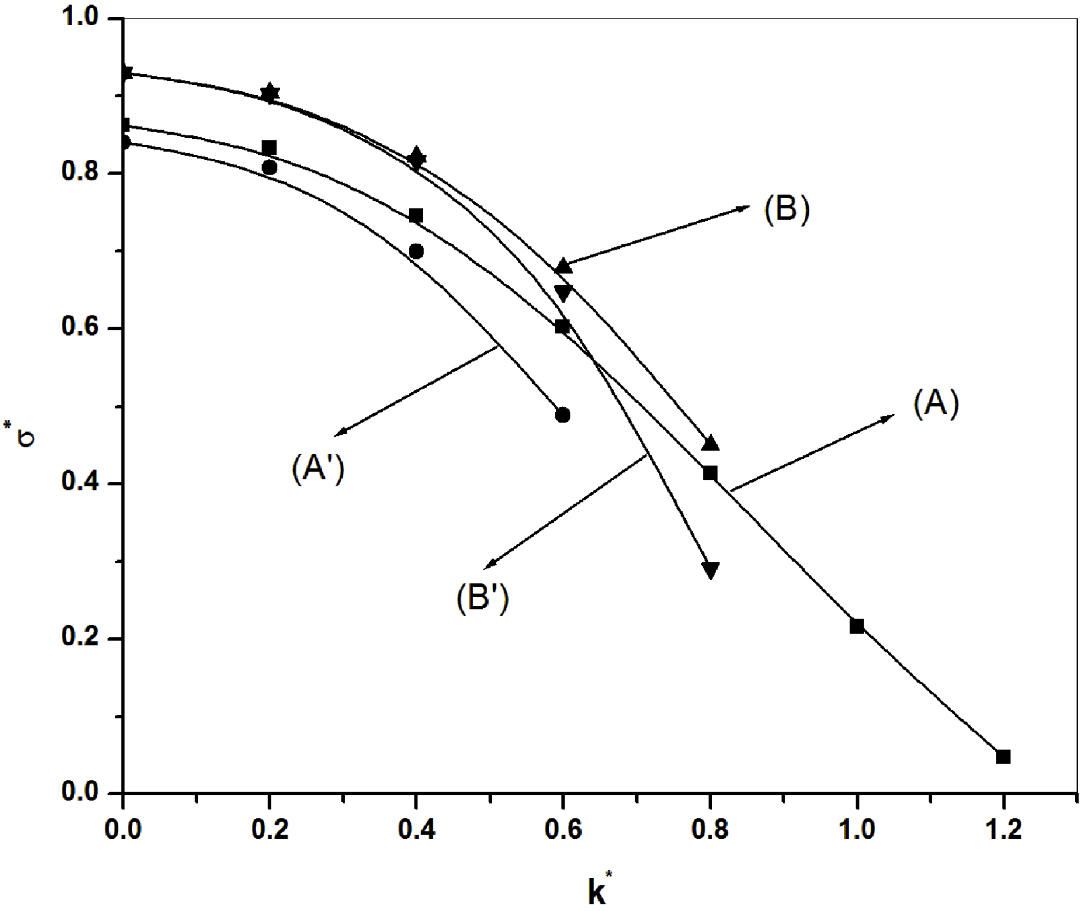
by varying one variable and keeping all other variables fixed. Figure 1 shows the comparative growth rate of the Jeans instability in the hydrodynamic and kinetic limits for both propagation regimes with the help of the normalized form of (4.3), (4.6), (4.11) and (4.14). In figure 1 the curves (A) and
 $(\text{A}^{\prime })$
are for perpendicular propagation and (B) and
 $(\text{B}^{\prime })$
are for parallel propagation for the hydrodynamic and kinetic limits, respectively. It is clear from this figure that the growth rate varies differently in the hydrodynamic regime and kinetic regimes in each direction of propagation.
The normalized growth rate
 ${\it\sigma}^{\ast }$
is plotted against the normalized wavenumber
 $k^{\ast }$
in the hydrodynamic and kinetic regimes for both directions of propagation in the case where rotation is parallel to the magnetic field.

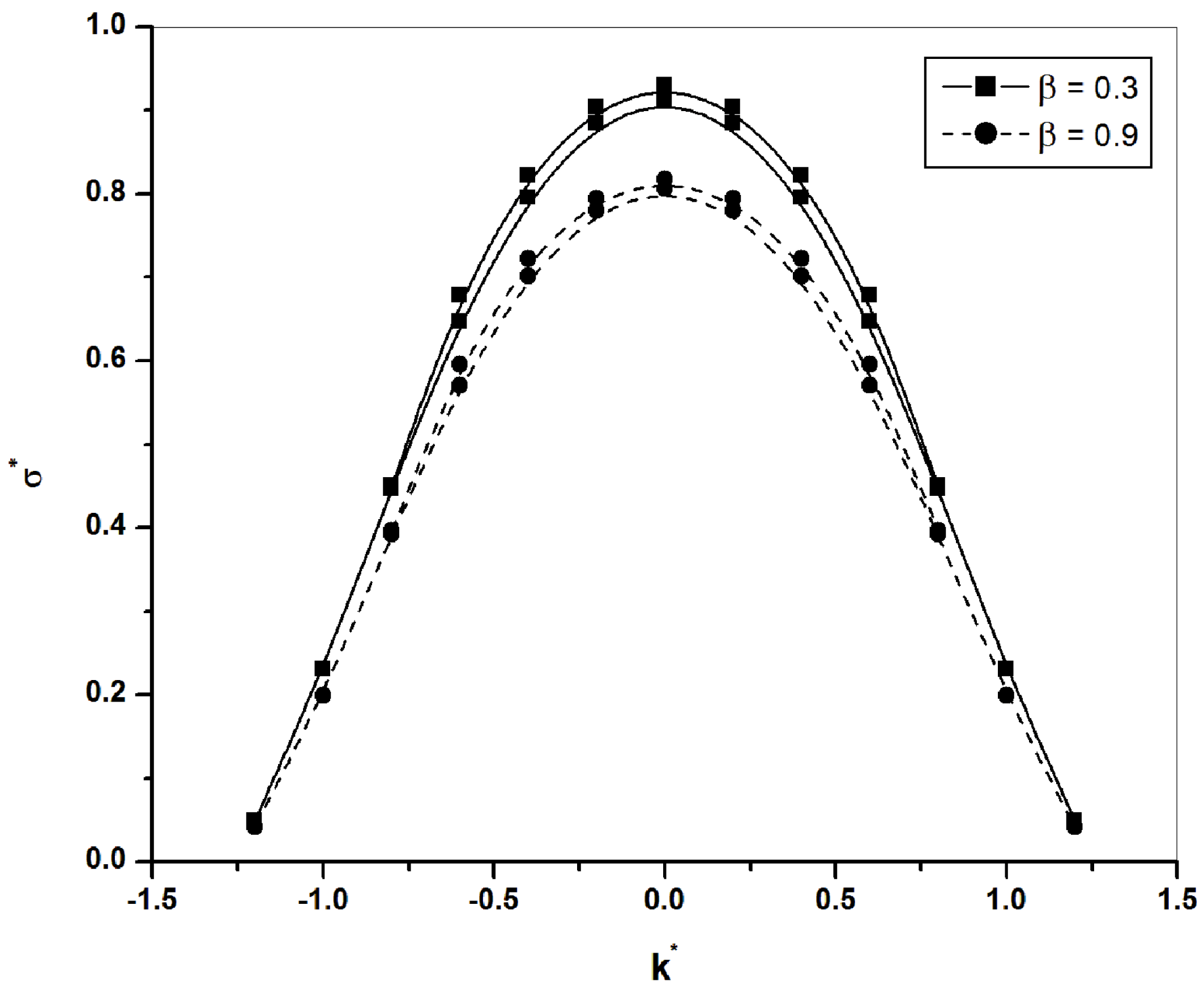
In figure 2 the growth rate of the gravitational perturbation is plotted against the wavenumber by the normalized form of (4.3) and (4.14). Figure 2 describes the effect of neutral particle to fluid density ratio in the hydrodynamic regime in the parallel and perpendicular directions of propagation. It can be clearly observed from the figure that the growth rate falls rapidly in the case of high values of
 ${\it\beta}$
and it is evident that both directions of propagation are equally affected by
 ${\it\beta}$
.
The normalized growth rate
 ${\it\sigma}^{\ast }$
is plotted against the normalized wavenumber
 $k^{\ast }$
for different values of
 ${\it\beta}$
in the hydrodynamic regime for both directions of propagation in the case when rotation is parallel to the magnetic field.

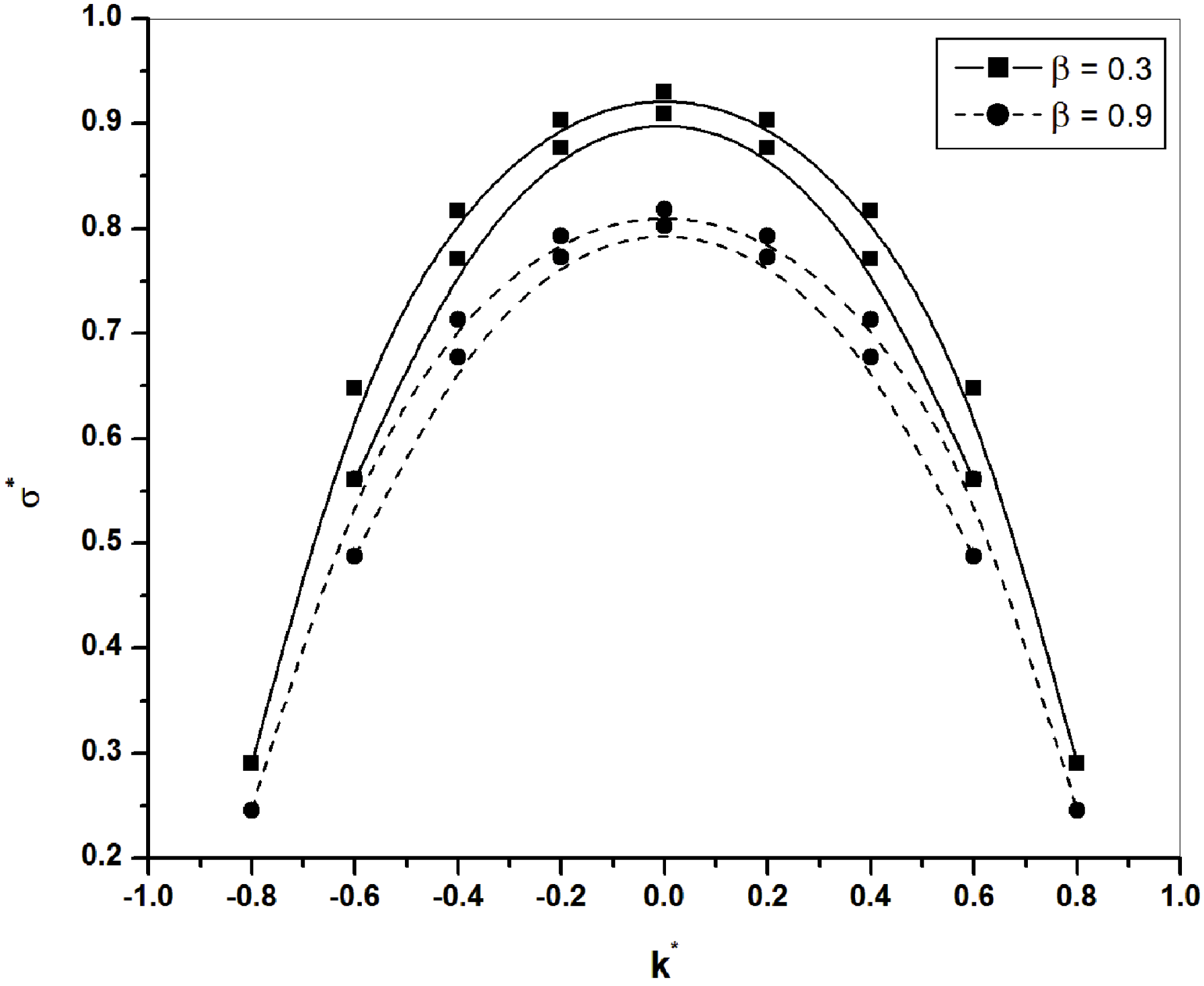
The normalized growth rate
 ${\it\sigma}^{\ast }$
is plotted against the normalized wavenumber
 $k^{\ast }$
for different values of
 ${\it\beta}$
in the kinetic regime for both directions of propagation in the case when the rotation is parallel to the magnetic field.

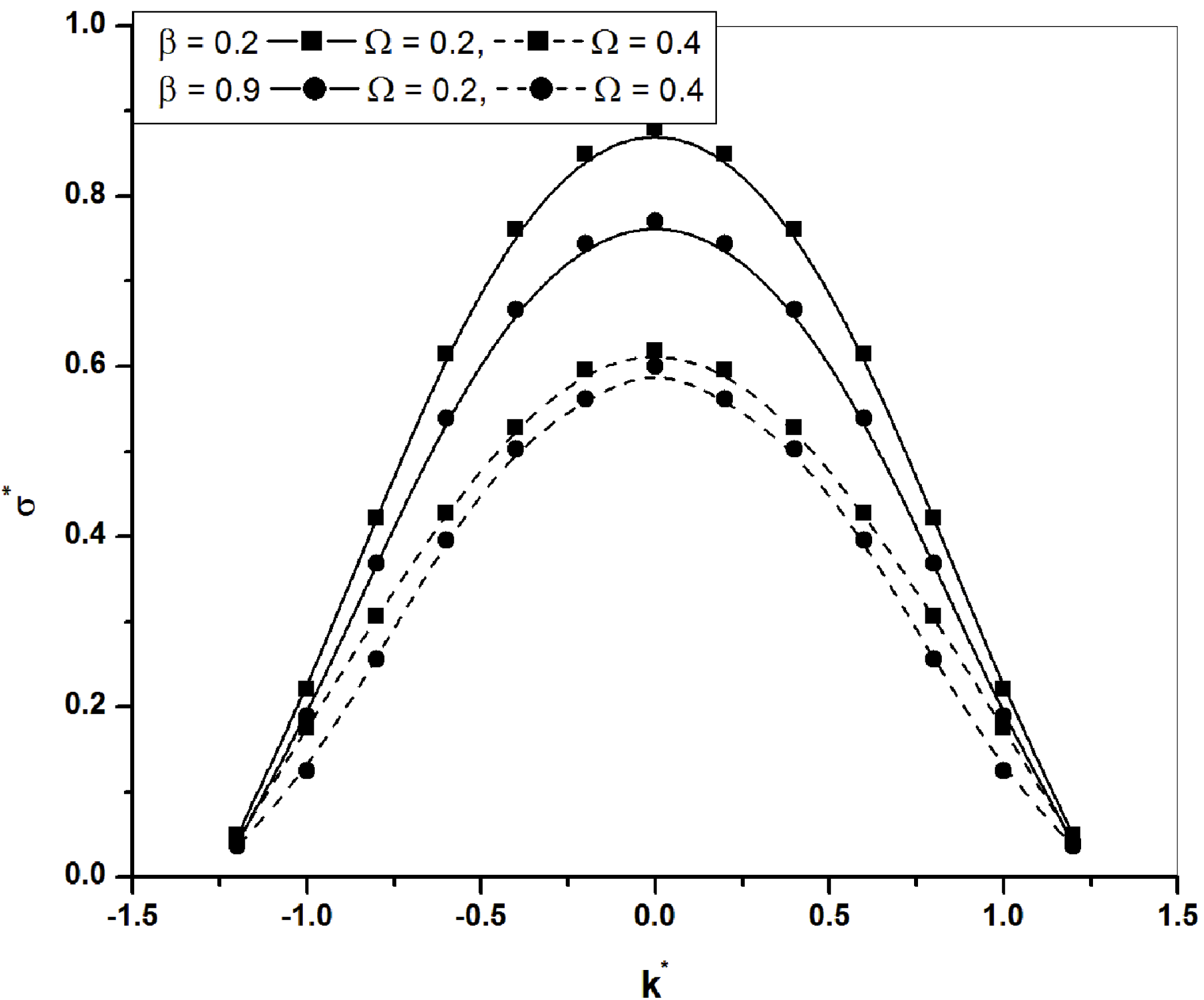
The normalized growth rate
 ${\it\sigma}^{\ast }$
is plotted against the normalized wavenumber
 $k^{\ast }$
for different rotational frequencies with variation of
 ${\it\beta}$
in the hydrodynamic regime for perpendicular propagation in the case when rotation is parallel to the magnetic field.

The normalized growth rate
 ${\it\sigma}^{\ast }$
is plotted against the normalized wavenumber
 $k^{\ast }$
for the hydrodynamic and kinetic regimes when propagation and rotation both perpendicular to the magnetic field.

Figure 3 shows a comparative study of kinetic regimes using the normalized form of (4.6) and (4.14) in the case when rotation is parallel to the magnetic field. Figure 3 shows the same observation as found in figure 2 for the kinetic regime and the effect of
 ${\it\beta}$
is the same in both kinetic and hydrodynamic regimes.
In figure 4 we have depicted the variation of growth rate with wavenumber using the normalized form of (4.6). Figure 4 shows the change of growth rate due to variation of
 ${\it\beta}$
for different rotational frequencies of the system and it is clear from the figure that the growth rate falls rapidly in the case when the rotation of the system is relatively slow.
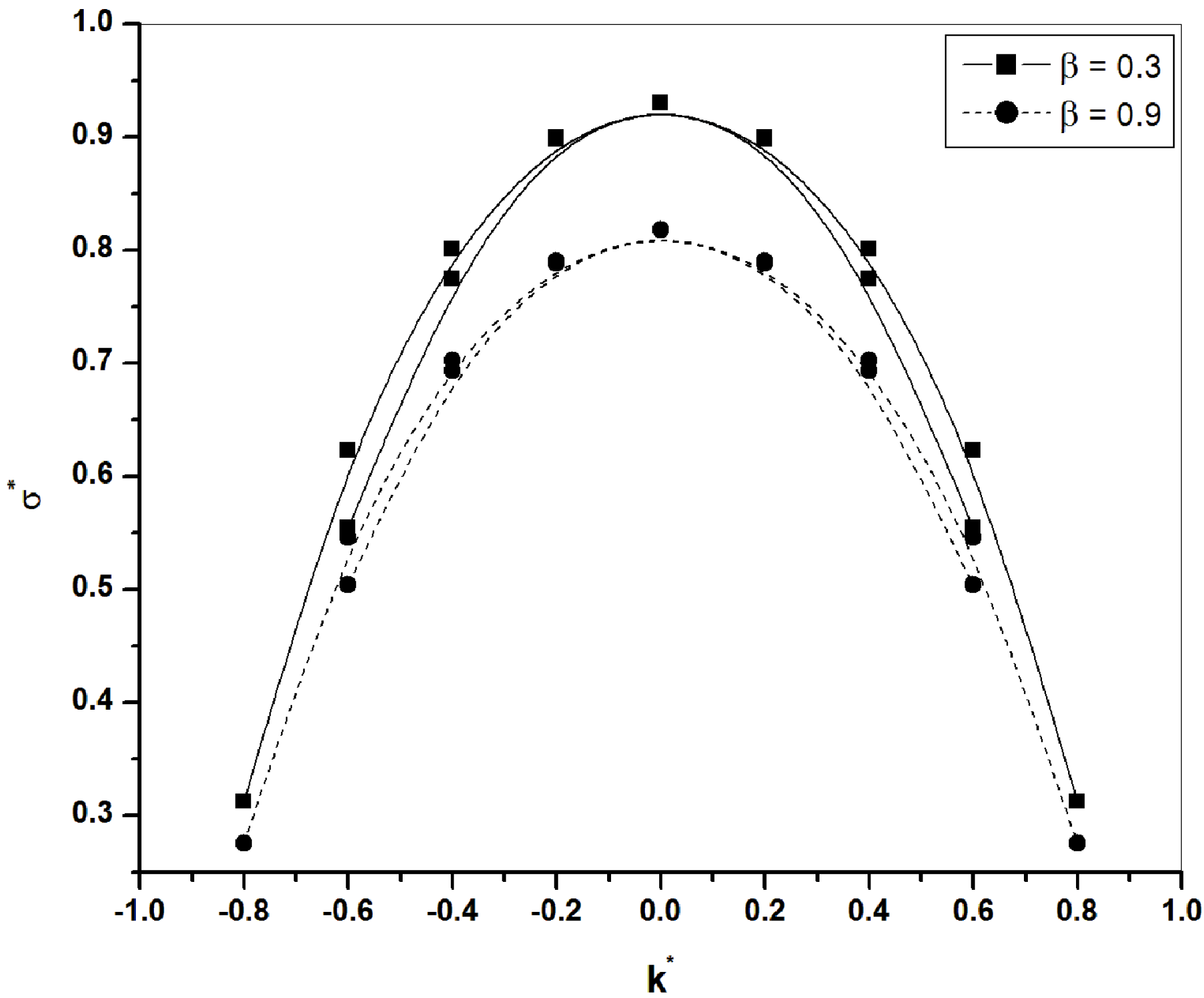
Figure 5 shows for hydrodynamic and kinetic regimes the growth rate of the Jeans instability when the axis of rotation is perpendicular to the magnetic field for different values of
 ${\it\beta}$
(using the normalized form of (4.19) and (4.22)) and it is clear from the figure that, as the value of
 ${\it\beta}$
increases, the growth rate of the gravitational perturbation decreases.
6 Conclusions
In the present work, the effects of rotation, Hall current and neutral particles on the Jeans instability of a magnetized, partially ionized, strongly coupled plasma are investigated. The dispersion relation is discussed for four different cases. Further, these cases are analysed in the hydrodynamic and kinetic limits separately. In the perpendicular propagation case, we obtain a viscous mode while in the parallel propagation case, the Alfvén mode is obtained along with the gravitational mode. It is found that all three modes are modified due to the neutral particles. The Jeans criterion of instability is studied for a gravitating mode. The influence of the Hall current on the gravitational mode is illustrated in the case of parallel propagation, when the system is rotating perpendicular to magnetic field. From the numerical interpretation it is clear that the presence of rotation and neutral particles moves the system towards stabilization.
Acknowledgements
The authors are gratefully acknowledged to SERB, New Delhi, (grant no. SB/FTP/PS – 075/2014), UGC, New Delhi, (grant no. 42-820/2013(SR)), and MPCST, Bhopal, (grant no. A/RD/RP-2/2015-16/243) for the financial support. The authors are highly thankful to Professor R. K. Chhajlani, Vikram University Ujjain (MP) for his continuous support and encouragements. The authors gratefully acknowledge the anonymous reviewer for strong suggestions to improve the work.