2.1 Navier–Stokes equations for two-dimensional flows down an incline

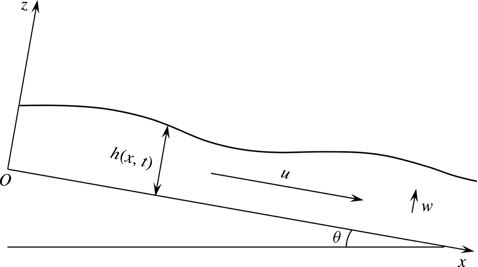
We consider a two-dimensional thin liquid, flowing down an inclined plane. The angle of the plane with respect to the horizontal is $\unicode[STIX]{x1D703}$ . The directions $Ox$ and $Oz$ are respectively the directions parallel to the plane and normal to the plane. The components of the fluid velocity field are denoted by $u$ and $w$ in the directions $Ox$ and $Oz$ respectively. The bottom wall is smooth and the fluid depth is denoted by $h$ (see figure 1).

The fluid motion is governed by the Navier–Stokes equations, completed by the boundary conditions on the bottom wall and at the free surface. The fluid is supposed to be incompressible and the capillarity is neglected. The continuity equation is

The Navier–Stokes momentum equations in the $Ox$ and $Oz$ directions are:

where $g$ is the gravitational acceleration, $p$ is the pressure and $\unicode[STIX]{x1D70F}_{xx}$ , $\unicode[STIX]{x1D70F}_{xz}$ and $\unicode[STIX]{x1D70F}_{zz}$ are the components of the viscous stress tensor $\unicode[STIX]{x1D749}$ . The boundary conditions at the bottom are the no-penetration condition and the no-slip condition

At the free surface, the kinematic boundary condition holds

and the dynamic boundary condition

The atmospheric pressure is constant and taken equal to zero.

Figure 1.

Notations used in the text.

2.2 Mixing-length model: a nonlinear constitutive law of stress tensor

The turbulence model of mixing length, initially proposed by Prandtl, is contained in the stress tensor. We denote by $\unicode[STIX]{x1D63F}$ the strain rate tensor. Instead of the classical viscous stress tensor for Newtonian fluids $\unicode[STIX]{x1D749}=2\unicode[STIX]{x1D70C}\unicode[STIX]{x1D708}\unicode[STIX]{x1D63F}$ , where $\unicode[STIX]{x1D708}$ is the kinematic viscosity, we consider the constitutive law $\unicode[STIX]{x1D749}=2\unicode[STIX]{x1D70C}(\unicode[STIX]{x1D708}+\unicode[STIX]{x1D708}_{T})\unicode[STIX]{x1D63F}$ where $\unicode[STIX]{x1D708}_{T}$ is the kinematic turbulent or eddy viscosity which depends on the $z$ variable through a function $L_{m}$ called the mixing length and on the norm of the tensor $\unicode[STIX]{x1D63F}$ , namely:

where the norm of the strain rate tensor is defined by

and the mixing length $L_{m}$ depends on the chosen model. The first one is due to Prandtl:

where $\unicode[STIX]{x1D705}$ is a dimensionless coefficient called the von Kármán constant. Its numerical value $\unicode[STIX]{x1D705}\simeq 0.4$ is obtained from experimental data. This model was later modified by Van Driest (Reference Van Driest1951, Reference Van Driest1956, Reference Van Driest and Lin1959) who added a damping term

where $A^{+}$ is also a dimensionless constant. The usual value is $A^{+}=26$ . The dimensionless variable $z^{+}$ is often referred to as a viscous, or wall, coordinate. It is defined by $z^{+}=zu_{b}/\unicode[STIX]{x1D708}$ where the shear velocity or friction velocity $u_{b}$ is related to the bottom shear stress or parietal stress $\unicode[STIX]{x1D70F}_{b}$ by $u_{b}=\sqrt{\unicode[STIX]{x1D70F}_{b}/\unicode[STIX]{x1D70C}}$ (see Henderson (Reference Henderson1996), and equation (2.32) below). We define the (kinematic) effective viscosity as the sum of the molecular viscosity and the turbulent viscosity $\unicode[STIX]{x1D708}_{eff}=\unicode[STIX]{x1D708}+\unicode[STIX]{x1D708}_{T}$ . The constitutive law can thus be written $\unicode[STIX]{x1D749}=2\unicode[STIX]{x1D70C}\unicode[STIX]{x1D708}_{eff}\unicode[STIX]{x1D63F}$ . To derive approximate one-dimensional (1-D) models, these equations are averaged over the depth. However we need two dimensionless systems in order to take into account the boundary layer near the bottom wall. Both scaling are presented next.

2.3 Shallow-water scaling

The equations are put into dimensionless form using a characteristic depth $h_{n}$ as the characteristic length in the $Oz$ direction and a characteristic speed in the $Ox$ direction $u_{n}$ . In practice, $h_{n}$ and $u_{n}$ are the depth and velocity of the uniform flow, called the normal depth and the normal velocity. The characteristic length in the $Ox$ direction is $L$ . The shallow-water hypothesis is that the aspect ratio $\unicode[STIX]{x1D700}$ is small:

The dimensionless variables in this shallow-water scaling will be denoted with a prime. They are defined by

We define further $h^{\prime }=h/h_{n}$ , the Froude number $F=u_{n}/\sqrt{gh_{n}}$ and the Reynolds number $Re=h_{n}u_{n}/\unicode[STIX]{x1D708}$ . We need a second Reynolds number related to the mixing length. The dimensionless mixing length $L_{m}^{\prime }$ can be defined by $L_{m}^{\prime }=L_{m}/(\unicode[STIX]{x1D705}h_{n})$ and the dimensionless strain rate tensor by $\unicode[STIX]{x1D63F}^{\prime }=h_{n}\unicode[STIX]{x1D63F}/u_{n}$ . The components of $\unicode[STIX]{x1D63F}^{\prime }$ can be written

so that:

The turbulent viscosity becomes $\unicode[STIX]{x1D708}_{T}=\unicode[STIX]{x1D705}^{2}h_{n}u_{n}\sqrt{2}L_{m}^{^{\prime }2}\Vert \unicode[STIX]{x1D63F}^{\prime }\Vert$ . Taking $\unicode[STIX]{x1D708}_{e}=\unicode[STIX]{x1D705}^{2}h_{n}u_{n}$ as a characteristic eddy viscosity, we can define the dimensionless turbulent viscosity as $\unicode[STIX]{x1D708}_{T}^{\prime }=\unicode[STIX]{x1D708}_{T}/\unicode[STIX]{x1D708}_{e}$ . The mixing-length Reynolds number can be defined by

Note that $Re_{ML}$ is independent of the fluid depth. Its numerical value is close to 6. It is thus much smaller that the fluid Reynolds number which is supposed to be larger than $10^{4}$ . We obtain $\unicode[STIX]{x1D708}_{T}^{\prime }=\sqrt{2}L_{m}^{\prime 2}\Vert \unicode[STIX]{x1D63F}^{\prime }\Vert$ . The dimensionless viscous stress tensor is defined as $\unicode[STIX]{x1D749}^{\prime }=\unicode[STIX]{x1D749}/(\unicode[STIX]{x1D70C}\unicode[STIX]{x1D705}^{2}u_{n}^{2})$ . This gives $\unicode[STIX]{x1D749}^{\prime }=2\,\unicode[STIX]{x1D708}_{eff}^{\prime }\unicode[STIX]{x1D63F}^{\prime }$ with $\unicode[STIX]{x1D708}_{eff}^{\prime }=\unicode[STIX]{x1D708}_{T}^{\prime }+\unicode[STIX]{x1D708}/\unicode[STIX]{x1D708}_{e}$ . The ratio

is an important quantity. It can also be written $\unicode[STIX]{x1D702}=\unicode[STIX]{x1D708}/\unicode[STIX]{x1D708}_{e}$ . Usual values of $\unicode[STIX]{x1D702}$ lie in the range $10^{-4}$ – $10^{-6}$ . A typical value of $\unicode[STIX]{x1D700}$ being $10^{-2}$ , we can assume that $\unicode[STIX]{x1D702}<\unicode[STIX]{x1D700}$ . In many cases, we have also $\unicode[STIX]{x1D702}<\unicode[STIX]{x1D700}^{2}$ and this will be our choice. In the following, we will suppose that

The grounds for this choice are explained in § 3.2. The dimensionless effective viscosity can be written

The expression of the dimensionless mixing length can be simplified as

and the effective viscosity becomes

With this scaling, the continuity equation (2.1) becomes simply

The momentum equation in the $Oz$ direction (2.3) can be written

This means that the pressure is hydrostatic at this approximation. In this scaling, $\sin \unicode[STIX]{x1D703}$ is $O(1)$ . Denoting

the momentum equation in the $Ox$ direction (2.2) becomes

Another assumption for this model is that $\unicode[STIX]{x1D700}/(\unicode[STIX]{x1D705}^{2}F^{2})=O(\unicode[STIX]{x1D700})$ . This implies that $F=O(1)$ . The no-penetration and no-slip conditions are simply $w^{\prime }(0)=0$ and $u^{\prime }(0)=0$ . Likewise the kinematic boundary condition at the free surface is the same as (2.5) but with dimensionless quantities (with a prime symbol). The dynamic boundary conditions at the free surface can be written

However, the above scaling is not sufficient to provide a consistent description of the flow. In particular, this scaling leads to a singular expansion in the asymptotic regime we are interested in. Even at order zero, we cannot reach the Dirichlet boundary condition at the bottom. This lack of consistency with the physical boundary condition comes from the presence of the dimensionless parameter $\unicode[STIX]{x1D702}$ which is very small in our asymptotic regime. Consequently, it is natural to introduce another scaling, called the viscous scaling, which is presented below.

2.4 Viscous scaling

This scaling is made in order to get suitable bounds of $u$ , $w$ , $\unicode[STIX]{x1D70F}_{xz}$ and $\unicode[STIX]{x1D70F}_{xx}$ , together with their time and spatial derivatives. Above all, this second scaling, only used near the bottom wall, allows us to recover consistency with boundary conditions (2.4). Actually, it consists in a zoom of the previous system close to the wall. This zoom is naturally done using the parameter $\unicode[STIX]{x1D702}$ . We define dimensionless quantities in the viscous scaling, denoted with a tilde symbol. Some are the same as in the first scaling,

while others are magnified,

We thus obtain the following viscous dimensionless mass and momentum balances:

together with the boundary conditions $\tilde{w}(0)=0$ , $\tilde{u} (0)=0$ , $\tilde{w}(h)=\unicode[STIX]{x2202}\tilde{h}/\unicode[STIX]{x2202}\tilde{t}+\tilde{u} (h)\unicode[STIX]{x2202}\tilde{h}/\unicode[STIX]{x2202}\tilde{x}$ , $\tilde{p}(h)=O(\unicode[STIX]{x1D700})$ and $\tilde{\unicode[STIX]{x1D70F}}_{xz}(h)=O(\unicode[STIX]{x1D700}^{2})$ . Note that our new variables are related to the classical viscous variables (see for example Henderson Reference Henderson1996; Sturm Reference Sturm2010):

Moreover, in this scaling, the dimensionless mixing length is magnified as $\tilde{L}_{m}=L_{m}^{\prime }/\unicode[STIX]{x1D702}$ , so that

while the strain rate tensor is $\tilde{\unicode[STIX]{x1D63F}}=\unicode[STIX]{x1D702}\unicode[STIX]{x1D63F}^{\prime }$ . The effective viscosity becomes

with

3.1 General methodology

The asymptotic expansions of the solution to the dimensionless Navier–Stokes equations are built with an iterative algorithm, consisting in resolving a differential system at each order with respect to the small parameter $\unicode[STIX]{x1D700}$ . This method is formally the same as the method proposed in Noble & Vila (Reference Noble and Vila2013) for power-law laminar flows and in Richard et al. (Reference Richard, Ruyer-Quil and Vila2016) for laminar Newtonian flows. It is a little bit more tedious in the present case because of the singularity of the expansions. The formal Hilbert expansions of the solutions

are put into the dimensionless Navier–Stokes equations in the shallow-water scaling. Since the resolution of this system at a given order gives some expressions that diverge when $z\rightarrow 0$ , the same kind of expansions and computations will be done for the viscous system. For instance, the asymptotic expansion of $\tilde{u}$ will be $\tilde{u} =\tilde{u} _{0}+\unicode[STIX]{x1D700}\tilde{u} _{1}+O(\unicode[STIX]{x1D700}^{2})$ . The expressions obtained for the viscous system are valid in an internal layer (close to the bottom), whereas those obtained for the shallow-water scaling are valid in the external layer (above the internal layer). For $Re\gg 1$ , or equivalently $\unicode[STIX]{x1D702}\ll 1$ , the internal layer is very thin, hence the zoom $\tilde{z}=z^{\prime }/\unicode[STIX]{x1D702}$ . We assume the existence of a buffer layer or overlap domain at a depth $z/h=O(\sqrt{\unicode[STIX]{x1D702}})$ . To get a consistent expansion, a matching procedure is used (see Cousteix & Mauss Reference Cousteix and Mauss2007, for example): both expressions must fit in the overlap domain defined by $\sqrt{\unicode[STIX]{x1D702}}\,b_{1}h<z<\sqrt{\unicode[STIX]{x1D702}}\,b_{2}h$ where $b_{1}$ and $b_{2}$ are two positive dimensionless numbers of $O(1)$ . The assumption of such an overlap layer leads to a consistent model of order 1 with the proviso that (2.17) is satisfied (see § 3.2 and (3.15) below).

The different stages of the computations at each order are the following: first, $\unicode[STIX]{x1D70F}_{xz}$ is obtained by the vertical integration of the momentum equation in the $Ox$ direction; then $\unicode[STIX]{x2202}u/\unicode[STIX]{x2202}z$ is built thanks to the constitutive law; we can then reconstruct $u$ by integration; the mass equation allows us to calculate the vertical velocity $w$ ; finally, the pressure $p$ is obtained by the vertical integration of the momentum equation in the $Oz$ direction. Once the algorithm is done at order $k$ , we repeat the procedure at order $k+1$ . In practice, the computations will be done only at order zero and order 1 (the computation at order 2 would add the computation of $\unicode[STIX]{x1D70F}_{xx}=-\unicode[STIX]{x1D70F}_{zz}$ ).

3.2 Order zero

At order zero, equation (2.24) reduces to $\unicode[STIX]{x2202}\unicode[STIX]{x1D70F}_{0}^{\prime }/\unicode[STIX]{x2202}z^{\prime }=-\unicode[STIX]{x1D706}$ . Since $\unicode[STIX]{x1D70F}_{xz}^{\prime }(h)=O(\unicode[STIX]{x1D700}^{2})$ (equation (2.26)), the integration leads to

The constitutive law and the expression of the effective viscosity (2.20) give

Defining $s=z^{\prime }/h^{\prime }$ , the inversion of this relation leads to

The velocity $u_{0}^{\prime }$ is obtained by integration

where the function $j$ is defined by

and where $u_{0}^{\prime }(h^{\prime })$ is the velocity at the free surface ( $s=1$ ). The examination of the expressions of $\unicode[STIX]{x1D70F}_{0}$ and $u_{0}^{\prime }$ shows that, when $z^{\prime }\rightarrow 0$ , $\unicode[STIX]{x1D70F}_{0}\rightarrow \unicode[STIX]{x1D706}h^{\prime }$ whereas $u_{0}^{\prime }$ diverges. The matching procedure is needed to find the complete expression of $u_{0}^{\prime }$ (in particular the value of $u_{0}^{\prime }(h^{\prime })$ ).

In the viscous layer, equation (2.30) implies that $\tilde{\unicode[STIX]{x1D70F}}_{0}$ is constant. The matching procedure for $\unicode[STIX]{x1D70F}_{0}^{\prime }$ is then straightforward:

The constitutive law, together with the expression (2.34) of the effective viscosity gives

This equation is inverted by solving a second-order algebraic equation. It yields

where $\unicode[STIX]{x1D709}=2\sqrt{\unicode[STIX]{x1D706}h^{\prime }}\tilde{z}$ and $A=2\unicode[STIX]{x1D705}A^{+}$ . By integration, with the no-slip condition $\tilde{u} _{0}(0)=0$ , we find

where the function ${\mathcal{R}}$ is defined by

This function has a finite limit when $\unicode[STIX]{x1D709}\rightarrow \infty$ which will be denoted by $R$ . The expression (3.8) in the external layer and the expression (3.13) in the internal layer are now fitted by the matching procedure: we solve $u_{0}^{\prime }(z=\sqrt{\unicode[STIX]{x1D702}}\,bh)=\tilde{u} _{0}(z=\sqrt{\unicode[STIX]{x1D702}}\,bh)+O(\sqrt{\unicode[STIX]{x1D702}})$ , with $0<b_{1}<b<b_{2}$ . It is possible provided that

where the function $M$ is given by $M=2\sqrt{\unicode[STIX]{x1D706}h^{\prime 3}}$ . The term $O(\sqrt{\unicode[STIX]{x1D702}})$ has to be asymptotically smaller than $\unicode[STIX]{x1D700}$ in order to get consistency at order 1, hence the choice (2.17). There appears a term of $O(-\ln \unicode[STIX]{x1D702})$ . Let

Thereafter, this parameter will be treated as a small parameter satisfying the condition:

The significance of this point will be highlighted later in this paper (see § 4.3). By definition, the small parameter $\unicode[STIX]{x1D707}$ depends on $\unicode[STIX]{x1D700}$ as

where $m$ is defined in (2.17). Since

the main small parameter $\unicode[STIX]{x1D700}$ is smaller than $\unicode[STIX]{x1D707}^{p}$ for any positive integer $p$ if $\unicode[STIX]{x1D700}$ is small enough. Each term of the asymptotic expansions of a given order, such as $u_{1}^{\prime }$ , is further expanded in a power series of this second small parameter $\unicode[STIX]{x1D707}$ .

The expression (3.15) shows that $u_{0}^{\prime }(h^{\prime })$ is of $O(\sqrt{\unicode[STIX]{x1D706}}/\unicode[STIX]{x1D707})$ . As we want $u_{0}^{\prime }$ to be of $O(1)$ , this implies that $\unicode[STIX]{x1D706}=O(\unicode[STIX]{x1D707}^{2})$ . We thus assume

where $\unicode[STIX]{x1D706}_{0}=O(1)$ . Then $M=2\unicode[STIX]{x1D707}\sqrt{\unicode[STIX]{x1D706}_{0}h^{\prime 3}}$ , and the free surface velocity (3.15) becomes

Note that practically $\ln \unicode[STIX]{x1D707}=O(1)$ . For instance, if $\unicode[STIX]{x1D702}\sim 10^{-4}$ , $\ln \unicode[STIX]{x1D707}\sim -1.5$ . Hence $\ln M=O(1)$ . The complete expression of $u_{0}^{\prime }$ is finally

Even if neither $u_{0}^{\prime }$ nor $\tilde{u} _{0}$ are valid approximations of the velocity on the whole fluid depth, we can use any of them to compute an average velocity since they are integrable functions on $[0,h]$ and that the values of these integrals match up to a small error with respect to $\unicode[STIX]{x1D700}$ . The average value over the fluid depth of any quantity $X$ being defined by

it is natural to compute the average velocity from the expression (3.22). Writing $U=\langle u\rangle$ , this gives

The vertical velocity is computed from the continuity equation. Taking into account the kinematic boundary condition at the free surface, the integration of (2.21) leads to

To estimate the derivative of $h^{\prime }$ with respect to $t^{\prime }$ , the continuity equation is averaged over the depth. Thanks to the no-penetration boundary condition, we get

Consequently, $\unicode[STIX]{x2202}h^{\prime }/\unicode[STIX]{x2202}t^{\prime }$ can be estimated by

where $U_{0}^{\prime }$ is given by (3.24). At order zero, the vertical velocity is found by

where $s=z^{\prime }/h^{\prime }$ . The result of the calculation is

Finally, the zeroth-order pressure is computed readily from (2.22):

Equation (2.31) implies that $\tilde{p}_{0}$ is constant in the internal layer. Connecting this constant by the usual matching procedure gives simply $\tilde{p}_{0}=h^{\prime }\cos \unicode[STIX]{x1D703}$ .

3.3 Order 1

At order 1, the momentum equation in the $Ox$ direction (2.24) is

Making use of the boundary condition at the free surface, integration of (3.31) gives:

The valued of $\unicode[STIX]{x2202}h^{\prime }/\unicode[STIX]{x2202}t$ is estimated with (3.27). A long calculation yields

where $s=z^{\prime }/h^{\prime }$ and:

It appears that $\unicode[STIX]{x1D70F}_{1}^{\prime }$ possesses a finite limit when $z^{\prime }\rightarrow 0$ (or $s\rightarrow 0$ ), namely

with

In the internal (viscous) layer, equation (2.30) implies that $\tilde{\unicode[STIX]{x1D70F}}_{1}$ is constant. It follows from the matching procedure that this constant is equal to $\unicode[STIX]{x1D70F}_{1}^{\prime }(0)$ given by equation (3.35).

Next, the constitutive law and the external (shallow-water) effective viscosity (2.20) give

The inversion of this relation gives

The expression of the velocity at order 1 in the external layer is found by integration:

Because $u_{1}^{\prime }$ diverges when $s\rightarrow 0$ , we proceed as for the zeroth order: the same calculation is done in the internal layer and both expressions are fitted in the overlap domain. With the constitutive law and the internal effective viscosity (2.34), we get

Since $\tilde{\unicode[STIX]{x1D70F}}_{1}$ is constant and equal to $\unicode[STIX]{x1D70F}_{1}^{\prime }(0)$ ,

where $\unicode[STIX]{x1D709}=2\sqrt{\unicode[STIX]{x1D706}h^{\prime }}\tilde{z}$ and $A=2\unicode[STIX]{x1D705}A^{+}$ . Integrating this expression from 0 to $\unicode[STIX]{x1D709}$ , taking into account the no-slip condition, we find

where the function ${\mathcal{R}}_{1}$ is defined by

This function possesses a finite limit when $\unicode[STIX]{x1D709}\rightarrow \infty$ which will be denoted by $R_{1}$ . The replacement of ${\mathcal{R}}_{1}(Mb/\sqrt{\unicode[STIX]{x1D702}})$ by $R_{1}$ in the matching procedure below is justified in a similar way as for $R$ (see appendix A).

To match the external velocity with the inner one, we solve, for $0<b_{1}<b<b_{2}$ ,

A very long calculation yields

where

The final expression of $u_{1}^{\prime }$ is

Even if this expression is not valid over the whole fluid depth (it diverges for $z\rightarrow 0$ ) and must be connected to the inner expression, $u_{1}^{\prime }$ possesses a finite average value over the whole depth. This first-order average velocity, denoted by $U_{1}^{\prime }=\langle u_{1}^{\prime }\rangle$ is given by:

We are now able to derive our reduced models of smooth turbulent free surface flow.

4.1 Averaged equations

Models are obtained from an averaging procedure over the fluid depth (see (3.23)) of the Navier–Stokes equations, taking into account the boundary conditions and the formal asymptotic expansions of § 3. An advantage of this approach is that the dimensionality of the model is one less than for the starting equations and that the boundary conditions are incorporated into the equations of the model. As a consequence, the numerical resolution is much faster and easier provided that the equations of the model have an appropriate mathematical structure.

The equations are averaged in the shallow-water scaling. We recall that we denote by $U^{\prime }=\langle u^{\prime }\rangle$ the average fluid velocity. The averaging of the continuity equation (2.21) was done above (equation (3.26)): note that it is exact. Next, let us average the momentum equation in the $Ox$ -direction (2.24). At the first order of approximation, the pressure is hydrostatic (see (3.30)), so that we obtain

The average quantity $\langle u^{\prime 2}\rangle$ is expressed by decomposing the velocity as the sum of its average value and a deviation $u^{\ast }$ to this average value:

This method will be proved to be very similar to that used by Teshukov (Reference Teshukov2007). In particular, it will be shown below that the introduction of the small parameter $\unicode[STIX]{x1D707}$ in (3.16) is equivalent to Teshukov’s approximation of weakly sheared flows (Teshukov Reference Teshukov2007). Equation (4.1) becomes

To handle $\langle u^{\ast 2}\rangle$ , a third variable called enstrophy is introduced as in Richard & Gavrilyuk (Reference Richard and Gavrilyuk2012) and Richard et al. (Reference Richard, Ruyer-Quil and Vila2016). The enstrophy is defined as

One of the advantage of the enstrophy is that it acts as the mathematical entropy of the hyperbolic model (Richard & Gavrilyuk Reference Richard and Gavrilyuk2012). The momentum equation becomes

Since there are now three unknowns in the model, a third equation is needed to close the system. This equation is provided by the work-energy theorem also called theorem of the kinetic energy. In the present case, and in the shallow-water scaling, it reads

where the colon symbol denotes the double contraction. More explanations can be found in Richard et al. (Reference Richard, Ruyer-Quil and Vila2016). Averaging this equation over the depth, we get

where $W^{\prime }$ is the dimensionless power dissipated inside the flow by effective viscous effects

Up to now, we obtained a set of three equations: the mass equation (3.26), the momentum equation (4.5) and the energy equation (4.7). Note that $\langle u^{\ast 3}\rangle$ appears in the latter. But we will see below that it is possible to get rid of it and thus to close the problem.

4.2 Asymptotic expansion of the enstrophy and of $\langle u^{\ast 3}\rangle$

Since the enstrophy is a variable of the system, its asymptotic expansion is needed to build the model. We write $\unicode[STIX]{x1D711}^{\prime }=\unicode[STIX]{x1D711}_{0}^{\prime }+\unicode[STIX]{x1D700}\unicode[STIX]{x1D711}_{1}^{\prime }+O(\unicode[STIX]{x1D700}^{2})$ . Likewise, the velocity deviation is expanded as $u^{\ast }=u_{0}^{\ast }+\unicode[STIX]{x1D700}u_{1}^{\ast }+O(\unicode[STIX]{x1D700}^{2})$ with $u_{0}^{\ast }=u_{0}^{\prime }-U_{0}^{\prime }$ and $u_{1}^{\ast }=u_{1}^{\prime }-U_{1}^{\prime }$ . At order zero, the enstrophy is calculated by $\unicode[STIX]{x1D711}_{0}^{\prime }=\langle u_{0}^{\ast 2}\rangle /h^{\prime 2}$ :

The expression of the enstrophy at order 1, computed from $\unicode[STIX]{x1D711}_{1}^{\prime }=2\langle u_{0}^{\ast }u_{1}^{\ast }\rangle /h^{\prime 2}$ , is

The asymptotic expansion at order zero of $\langle u^{\ast 3}\rangle$ is

4.3 Weakly sheared flows

The asymptotic expansion at order zero of the velocity deviation is

where $s=z^{\prime }/h^{\prime }$ . This expression shows that $u_{0}^{\ast }=O(\unicode[STIX]{x1D707})$ . From the expression (4.9), we have $\unicode[STIX]{x1D711}_{0}^{\prime }=O(\unicode[STIX]{x1D707}^{2})$ and from (4.11), $\langle u_{0}^{\ast 3}\rangle =O(\unicode[STIX]{x1D707}^{3})$ . Consequently, these quantities are small since $\unicode[STIX]{x1D707}$ is a small parameter. The deviation of the velocity from its average value is small and this implies that the flow is weakly sheared. Teshukov formulated the approximation of weakly sheared flows by stating that the deviation of the velocity from its average value was of $O(\unicode[STIX]{x1D700}^{\unicode[STIX]{x1D6FD}})$ where $0<\unicode[STIX]{x1D6FD}<1$ (Teshukov Reference Teshukov2007). Our approach allows us to recover Teshukov’s approximation with $\unicode[STIX]{x1D707}$ replacing $\unicode[STIX]{x1D700}^{\unicode[STIX]{x1D6FD}}$ . Recall that $\unicode[STIX]{x1D707}$ is defined by (3.16), and satisfies (3.17). The condition $0<\unicode[STIX]{x1D6FD}<1$ is equivalent to $\unicode[STIX]{x1D700}<\unicode[STIX]{x1D707}<1$ . For typical values of the Reynolds number in turbulent open-channel flows, i.e. $10^{4}<Re<10^{7}$ , the parameter $\unicode[STIX]{x1D702}$ lies in the range $6\times 10^{-7}$ – $6\times 10^{-4}$ . We have then $0.14<\unicode[STIX]{x1D707}<0.27$ and also $2.0\times 10^{-2}<\unicode[STIX]{x1D707}^{2}<7.3\times 10^{-2}$ and $2.7\times 10^{-3}<\unicode[STIX]{x1D707}^{3}<2.0\times 10^{-2}$ . The parameter $\unicode[STIX]{x1D707}$ is not independent of the small parameter $\unicode[STIX]{x1D700}$ (see (3.18)) and $\unicode[STIX]{x1D700}$ is smaller than $\unicode[STIX]{x1D707}^{p}$ for any positive integer $p$ if $\unicode[STIX]{x1D700}$ is small enough (see (3.19)). In practice, $\unicode[STIX]{x1D700}$ has a small but finite value. The condition $\unicode[STIX]{x1D700}<\unicode[STIX]{x1D707}<1$ is satisfied for usual values of $\unicode[STIX]{x1D700}$ ( ${\sim}10^{-2}$ ) and $Re$ . Further, the condition $\unicode[STIX]{x1D700}<\unicode[STIX]{x1D707}^{2}$ can be acceptable. 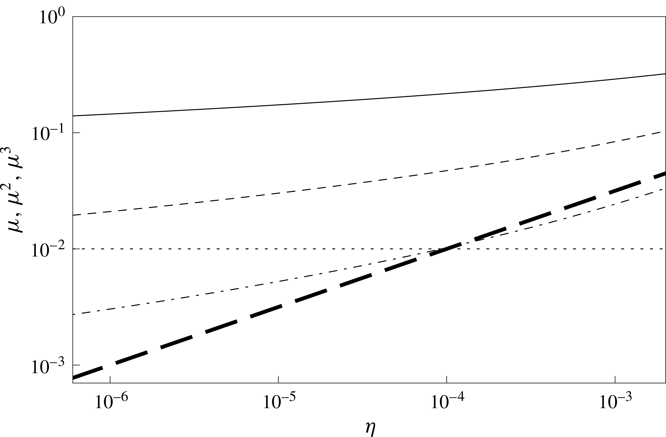On the other hand, $\unicode[STIX]{x1D707}^{3}$ is greater than $\unicode[STIX]{x1D700}$ only for very small values of $\unicode[STIX]{x1D700}$ and $\unicode[STIX]{x1D702}$ (see in figure 2 the graphs of $\unicode[STIX]{x1D707}$ , $\unicode[STIX]{x1D707}^{2}$ and $\unicode[STIX]{x1D707}^{3}$ as functions of $\unicode[STIX]{x1D702}$ ). We can thus reasonably neglect terms of $O(\unicode[STIX]{x1D707}^{3})$ . Note that the asymptotic expansion is valid if $\unicode[STIX]{x1D700}>\sqrt{\unicode[STIX]{x1D702}}$ . More precisely $\unicode[STIX]{x1D702}=\unicode[STIX]{x1D700}^{2+m},m>0$ (see (2.17)).

Figure 2.

Values of $\unicode[STIX]{x1D707}$ (solid curve), $\unicode[STIX]{x1D707}^{2}$ (dashed curve) and $\unicode[STIX]{x1D707}^{3}$ (dot-dashed curve) as functions of $\unicode[STIX]{x1D702}$ . The typical value $\unicode[STIX]{x1D700}=10^{-2}$ is shown (dotted line). The thick dashed curve is $\sqrt{\unicode[STIX]{x1D702}}$ , which is the minimum value of $\unicode[STIX]{x1D700}$ for the model to be consistent.

A similar approximation was used by Luchini & Charru (Reference Luchini and Charru2010b ) who introduced, after Mellor (Reference Mellor1972), the small parameter $u_{b}/U$ which is approximately proportional to $\ln ^{-1}(Re_{b})$ where $Re_{b}=hu_{b}/\unicode[STIX]{x1D708}$ . The deviation of the velocity from its average value was taken into account by terms who were found to be of the order of $(u_{b}/U)^{2}$ while terms of the order of $(u_{b}/U)^{3}$ were neglected. The small parameter $u_{b}/U$ plays the same role as our parameter $\unicode[STIX]{x1D707}$ which can be written $\unicode[STIX]{x1D707}=2\ln ^{-1}(\unicode[STIX]{x1D705}^{2}Re)$ .

Teshukov’s approximation of weakly sheared flows allows us to neglect, in the energy equation, the term in $\langle u^{\ast 3}\rangle$ , which is of $O(\unicode[STIX]{x1D700}^{3\unicode[STIX]{x1D6FD}})$ (see Teshukov (Reference Teshukov2007) for the general two-dimensional case or Richard & Gavrilyuk (Reference Richard and Gavrilyuk2012) for the 1-D case). This is equivalent to neglect terms of $O(\unicode[STIX]{x1D707}^{3})$ in our equations. Therefore we will neglect all terms of $O(\unicode[STIX]{x1D707}^{3})$ and in particular, the term $\langle u^{\ast 3}\rangle$ . On the other hand, the terms with the enstrophy, which are of $O(\unicode[STIX]{x1D707}^{2})$ in our approach or of $O(\unicode[STIX]{x1D700}^{2\unicode[STIX]{x1D6FD}})$ in Teshukov’s approach, can be kept since, in practice, $\unicode[STIX]{x1D700}$ can be smaller than $\unicode[STIX]{x1D707}^{2}$ . The momentum equation (4.5) becomes

and the energy equation (4.7)

where

Note that the left-hand side of system (4.13)–(4.14), together with (3.26), is analogous to the compressible Euler equations, with $P^{\prime }$ the pressure and $e^{\prime }$ the energy, the term $h^{\prime 2}\unicode[STIX]{x1D711}^{\prime }/2+h^{\prime }\cos \unicode[STIX]{x1D703}/(2F^{2})$ being the analogous of the internal energy (see Teshukov (Reference Teshukov2007) and Richard & Gavrilyuk (Reference Richard and Gavrilyuk2012) for more explanations on this analogy).

4.4 Asymptotic expansion of the dissipation power $W$

The dissipation power $W^{\prime }$ is expanded as $W^{\prime }=W_{0}^{\prime }+\unicode[STIX]{x1D700}W_{1}^{\prime }+O(\unicode[STIX]{x1D700}^{2})$ . Contrary to the integral of the velocity, the integral from $0$ to $h^{\prime }$ of $\unicode[STIX]{x1D749}^{\prime }:\unicode[STIX]{x1D63F}^{\prime }$ , as expressed with the external expansion, diverges. To calculate $W$ at any order, this integral should be divided into two parts, from the bottom to the overlap domain with the internal expansion and from the overlap domain to the free surface with the external expansion. The result depends on the exact position of the junction between the two parts. Consequently, the direct calculation of this integral is not possible. Because there is not a single regular expansion from the bottom to the free surface, the first-order correction of the dissipation power $W$ is not equal to zero and has to be calculated. Fortunately, the integral of the other terms of the energy equation, with the external expansion, does not diverge and can be used to calculate the dissipation power. At order zero, we get $W_{0}^{\prime }=\unicode[STIX]{x1D706}h^{\prime }U_{0}^{\prime }$ , or

The expression of $W_{1}^{\prime }$ is found with

The result of this calculation is

where

It is important to note that, in the general case, $W^{\prime }\neq \unicode[STIX]{x1D70F}^{\prime }(0)U^{\prime }$ . At the order zero in $\unicode[STIX]{x1D707}$ , we have $W_{0}^{\prime }=\unicode[STIX]{x1D70F}_{0}^{\prime }(0)U_{0}^{\prime }$ , but at the order $O(\unicode[STIX]{x1D707}^{2})$ , we get instead

This means that, if the shearing cannot be neglected i.e. at the order $O(\unicode[STIX]{x1D707}^{2})$ , which is the order of magnitude of the enstrophy, then the energy dissipation power is not the power of the friction force which appears in the averaged momentum equation. The difference between the momentum equation and the energy equation was clearly explained by several authors (Chow Reference Chow1959, p. 51; Yen Reference Yen1973, Reference Yen2002): the averaged momentum equation involves only the forces external to the flow (in the present case the friction on the bottom wall). On the other hand, the energy equation, derived from the work-energy theorem includes the power of both the external and internal forces. Because of the no-slip condition, the friction force at the bottom does not do work. The dissipation power thus encompasses only the power dissipated by the viscous forces, which are internal to the flow. Consequently, the dissipation power in the averaged energy equation has no reason to be always equal to the product of the bottom friction force and of the averaged velocity. The equality is true in the particular case of a negligible shearing, i.e. when the velocity is almost constant over the depth. In the case of a uniform flow, $\unicode[STIX]{x2202}h^{\prime }/\unicode[STIX]{x2202}x^{\prime }=0$ and $W^{\prime }=\unicode[STIX]{x1D70F}_{xz}^{\prime }(0)U^{\prime }+O(\unicode[STIX]{x1D700}\unicode[STIX]{x1D707}^{3})$ . This is also approximately the case if the flow is very gradually varied, i.e. when $|\unicode[STIX]{x2202}h^{\prime }/\unicode[STIX]{x2202}x^{\prime }|\ll 1$ . Then the energy equation would be redundant, since it can be deduced from the mass and momentum equations. But when the shearing is not negligible, the averaged energy equation becomes independent of the averaged momentum equation. A third variable is necessary to take into account the shearing effect, for example the enstrophy (4.4), and the averaged energy equation provides the third equation needed to close the problem.

4.5 Saint-Venant model

The Saint-Venant model (Barré de Saint-Venant Reference Barré de Saint-Venant1871) is an approximation of order $1$ with respect to $\unicode[STIX]{x1D700}$ and with respect to $\unicode[STIX]{x1D707}$ (the enstrophy is negligible and $W=\unicode[STIX]{x1D70F}(0)U$ ). The model has only two variables, for example $h$ and $U$ , and the energy equation is redundant. Since $\unicode[STIX]{x1D70F}_{0}^{\prime }(0)=\unicode[STIX]{x1D706}h^{\prime }$ , equation (4.13) can be written

Defining

so that the average velocity at order zero can be written $U_{0}^{\prime }=C(\unicode[STIX]{x1D707})\sqrt{\unicode[STIX]{x1D706}_{0}h^{\prime }}$ , the following relation is satisfied:

Since

equation (4.22) becomes

Let us define the friction coefficient $C_{f}$ as

It is related to the usual Darcy coefficient (or Darcy–Weisbach coefficient) $f$ by

We may also relate it to the Fanning friction factor (equal to $2C_{f}$ ), or to the Chézy friction factor $C_{h}=\,\sqrt{g/C_{f}}$ . As friction is irreversible, it cannot be invariant by a time reversal transformation. Hence $U^{\prime 2}$ is rewritten $U^{\prime }|U^{\prime }|$ , and the momentum equation finally reads

Reverting to dimensional form and dropping the $O(\unicode[STIX]{x1D700})$ term, we obtain the following Saint-Venant system with friction

which is the classical Saint-Venant system with a friction coefficient that has to be estimated numerically.

4.6 Friction factor formula

From the relations (4.23), (4.27) and (4.28), we can write

For a uniform flow at normal depth and velocity, $h^{\prime }=1$ , $U^{\prime }=1$ and $\unicode[STIX]{x1D706}=C_{f}/\unicode[STIX]{x1D705}^{2}$ . The relation (4.32) can be written, using the decimal logarithm (noted $\lg$ ),

In hydraulics, the Reynolds number is often defined with the hydraulic diameter, which in the present case is equal to $4h$ . Denoting by $Re_{H}=4h_{n}u_{n}/\unicode[STIX]{x1D708}$ this Reynolds number, the equation (4.33) becomes

Recall that

where function ${\mathcal{R}}$ is given by (3.14). Common values of the von Kármán constant are $\unicode[STIX]{x1D705}=0.41$ and $\unicode[STIX]{x1D705}=0.40$ , although smaller or larger values have been reported. Recently, Bailey et al. (Reference Bailey, Vallikivi, Hultmark and Smits2014) measured the value $\unicode[STIX]{x1D705}=0.40\pm 0.02$ for a fully developed turbulent flow in a hydraulically smooth pipe. The usual value of Van Driest damping constant is $A^{+}=26$ but here too, smaller or larger values have been proposed. Van Driest (Reference Van Driest1956) fitted experimental results of Laufer for fully developed turbulent flow in a smooth pipe with $\unicode[STIX]{x1D705}=0.4$ and $A^{+}=26$ but he mentioned that, in order to fit Nikuradse’s smooth wall data, it would be necessary that $A^{+}=27$ (Van Driest Reference Van Driest1956). With $\unicode[STIX]{x1D705}=0.41$ and $A^{+}=26$ , the numerical value of the integral (4.35) is $R=2.67$ , and the relation (4.34) can be numerically written $1/\sqrt{f}=2.0\lg (Re_{H}\sqrt{f})-1.33$ . If $\unicode[STIX]{x1D705}=0.40$ and $A^{+}=27$ , we get $R=2.70$ , and relation (4.34) becomes $1/\sqrt{f}=2.035\lg (Re_{H}\sqrt{f})-1.36$ . This relation is very similar to the Kármán–Prandtl law for pipes flows with smooth surfaces (or the Colebrook–White relation restricted to smooth surfaces), which is $1/\sqrt{f}=2\lg (Re_{H}\sqrt{f})-0.8$ .

The case of open-channel flows with a smooth bottom was studied experimentally by Tracy & Lester (Reference Tracy and Lester1961) and by Brock (Reference Brock1966, Reference Brock1967). Tracy & Lester made their experiments in a rectangular flume 1.07 m wide, 46 cm deep and 24.4 m long. In all, they made 49 uniform flow tests, 24 with a subcritical flow and 25 with a supercritical flow. The depth of the flow varied from 3 cm to 15 cm and the Reynolds number $Re_{H}$ varied from $3.5\times 10^{4}$ to $7\times 10^{5}$ . Their experimental results are plotted in figure 3. They fitted their data with the law (Tracy & Lester Reference Tracy and Lester1961)

This law is also plotted in figure 3 along with the Kármán–Prandtl law for turbulent flows in smooth pipes and our relation (4.34) expressed with two particular sets of values for $\unicode[STIX]{x1D705}$ and $A^{+}$ . Brock (Reference Brock1966) made also friction measurements in supercritical flow with a smooth flume 1.1 m wide and 39.6 m long. The depth varied from 1.95 cm to 6.1 cm and the Reynolds number varied from $Re_{H}=8.83\times 10^{4}$ to $Re_{H}=2.40\times 10^{5}$ . Other measurements were conducted by Brock (Reference Brock1967) in a smooth rectangular channel 11.7 cm wide and 24–39 m long with a depth between 5.2 mm and 10.4 mm and a Reynolds number $Re_{H}$ between $1.63\times 10^{4}$ and $7.07\times 10^{4}$ with supercritical flows. These data are plotted in figure 3. For the first set of data, Brock fitted his experimental results with the law $1/\sqrt{f}=2.03\lg (Re_{H}\sqrt{f})-1.40$ (Brock Reference Brock1966), which is very close to the law of Tracy & Lester. For the second set of data, the measures were found to follow the law of Tracy & Lester quite well with an averaged deviation of only 2.2 % (Brock Reference Brock1967).

The equation (4.34) with usual values of the constants is very close to the law of Tracy & Lester and fits better the experimental measurements than the law for smooth pipes. Given the uncertainty on the values of the von Kármán constant and of Van Driest damping constant, the relation (4.34) is in good agreement with the experiments. We will use thereafter the values

which are classical and which give a very good fit. Consequently,

and the relation (4.34) takes the numerical form

Figure 3.

Variations of the Darcy friction factor. Experimental data: Tracy & Lester (Reference Tracy and Lester1961): ●; Brock (Reference Brock1966): ○; Brock (Reference Brock1967): ▫. The solid line (1) is the relation (4.34) with $\unicode[STIX]{x1D705}=0.41$ and $A^{+}=26$ . The solid line (2) is the same relation, with $\unicode[STIX]{x1D705}=0.40$ and $A^{+}=27$ . The dashed line is the relation proposed by Tracy & Lester (Reference Tracy and Lester1961) and the dotted line is the Kármán–Prandtl relation for smooth pipes.

The friction factor formula having been tested in the case of uniform flows, relation (4.32) can be used for non-uniform flows. In dimensional form, this relation becomes

With the numerical values (4.37), we get

The friction coefficient decreases if the fluid depth increases. Qualitatively, the same effect is obtained if the Darcy factor is calculated using the empirical Gauckler–Manning–Strickler formula: $f=8g/(K_{S}^{2}h^{1/3})$ where $K_{S}$ is the Strickler coefficient. However the dependence with the depth is not the same although it is possible to find conditions where both relations are equivalent. A favourable case is presented in figure 4 with $\sin \unicode[STIX]{x1D703}=10^{-4}$ , $\unicode[STIX]{x1D708}=10^{-6}~\text{m}^{2}~\text{s}^{-1}$ and $K_{S}=90\;\text{m}^{1/3}~\text{s}^{-1}$ . In other situations, the exponent $1/3$ does not agree with relation (4.32). Note that the Gauckler–Manning–Strickler formula is valid for fully rough turbulent flows whereas relation (4.40) was derived in the case of a smooth turbulent regime. Thus we cannot expect a satisfactory agreement.

Figure 4.

Variations of the Darcy friction factor with the fluid depth for $\sin \unicode[STIX]{x1D703}=10^{-4}$ and with $\unicode[STIX]{x1D708}=10^{-6}~\text{m}^{2}~\text{s}^{-1}$ (solid curve) from relation (4.41). The dashed line is the Gauckler–Manning–Strickler formula with a Strickler coefficient $K_{S}=90~\text{m}^{1/3}~\text{s}^{-1}$ .

4.7 Three-equation model

At the order of $O(\unicode[STIX]{x1D707}^{2})$ , $W^{\prime }\neq \unicode[STIX]{x1D70F}^{\prime }(0)U^{\prime }$ , and an additional variable is needed. Further, $\unicode[STIX]{x1D70F}_{1}^{\prime }(0)\neq \unicode[STIX]{x1D707}^{2}2U_{0}^{\prime }U_{1}^{\prime }/C(\unicode[STIX]{x1D707})^{2}$ . Instead, we look for a relation of the form

where $C(\unicode[STIX]{x1D707})$ is given by (4.23) and $\unicode[STIX]{x1D6FC}^{\prime }=9\unicode[STIX]{x1D705}^{2}/(2(12\ln 2-5))$ . Similarly, we write

If solutions can be found for $A_{1}$ , $B_{1}$ , $A_{2}$ , $B_{2}$ , $A_{1}^{\prime }$ , $B_{1}^{\prime }$ , $A_{2}^{\prime }$ and $B_{2}^{\prime }$ , the resulting model will be convenient since $C_{f}=\unicode[STIX]{x1D705}^{2}\unicode[STIX]{x1D707}^{2}/C(\unicode[STIX]{x1D707})^{2}$ . The following numbers are introduced:

With the values (4.37) of the von Kármán and Van Driest constants, the numerical values of $\unicode[STIX]{x1D6FC}$ , $\unicode[STIX]{x1D6FC}_{1}$ and $\unicode[STIX]{x1D6FC}^{\prime }$ are

Moreover, with the same values, the numerical value of $R_{1}$ defined as the limit of ${\mathcal{R}}_{1}(\unicode[STIX]{x1D709})$ when $\unicode[STIX]{x1D709}\rightarrow \infty$ (see (3.43)), is $R_{1}\simeq 4.87$ .

Consistency is achieved at order $O(\unicode[STIX]{x1D707})$ if $A_{1}+B_{1}=-\unicode[STIX]{x1D6FC}$ and $A_{1}^{\prime }+B_{1}^{\prime }=-\unicode[STIX]{x1D6FC}$ . Consistency at order $O(\unicode[STIX]{x1D707}^{2})$ implies $A_{1}=-\unicode[STIX]{x1D6FC}_{1}$ , $B_{1}=\unicode[STIX]{x1D6FC}_{1}-\unicode[STIX]{x1D6FC}$ , $A_{1}^{\prime }=-\unicode[STIX]{x1D6FC}$ , $B_{1}^{\prime }=0$ , $A_{2}+B_{2}=\unicode[STIX]{x1D6FC}\unicode[STIX]{x1D6FC}_{1}$ and $A_{2}^{\prime }+B_{2}^{\prime }=\unicode[STIX]{x1D6FC}^{2}$ . There is some freedom to choose the coefficients $A_{2}$ , $B_{2}$ , $A_{2}^{\prime }$ and $B_{2}^{\prime }$ .

However, it is interesting to see what happens if the Froude number is small. The assumption was that $F$ was of $O(1)$ . Since $\unicode[STIX]{x1D706}$ is of $O(\unicode[STIX]{x1D707}^{2})$ , this means that $\sin \unicode[STIX]{x1D703}$ is of $O(\unicode[STIX]{x1D707}^{2})$ . It is possible to assume that $F$ is of $O(\unicode[STIX]{x1D707})$ without changing the whole asymptotic expansion. In this case, $\sin \unicode[STIX]{x1D703}$ is of $O(\unicode[STIX]{x1D707}^{4})$ . The same asymptotic expansion can be used replacing only $F$ by $\unicode[STIX]{x1D707}F_{0}$ with $F_{0}=O(1)$ . This changes only the order of some terms with respect to $\unicode[STIX]{x1D707}$ . Then the same procedure as above is repeated to find $A_{1}$ , $B_{1}$ , $A_{2}$ , $B_{2}$ , $A_{1}^{\prime }$ , $B_{1}^{\prime }$ , $A_{2}^{\prime }$ and $B_{2}^{\prime }$ . This time, there is only one solution. This solution gives exactly the same values as above for $A_{1}$ , $B_{1}$ , $A_{1}^{\prime }$ and $B_{1}^{\prime }$ and gives $A_{2}=0$ ; $B_{2}=\unicode[STIX]{x1D6FC}\unicode[STIX]{x1D6FC}_{1}$ ; $A_{2}^{\prime }=0$ ; $B_{2}^{\prime }=\unicode[STIX]{x1D6FC}^{2}$ . These values are a possible choice for the case above where $F=O(1)$ . To get a complete compatibility between the model with $F=O(1)$ and the case of a low Froude number, these values of $A_{2}$ , $B_{2}$ , $A_{2}^{\prime }$ and $B_{2}^{\prime }$ were chosen. Note that this choice is also compatible with a high Froude number $F=F_{0}/\unicode[STIX]{x1D707}$ , which corresponds to a high slope $\sin \unicode[STIX]{x1D703}=O(1)$ .

With this choice, the relations (4.42) and (4.43) are rewritten respectively

Since

and

the average momentum equation (4.13) becomes, with the definition of $C_{f}$ (4.27),

The average energy equation (4.14) is then

From these equations, an equation for the enstrophy is derived:

These equations (4.50)–(4.52) are consistent to the first order. The terms of order 0 appear only in relaxation terms that are written as differences between two order-zero quantities. The results of these differences are of first order as it is shown by equations (4.48)–(4.49).

Reverting to dimensions, the complete three-equation model reads:

where

The friction factor $C_{f}=f/8$ satisfies the consistent local law (4.40), and the numerical values of the constants $\unicode[STIX]{x1D6FC}$ , $\unicode[STIX]{x1D6FC}^{\prime }$ and $\unicode[STIX]{x1D6FC}_{1}$ are given in (4.45). We may replace the last equation by the enstrophy equation:

The equations of Saint-Venant are formally recovered by taking $\unicode[STIX]{x1D6FC}=0$ , $\unicode[STIX]{x1D6FC}_{1}=0$ and $\unicode[STIX]{x1D711}=0$ . The present model adds corrective terms to the usual relaxation term for $U$ and a new relaxation term for $\unicode[STIX]{x1D711}$ . The model features a new term in the energy, $h^{2}\unicode[STIX]{x1D711}/2$ , which is the additional kinetic energy due to shearing.

5.1 Characteristic velocities

The left-hand side of system (4.53)–(4.55) is the same as in Richard & Gavrilyuk (Reference Richard and Gavrilyuk2012). The right-hand side has only relaxation terms, so the model is hyperbolic, as it was proved by Teshukov (Reference Teshukov2007) and Richard & Gavrilyuk (Reference Richard and Gavrilyuk2012). We rewrite the system in the matrix form

where $\boldsymbol{V}=[h,U,\unicode[STIX]{x1D711}]^{\text{T}}$ , $\unicode[STIX]{x1D64E}$ is the matrix of the source terms (which plays no role in the following) and where the matrix $\unicode[STIX]{x1D63C}$ is

The three characteristic velocities of the model are the eigenvalues of this matrix. Their expressions are (Richard & Gavrilyuk Reference Richard and Gavrilyuk2012):

The two characteristic velocities of the model of Saint-Venant are $U+\sqrt{gh\cos \unicode[STIX]{x1D703}}$ and $U-\sqrt{gh\cos \unicode[STIX]{x1D703}}$ . This means that taking into account shearing effects by the first-order correction modifies the expression of the speed of the surface waves. Consequently, the dimensionless number which represents the ratio of the fluid average velocity to the speed of the surface waves is not the classical Froude number

but the number

which depends not only of $h$ and $U$ but also on the enstrophy $\unicode[STIX]{x1D711}$ . As in Richard (Reference Richard2013), we propose to call this number the Teshukov number ( $Te$ ) in honour of Vladimir Mikhailovich Teshukov (1946–2008), corresponding member of the Russian Academy of Sciences and director of the Lavrentiev Institute of Hydrodynamics (Novosibirsk), who first proposed this hyperbolic structure of equations for shallow-water flows and first derived the characteristic velocities in the general 2-D case (Teshukov Reference Teshukov2007). A critical flow is thus defined by $Te=1$ instead of $Fr=1$ . A subcritical flow and a supercritical flow are respectively defined by $Te<1$ and $Te>1$ . For $Te>1$ , no surface wave can propagate upstream.

Recalling our new friction formula (4.40), we obtain, by considering the equilibrium state as the uniform flow, with normal depth $h_{n}$ and normal average velocity $U_{n}$ , a normal friction factor, denoted $C_{n}$ in the following, which reads

Given that $U_{n}=\sqrt{gh_{n}\sin \unicode[STIX]{x1D703}/C_{n}}$ and that the enstrophy of the steady uniform flow is $\unicode[STIX]{x1D711}_{n}=g\sin \unicode[STIX]{x1D703}/(\unicode[STIX]{x1D6FC}^{\prime }h_{n})$ , the corresponding Teshukov and Froude numbers are, respectively:

The critical Froude number corresponds to $Te_{n}=1$ and is thus

It is higher than the classical value $Fr=1$ of the Saint-Venant equations. This result differs from Luchini & Charru (Reference Luchini and Charru2010b ) who found a critical Froude number smaller than 1. In practice, the critical Froude number is only slightly higher than 1 since $C_{n}\ll 1$ . As $C_{n}$ is determined if the Reynolds number is fixed, the critical Froude number depends only on the Reynolds number and on the value of $\unicode[STIX]{x1D6FC}^{\prime }$ which is taken as equal to 0.217 (see (4.45)). Figure 5 shows the variation of $Fr_{0}$ with the Reynolds number. The critical Froude number is never higher than 1.05 and is in the range 1.01–1.03 in most cases. It is doubtful whether such a small difference could be measured experimentally.

Figure 5.

Critical Froude number governing the transition between a subcritical and a supercritical flow as a function of the Reynolds number for an equilibrium flow.

5.2 Linear stability

The characteristic velocities depend only on the conservative part of the equations and not on the relaxation terms. On the contrary, the linear stability and the expression of the velocity of the kinematic waves depend strongly on the relaxation source terms and thus on the friction factor. We linearize the system (4.53)–(4.55) around an equilibrium flow with a normal depth $h_{n}$ , a normal velocity $U_{n}=\sqrt{gh_{n}\sin \unicode[STIX]{x1D703}/C_{n}}$ and a normal enstrophy $\unicode[STIX]{x1D711}_{n}=g\sin \unicode[STIX]{x1D703}/(\unicode[STIX]{x1D6FC}^{\prime }h_{n})$ . The normal friction coefficient $C_{n}$ is given by (5.6). We write $h=h_{n}+h^{\prime \prime }$ , $U=U_{n}+U^{\prime \prime }$ and $\unicode[STIX]{x1D711}=\unicode[STIX]{x1D711}_{n}+\unicode[STIX]{x1D711}^{\prime \prime }$ , where $h^{\prime \prime }$ , $U^{\prime \prime }$ and $\unicode[STIX]{x1D711}^{\prime \prime }$ are small sinusoidal perturbations of $h$ , $U$ and $\unicode[STIX]{x1D711}$ , namely $[h^{\prime \prime },\,U^{\prime \prime },\,\unicode[STIX]{x1D711}^{\prime \prime }]^{\text{T}}=[A_{1},A_{2},A_{3}]^{\text{T}}\exp [\text{i}k(x-ct)]$ .

The dispersion relation is found by writing that the determinant of this system is equal to zero to have a non-trivial solution. At the lowest order in the wavenumber $k$ ( $k\rightarrow 0$ ), the velocity $c$ is the velocity of the kinematic waves denoted by $c_{0}$ . In the case of the Saint-Venant model, with a constant friction factor, the velocity of the kinematic waves is $c_{0}/U_{n}=3/2$ . If the friction factor is supposed to follow the law of Gauckler–Manning–Strickler, the velocity of the kinematic waves is $c_{0}/U_{n}=5/3$ . In the present model, the friction factor is $C_{f}=f/8$ , with $f$ given by (4.40). Then $C_{f}(h_{n}+h^{\prime \prime })=C_{n}+h^{\prime \prime }\,\unicode[STIX]{x2202}C_{f}/\unicode[STIX]{x2202}h(h=h_{n})$ . The velocity of the kinematic waves is given by

Since the normal friction factor $C_{n}$ depends only on the Reynolds number $Re$ , the velocity of the kinematic waves depends only on $Re$ and on the value chosen for the constants, in particular the von Kármán constant. Taking the numerical values (4.37), the velocity $c_{0}$ is plotted as a function of $Re$ in figure 6(a).

Figure 6.

(a) Velocity of the kinematic waves as a function of the Reynolds number; (b) critical Froude number governing the instability of an equilibrium flow as a function of the Reynolds number.

The velocity of the kinematic waves decreases if the Reynolds number increases and, as a whole, is not very different from the value given by the Gauckler–Manning–Strickler law. However, the value of $c_{0}/U_{n}$ is significantly larger than the value of $3/2$ found if the friction factor is assumed to be a constant. This value of $3/2$ is the limit obtained if $Re\rightarrow \infty$ but the convergence is very slow and practically, $c_{0}/U_{n}$ is always higher than $1.63$ , especially given that the assumption of a smooth turbulent regime becomes more and more restrictive when the Reynolds number increases. For not too high Reynolds numbers ( $Re\sim 10^{4}$ ), $c_{0}/U_{n}$ can be as high as $1.75$ or more, thus larger than the value of the Gauckler–Manning–Strickler law.

The equilibrium flow becomes unstable if the Froude number is larger than a critical Froude number $Fr_{c}$ , not to be confused with the critical Froude number $Fr_{0}$ of § 5.1. For the model of Saint-Venant, if the friction factor is supposed to be constant, this critical Froude number is $Fr_{c}=2$ . If the friction factor is supposed to follow the Gauckler–Manning–Strickler law, the critical Froude number is $Fr_{c}=3/2$ . In the case of the present model, the critical Froude number is

with $N_{0}=\unicode[STIX]{x1D705}^{2}\unicode[STIX]{x1D6FC}^{\prime }(\unicode[STIX]{x1D6FC}-\unicode[STIX]{x1D6FC}_{1})/\unicode[STIX]{x1D6FC}$ , $N_{1}=\unicode[STIX]{x1D6FC}^{\prime }(\unicode[STIX]{x1D6FC}-\unicode[STIX]{x1D6FC}_{1})\unicode[STIX]{x1D705}^{2}$ , $N_{2}=\unicode[STIX]{x1D705}\unicode[STIX]{x1D6FC}^{\prime }(6+\unicode[STIX]{x1D705}\unicode[STIX]{x1D6FC})(\unicode[STIX]{x1D6FC}-\unicode[STIX]{x1D6FC}_{1})/\unicode[STIX]{x1D6FC}$ , $N_{3}=3(\unicode[STIX]{x1D6FC}-\unicode[STIX]{x1D6FC}_{1})[\unicode[STIX]{x1D6FC}^{\prime }(3+2\unicode[STIX]{x1D705}\unicode[STIX]{x1D6FC})-3\unicode[STIX]{x1D705}^{2}]/\unicode[STIX]{x1D6FC}$ , $N_{4}=9\unicode[STIX]{x1D6FC}^{\prime }(\unicode[STIX]{x1D6FC}-\unicode[STIX]{x1D6FC}_{1})-3\unicode[STIX]{x1D705}(1-\unicode[STIX]{x1D6FC}_{1}/\unicode[STIX]{x1D6FC})-8\unicode[STIX]{x1D6FC}\unicode[STIX]{x1D705}^{2}+9\unicode[STIX]{x1D6FC}_{1}\unicode[STIX]{x1D705}^{2}$ and $N_{5}=3\unicode[STIX]{x1D6FC}_{1}\unicode[STIX]{x1D705}$ . Numerically, we have

Since the limit of $C_{n}$ when $Re\rightarrow \infty$ is $0$ , it follows that the limit of $Fr_{c}$ when $Re\rightarrow \infty$ is $2$ . However, the practical value of $Fr_{c}$ is significantly smaller than 2. As $C_{n}$ depends only on $Re$ , $Fr_{c}$ can be plotted as a function of the Reynolds number (figure 6 b). For usual values of $Re$ , the critical Froude number $Fr_{c}$ is not far from the value given by the Gauckler–Manning–Strickler law. It can be as low as 1.4 for $Re\sim 10^{4}$ though.

5.3 Total head, shape factors, momentum and energy slopes

The total head is usually defined as ${\mathcal{H}}=Z+h\cos \unicode[STIX]{x1D703}+U^{2}/(2g)$ where $Z$ is the bottom elevation from a horizontal datum. This definition is appropriate to the Saint-Venant equations from which it can be proved from the momentum equation that the difference in a steady flow between the head ${\mathcal{H}}_{2}$ at the abscissa $x_{2}$ of the channel and the head ${\mathcal{H}}_{1}$ at the abscissa $x_{1}$ satisfies the relation

This means that the head loss is due to the bottom friction. Starting from the energy equation, this difference is

which implies that the head loss is due to the energy dissipation. The quantity $\unicode[STIX]{x1D70F}_{xz}(0)/(\unicode[STIX]{x1D70C}gh)$ is the momentum resistance slope or friction slope and $W/(\unicode[STIX]{x1D70C}ghU)$ is the energy slope (Yen Reference Yen1973, Reference Yen2002). However, at $O(\unicode[STIX]{x1D707}^{0})$ which is the order of approximation of the Saint-Venant equations, both quantities are equal.

Shearing effects are sometimes taken into account in the Saint-Venant model by the so-called shape factors: the Boussinesq coefficient $\unicode[STIX]{x1D6FD}_{B}=\langle u^{2}\rangle /U^{2}$ and the Coriolis coefficient $\unicode[STIX]{x1D6FC}_{C}=\langle u^{3}\rangle /U^{3}$ . Taking these coefficients constant, the momentum equation yields, in the stationary case (Chow Reference Chow1959, p. 51)

whereas the energy equation implies (Chow Reference Chow1959, p. 40)

If the friction slope and the energy slope are supposed to be equal, then $\unicode[STIX]{x1D6FD}_{B}=\unicode[STIX]{x1D6FC}_{C}$ . This can happen only if both coefficients are equal to 1. It is thus inconsistent to include a deviation of the velocity profile from flatness without difference between the friction slope and the energy slope, or vice versa. If the friction slope and the energy slopes are distinguished, then there are three independent equations: two variables are not sufficient. The shape factors could be treated as variables but evolution equations should be provided for them.

We would rather consider the enstrophy and $\langle u^{\ast 3}\rangle$ . The latter was shown to be negligible in the approximation of weakly sheared flows. For the three-equation model (4.53)–(4.55), an appropriate total head is defined by

The head loss for steady flows can then be derived from the energy equation (and not from the momentum equation) with the relation (5.13) where the relevant slope is the energy slope (and not the friction slope). If needed, the shape factors can be calculated with $\unicode[STIX]{x1D6FD}_{B}=1+h^{2}\unicode[STIX]{x1D711}/U^{2}$ and, in the approximation of weakly sheared flows, $\unicode[STIX]{x1D6FC}_{C}=1+3h^{2}\unicode[STIX]{x1D711}/U^{2}$ . The shape factors of the normal flow can be calculated consistently at order zero. The expression of the normal (equilibrium) Boussinesq coefficient is

With Teshukov’s approximation of weakly sheared flows, the expression of the normal Coriolis coefficient is

However, it is possible to calculate the normal Coriolis coefficient without Teshukov’s approximation of weakly sheared flows. The full expression is

Figure 7.

Variations of the normal Boussinesq shape factor $\unicode[STIX]{x1D6FD}_{n}$ (solid curve), the normal Coriolis shape factor $\unicode[STIX]{x1D6FC}_{n}$ (dotted curve) and the normal Coriolis shape factor in Teshukov’s approximation of weakly sheared flows (dashed curve) as a function of the Reynolds number.

Since $C_{n}$ depends only on the Reynolds number, $\unicode[STIX]{x1D6FC}_{n}$ and $\unicode[STIX]{x1D6FD}_{n}$ depend also only on the Reynolds number (figure 7). For $Re_{H}=10^{5}$ , $\unicode[STIX]{x1D6FD}_{n}-1\simeq 1.15\times 10^{-2}$ and $\unicode[STIX]{x1D6FC}_{n}-1\simeq 3.13\times 10^{-2}$ . Note that Teshukov’s approximation of weakly sheared flows changes the numerical value of $\unicode[STIX]{x1D6FC}_{n}$ by only $0.3\,\%$ ( $1.034$ instead of $1.031$ ) and the numerical value of $(\unicode[STIX]{x1D6FC}_{n}-1)$ by $10\,\%$ ( $3.44\times 10^{-2}$ instead of $3.13\times 10^{-2}$ ).

5.4 Backwater curves

The nonlinear structure of the equations is now tested in the stationary case. In this case, the Saint-Venant equations reduced to the gradually varied flow equation, also called the backwater equation. For a steady flow, the flow rate $q=hU$ is constant. Denoting by $h_{c}$ the critical depth (corresponding to a Froude number equal to 1), the backwater equation is (Chow Reference Chow1959, p. 222)

where $S_{0}$ is the channel slope which, in our notations, is equal to $\text{tg}\unicode[STIX]{x1D703}$ . The solution of this equation is the flow profile which is often called a backwater curve (although the term drawdown curve is sometimes used if the depth decreases in the direction of the flow, see Chow Reference Chow1959, p. 222). If $h_{n}>h_{c}$ the slope is mild, and the backwater curves are called M1 if $h>h_{n}$ , M2 if $h_{c}<h<h_{n}$ and M3 if $h<h_{c}$ . If $h_{n}<h_{c}$ the slope is steep. The corresponding backwater curves are called S1 ( $h>h_{c}$ ), S2 ( $h_{n}<h<h_{c}$ ) and S3 ( $h<h_{n}$ ). The slope is critical if $h_{n}=h_{c}$ and the backwater curves are C1 ( $h>h_{n}$ ), C3 ( $h<h_{n}$ ) and C2 ( $h=h_{n}$ ) (although C2 is a disputed case). The case of a horizontal slope or a negative (adverse) slope will not be considered here because there is no normal (equilibrium) flow in these two cases. Additionally, the flow is subcritical if $h>h_{c}$ and supercritical if $h<h_{c}$ . For more details on the backwater curves, see Chow (Reference Chow1959). To calculate the backwater curves, equation (5.20) is solved with the adequate boundary conditions: upstream of the computation domain if the flow is supercritical, and downstream of it when the flow is subcritical. The computed backwater curve depends on the choice of the law for the friction factor.

Let us now see what happens if the three-equation model is used instead of the Saint-Venant equations. The system (with (4.58) instead of the energy equation) is written in the stationary case. The mass equation gives the conservation of the flow discharge $q$ . The momentum equation becomes

where

And the stationary enstrophy equation reads

These equations are put into dimensionless form with the following scaling:

This leads to the dimensionless momentum equation

and to the dimensionless enstrophy equation

The flow profile is calculated by solving this system (5.25)–(5.26). The treatment of the boundary conditions also differs from the Saint-Venant model. In the Saint-Venant model, there are two characteristic velocities $U-c$ and $U+c$ where $c=\sqrt{gh\cos \unicode[STIX]{x1D703}}$ . If $U>c$ (supercritical case) the boundary conditions have to be chosen upstream of the computation domain: no wave can go upstream. If $U<c$ (subcritical case), the boundary conditions are chosen downstream. In the three-equation model, $c$ has a different expression ( $c=\sqrt{gh\cos \unicode[STIX]{x1D703}+3h^{2}\unicode[STIX]{x1D711}}$ ) but the main difference lies in the fact that there is a third characteristic $U$ (see (5.3)). This characteristic corresponds to the advection of the enstrophy. Consequently, the boundary condition for the enstrophy must always be taken upstream of the computation domain. The second boundary condition must also be taken upstream if the flow is supercritical ( $U>c$ with the new expression of $c$ ). In this case, both boundary conditions can be taken at the same upstream point. If, on the contrary, the flow is subcritical, the second boundary condition is taken downstream of the computation domain. This means that the resolution of the problem is no longer a Cauchy problem (i.e. an initial value problem) but a boundary value problem. To solve these cases, a shooting method was used.

The calculated flow profiles are very similar to those calculated with the backwater equation (5.20) and these profiles will also be called backwater curves with the same classification for the mild and steep slopes (M1, M2, S1, etc.). The computation of the backwater curve with the three-equation model can be made much easier with the following approximation: the right-hand side of the enstrophy equation (5.26) is almost equal to zero everywhere except close from the critical depth. If the derivative $\text{d}\unicode[STIX]{x1D711}^{\prime }/\text{d}X$ is taken equal to zero, then the enstrophy can be expressed as a function of the depth $h^{\prime }$ as

If $\unicode[STIX]{x1D711}^{\prime }={\unicode[STIX]{x1D711}^{\prime }}^{\ast }$ , then the momentum equation (5.25) takes the simplified form

where $h_{c}^{\prime }$ is the dimensionless critical depth corresponding to $Te=1$ . This expression is very similar to the usual backwater equation (5.20) with the following difference: the friction factor $C_{f}$ is a variable and thus is not always equal to its normal value $C_{n}$ , which means that the numerator is not simply $1-h^{\prime -3}$ , and the slope is divided by $1+\unicode[STIX]{x1D6FC}\sqrt{C_{f}}(1+3\text{tg}\unicode[STIX]{x1D703}/\unicode[STIX]{x1D6FC}^{\prime })$ . The usual backwater curve is formally recovered by taking $\unicode[STIX]{x1D6FC}=0$ and $C_{f}=C_{n}$ .

The approximation $\unicode[STIX]{x1D711}^{\prime }\simeq \unicode[STIX]{x1D711}^{\prime \ast }$ is valid if $|\unicode[STIX]{x2202}h^{\prime }/\unicode[STIX]{x2202}X|$ is very small, which happens everywhere except close to the critical depth or for backwater curves of short lengths. With this approximation, the computation of the subcritical backwater curves can be done as easily as in hydraulics, taking the depth boundary condition at the downstream control section and calculating upstream.

Figure 8.

The M1 backwater curve: (a) depth profile (solid curve: three-equation model; dashed curve: Saint-Venant model with the same friction law (4.41); dotted curve: Saint-Venant model with $C_{f}=C_{n}$ ); (b) relative deviation from the Saint-Venant model with friction law (4.41) (solid curve) or with $C_{f}=C_{n}$ (dotted curve); (c) friction factor; (d) enstrophy profile.

The M1 backwater curve for $Re_{H}=10^{5}$ , $C_{n}=0.00249$ , $Fr_{n}=0.2$ and $\text{tg}\unicode[STIX]{x1D703}=10^{-4}$ is presented in figure 8. At the upstream control section, $\unicode[STIX]{x1D711}^{\prime }$ is set to the value ${\unicode[STIX]{x1D711}^{\prime }}^{\ast }$ which in this case is equal to $\unicode[STIX]{x1D711}_{n}$ since the M1 curve tends asymptotically towards the normal depth when going upstream. At the downstream control section, the depth is fixed to the value $h^{\prime }(X=40\,000)=2.2$ . The calculation was done with a shooting method. This calculation can also be done with the downstream boundary condition only, with the approximation $\unicode[STIX]{x1D711}^{\prime }={\unicode[STIX]{x1D711}^{\prime }}^{\ast }$ , with an accuracy better than 0.033 %. This approximation gives very accurate results here because this backwater curve is very long and $|\unicode[STIX]{x2202}h^{\prime }/\unicode[STIX]{x2202}X|$ very small.

The relative difference between the depth profile calculated with the three-equation model and with the Saint-Venant model depends very little on the choice of the friction law used in the Saint-Venant equations (see figure 8 a). This difference can be greater than 10 % whatever the friction law used (figure 8 b) and seems to be measurable experimentally. It would be interesting to check whether experiments confirm or not this deviation from the Saint-Venant backwater curve. The friction factor (figure 8 c) and the enstrophy (figure 8 d) decrease markedly when going downstream.

The backwater curves calculated with the three-equation model can be significantly different from those calculated with the Saint-Venant model, whatever the friction law, for high depth curves (M1 and S1) whereas no firm conclusion can be drawn for the small depth curves (M3 and S3) because the dependence of the Saint-Venant backwater curves towards the friction law is so high. In the case of the M2 and S2 curves, a significant deviation can sometimes be found.

5.5 Roll waves

System (4.53)–(4.55) having the hyperbolic structure of the compressible Euler equations with relaxation source terms, classical numerical schemes can be used. These schemes are well known to be robust, reliable and easy to implement. Denoting by $\overline{\unicode[STIX]{x1D650}}=[h,hU,he]^{\text{T}}$ the matrix of the conservative variables, by $\overline{\unicode[STIX]{x1D641}}=[hU,hU^{2}+P,hU(e+P/h)]^{\text{T}}$ the matrix of the fluxes and by $\overline{\unicode[STIX]{x1D64E}}$ the matrix of the source terms

the equations can be written

The friction factor $C_{f}=f/8$ follows the law (4.41). These equations are discretized by a classical Godunov finite-volume method, as

where $\unicode[STIX]{x0394}t$ is the time step and $\unicode[STIX]{x0394}x$ the cell width. In this expression, $\overline{\unicode[STIX]{x1D653}}_{j}^{n}$ is the matrix $\overline{\unicode[STIX]{x1D653}}$ in cell $j$ and at iteration $n$ . The fluxes $\overline{\unicode[STIX]{x1D641}}_{i-1/2}^{n}$ and $\overline{\unicode[STIX]{x1D641}}_{i+1/2}^{n}$ denote the intercell fluxes. They are computed with the approximate Riemann solver, which is either the Rusanov method or the HLLC (Harten, Lax, Van Lear, Contact) method. A second-order scheme was obtained with the monotone upstream-centred scheme for conservation laws (MUSCL) method coupled with the Heun method.

Figure 9.

Roll waves: (a) depth profile on the whole channel; (b) enstrophy profile; (c) friction factor variation in the channel; (d) dimensionless depth profile in one wavelength: three-equation model (solid curve); Saint-Venant solution with $C_{f}=C_{n}$ (dotted curve); Saint-Venant solution with law (4.41) (dashed curve); experimental measurements of Brock (Reference Brock1967) (dots); (e) dimensionless enstrophy profile in one wavelength; (f) variation of the Boussinesq coefficient $\unicode[STIX]{x1D6FD}_{B}$ (solid curve) and of the Coriolis coefficient $\unicode[STIX]{x1D6FC}_{C}$ (dashed curve) in one wavelength.

This numerical scheme was used to calculate roll waves. The experimental conditions of Brock (Reference Brock1967) are simulated with a HLLC solver, a second-order scheme and a Courant–Friedrichs–Levy (CFL) number equal to 0.5. The flow being always supercritical, the depth, discharge and enstrophy are imposed at the entrance of the channel and the variables in the last cell are taken as equal to those of the penultimate cell. The initial conditions are the values of the normal flow. At the entrance, a sinusoidal perturbation on the depth is applied with an amplitude equal to $3\,\%$ of the normal depth and a period $T$ . The entrance enstrophy and discharge are fixed at the normal value.

The width of the channel used by Brock (Reference Brock1967) was $\ell =11.75\;\text{cm}$ . Consequently, there is a small discrepancy between the experiments and the purely one-dimensional theoretical problem that is studied here. In particular, there is a difference between the normal fluid depth $h_{n}$ and the hydraulic radius $r=\ell h_{n}/(\ell +2h_{n})$ . We chose to keep the values of the slope, of the normal depth $h_{n}$ , of the normal velocity $U_{n}$ and of the normal Froude number $Fr_{n}$ of the experiments. The normal friction factor $C_{n}=gh_{n}\sin \unicode[STIX]{x1D703}/U_{n}^{2}$ is thus fixed to a value slightly different from Brock (Reference Brock1967) where it was calculated by $gr\sin \unicode[STIX]{x1D703}/U_{n}^{2}$ . Then the Reynolds number $Re_{H}$ is calculated with relation (4.39) and is different from the Reynolds number of the experiments. Finally, the kinematic viscosity is calculated by $\unicode[STIX]{x1D708}=4h_{n}U_{n}/Re_{H}$ . Its numerical value is not the value expected from the experiments’ temperature.

As the comparisons with all experiments of Brock on periodic waves on a smooth bottom give the same trend, only one case is presented in this paper. This case is numbered case 9 in Richard & Gavrilyuk (Reference Richard and Gavrilyuk2012). The parameters of the calculation are: $h_{n}=5.33~\text{mm}$ ; $U_{n}=1.28~\text{m}~\text{s}^{-1}$ ; $\text{tg}\unicode[STIX]{x1D703}=0.1201$ ; $Fr_{n}=5.622$ ( $F_{n}=5.60$ ); $T=1.016~\text{s}$ . The length of the channel is $L=24.4~\text{m}$ . All these values are identical to the values measured by Brock. The normal friction factor is $C_{n}=0.0038$ (instead of $0.0035$ in Brock’s experiments) and the Reynolds number is $Re_{H}=1.755\times 10^{4}$ (instead of $2.60\times 10^{4}$ ). The kinematic viscosity is $\unicode[STIX]{x1D708}=1.556\times 10^{-6}~\text{m}^{2}~\text{s}^{-1}$ which corresponds to a temperature of $4\,^{\circ }\text{C}$ (instead of the temperature of $22\,^{\circ }\text{C}$ of the experiments which gives a kinematic viscosity of $\unicode[STIX]{x1D708}=0.957\times 10^{-6}~\text{m}^{2}~\text{s}^{-1}$ ).

The results are presented in figure 9. The uniform flow being unstable, the inlet perturbation produces waves that grow, steepen and finally break (figure 9 a). The waves breaking is easily detected by the appearance of a very sharp peak of enstrophy at the wave front (figure 9 b). Apart from this peak, the enstrophy is not constant. It is smaller when the depth is higher and vice versa. This is easily explainable since there is relatively more shearing if the depth is smaller. The friction factor varies strongly between a low value when the depth is high to a much higher value when the depth is shallow (figure 9 c). After some distance (that is here less than $20~\text{m}$ ), a periodic regime of roll waves is reached. The variations of the dimensionless depth $h^{\prime }=h/h_{n}$ , the dimensionless enstrophy and the shape factors in one period are shown in 9(d), (e) and (f) respectively. The dimensionless abscissa is $x/\unicode[STIX]{x1D706}$ where $x$ is the abscissa and $\unicode[STIX]{x1D706}$ the wavelength measured by Brock (Reference Brock1967). There is a very sharp peak of the values of the shape factors in the region of the wave front. The Boussinesq coefficient reaches a value of $1.22$ and the peak value of the Coriolis coefficient is $1.66$ . Apart from this peak, the variations of these factors are more moderate (figure 9 f). Assuming a constant value for the shape factors is thus totally unrealistic if rollers appear in the flow, as it was pointed out by Kranenburg (Reference Kranenburg1992).

Table 1.

Numerical results for periodic roll waves.

The depth variation is compared to the experimental points of Brock (Reference Brock1967) and to the results given by the numerical resolution of the Saint-Venant equations in two cases: the friction factor is calculated by the law (4.41) or the friction factor is constant and equal to its normal value $C_{n}$ . The results are presented in table 1. The temporal period is exactly the same as in Brock’s experiments. The calculated wave velocity and wavelength are $1.1\,\%$ less than the measured values. By comparison, the Saint-Venant model with constant friction factor gives values $5.7\,\%$ smaller than the measurements and the Saint-Venant model with the friction law (4.41) gives results $8.3\,\%$ higher than the measured values. The calculated wave amplitude defined by $a^{\prime }=h_{max}^{\prime }-h_{min}^{\prime }$ , where $h_{max}^{\prime }$ and $h_{min}^{\prime }$ are respectively the maximum and minimum dimensionless depths, is overestimated by $7.4\,\%$ . This is much better than the amplitude calculated with the Saint-Venant equations which is $37\,\%$ higher with a constant friction factor and $104\,\%$ higher with a variable friction factor. The shock thickness is defined by the distance between the wave front and the maximum depth position. Its calculated value is underestimated by $24\,\%$ . With the Saint-Venant equations, this shock thickness is equal to zero ( $-100\,\%$ ) since the periodic roll waves solutions (Dressler Reference Dressler1949) have a depth discontinuity between the minimum depth and the maximum depth and a monotone continuous depth profile between these discontinuities.

The waves celerity ( $c$ ), the wavelength ( $\unicode[STIX]{x1D706}$ ), the relative deviation of the wavelength from the experimental value $\unicode[STIX]{x0394}\unicode[STIX]{x1D706}/\unicode[STIX]{x1D706}$ , the maximum depth, the minimum depth, the wave amplitude, the relative deviation of the amplitude from the experimental value $a_{B}^{\prime }$ , the relative deviation on the shock thickness $e$ from the experimental value $e_{B}$ are given in table 1 for the experiments of Brock (Reference Brock1967), the three-equation model (3 eq. model), the Saint-Venant model with $C_{f}=C_{n}$ (SV $C_{n}$ ) and the Saint-Venant model with law (4.41) (SV var.). The three-equation model gives much better results than the Saint-Venant model and is in reasonable agreement with the experimental measurements of Brock (Reference Brock1967). Of course, models with an empirical law and adjustable parameters fitted to Brock’s measurements like in Richard & Gavrilyuk (Reference Richard and Gavrilyuk2012) or Cao et al. (Reference Cao, Hu, Hu, Pender and Liu2015) give more precise results but the three-equation model presented in this paper has zero adjustable parameter and no ad hoc law specially designed for roll waves. Note that the Saint-Venant model with $C_{f}=C_{n}$ is clearly better than the Saint-Venant model with the consistent law (4.41). This effect is also observed for some backwater curves but it is here more pronounced.