



1 Introduction
1.1 State of the art
In the last decade, the problem of global stability for ordinary differential equations, also known as the Markus–Yamabe Conjecture, has been revisited from different approaches: i) the case of continuous and discontinuous piecewise autonomous vector fields have been considered by Llibre and Zhang [Reference Llibre and Zhang25], Menezes [Reference Llibre and Menezes24], and Zhang and Yang [Reference Zhang and Yang39], ii) an infinite-dimensional perspective has been studied by Rodrigues et al. [Reference Rodrigues, Teixeira and Gameiro32], and iii) on a nonautonomous context, Cheban [Reference Cheban8] worked in the framework of cocycles, while Castañeda and Robledo [Reference Castañeda and Robledo7] established a version of this problem of global stability in terms of the uniform exponential dichotomy spectrum.
Let us recall that the Markus–Yamabe Conjecture is a problem of global asymptotic stability for continuous autonomous dynamical systems on finite dimension, introduced in 1960 by Markus and Yamabe [Reference Markus and Yamabe27], which states that if the differential system
 $\dot {x}=f(x)$
, where
 $f\colon \mathbb {R}^{n}\to \mathbb {R}^{n}$
of class
 $C^{1}$
,
 $f(0)=0$
and it is a Hurwitz vector field, that is, the eigenvalues of the Jacobian matrix of f have negative real part at any
 $x\in \mathbb {R}^{n}$
, or equivalently
 $Jf(x)$
is a Hurwitz matrix for any x, then the origin is globally uniformly asymptotically stable.
It is known that this global stability problem is true when
 $ n \leq 2 .$
For details about the proof in the planar case, see Feßler in [Reference Feßler16], Glutsyuk in [Reference Glutsyuk17] and Gutiérrez in [Reference Gutiérrez19]. When
 $ n \geq 3$
, the conjecture is false due to the work of Cima et al. [Reference Cima, van den Essen, Gasull, Hubbers and Mañosas11], where it has been founded a polynomial vector field satisfying the hypothesis of the problem, however the corresponding differential system has a solution which escapes to infinity.
In spite that the conjecture is now completely resolved on its autonomous classical version, many authors have dedicated to determine vector fields satisfying both the hypothesis and its conclusion (see [Reference Castañeda and Guíñez5, Reference Cima, Gasull and Mañosas10, Reference Guíñez and Castañeda18]). Remarkable examples of such settings are the case of triangular and gradient vector fields. Indeed, in a triangular context, Markus and Yamabe proved that the conjecture is true [Reference Markus and Yamabe27, Theorem 4] while Hartman [Reference Hartman20, p. 539, Corollary 11.2] (see also [Reference Mañosas and Peralta-Salas26]) showed that the conjecture is also true for gradient vector fields.
The novelty of this work is to settle a global nonuniform stability problem for nonlinear nonautonomous systems
 $$ \begin{align} \dot{x}=f(t,x). \end{align} $$
In the linear case, it can be proved that the global nonuniform asymptotic stability is a consequence of the nonuniform exponential stability, which can be described in terms of a particular nonuniform exponential dichotomy. We emphasize that this property of dichotomy is associated with a spectral theory, which will allow us to emulate the notion of Hurwitz vector fields in the nonuniform framework.
1.2 The nonuniform conjecture
Let us recall that the Global Stability Conjecture is stated in terms of the negativeness of the real part of the eigenvalues of
 $Jf(x)$
and the attractiveness of the origin has a behavior described by the uniform asymptotic stability. Contrarily, the stability of a linear nonautonomous system cannot always be determined by its eigenvalues (see, e.g., [Reference Markus and Yamabe27, p. 310]. However, we point out about the existence of several spectral theories based either on characteristic exponents (Lyapunov, Perron, and Bohl exponents) or dichotomies [Reference Dieci and Van Vleck12], which allow us to describe a wide range of asymptotic stabilities for nonautonomous linear systems, being the uniform asymptotic stability only a particular case.
In this article, we will work with the property of global nonuniform asymptotic stability to settle a nonuniform Markus–Yamabe conjecture (NU-MYC) and we prove that this conjecture is true for triangular systems.
1.3 Triangular case setting
As we stated above, in this article, we will prove that this conjecture is fulfilled for a family of triangular vector fields. We point out that the proof is completely different from the ones made in [Reference Markus and Yamabe27, Theorem 4] in an autonomous framework and [Reference Castañeda and Robledo7, Corollary 1] in a uniform nonautonomous case, respectively. In both previous works, as the underlying stability is the uniform one, we can use known results describing the stability of triangular differential systems in terms of its diagonal properties. A tool used in the proof of the triangular case in a nonautonomous uniform context is a result of Battelli and Palmer in [Reference Battelli and Palmer4] providing necessary and sufficient conditions ensuring that an upper triangular block linear system has a uniform exponential dichotomy on the half line whenever its diagonal subsystems also have this property. As an additional comment, in a recent work of Dragičević and Palmer [Reference Dragičević and Palmer14], new necessary and sufficient conditions in terms of admissibility are presented that allow establishing the equivalence between the exponential dichotomy of a triangular system and its respective diagonal system.
In order to obtain a similar tool to tackle the nonuniform context, we generalize the result of Battelli and Palmer by using the Lemma of Uniformization introduced by Zhou et al. in [Reference Zhou, Lu and Zhang41, Lemma 1] and its consequences. The generalization has a chain of byproducts, which allow us to conclude that NU-MYC is satisfied for a family of triangular systems.
1.4 Structure
Section 2 gives a general setting: i) Section 2.1 makes a brief review of qualitative nonuniform properties of linear nonautonomous systems, such as bounded growth, contractions, exponential dichotomies, and its corresponding spectrum together with their interrelationships and ii) Section 2.2 gives an overview the functional framework, namely, a set of parametrized norms, needed to introduce the Uniformization Lemma. Section 3 recalls the property of global nonuniform asymptotic stability for an equilibrium of (1.1) and introduces the NU-MYC.
The main results are presented in Section 4.
 $\bullet $
A technical result – in a nonuniform framework – compares an upper triangular linear block system with its corresponding diagonal subsystems, this last ones having the properties of bounded growth and exponential dichotomy. It is proved that the property of dichotomy is preserved for the upper triangular block system provided that the non-diagonal block is bounded in terms of a parametrized norm.
 $\bullet $
The above-mentioned technical result has several consequences as the characterization of the spectrum of the nonuniform exponential dichotomy for upper triangular block systems and upper triangular systems. In particular, we extend the property of diagonal significance to the nonuniform framework.
 $\bullet $
By encompassing the previous results, the NU-MYC is proved for the case of triangular systems.
Finally, Section 5 describes an example where NU-MYC is applied in the framework of control theory by addressing the feedback stabilization of a nonlinear control system.
1.5 Notations
Throughout this article,
 $|\cdot |$
will denote a vector norm whose induced matrix norm is given by
 $\|\cdot \|$
. The set
 $[0,+\infty )$
is denoted by
 $\mathbb {R}_{0}^{+}$
and the set of square
 $n\times n$
matrices with real coefficients is denoted by
 $M_{n}(\mathbb {R})$
, while
 $I_{n}$
is the identity matrix. A continuous function
 $M\colon \mathbb {R}_{0}^{+}\to [1,+\infty )$
will be called a growth rate.
2 Preliminary definitions and contextualization
2.1 Nonuniform bounded growth, nonuniform dichotomies, and spectrum
Let us consider the nonautonomous linear differential system
 $$ \begin{align} \dot{x}=A(t)x, \end{align} $$
where
 $A\colon \mathbb {R}_{0}^{+}\mapsto M_{n}(\mathbb {R})$
is a locally integrable matrix function. A fundamental matrix of (2.1) is denoted by
 $T(t)$
, satisfies the matrix differential equation
 $\dot {T}(t)=A(t)T(t)$
and its corresponding evolution operator is
 $T(t,s):=T(t)T^{-1}(s)$
. It is straightforward to verify that the solution of (2.1) with initial condition
 $x_{0}$
at
 $t=t_{0}$
is defined by
 $x(t,t_{0},x_{0})=T(t,t_{0})x_{0}$
.
We will introduce the following property.
Definition 1 The evolution operator
 $T(t,s)$
of (2.1) has a forward
 $(M(s),\nu )$
-nonuniform bounded growth if there exist a constant
 $\nu>0$
and a growth rate
 $M\colon \mathbb {R}_{0}^{+}\to [1,+\infty )$
such that
 $$ \begin{align*} \left \| T (t,s) \right \| \leq M(s)e^{\nu (t-s)} \quad \text{for any } t\geq s\geq 0. \end{align*} $$
On the other hand, the property of exponential dichotomy plays an important role in the study of nonautonomous linear systems. A formal definition adapted to the nonuniform framework is given by the following.
Definition 2 The system (2.1) has a
 $(Ke^{\varepsilon s} ,\gamma )$
-nonuniform exponential dichotomy on
 $\mathbb {R}_{0}^{+}$
if there exists a family of projections
 $P(t)\colon \mathbb {R}^{n}\to \mathbb {R}^{n}$
for any
 $t\in \mathbb {R}_{0}^{+}$
, a constant
 $K\geq 1$
, and a pair
 $(\gamma ,\varepsilon )$
of constants such that
 $\varepsilon \in [0,\gamma )$
and
 $$ \begin{align} \left\{\begin{array}{@{}rcl} T(t,s)P(s)&=&P(t)T(t,s) \quad \,\,\,\,\,\, \text{for } t,s\geq 0,\\ \|T(t,s)P(s)\| &\leq & Ke^{-\gamma(t-s)}e^{\varepsilon s} \quad \text{for } t\geq s\geq 0, \\ \|T(t,s)[I-P(s)]\| &\leq & Ke^{-\gamma(s-t)}e^{\varepsilon s} \quad \text{for } 0\leq t\leq s. \end{array}\right. \end{align} $$
The inequalities in (2.2) imply that
 $t\mapsto x(t):=T(t,t_{0})\xi $
, the forward solution of (2.1) passing through
 $\xi \neq 0$
at
 $t=t_{0}$
, can be split by
 $P(t_{0})$
in two ones:
 $$ \begin{align*} t\mapsto x^{+}(t):=T(t,t_{0})P(t_{0})\xi \quad \text{and} \quad t\mapsto x^{-}(t):=T(t,t_{0})[I-P(t_{0})]\xi, \end{align*} $$
whose behavior for any
 $t\geq t_{0}$
verifies that
 $$ \begin{align*} |T(t,t_{0})P(t_{0})\xi|&\leq Ke^{\varepsilon t_{0}} e^{-\gamma(t-t_{0})}|P(t_{0})\xi|, \\ (1/K)e^{-\varepsilon t_{0}} e^{\gamma(t-t_{0})}|[I-P(t_{0})]\xi|&\leq |T(t,t_{0})[I-P(t_{0})]\xi|, \end{align*} $$
that is, any solution
 $t\mapsto x(t)$
of (2.1) is the sum of
 $x(t)=x^{-}(t)+x^{+}(t),$
where
 ${t\mapsto x^{\pm }(t)}$
have a dichotomic behavior:
 $t\mapsto x^{+}(t)$
is a
 $(Ke^{\varepsilon s},\gamma )$
-nonuniform exponential contraction while
 $t\mapsto x^{-}(t)$
is a
 $(Ke^{\varepsilon s},\gamma )$
-nonuniform exponential expansion. In fact, in order to deduce the first inequality, we can note that if
 $t\geq t_0$
:
 $$ \begin{align*} |T(t,t_0)P(t_0)\xi|&=|T(t,t_0)P(t_0)P(t_0)\xi|\leq \|T(t,t_0)P(t_0)\||P(t_0)\xi|\\&\leq Ke^{\varepsilon t_{0}} e^{-\gamma(t-t_0)}|P(t_0)\xi|. \end{align*} $$
On the other hand, in order to obtain the second inequality, for any
 $t\geq t_0$
, we deduce that
 $$ \begin{align*} |[I-P(t_0)]\xi|&=|T(t_0,t)T(t,t_0)[I-P(t_0)]\xi|=|T(t_0,t)[I-P(t)]T(t,t_0)\xi|,\\&=|T(t_0,t)[I-P(t)][I-P(t)]T(t,t_0)\xi|,\\&=|T(t_0,t)[I-P(t)]T(t,t_0)[I-P(t_0)]\xi|,\\&\leq Ke^{\varepsilon t} e^{-\gamma(t-t_0)}|T(t,t_0)[I-P(t_0)]\xi|\end{align*} $$
and the estimate follows.
In this context, it will be useful to consider the following definition, which corresponds to a particular case of
 $(Ke^{\varepsilon },\gamma )$
-nonuniform exponential dichotomy.
Definition 3 The system (2.1) is a
 $( Ke^{\varepsilon s},\gamma )$
-nonuniform exponential contraction if it has a
 $(Ke^{\varepsilon s},\gamma )$
-nonuniform exponential dichotomy on
 $\mathbb {R}_{0}^{+}$
with the projector
 $P(t)=I$
for any
 $t\geq 0$
.
Moreover, the nonuniform exponential dichotomy has been considered in several works as [Reference Barreira and Valls1, Reference Chu, Liao, Siegmund, Xia and Zhang9, Reference Zhang38] and deserves additional remarks:
 $\bullet $
Note that if
 $\varepsilon =0$
, we recover the uniform exponential dichotomy on
 $\mathbb {R}_{0}^{+}$
and this prompts to denote the term
 $e^{\varepsilon s}$
as the nonuniform part.
 $\bullet $
In [Reference Barreira and Valls1, Theorem 10.22], by using the Multiplicative Ergodic Theorem [Reference Barreira and Valls1, Theorem 10.27] and the Oseledets–Pesin Reduction result [Reference Barreira and Valls1, Theorem 10.28], it is shown that almost all variational equations obtained from a measure-preserving flow admit nonuniform exponential dichotomy and furthermore, the nonuniformity rate is arbitrarily small.
 $\bullet $
For linear systems (2.1) having a block form and at least a negative Lyapunov exponent, in [Reference Barreira and Valls1, Corollary 10.6] the authors describe the nonuniformity rate by using the Lyapunov exponents and a particular coefficient
 $\gamma _{U}$
(see [Reference Barreira and Valls1, Equation (10.13), p. 222]), which is constructed in terms of Grobman’s regularity coefficients. More specifically, for any
 $\rho>0$
small enough, the nonuniformity rate fulfills
 $\varepsilon =\gamma _{U}+2\rho $
.
A spectral theory related to the
 $(Ke^{\varepsilon s}, \gamma )$
-nonuniform exponential dichotomy on
 $\mathbb {R}$
has been developed in [Reference Chu, Liao, Siegmund, Xia and Zhang9, Reference Zhang38] and modified for the half line in the continuous case by [Reference Huerta21, Reference Zhu and Li42]. The aforementioned spectral theory relies on the following definition [Reference Chu, Liao, Siegmund, Xia and Zhang9, Reference Silva34, Reference Zhang38, Reference Zhu and Li42].
Definition 4 The
 $(Ke^{\varepsilon s},\gamma )$
-nonuniform exponential dichotomy spectrum of (2.1) is the set
 $\Sigma ^{+}(A)$
of
 $\lambda \in {\mathbb {R}}$
such that the shifted system
 $$ \begin{align} \dot{x}=[A(t)-\lambda I]x \end{align} $$
does not have a
 $(Ke^{\varepsilon s},\gamma )$
-nonuniform exponential dichotomy on
 ${\mathbb {R}}_{0}^{+}.$
The resolvent
 $\rho (A)$
is defined as
 $\mathbb {R}\setminus \Sigma ^{+}(A)$
, namely, the values of
 $\lambda $
such that the system (2.3) have a
 $(Ke^{\varepsilon s},\gamma )$
-nonuniform exponential dichotomy on
 $\mathbb {R}_{0}^{+}$
.
The above spectrum has additional boundedness properties when (2.1) has a forward nonuniform bounded growth, this is described by the following result, which follows the ideas from [Reference Zhang38, pp. 1900–1901].
Lemma 1 If the linear system (2.1) has a forward
 $(K_{0}e^{\mu s},\nu )$
-nonuniform bounded growth, then its nonuniform spectrum verifies
 $\Sigma ^{+}(A)\subset (-\infty ,\nu +\mu ]$
.
Proof By hypothesis, there exist constants
 $K_{0}\geq 1$
,
 $\nu>0,$
and
 $\mu \geq 0$
such that
 $$ \begin{align*} \|T(t,s)\|\leq K_{0}e^{\mu s}e^{\nu (t-s)} \quad \text{for any } t \geq s \geq 0. \end{align*} $$
Let us recall that
 $T_{\lambda }(t,s):=T(t,s)e^{-\lambda (t-s)}$
is the evolution operator of the shifted system (2.3). By multiplying the above estimation by
 $e^{-\lambda (t-s)}$
, we have that
 $$ \begin{align*} \|T_{\lambda}(t,s)\|\leq K_{0}e^{\mu s}e^{(-\lambda+\nu)(t-s)} \quad \text{for any } t \geq s \geq 0. \end{align*} $$
By choosing any
 $\lambda>\nu +\mu $
, we can easily verify that the shifted system (1.1) has a
 $(K_{0}e^{\mu s},\lambda -\nu )$
-nonuniform exponential dichotomy in the sense of Definition 2 and having the trivial projector
 $P(s)=I$
with constants
 $\lambda -\nu>0$
and
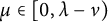 ${\mu \in [0,\lambda -\nu )}$
. This is equivalent to say that
 $(\nu +\mu ,+\infty ) \subset \rho (A)$
, which also implies that
 ${\Sigma ^{+}(A)\subset (-\infty ,\nu +\mu ]}$
and the result follows.
The general structure of
 $\Sigma ^{+}(A)$
is described by the following result.
Proposition 1 [Reference Chu, Liao, Siegmund, Xia and Zhang9, Theorems 2 and 8]
If the evolution operator
 $T(t,s)$
of (2.1) has a forward
 $(K_{0}e^{\mu s},\nu )$
-nonuniform bounded growth, then
 $\Sigma ^{+}(A)$
is the union of m intervals where
 $0<m\leq n$
, such that:
 $$ \begin{align*} \Sigma^{+}(A)=\left\{\begin{array}{@{}c@{}} [a_1,b_1] \\ \text {or}\\ (-\infty,b_1] \end{array}\right\}\cup\;[ a_2,b_2 ]\;\cup\;\cdots\;\cup\;[a_{m-1},b_{m-1}]\;\cup [a_{m},b_{m}]. \end{align*} $$
The intervals
 $[a_{i},b_{i}]$
are called spectral intervals for any
 $i\in \{1,\ldots ,m\}$
. In addition, the intervals
 $\rho _{i+1}(A):=(b_{i},a_{i+1})$
are called spectral gaps. As we assume that (2.1) has a forward nonuniform bounded growth, Lemma 1 ensures the existence of the unbounded spectral gap
 $\rho _{m+1}(A)=(b_{m},+\infty )$
.
The definition of
 $\Sigma ^{+}(A)$
implies that, for any
 $\lambda \in \rho (A)$
, the shifted system (2.3) has a
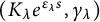 $(K_{\lambda }e^{\varepsilon _{\lambda } s},\gamma _{\lambda })$
-nonuniform exponential dichotomy with projector
 $P_{\lambda }=P_\lambda (\cdot )$
. A thorough examination of [Reference Chu, Liao, Siegmund, Xia and Zhang9, Lemmas 2.4 and 2.7] and [Reference Zhang38, Propositions 2.1–2.4] enables a concise summary of their conclusions regarding projectors and spectral gaps as follows.
Proposition 2 For any
 $\lambda \in \rho (A)$
, the projector
 $P_{\lambda }(\cdot )$
has the following properties:
-
i) The rank of
 $P_{\lambda }(\cdot )$
is constant on any spectral gap.
-
ii) If
$\lambda _{i} \in \rho _{i}(A)$
and
$\lambda _{j} \in \rho _{j}(A)$
with
$i<j$
, then it follows that
$$ \begin{align*}\dim \text{Im}\, P_{\lambda_{i}}<\dim\text{Im}\, P_{\lambda_j}. \end{align*} $$


The above results provide an alternative characterization of the nonuniform contractions stated in Definition 3.
Lemma 2 Assume that (2.1) has a forward
 $(K_{0}e^{\mu s},\nu )$
-nonuniform bounded growth, then it is a
 $(Ke^{\varepsilon s},\gamma )$
-nonuniform exponential contraction if and only if
 $\Sigma ^{+}(A)\subset (-\infty ,0)$
.
Proof Firstly, we assume that
 $\Sigma ^{+}(A)\subset (-\infty ,0)$
. By Proposition 1, we have that
 $(b_{m},+\infty )$
with
 $b_{m}<0$
is a spectral gap. Moreover, statement i) from Proposition 2 implies that the rank of
 $P_{\lambda }(s)$
is constant for any
 $\lambda>b_{m}$
.
When considering
 $\lambda>\nu +\mu $
, Lemma 1 implies that
 $\lambda \in (b_{m},+\infty )$
and also that the shifted system (2.3) has a nonuniform exponential dichotomy with trivial projector
 $P_{\lambda }(s)=I$
. Then, we conclude that
 $P_{\lambda }(s)=I$
for any
 $\lambda>b_{m}$
. Now, as
 $0\in (b_{m},+\infty )$
and the system (2.3) with
 $\lambda =0$
coincides with (2.1), which has a nonuniform exponential dichotomy with projector
 $P(s)=I$
. Then, from Definition 2, it is direct that (2.1) is a
 $(Ke^{\varepsilon s},\gamma )$
-nonuniform exponential contraction.
Secondly, we assume that (2.1) is a
 $(Ke^{\varepsilon s},\gamma )$
-nonuniform exponential contraction, we know that this is equivalent to say that (2.1) has a
 $(Ke^{\varepsilon s},\gamma )$
-nonuniform exponential dichotomy with the identity as projector, whose rank is n. In addition, this also implies that
 $\lambda =0$
is part of some spectral gap.
Note that
 $0\in (b_{m},+\infty )$
. Indeed, otherwise, we would have that
 $0\in (a_{i},b_{i+1})$
with
 $b_{i+1}<a_{m}$
and statement a) from Proposition 2 implies that
 $P_{\lambda }(s)=I$
for any
 ${\lambda \in (a_{i},b_{i+1})}$
. On the other hand, for any
 $\mu>b_{m}$
, we will have that the rank of
 $P_{\mu }$
must be bigger than n, obtaining a contradiction.
Then,
 $0\in (b_{m},+\infty )$
implies that
 $\Sigma ^{+}(A)\subset (-\infty ,b_{m})\subset (-\infty ,0)$
since
 $b_{m}<0$
, and the lemma follows.
2.2 Uniformization lemma
The uniformization lemma offers a method to endow (2.1) with both a uniform exponential dichotomy and uniform bounded growth when it has a nonuniform exponential dichotomy and a forward nonuniform bounded growth. However, the cost is the necessity of operating within a functional framework that is defined by parametrized vector and operator norms. In [Reference Zhou, Lu and Zhang41, p. 697], Zhou, Lu, and Zhang developed this result. As a previous step to its statement, we need to consider a family of norms in
 $\mathbb {R}^{n}$
parametrized by
 $\mathbb {R}_{0}^{+}$
as
 $\left \{|\cdot |_{t}\right \}_{t\in \mathbb {R}_{0}^{+}}$
, that is,
 $|\cdot |_{t}$
is a norm of
 $\mathbb {R}^{n}$
for any
 $t\in \mathbb {R}_{0}^{+}$
. These norms are also known as Lyapunov norms and have been introduced by Barreira and Valls in [Reference Barreira and Valls1, Section 5.4.2] by following an approach inspired in the Lyapunov metric constructed by Pesin [Reference Pesin30, Section 1].
By following [Reference Zhou, Lu and Zhang41], we summarize basic facts about the family
 $\{|\cdot |_{t}\}_{t\in \mathbb {R}_{0}^{+}}$
:
-
a) By the equivalence of norms, there exist two functions
$L_{i}\colon \mathbb {R}_{0}^{+}\to (0,+\infty )$
such that (2.4)
$$ \begin{align} L_{1}(t)|x|\leq |x|_{t} \leq L_{2}(t)|x| \quad \text{for any } t\in \mathbb{R}_0^{+}. \end{align} $$
-
b) The family
$\{|\cdot |_{t}\}_{t\in \mathbb {R}_{0}^{+}}$
is continuous if the mapping
$t\mapsto |x|_{t}$
is continuous on
$\mathbb {R}_{0}^{+}$
for any fixed
$x\in \mathbb {R}^{n}$
. In this case, it follows that the functions
$L_{i}$
from (2.4) are continuous on
$\mathbb {R}_{0}^{+}$
, [Reference Zhou, Lu and Zhang41, Proposition 1]. -
c) A continuous family
$\{|\cdot |_{t}\}_{t\in \mathbb {R}_{0}^{+}}$
is called uniformly lower bounded if
$t\mapsto L_{1}(t)$
is uniformly bounded by a positive constant
$L_{1}>0$
and (2.4) can be replaced by (2.5)
$$ \begin{align} L_{1}|x|\leq |x|_{t} \leq L_{2}(t)|x| \quad \text{for any } t\in \mathbb{R}_0^{+}. \end{align} $$



Remark 1 Given a continuous family of norms
 $\{|\cdot |_{\tau }\}_{\tau \in \mathbb {R}_{0}^{+}}$
defined on
 $\mathbb {R}$
, there exists a continuous function
 $h\colon \mathbb {R}_{0}^{+}\to (0,\infty )$
such that
 $$ \begin{align} |x|_{\tau}=h(\tau)|x| \quad \text{for any } x\in \mathbb{R}. \end{align} $$
In fact, since
 $\{|\cdot |_{\tau }\}_{\tau \in \mathbb {R}_{0}^{+}}$
is a continuous family of norms, we can ensure that for any
 $x\in \mathbb {R}$
:
 $$ \begin{align*}|x|_{\tau}=|x\cdot1|_{\tau}=|x|\cdot|1|_{\tau}=|x|h(\tau),\end{align*} $$
where
 $h(\tau )=|1|_{\tau }$
is a continuous function.
We will assume that
 $\left \{|\cdot |_{t}\right \}_{t\in \mathbb {R}_{0}^{+}}$
is a uniformly lower bounded continuous family of norms. In consequence, we are implicitly assuming that
 $t\mapsto L_{2}(t)$
is an unbounded and continuous function. The following technical result will be useful.
Lemma 3 Given a couple of linear operators
 $U\colon (\mathbb {R}^{n},|\cdot |_{s})\to (\mathbb {R}^{m},|\cdot |_{t})$
and
 $U\colon (\mathbb {R}^{n},|\cdot |)\to (\mathbb {R}^{m},|\cdot |)$
with norms defined by
 $$ \begin{align*}\|U\|_{s,t}= \sup\limits_{x\neq 0}\frac{|Ux|_{t}}{|x|_{s}} \quad \text{and} \quad \|U\|=\sup\limits_{x\neq 0}\frac{|Ux|}{|x|}, \end{align*} $$
it follows that
 $$ \begin{align} \frac{1}{\beta(t)}\|U\|_{s,t}\leq \|U\|\leq \beta(s)\|U\|_{s,t} \quad \text{and} \quad \frac{1}{\beta(s)}\|U\|\leq \|U\|_{s,t}\leq \beta(t)\|U\|, \end{align} $$
where
 $\beta \colon \mathbb {R}_{0}^{+}\to [1,\infty )$
is the continuous and upperly unbounded function:
 $$ \begin{align*} \beta(\tau)=\frac{L_{2}(\tau)}{L_{1}}. \end{align*} $$
Proof By using (2.5), it can be proved that for any
 $x\in \mathbb {R}^{n}$
, it follows that
 $$ \begin{align*}\frac{|Ux|_{t}}{|x|_{s}}\geq \frac{L_{1}}{L_{2}(s)}\frac{|Ux|}{|x|} \quad \text{and} \quad \frac{|Ux|_{t}}{|x|_{s}}\leq \frac{L_{2}(t)}{L_{1}}\frac{|Ux|}{|x|}, \end{align*} $$
and the lemma follows.
Remark 2 Given a linear operator
 $U\colon \mathbb {R}^{p}\to \mathbb {R}^{q}$
and a couple
 $(t,\tau )$
of positive real numbers. It will be useful to recall the estimations
 $$ \begin{align} |U\xi|_{t}\leq \|U\|_{\tau,t}|\xi|_{\tau}, \end{align} $$
 $$ \begin{align} |U\xi|_{\tau}\leq \|U\|_{\tau,\tau}|\xi|_{\tau}, \end{align} $$
 $$ \begin{align} |U\xi|_{\tau}\leq \|U\|_{t,\tau}|\xi|_{t}. \end{align} $$
Lemma 4 (Uniformization Lemma)
The system (2.1) has both a
 $(Ke^{\varepsilon s},\gamma )$
-nonuniform exponential dichotomy and a forward
 $(M(s),\nu )$
-nonuniform bounded growth on
 $\mathbb {R}_0^+$
if and only if there exists a continuous family
 $\left \{|\cdot |_{t}\right \}_{t \in \mathbb {R}_0^+}$
of norms with a uniform lower bound such that (2.1) has a uniform exponential dichotomy with respect to
 $\left \{|\cdot |_{t}\right \}_{t \in \mathbb {R}_{0}^+}$
, i.e., there exist a projection
 $P(t): \mathbb {R}^{n} \rightarrow \mathbb {R}^{n}$
and a couple of constants
 $\alpha>0$
and
 $\kappa \geq 1$
such that the invariant decomposition condition (the last two inequalities in (2.2)) can be replaced by
 $$ \begin{align*}\begin{array}{rr} \left\|T(t, s) P(s)\right\|_{s, t} \leq \kappa e^{-\alpha(t-s)} &\ \mathrm{for}\ t \geq s\geq0 \\ \left\|T(t, s) (I-P(s))\right\|_{s, t} \leq \kappa e^{-\alpha(s-t)} &\ \mathrm{for}\ s \geq t\geq0 \end{array} \end{align*} $$
and a forward
 $(\mu ,\nu )$
-uniform bounded growth with respect to
 $\left \{|\cdot |_{t}\right \}_{t \in \mathbb {R}_{0}^+ }$
, namely,
 $$ \begin{align*}\|T(t, s)\|_{s, t} \leq \mu e^{\nu(t-s)}, \quad t \geq s\geq 0. \end{align*} $$
Remark 3 A meticulous reading of the proof of the Uniformization Lemma [Reference Zhou, Lu and Zhang41, pp. 697–700] shows that the family of norms
 $\{|\cdot |_{t}\}$
verifies
 $|x|_{t}\leq L_{2}(t)|x|$
, where
 $L_{2}(t)= M(t)+K(t)$
.
Remark 4 A version of the Uniformization Lemma, where (2.1) has the properties of
 $(Ke^{\varepsilon _{1} s},\gamma )$
-nonuniform exponential dichotomy and full
 $(Me^{\varepsilon _{2} s},\nu )$
-nonuniform bounded growth, has been used in [Reference Dragičević, Zhang and Zhang15]. Another version has been introduced in [Reference Dragičević13] for nonuniform polynomial dichotomies in evolution equations.
3 Nonuniform conjecture
To set the problem of global nonuniform stability, we have to recall a formal definition of nonuniform asymptotic stability. For this purpose, let us consider the nonlinear system of ordinary differential equations:
 $$ \begin{align} \dot{x} = f(t,x), \end{align} $$
where
 $f\colon \mathbb {R}_{0}^{+}\times \mathbb {R}^{n}\to \mathbb {R}^{n}$
has properties ensuring existence, uniqueness, and unbounded forward continuation of solutions. The solution passing through
 $x_{0}$
at
 $t_{0}$
is denoted by
 $t\mapsto x(t,t_{0},x_{0})$
. We will also assume that
 $f(t,0)=0$
for any
 $t\in \mathbb {R}_{0}^{+}$
.
In addition, it will be useful to recall the comparison functions [Reference Khalil23, Reference Zhou40]:
-
• A function
$\alpha \colon \mathbb {R}_{0}^{+}\to \mathbb {R}_{0}^{+}$
is a
$\mathcal {K}$
function if
$\alpha (0)=0$
and it is nondecreasing. -
• A function
$\alpha \colon \mathbb {R}_{0}^{+}\to \mathbb {R}_{0}^{+}$
is a
$\mathcal {K}_{\infty }$
function if
$\alpha (0)=0$
,
$\alpha (t)\to +\infty $
as
$t\to +\infty $
and it is strictly increasing. -
• A function
$\alpha \colon \mathbb {R}_{0}^{+}\to (0,+\infty )$
is an
$\mathcal {N}$
function if it is nondecreasing. -
• A function
$\alpha (t,s)\colon \mathbb {R}_{0}^{+}\times \mathbb {R}_{0}^{+}\to \mathbb {R}_{0}^{+}$
is a
$\mathcal {KL}$
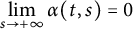
function if
$\alpha (t,\cdot )\in \mathcal {K}$
and
$\alpha (\cdot ,s)$
is decreasing with respect to s and
$\lim \limits _{s\to +\infty }\alpha (t,s)=0$
.







Definition 5 [Reference Karafyllis and Tsinias22, Proposition 2.5] The origin of (3.1) is globally nonuniformly asymptotically stable if for any
 $t_0\geq 0$
and
 $\eta>0$
, there exists
 $\delta :=\delta (t_{0},\eta )>0$
such that
 $$ \begin{align*}|x_{0}|<\delta\Rightarrow|x(t,t_0,x_0)|<\eta,\quad \forall t\geq t_0\geq0 \end{align*} $$
and for any
 $x_{0}\in \mathbb {R}^{n}$
, it follows that
 $\lim \limits _{t\to +\infty }x(t,t_{0},x_{0})=0$
, or equivalently, there exist
 $\sigma \in \mathcal {KL}$
and
 $\theta \in \mathcal {N}$
such that, for any
 $x_{0}\in \mathbb {R}^{n}$
, it follows that
 $$ \begin{align*}|x(t,t_{0},x_{0})|\leq \sigma(\theta(t_{0})|x_{0}|,t-t_{0}). \end{align*} $$
According to [Reference Rugh33], the term nonuniform refers to the fact that the decay of any solution
 $t\mapsto x(t,t_{0},x_{0})$
depends not only on the elapsed time
 $t-t_{0}$
but also on the initial time
 $t_{0}$
. Although this property and its implications have been recognized since the foundational works of Massera [Reference Massera28], examining it through the lenses of dichotomy spectrum and differential Lyapunov inequalities has renewed interest in the topic.
Remark 5 When (3.1) is the linear system (2.1), it can be proved – with the help of
 $\mathcal {KL}$
functions – that if (2.1) has a
 $(Ke^{\varepsilon s},\gamma )$
-nonuniform exponential contraction, then the origin is globally nonuniformly asymptotically stable. In fact, we have
 $$ \begin{align} \sigma(\theta(t_{0})|x_{0}|,t-t_{0})=\theta(t_{0})|x_{0}|e^{-\alpha(t-t_{0})} \,\, \text{and} \,\, \theta(t_{0})=Ke^{\varepsilon t_{0}}. \end{align} $$
Remark 6 Definition 5 is commonly known as global asymptotic stability in the literature. We added the adjective nonuniform motivated by the above remark. This is consistent with the case
 $\theta (t_0)=K$
, which corresponds to the global uniform asymptotic stability.
Statement of the conjecture: As we have set forth the premises now, we are able to state our nonuniform global stability problem.
Conjecture 1 (NU-MYC)
Let us consider the nonlinear system
 $$ \begin{align} \dot{x} = f(t,x), \end{align} $$
where
 $f\colon \mathbb {R}_{0}^{+}\times \mathbb {R}^{n}\to \mathbb {R}^{n}$
. If f satisfies the following conditions:
-
(G1) f is continuous in
$\mathbb {R}_{0}^{+}\times \mathbb {R}^{n}$
and
$C^1$
with respect to x. Moreover, f is such that the forward solutions are defined in
$[t_{0},+\infty )$
for any
$t_{0}\geq 0$
. -
(G2)
$f(t,0)=0$
for all
$t\geq 0$
. -
(G3) For any piecewise continuous function
$t\mapsto \omega (t)$
, the linear system (3.4)where
$$ \begin{align} \dot{\vartheta} = Jf(t,\omega(t))\vartheta, \end{align} $$
$Jf(t,\cdot )$
is the Jacobian matrix of
$f(t,\cdot )$
, has a
$(Ke^{\varepsilon s},\gamma )$
-nonuniform exponential dichotomy spectrum satisfying
$$ \begin{align*} \Sigma^{+} (Jf(t,\omega(t))) \subset (-\infty,0). \end{align*} $$


Then, the origin of (3.3) is globally nonuniformly asymptotically stable.
Condition (G1) establishes rather technical aspects that allow to have a forward solution and condition (G2) emulates the idea of the original conjecture in the non-autonomous framework. On the other hand, condition (G3) deserves several comments:
a) If (G3) is satisfied, Lemma 2 and Remark 5 imply that the systems (3.4) are globally nonuniformly asymptotically stable for any piecewise continuous map. In this context, we recall that a piecewise continuous function is a map
 $\omega \colon \mathbb {R}\to \mathbb {R}^{n}$
having a finite number of first-order discontinuities on any compact interval.
b) The classical Markus–Yamabe conjecture involves the eigenvalue spectrum of the Jacobian matrix associated with the linearized vector field at any given point. In this context, (G3) reflects the aforementioned fact, as both spectra (eigenvalues and nonuniform spectrum) are contained within the interval
 $(-\infty ,0)$
.
c) According to the spectral theory described in Section 2.1 and the fact that a piecewise continuous function is locally integrable, we have well-defined the spectrum
 $\Sigma ^{+} (Jf(t,\omega (t)))$
, for any piecewise continuous function
 $t\mapsto \omega (t)$
.
The following example illustrates a system satisfying assumptions (G1)–(G3).
Example 1 Let us consider the system
 $$ \begin{align} \left\{\begin{array}{@{}ll} \dot{x}_{1} \!\!\!& = a_{1}(t)x_{1}+e^{-t}\tanh(x_{1}+x_{2})\\\dot{x}_{2} \!\!\!& = a_{2}(t)x_{2}+e^{-t}\arctan(x_{2}^{2}), \end{array}\right. \end{align} $$
where
 $$ \begin{align*}a_{1}(t)=6t\sin(t)-2t \quad \text{and} \quad a_{2}(t)=\lambda_{0}+at\sin(t), \end{align*} $$
where
 $\lambda _{0}<a<0$
.
It is easy to see that conditions (G1) and (G2) are fullfilled. In order to verify condition (G3), let us observe that
 $Jf(t,\omega (t))=\operatorname {\mathrm {Diag}}\{a_{1}(t),a_{2}(t)\}+U(t,\omega(t)),$
where
 $U(t,\omega(t))$
is defined by
 $$ \begin{align*} U(t,\omega(t))=\left[\begin{array}{@{}cc@{}} \displaystyle e^{-t}\cosh^{-2}(\omega_{1}(t)+\omega_{2}(t)) & \displaystyle e^{-t}\cosh^{-2}(\omega_{1}(t)+\omega_{2}(t)) \\ 0 & \displaystyle e^{-t}\frac{2\omega_{2}(t)}{1+\omega_{2}(t)^{4}} \end{array}\right]. \end{align*} $$
The scalar equations
 $\dot {x}_{i}=a_{i}(t)x_{i}$
(
 $i=1,2$
) are nonuniformly exponentially stable and we refer the reader to [Reference Vidyasagar37, p. 139] and [Reference Barreira and Valls1, Proposition 2.3] for details, which implies that the diagonal system
 $\dot {x}=\operatorname {\mathrm {Diag}}\{a_{1}(t),a_{2}(t)\}x$
has a nonuniform exponential dichotomy on
 $[0,+\infty )$
with projector
 $P=I$
.
As the off diagonal terms are bounded, the system
 $\dot {x}=Jf(t,\omega (t))x$
can be seen as a bounded perturbation of
 $\dot {x}=\operatorname {\mathrm {Diag}}\{a_{1}(t),a_{2}(t)\}x,$
which vanishes when
 $t\to +\infty $
. Then, by using roughness results (see [Reference Barreira and Valls1, Theorem 3.2] it follows that
 $\dot {x}=Jf(t,\omega (t))x$
has a nonuniform exponential dichotomy on
 $[T,+\infty )$
with projector
 $P(t)=I$
. Finally, we use Lemma 1 from [Reference Castañeda, Huerta and Robledo6] and deduce that the system has a nonuniform exponential dichotomy with projector
 $P=I$
on
 $[0,+\infty ),$
which is equivalent to
 $\Sigma ^{+}(Jf(t,\omega (t)))\subset (-\infty ,0)$
.
A uniform version of the aforementioned conjecture has been recently articulated in [Reference Castañeda and Robledo7], wherein the uniform conjecture was confirmed for scalar systems, triangular systems, and a class of quasilinear systems characterized by appropriate nonlinearity properties.
Remark 7 The NU-MYC is satisfied for dimension
 $n=1$
. In fact, the result follows the lines of [Reference Castañeda and Robledo7, Theorem 1] by using the mean value theorem combined with (G2), which allows to prove that, for any
 $(t_0,x_0)$
fixed, any solution
 $t \mapsto x(t,t_0,x_0)$
of (3.3) can be seen as a solution of the linear system
 $$ \begin{align*}\dot{x}=Jf(t,\omega(t,t_0,x_0))x, \end{align*} $$
where
 $t\mapsto \omega (t,t_0,x_0)$
is piecewise continuous. Then, (G3) together with Lemma 2 and Remark 5 imply that the origin is globally nonuniformly asymptotically stable, where the constants in (3.2) depend on the function
 $t\mapsto \omega (t,t_0,x_0).$
This observation is expected. Several current and historical conjectures regarding global stabilities are easily verified in one-dimensional space. For instance, in addition to the Markus-Yamabe framework, we consider Aizerman’s and Kalman’s conjectures [Reference Vidyasagar37, p. 222]. Despite its apparent triviality, the result of Remark 7 will serve as a useful tool in the subsequent sections.
4 Triangular vector fields
The aim of this section is to prove NU-MYC for triangular vector fields, that is, to show that the origin is globally nonuniformly asymptotically stable for (3.3) when
 $ f(t,x)$
is a triangular vector field.
As previously mentioned in Remark 7, the uniform conjecture has been demonstrated to hold for triangular systems in [Reference Castañeda and Robledo7]. This result can be viewed as a consequence of the scalar case, along with findings by Battelli and Palmer [Reference Battelli and Palmer4] regarding upper triangular systems with diagonal subsystems exhibiting uniform exponential dichotomy. Consequently, to replicate the concepts of the proof for the uniform triangular case, it is essential to extend the Battelli–Palmer result to a nonuniform context.
A first step to cope with this problem is to study the relation between the nonuniform exponential dichotomy properties of the upper block triangular systems
 $$ \begin{align} \dot{z}=\left[\begin{array}{@{}cc@{}} A(t) & C(t)\\ 0 & B(t) \end{array}\right]z, \end{align} $$
with the nonuniform exponential dichotomy properties of the subsystems
 $$ \begin{align} \dot{x}=A(t)x \quad \text{and} \quad \dot{y}=B(t)y, \end{align} $$
where
 $x\in \mathbb {R}^{n}$
,
 $y\in \mathbb {R}^{m}$
,
 $z\in \mathbb {R}^{n+m}$
,
 $A\in M_{n}(\mathbb {R})$
,
 $B\in M_{m}(\mathbb {R}$
), and
 $C\in M_{nm}(\mathbb {R})$
. As we said, this problem has been addressed by Battelli and Palmer [Reference Battelli and Palmer4] in the context of the uniform exponential dichotomy on
 $\mathbb {R}_{0}^{+}$
with an extension to the discrete case in [Reference Battelli, Franca and Palmer3].
In the case of the
 $(K(s),\gamma )$
-nonuniform exponential dichotomy on
 $\mathbb {R}_{0}^{+}$
, a first approach was carried out by Tien, Niehn, and Chien in [Reference Tien, Nhien and Chien36]. In particular, the first result of [Reference Tien, Nhien and Chien36] is as follows.
Proposition 3 (Theorem 2.1 in [Reference Tien, Nhien and Chien36])
If the system (4.1) has a
 $(K(s),\gamma )$
-nonuniform exponential dichotomy on
 $\mathbb {R}_{0}^{+}$
then the decoupled subsystems (4.2) also have a
 $(K(s),\gamma )$
-nonuniform exponential dichotomy on
 $\mathbb {R}_{0}^{+}$
.
As the
 $(Ke^{\varepsilon s},\gamma )$
-nonuniform exponential dichotomy is a particular case of the
 $(K(s),\gamma )$
-nonuniform exponential dichotomy, the following corollary is immediate.
Corollary 1 If the system (4.1) has a
 $(Ke^{\varepsilon s},\gamma )$
-nonuniform exponential dichotomy on
 $\mathbb {R}_{0}^{+}$
then the decoupled subsystems (4.2) also have a
 $(Ke^{\varepsilon s},\gamma )$
-nonuniform exponential dichotomy on
 $\mathbb {R}_{0}^{+}$
.
Our next result will show the converse of Proposition 3, which follows the lines of the result proved by Battelli and Palmer in [Reference Battelli and Palmer4, Theorem 1] but imposes boundedness conditions for C in terms of matrix norms
 $\|\cdot \|_{t,t}$
described in Section 2.2 and also incorporates a creative use of the Uniformization Lemma.
Let us recall we are assuming that (2.1) has the property of forward
 $(Me^{\delta s},\nu )$
-nonuniform bounded growth and a
 $(Ke^{\varepsilon s},\gamma )$
-nonuniform exponential dichotomy on
 $\mathbb {R}_{0}^{+}$
. Then, by using the Uniformization Lemma and Remark 3, we have that the continuous norms
 $\{|\cdot |_{t}\}$
satisfy the inequalities
 $$ \begin{align} L_{1}|x|\leq |x|_{t} \leq \underbrace{(M+K)}_{:=L_{2}}e^{\theta t}|x| \quad \text{for any } t\in \mathbb{R}_0^{+}, \end{align} $$
for some
 $L_{1}>0$
, where
 $\theta :=\max \{\delta ,\varepsilon \}$
. By considering these specific norms, the inequalities (2.7) become
 $$ \begin{align} \frac{1}{L}e^{-\theta t}\|U\|_{s,t}\leq \|U\|\leq Le^{\theta s}\|U\|_{s,t} \,\, \text{and} \,\,\, \frac{1}{L}e^{-\theta s}\|U\|\leq \|U\|_{s,t}\leq Le^{\theta t}\|U\|, \end{align} $$
where
 $L=L_{2}/L_{1}$
. Now, the converse result of Corollary 1 is given by the following.
Theorem 1 Let us consider the upper block triangular system (4.1). If
-
i) the decoupled systems (4.2) have the property of forward
$(M e^{\ell s},\omega )$
-nonuniform bounded growth and forward
$(\tilde {M} e^{\tilde {\ell } s},\tilde {\omega })$
-nonuniform bounded growth, respectively, on
$\mathbb {R}_{0}^{+}$
; -
ii) the decoupled systems (4.2) have the properties of
$(K e^{\varepsilon s},\alpha )$
-nonuniform exponential dichotomy and
$(\tilde {K} e^{\tilde {\varepsilon } s},\tilde {\alpha })$
-nonuniform exponential dichotomy, respectively, on
$\mathbb {R}_{0}^{+}$
; -
iii) the nondiagonal block verifies
(4.5)where
$$ \begin{align} \|C\|_{\tau,\infty}:=\sup\limits_{\tau\in \mathbb{R}_{0}^{+}}\|C(\tau)\|_{\tau,\tau}< \infty, \end{align} $$
$$ \begin{align*}\|C(\tau)\|_{\tau,\tau}= \sup\limits_{x\neq 0}\frac{|C(\tau)x|_{\tau}}{|x|_{\tau}} \quad \mathrm{with}\ |\cdot|_{\tau}\ \mathrm{verifying}\ (4.3), \end{align*} $$


then (4.1) also has a
 $(\bar {K}e^{\bar {\varepsilon } s},\bar {\alpha })$
-nonuniform exponential dichotomy on
 $\mathbb {R}_{0}^{+}$
, where
 $\bar {K}$
is a constant dependent of
 $\alpha $
and
 $\tilde {\alpha }$
,
 $\bar {\varepsilon }\geq 0$
and
 $\bar {\alpha }=\min \{\alpha , \widetilde {\alpha }\}$
, and a forward
 $(\bar {M} e^{\bar {\theta } s},\bar {\omega })$
-nonuniform bounded growth on
 $\mathbb {R}_{0}^{+}$
.
The proof of this result is plenty of bulky technicalities and the Uniformization Lemma combined with the functional setting from [Reference Zhou, Lu and Zhang41] play a key role. In order to give continuity to the reading of the article, the proof is written in the Appendix.
Remark 8 A result related to Theorem 1 was formulated in terms of tempered exponential dichotomies by Barreira and Valls in [Reference Barreira and Valls2, Theorem 2.3], which does not include the
 $(Ke^{\varepsilon s},\gamma )$
-nonuniform exponential dichotomy considered in Theorem 1. In fact, our nonuniform term
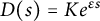 $D(s)=Ke^{\varepsilon s}$
with
 $\varepsilon>0$
verifies the asymptotic behavior
 $$ \begin{align*}\limsup\limits_{s\to \infty}\frac{D(s)}{s}=\infty>0, \end{align*} $$
which is just the opposite to the property considered in [Reference Barreira and Valls2].
Remark 9 By using the left inequality (4.4), we have that
 $\|C(\tau )\|_{\tau ,\tau }\leq Le^{\theta \tau }\|C(\tau )\|$
for any
 $\tau \geq 0$
. In consequence, a sufficient condition ensuring (4.5) is given by
 $$ \begin{align} \sup\limits_{\tau\in\mathbb{R}_{0}^{+}}Le^{\theta \tau}\|C(\tau)\|<\infty, \end{align} $$
this means, for example, that if
 $C(\tau )=e^{-\psi \tau }C_{0}(\tau )$
, where
 $\psi \geq \theta $
and
 $C_{0}$
is bounded on
 $\mathbb {R}_{0}^{+}$
, then the last inequality is satisfied.
The following scalar example indicates that the condition (4.6) is sufficient but not necessary in order to the expression (4.5) will be satisfied.
Example 2 Given
 $\tau \in \mathbb {R}_{0}^{+}$
, let us consider
 $c(\tau ):(\mathbb {R},|\cdot |_{\tau })\rightarrow (\mathbb {R},|\cdot |_{\tau })$
such that
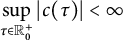 $\displaystyle \sup _{\tau \in \mathbb {R}_{0}^{+}}|c(\tau )|<\infty $
, then by considering Remark 1, we have that
 $$ \begin{align*} \begin{array}{@{}rcl@{}} \|c(\tau)\|_{\tau,\tau}&=&\displaystyle\sup_{x\neq0}\frac{|c(\tau)x|_{\tau}}{|x|_{\tau}}=\displaystyle\sup_{x\neq0}\frac{h(\tau)|c(\tau)x|}{h(\tau)|x|}=|c(\tau)| \end{array} \end{align*} $$
and we conclude that
 $\displaystyle \sup _{\tau \in \mathbb {R}_{0}^{+}}\|c(\tau )\|_{\tau ,\tau }=\displaystyle \sup _{\tau \in \mathbb {R}_{0}^{+}}|c(\tau )|<\infty $
.
Corollary 2 If the upper block system
 $$ \begin{align} \dot{x}=\left[\begin{array}{@{}cccc@{}} A_{1}(t) & C_{12}(t) & \cdots & C_{1k}(t)\\ 0 & A_{2}(t) &\cdots & C_{2k}(t)\\ \vdots & & \ddots & \\ 0 & \cdots & \cdots & A_{k}(t) \end{array}\right] x \quad \end{align} $$
is such that the diagonal subsystems
 $$ \begin{align*} \dot{x}_{i}=A_{i}(t)x_{i} \quad \mathrm{for}\ i=1,\ldots,k \end{align*} $$
have the properties of
 $(K_{i}e^{\varepsilon _{i}s},\alpha _{i})$
-nonuniform exponential dichotomy and
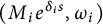 $(M_{i}e^{\delta _{i} s},\omega _{i})$
-nonuniform bounded growth on
 $\mathbb {R}_{0}^{+}$
and the upper diagonal blocks verify
 $$ \begin{align} \sup\limits_{\tau\in \mathbb{R}_{0}^{+}}\|C_{j}(\tau)\|_{\tau,\tau}<\infty\; \mathrm{for\ any}\ j\in \{2,\ldots,k\}, \; \mathrm{where}\ C_{j}(t)=\left[\begin{array}{@{}c@{}} C_{1j}(t)\\ C_{2j}(t)\\ \vdots \\ C_{j-1\,j}(t) \end{array}\right], \end{align} $$
then (4.7) has the properties of
 $(Ke^{\varepsilon s},\alpha )$
-nonuniform exponential dichotomy on
 $\mathbb {R}_{0}^{+}$
and forward
 $(Me^{\delta s},\omega )$
-nonuniform bounded growth on
 $\mathbb {R}_{0}^{+}$
.
Proof The proof will be carried out recursively.
If
 $k=2$
, the result is an immediate consequence of Theorem 1 since the matrix of the system (4.7) has similar structure to (4.1) with
 $A_{1}(t)=A(t)$
,
 $A_{2}(t)=B(t),$
and
 $C_{12}(t)=C(t)$
.
If
 $k=3$
, the system (4.7) can be seen as having a similar structure that (4.1) with
 $$ \begin{align*} A(t)=\left[\begin{array}{@{}cc@{}} A_{1}(t) & C_{12}(t)\\ 0 & A_{2}(t) \end{array}\right], \quad B(t)=A_{3}(t) \quad \text{and} \quad C(t)=C_{3}(t)=\left[\begin{array}{@{}c@{}} C_{13}(t)\\ C_{23}(t) \end{array}\right]. \end{align*} $$
Note that the subsystems
 $\dot {x}=A(t)x$
and
 $\dot {y}=B(t)y$
have a nonuniform exponential dichotomy on
 $\mathbb {R}_{0}^{+}$
. The first dichotomy property is a consequence of the case
 $k=2$
while the second one is a hypothesis. As (4.8) is fulfilled for
 $j=3$
, Theorem 1 implies that the system (4.7) with
 $k=3$
has a nonuniform exponential dichotomy on
 $\mathbb {R}_{0}^{+}$
and the proof is achieved by a recursive way for
 $k\geq 4$
.
A particular – but important – byproduct of the above corollary is the following result when all the diagonal terms
 $A_{i}(t)$
are scalar functions.
Corollary 3 If the upper triangular system
 $$ \begin{align} \dot{x}=\left[\begin{array}{@{}cccc@{}} a_{1}(t) & c_{12}(t) & \cdots & c_{1n}(t)\\ 0 & a_{2}(t) &\cdots & c_{2n}(t)\\ \vdots & & \ddots & \\ 0 & \cdots & \cdots & a_{n}(t) \end{array}\right] x \quad \end{align} $$
is such that all the scalar differential equations
 $$ \begin{align} \dot{x}_{i}=a_{i}(t)x_{i} \quad \mathrm{for\ any}\ i=1,\ldots,n \end{align} $$
have the properties of forward (
 $M_ie^{\theta _{i}s},\omega _{i}$
)-nonuniform bounded growth property on
 $\mathbb {R}_{0}^{+}$
and
 $(K_{i}e^{\varepsilon _{i}s},\alpha _{i})$
-nonuniform exponential dichotomy on
 $\mathbb {R}_{0}^{+}$
and the upper triangular terms verify
 $$ \begin{align} \sup\limits_{\tau\in\mathbb{R}_{0}^{+}}\|C_{j}(\tau)\|_{\tau,\tau}=\sup\limits_{\tau\in\mathbb{R}_{0}^{+}}\left|\left|\left(\begin{array}{@{}c@{}} c_{1j}(\tau)\\ c_{2j}(\tau)\\ \vdots \\ c_{j-1\,j}(\tau) \end{array}\right)\right|\right|_{\tau,\tau}<\infty \quad \mathrm{for\ any}\ j\in \{2,\ldots,n\}, \end{align} $$
then (4.9) has the properties of
 $(Ke^{\varepsilon s},\alpha )$
-nonuniform exponential dichotomy on
 $\mathbb {R}_{0}^{+}$
and forward
 $(Me^{\delta s},\omega )$
-nonuniform bounded growth on
 $\mathbb {R}_{0}^{+}$
.
Remark 10 Note that, when
 $j=2$
in (4.11), we have
 $$ \begin{align*}\sup\limits_{\tau\in\mathbb{R}_{0}^{+}}\|C_{2}(\tau)\|_{\tau,\tau}=\sup\limits_{\tau\in\mathbb{R}_{0}^{+}}\|c_{12}(\tau)\|_{\tau,\tau}=\sup\limits_{\tau\in\mathbb{R}_{0}^{+}}\sup\limits_{x\neq0}\frac{|c_{12}(\tau)x|_{\tau}}{|x|_{\tau}}<\infty, \end{align*} $$
and in this case, the family of norms
 $\{|\cdot |_{\tau }\}_{\tau \in \mathbb {R}_{0}^{+}}$
satisfies (2.6).
Remark 11 When we consider that
 $n=2$
in (4.9), the scalar equations (4.10) admit a
 $(K_ie^{\varepsilon _{i}s},\alpha _{i})$
-nonuniform exponential dichotomy on
 $\mathbb {R}_{0}^{+}$
and a forward
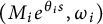 $(M_ie^{\theta _{i}s},\omega _{i})$
-nonuniform bounded growth property on
 $\mathbb {R}_{0}^{+}$
, with
 $i=1, 2$
and as in Example 1, we assume that
 $$ \begin{align*}\sup\limits_{\tau\in\mathbb{R}_{0}^{+}}|c_{12}(\tau)|<\infty,\end{align*} $$
then Corollary 3 allow us to ensure that the system
 $$ \begin{align*} \dot{x}=\left[\begin{array}{@{}cc@{}} a_{1}(t) & c_{12}(t)\\ 0 & a_{2}(t) \end{array}\right] x \end{align*} $$
has a
 $(Ke^{\varepsilon s},\alpha )$
-nonuniform exponential dichotomy on
 $\mathbb {R}_{0}^{+}$
.
Remark 12 In [Reference Palmer29, Theorem 1], a related result to Corollary 3 is proved in a context of uniform exponential dichotomy on the half line. The proof is made without using parametrized norms.
Lemma 5 Under the assumptions of Corollary 1 and Theorem 1, the
 $(Ke^{\varepsilon s},\alpha )$
-nonuniform exponential dichotomy spectrum of the upper block system (4.1) verifies
 $$ \begin{align*} \Sigma^{+}(A)\cup \Sigma^{+}(B) =\Sigma^{+}(U) \quad \mathrm{with} \quad U=\left(\begin{array}{@{}cc@{}} A& C \\ 0 & B \end{array}\right). \end{align*} $$
Proof As the hypothesis of Theorem 1 is verified, it follows that the diagonal subsystems
 $\dot {x}=A(t)x$
and
 $\dot {y}=B(t)y$
have, respectively, the properties of forward
 $(M e^{\ell s},\omega )$
-nonuniform bounded growth and forward
 $(\tilde {M} e^{\tilde {\ell } s},\tilde {\omega })$
-nonuniform bounded growth on
 $\mathbb {R}_{0}^{+}$
. Now, Lemma 1 implies that
 $$ \begin{align*}\Sigma^{+}(A)\subset (-\infty,\ell+\omega] \quad \text{and} \quad \Sigma^{+}(B)\subset (-\infty,\tilde{\ell}+\tilde{\omega}], \end{align*} $$
which imply that
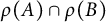 $ \rho (A)\cap \rho (B)$
is not empty. Indeed, otherwise, we will have that
 $\mathbb {R}=[\rho (A)\cap \rho (B)]^{c}=\Sigma ^{+}(A)\cup \Sigma ^{+}(B)$
and then, at least one the spectra
 $\Sigma ^{+}(A)$
or
 $\Sigma ^{+}(B)$
must be upperly unbounded, obtaining a contradiction.
For any
 $\lambda \in \rho (A)\cap \rho (B)$
, we have that the subsystems
 $$ \begin{align} \dot{x}=[A(t)-\lambda I]x \quad \text{and} \quad \dot{y}=[B(t)-\lambda I]y \end{align} $$
have a nonuniform exponential dichotomy on
 $\mathbb {R}_{0}^{+}$
. In addition, it is straightforward to verify that we also have the property of forward nonuniform bounded growth on
 $\mathbb {R}_{0}^{+}$
. In consequence, Theorem 1 applied to the shifted system
 $\dot {z}=[U(t)-\lambda I]z$
implies that
 $\lambda \in \rho (U)$
and it follows that
 $\rho (A)\cap \rho (B)\subset \rho (U)$
.
Finally, if
 $\lambda \in \rho (U)$
, Corollary 1 implies that the subsystems (4.12) have a nonuniform exponential dichotomy on
 $\mathbb {R}_{0}^{+}$
, which is equivalent to
 $\lambda \in \rho (A)\cap \rho (B)$
, which implies that
 $\rho (U)\subset \rho (A)\cap \rho (B)$
and the result follows.
Based on a recursive application of Lemma 5, we obtain the following descriptions for the nonuniform exponential dichotomy spectrum for an upper block system as in (4.7) and for an upper triangular system as in (4.9), respectively.
Corollary 4 Under the assumptions of Corollary 2, the nonuniform exponential dichotomy spectrum of the upper block system (4.7) is described by
 $$ \begin{align*}\Sigma^{+}(A_{1})\cup \Sigma^{+}(A_{2})\cup \cdots \cup\Sigma^{+}(A_{k}). \end{align*} $$
Corollary 5 Under the assumptions of Corollary 3, the nonuniform exponential dichotomy spectrum of the upper triangular system (4.9) is described by
 $$ \begin{align*}\Sigma^{+}(a_{1})\cup \Sigma^{+}(a_{2})\cup \cdots \cup\Sigma^{+}(a_{n}). \end{align*} $$
Remark 13 The aforementioned states that the nonuniform exponential dichotomy spectrum of an upper triangular system corresponds to the union of the spectra of the scalar equations (4.10). The concept referred to as diagonal significance was introduced for the discrete uniform exponential dichotomy spectrum by Pötzsche in [Reference Pötzsche31]. This fact is evident in the autonomous case; however, it is not consistently verified in the nonautonomous framework, which may seem counterintuitive.
Theorem 1 and its consequences provide the framework to state and prove our main result, namely, the nonautonomous NU-MYC is satisfied for triangular system of nonautonomous differential equations whose nondiagonal parts satisfy boundedness conditions described in terms of parametrized norms.
Theorem 2 Let us consider the triangular system
 $$ \begin{align} \begin{array}{@{}rcr@{}} \dot{x}_{1}&=&f_{1}(t,x_{1},x_{2},\ldots,x_{n})\\ \dot{x}_{2}&=&f_{2}(t,x_{2},\ldots,x_{n})\\ &\vdots& \\ \dot{x}_{n}&=&f_{n}(t,x_{n}), \end{array} \end{align} $$
whose right part, namely,
 $F(t,x)$
, verifies (G1) and (G2). If for any piecewise continuous function
 $t\mapsto \theta (t),$
it is fulfilled that
-
(a) There exist constants
$k_{i}\geq 1$
,
$\alpha _{i}>0,$
and
$\varepsilon _{i}\in [0,\alpha _{i})$
such that
$$ \begin{align*}\kern-5pt \int_{s}^{t}\frac{\partial f_{i}}{\partial x_{i}}(\tau,\theta(\tau))\,d\tau \leq \ln(k_{i})-\alpha_{i}(t-s)+\varepsilon_{i}s \quad \text{for any } t\geq s\geq 0 \text{ and } i=1,\ldots,n. \end{align*} $$
-
(b) For any
$j\in \{2,\ldots ,n\}$
and any piecewise continuous function
$t\mapsto \theta (t)$
, the partial derivatives verify
$$ \begin{align*} \displaystyle \sup\limits_{\tau\in\mathbb{R}_{0}^{+}}\left\|\mathcal{F}_{j}(\tau)\right\|_{\tau,\tau}=\sup\limits_{\tau\in\mathbb{R}_{0}^{+}}\sup\limits_{x\neq0}\displaystyle\frac{|\mathcal{F}_{j}(\tau)x|_{\tau}}{|x|_{\tau}}<\infty,\ \mathrm{with}\ \mathcal{F}_{j}(\tau)=\begin{pmatrix} \frac{\partial f_{1}(\tau,\theta(\tau))}{\partial x_{j}}\\\\ \frac{\partial f_{2}(\tau,\theta(\tau))}{\partial x_{j}}\\ \vdots \\ \frac{\partial f_{j-1}(\tau,\theta(\tau))}{\partial x_{j}} \end{pmatrix}, \end{align*} $$





then the trivial solution of (4.13) is globally nonuniformly asymptotically stable.
Proof Firstly, we will prove that (G3) is satisfied. In fact, statement (a) implies that, for any
 $i=1,\ldots ,n$
, the nonuniform exponential dichotomy spectra of the differential equations
 $$ \begin{align*}\dot{x}=\frac{\partial f_i}{\partial x_i}(t,\theta(t))x \end{align*} $$
verify
 $$ \begin{align} \Sigma^{+}\left[\frac{\partial f_i}{\partial x_i}(t,\theta(t))\right] \subset (-\infty, 0) \end{align} $$
for any piecewise continuous function
 $t\mapsto \theta (t)=(\theta _{1}(t),\ldots ,\theta _{n}(t))$
.
On the other hand, let us recall that the Jacobian matrix
 $JF$
is upper triangular defined by
 $$ \begin{align*} JF(t,x_{1},\ldots,x_{n})_{ij}=\left\{ \begin{array}{@{}ccl@{}} \frac{\partial f_{i}}{\partial x_{j}}(t,x_{i},\ldots,x_{n}) &\text{if}& i\leq j, \\ 0 &\text{if} & i>j. \end{array}\right. \end{align*} $$
Then, statement (b), combined with (4.14) and Corollary 5, implies that
 $$ \begin{align*} \Sigma^{+}\left [JF(t,\theta(t)) \right ]= \bigcup\limits_{i=1}^{n} \Sigma^{+}\left[\frac{\partial f_i}{\partial x_i}(t,\theta(t))\right]\subset (-\infty,0) \end{align*} $$
and (G3) follows.
Let
 $t\mapsto (x_1(t),x_2(t),\ldots ,x_n(t))$
be a solution of (4.13) passing through
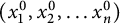 $(x_{1}^0,x_{2}^0, \ldots x_{n}^0)$
at
 $t=t_{0}$
. Note that the scalar equation
 $$ \begin{align*}\dot{x}_{n}=f_{n}(t,x_{n}) \quad \text{with} \quad x_{n}(t_{0})=x_{n}^{0} \end{align*} $$
is a subsystem of (4.13) whose solution is denoted by
 $\phi _{n}(t):=x_{n}(t,t_{0},x_{n}^{0})$
and verifies
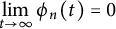 $\lim \limits _{t\to \infty }\phi _{n}(t)=0$
globally and nonuniformly, as we can see by Remark 7.
Now, we can see that the last two equations of (4.13) are
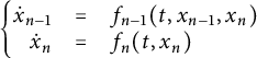 $$ \begin{align*} \left\{\begin{array}{@{}rcl@{}} \dot{x}_{n-1}&=&f_{n-1}(t,x_{n-1},x_{n})\\ \dot{x}_{n}&=&f_{n}(t,x_{n}) \end{array}\right. \end{align*} $$
with initial conditions
 $(x_{n-1}^{0},x_{n}^{0})$
at
 $t=t_{0}$
. The solution of this system is denoted by
 $(\phi _{n-1}(t),\phi _{n}(t))$
, where
 $\phi _{n}$
is defined above and
 $\phi _{n-1}$
is the solution of the scalar equation
 $$ \begin{align*}\dot{x}_{n-1}=f_{n}(t,x_{n-1},\phi_{n}(t)) \quad \text{with} \quad x_{n-1}(t_{0})=x_{n-1}^{0} \end{align*} $$
and, as before, also verifies
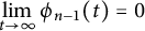 $\lim \limits _{t\to \infty }\phi _{n-1}(t)=0$
globally and nonuniformly, as we can see again by Remark 7. The rest of the proof can be achieved in a recursive way.
Remark 14 We point out that the system (3.5) described in Example 1 fulfills the assumptions of Theorem 2. In fact, as we have seen in Example 1, we know that
 $\Sigma ^{+}\left (\frac {\partial f_{i}}{x_{i}}(t,\theta (t))\right )\subset (-\infty ,0)$
with
 $i=1,2$
. By using Lemma 2, we also know this property is equivalent to assumption (a).
In order to verify statement (b) from Theorem 2, notice that
 $$ \begin{align*} \sup\limits_{\tau\in\mathbb{R}_{0}^{+}}\left\|\mathcal{F}_{j}(\tau)\right\|_{\tau,\tau}=\sup\limits_{\tau\in\mathbb{R}_{0}^{+}}\left\|\frac{\partial f_{1}}{\partial x_{2}}(\tau,\theta (\tau))\right\|_{\tau,\tau}=\sup\limits_{\tau \in \mathbb{R}_{0}^{+}} e^{-t}\cosh^{-2}(\theta_{1}(t)+\theta_{2}(t)) <\infty, \end{align*} $$
where the last identity is a consequence of Example 2.
5 An example arising from control theory
Let us consider the nonlinear control system:
 $$ \begin{align} \left(\begin{array}{@{}c@{}} \dot{x}_{1} \\ \dot{x}_{2} \end{array}\right)&=\left[\begin{array}{@{}cc@{}} 1 & 0 \\ 0 & b(t) \end{array} \right]\left(\begin{array}{@{}c@{}} x_{1} \\ x_{2} \end{array}\right)+u(t)x_{1}\end{align} $$
 $$ \begin{align} y=\left(\begin{array}{@{}c@{}} x_{1}^{2}+x_{2}^{2} \\ x_{2} \end{array}\right), \end{align} $$
under the assumption that
 $\Sigma ^{+}(b)\subset (-\infty ,0)$
, or equivalently, the scalar equation
 ${\dot {x}_{2}=b(t)x_{2}}$
is a nonuniform exponential contraction.
In the language of control theory, the map
 $y\colon \mathbb {R}^{2}\to \mathbb {R}^{2}$
described by (5.2) is known as the output of the control system and denotes what can be effectively measured of the system. On the other hand, the map
 $u\colon \mathbb {R}^{2}\to \mathbb {R}$
is known as the input of the control system. In this context, the uncontrolled part of the system, namely, the linear system
 $$ \begin{align*} \left(\begin{array}{@{}c@{}} \dot{x}_{1} \\ \dot{x}_{2} \end{array}\right)=\left[\begin{array}{@{}cc@{}} 1 & 0 \\ 0 & b(t) \end{array} \right]\left(\begin{array}{@{}c@{}} x_{1} \\ x_{2} \end{array}\right) \end{align*} $$
is usually named as the plant of the system. We refer to [Reference Rugh33, Reference Sontag35, Reference Vidyasagar37] for additional details about control systems.
As the plant is unstable, the goal is to construct a feedback control law, namely, an input
 $u(\cdot )$
defined in terms of the nonlinear output
 $y(x_{1},x_{2})$
, in order to stabilize the system. In this context, we propose the following control law:
 $$ \begin{align} u(y)=u(x_{1}^{2}+x_{2}^{2},x_{2})=a(t)-1+\frac{e^{-t}x_{2}}{x_{1}^{2}+x_{2}^{2}+1}, \end{align} $$
where
 $\Sigma ^{+}(a)\subset (-\infty ,0)$
.
Upon inserting (5.3) into (5.1), we obtain the nonlinear system
 $$ \begin{align*} \left\{\begin{array}{@{}rcl@{}} \dot{x}_{1} &=& \displaystyle a(t)x_{1}+\frac{e^{-t}x_{1}x_{2}}{x_{1}^{2}+x_{2}^{2}+1}\\ \dot{x}_{2} &=& \displaystyle b(t)x_{2}. \end{array}\right. \end{align*} $$
It is direct to see that assumptions (G1) and (G2) are fulfilled. Now, we will verify that the assumptions of Theorem 2 are also satisfied. In fact, statement (a) for
 $i=2$
follows directly from
 $\Sigma ^{+}(b)\subset (-\infty ,0)$
. In order to study the case
 $i=1,$
notice that
 $$ \begin{align*} \frac{\partial f_{1}}{\partial x_{1}}(x_{1},x_{2}) = a(t)+e^{-t}\frac{(1-x_{1}^{2}+x_{2}^{2})x_{2}}{(x_{1}^{2}+x_{2}^{2}+1)^{2}}. \end{align*} $$
As the second term is bounded, the scalar equation
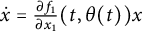 $\dot {x}=\frac {\partial f_{1}}{\partial x_{1}}(t,\theta (t))x$
can be seen as a bounded perturbation of
 $\dot {x}=a(t)x,$
which vanishes when
 $t\to +\infty $
. Then, by using roughness results (see [Reference Barreira and Valls1, Theorem 3.2]), combined with
 $\Sigma ^{+}(a)\subset (-\infty ,0),$
it follows that
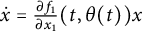 $\dot {x}=\frac {\partial f_{1}}{\partial x_{1}}(t,\theta (t))x$
has a nonuniform exponential dichotomy on
 $[T,+\infty )$
with projector
 $P(t)=1$
. Finally, we use Lemma 1 from [Reference Castañeda, Huerta and Robledo6] and deduce that the system has a nonuniform exponential dichotomy with projector
 $P=1$
on
 $[0,+\infty ),$
which is equivalent to
 $\Sigma ^{+}\left (\frac {\partial f_{1}}{\partial x_{1}}(t,\theta (t))\right )\subset (-\infty ,0)$
.
In order to verify statement (b) from Theorem 2, notice that
 $$ \begin{align*} \sup\limits_{\tau\in\mathbb{R}_{0}^{+}}\left\|\mathcal{F}_{j}(\tau)\right\|_{\tau,\tau}=\sup\limits_{\tau\in\mathbb{R}_{0}^{+}}\left\|\frac{\partial f_{1}}{\partial x_{2}}(\tau,\theta (\tau))\right\|_{\tau,\tau}=\sup\limits_{\tau \in \mathbb{R}_{0}^{+}}e^{-\tau}\frac{(1-\theta_{1}^{2}+\theta_{2}^{2})\theta_{2}}{(\theta_{1}^{2}+\theta_{2}^{2}+1)^{2}}<\infty, \end{align*} $$
where the last identity is a consequence of Example 2. Therefore, by using Theorem 2, we can see that the feedback control law (5.3) stabilizes the nonlinear control system (5.1) in a nonuniform exponential way.
Appendix A Proof of Theorem 1
A.1 Preliminaries
By hypothesis, we know that the linear systems
 $\dot {x}=A(t)x$
and
 $\dot {y}=B(t)y$
have a
 $(Ke^{\varepsilon s},\alpha )$
and
 $(\tilde {K}e^{\tilde {\varepsilon }s},\tilde {\alpha })$
-nonuniform exponential dichotomy on
 $\mathbb {R}_{0}^{+}$
with projectors
 $P^{A}(\cdot )$
and
 $P^{B}(\cdot ),$
respectively:
 $$ \begin{align} \begin{array}{@{}rcl@{}} \|X(t,s)P^{A}(s)\| &\leq & Ke^{-\alpha(t-s)+\varepsilon s} \quad \text{for } t\geq s\geq 0,\\ \|X(t,s)[I_{n}-P^{A}(s)]\|&\leq & Ke^{-\alpha(s-t)+\varepsilon s} \quad \text{for } s\geq t\geq 0, \end{array} \end{align} $$
and
 $$ \begin{align} \begin{array}{@{}rcl@{}} \|Y(t,s)P^{B}(s)\| &\leq & \tilde{K}e^{-\widetilde{\alpha}(t-s)+\tilde{\varepsilon}s} \quad \text{for } t\geq s\geq 0,\\ \|Y(t,s)[I_{m}-P^{B}(s)]\|&\leq & \tilde{K}e^{-\widetilde{\alpha}(s-t)+\tilde{\varepsilon}s} \quad \text{for } s\geq t\geq 0, \end{array} \end{align} $$
where
 $X(t,s)$
and
 $Y(t,s)$
are its corresponding evolution operators. We also know that the above subsystems have the properties of forward
 $(Me^{ \ell s},\omega )$
and
 $(\tilde {M}e^{\tilde {\ell } s},\tilde {\omega })$
-nonuniform bounded growth on
 $\mathbb {R}_{0}^{+}$
, respectively, that is,
 $$ \begin{align} \|X(t,s)\| \leq Me^{\omega(t-s)+\ell s} \quad \text{and} \quad \|Y(t,s)\|\leq \tilde{M}e^{\tilde{\omega}(t-s)+\tilde{\ell} s} \quad \text{for } t\geq s\geq 0, \end{align} $$
then, the Uniformization Lemma can be applied to both subsystems. On the one hand, the dichotomy estimations become
 $$ \begin{align*}\begin{array}{@{}rr@{}} \left\|X(t, s) P^{A}(s)\right\|_{s, t} \leq \kappa e^{-\alpha(t-s)} & \text{ for } t \geq s\geq0, \\ \left\|X(t, s) [I_{n}-P^{A}(s)]\right\|_{s, t} \leq \kappa e^{-\alpha(s-t)} & \text{ for } s \geq t\geq0, \end{array} \end{align*} $$
and
 $$ \begin{align*}\begin{array}{@{}rr@{}} \left\|Y(t, s) P^{B}(s)\right\|_{s, t} \leq \tilde{\kappa} e^{-\tilde{\alpha}(t-s)} & \text{ for } t \geq s\geq0, \\ \left\|Y(t, s) [I_{m}-P^{B}(s)]\right\|_{s, t} \leq \tilde{\kappa} e^{-\tilde{\alpha}(s-t)} & \text{ for } s \geq t\geq 0, \end{array} \end{align*} $$
while the forward bounded growth properties become
 $$ \begin{align} \|X(t, s)\|_{s, t} \leq \mu e^{\omega(t-s)} \quad \text{and} \quad \|Y(t, s)\|_{s, t} \leq \tilde{\mu} e^{\tilde{\omega}(t-s)}\quad t \geq s\geq 0. \end{align} $$
The Uniformization Lemma also ensures the existence of two families of norms: a family
 $\{|\cdot |_{t}^{A}\}_{t}$
in
 $\mathbb {R}^{n}$
another one
 $\{|\cdot |_{t}^{B}\}_{t}$
in
 $\mathbb {R}^{m}$
. The inequalities (2.5) are verified with
 $L_{1}^{A}$
,
 $L_{1}^{B}$
,
 $L_{1}^{A}(t),$
and
 $L_{2}^{B}(t),$
respectively. By Remark 3, we know that
 $$ \begin{align*} L_{2}^{A}(t)=Me^{\ell t}+Ke^{\varepsilon t} \quad \text{and} \quad L_{2}^{B}(t)=\tilde{M}e^{\tilde{\ell} t}+\tilde{K}e^{\tilde{\varepsilon} t} \end{align*} $$
and the inequalities (2.7) are verified with
 $$ \begin{align} \beta^{A}(t)=\frac{L_{2}^{A}(t)}{L_{1}^{A}}\leq Le^{\theta t} \quad \text{and} \quad \beta^{B}(t)=\frac{L_{2}^{B}(t)}{L_{1}^{B}}\leq Le^{\theta t}, \end{align} $$
where
 $$ \begin{align} L=\max\left\{\frac{M+K}{L_{1}^{A}},\frac{\tilde{M}+\tilde{K}}{L_{1}^{B}}\right\} \quad \text{and} \quad \theta=\max\{\ell,\tilde{\ell},\varepsilon,\tilde{\varepsilon}\}. \end{align} $$
These constants L and
 $\theta $
are useful to state the following result.
Lemma A.1 For any
 $t,\tau ,s\geq 0$
, the evolution operators X and Y verify
 $$ \begin{align*} \|X(t,\tau)Z(\tau)C(\tau)V(\tau)Y(\tau,s)\|\leq Le^{\theta s}\|C\|_{\tau,\infty} \|X(t,\tau)Z(\tau)\|_{\tau,t}\|V(\tau)Y(\tau,s)\|_{s,\tau}, \end{align*} $$
where
 $Z(\tau )$
is either
 $P^{A}(\tau )$
or
 $I_{n}-P^{A}(\tau )$
and
 $V(\tau )$
is either
 $P^{B}(\tau )$
or
 $I_{m}-P^{B}(\tau )$
.
Proof Let
 $\xi \in \mathbb {R}^{m}\setminus \{0\}$
. By using (4.3) followed by (2.8) and recalling the dimensions of
 $C(\cdot )$
, we have that
 $$ \begin{align*} |X(t,\tau)Z(\tau)C(\tau)V(\tau)Y(\tau,s)\xi|&\leq \displaystyle \frac{1}{L_1^{A}}|X(t,\tau)Z(\tau)C(\tau)V(\tau)Y(\tau,s)\xi|_{t}\\&\leq \displaystyle \frac{1}{L_1^{A}}\|X(t,\tau)Z(\tau)\|_{\tau,t}|C(\tau)V(\tau)Y(\tau,s)\xi|_{\tau}. \end{align*} $$
By using (2.9) followed by (2.10), (4.5), and (4.3) combined with (A.5) and (A.6), it follows that
 $$ \begin{align*} |X(t,\tau)Z(\tau)C(\tau)V(\tau)Y(\tau,s)\xi| &\leq\displaystyle \frac{1}{L_1^{A}}\|X(t,\tau)Z(\tau)\|_{\tau,t}\|C(\tau)\|_{\tau,\tau}|V(\tau)Y(\tau,s)\xi|_{\tau} \\&\leq\displaystyle \frac{1}{L_1^{A}}\|X(t,\tau)Z(\tau)\|_{\tau,t}\|C(\tau)\|_{\tau,\tau}\|V(\tau)Y(\tau,s)\|_{s,\tau}|\xi|_{s}\\&\leq Le^{\theta s}\|C\|_{\tau,\infty}\|X(t,\tau)Z(\tau)\|_{\tau,t}\,\|V(\tau)Y(\tau,s)\|_{s,\tau}|\xi| \end{align*} $$
and the lemma follows.
We will follow the lines of the work carried out by Battelli and Palmer in [Reference Battelli and Palmer4], which proved that the evolution operator of the triangular system (4.1) is given by
 $$ \begin{align*} T(t,s)=\left[\begin{array}{@{}cc@{}} X(t,s) & W(t,s) \\ 0 & Y(t,s) \end{array}\right], \end{align*} $$
where W is an
 $n\times m$
matrix defined by
 $$ \begin{align} W(t,s):=\int_{s}^{t}X(t,\tau)C(\tau)Y(\tau,s)\,d\tau. \end{align} $$
In addition, as in [Reference Battelli and Palmer4], let us consider:
 $$ \begin{align*} P(t)=T(t,0)\left[\begin{array}{@{}cc@{}} P^{A}(0) & \mathcal{L}P^{B}(0) \\ 0 & P^{B}(0) \end{array}\right]T(0,t)=\left[\begin{array}{@{}cc@{}} P^{A}(t) & R(t) \\ 0 & P^{B}(t) \end{array}\right], \end{align*} $$
where
 $\mathcal {L}\colon \mathcal {R}P^{B}(0)\to (\mathcal {R}P^{A}(0))^{\perp }$
is the linking operator defined by
 $$ \begin{align*} \mathcal{L}\eta=-\int_{0}^{\infty}[I_{n}-P^{A}(0)]X(0,\tau)C(\tau)Y(\tau,0)\eta\,d\tau, \end{align*} $$
which plays an important role in the proof of Proposition 3. Moreover,
 $R(t)$
satisfies the matrix differential equation
 $$ \begin{align*}\dot{R}=A(t)R-RB(t)+C(t)P^{B}(t)-P^{A}(t)C(t) \quad \text{with } R(0)=\mathcal{L}P^{B}(0), \end{align*} $$
whose solution is defined by
 $$ \begin{align} R(t) &= X(t,0)R(0)Y(0,t)\nonumber\\&\quad \displaystyle +\int_{0}^{t}X(t,\tau)[C(\tau)P^{B}(\tau)-P^{A}(\tau)C(\tau)]Y(\tau,t)\,d\tau, \end{align} $$
or alternatively as follows:
 $$ \begin{align*} R(t) &= \displaystyle \underbrace{-\int_{t}^{+\infty}X(t,\tau)[I_{n}-P^{A}(\tau)]C(\tau)P^{B}(\tau)Y(\tau,t)\,d\tau}_{:=R_{1}(t)}\\& \quad \displaystyle \underbrace{-\int_{0}^{t}X(t,\tau)P^{A}(\tau)C(\tau)[I_{m}-P^{B}(\tau)]Y(\tau,t)\,d\tau}_{:=R_{2}(t)}. \end{align*} $$
Lemma A.1 will be helpful to provide an estimation for
 $R(t)$
.
Lemma A.2 For any
 $t\geq 0$
, the matrix
 $R(t)$
verifies
 $$ \begin{align} \|R(t)\|\leq \frac{2\kappa\widetilde{\kappa}}{\widetilde{\alpha}+\alpha}Le^{\theta t}\|C\|_{\tau,\infty}. \end{align} $$
Proof Let
 $\xi \in \mathbb {R}^{m}\setminus \{0\}$
. By using Lemma A.1, we can deduce
 $$ \begin{align*} |R_{1}(t)\xi|&\leq \displaystyle Le^{\theta t}\|C\|_{\tau,\infty}\int_{t}^{\infty}\|X(t,\tau)[I_{n}-P^{A}(\tau)]\|_{\tau,t} \left \|P^{B}(\tau)Y(\tau,t)\right \|_{t,\tau}|\xi|\,d\tau. \end{align*} $$
Now, we apply the Uniformization Lemma to (A.1) and (A.2), respectively, and we can deduce that
 $$ \begin{align*} |R_{1}(t)\xi|&\leq \displaystyle Le^{\theta t}\|C\|_{\tau,\infty}\int_{t}^{\infty}\left \|X(t,\tau)[I_{n}-P^{A}(\tau)]\right \|_{\tau,t} \|P^{B}(\tau)Y(\tau,t)\|_{t,\tau}|\xi|\,d\tau\\&\leq \displaystyle \kappa\,\widetilde{\kappa}Le^{\theta t}\|C\|_{\tau,\infty}|\xi|\,e^{(\alpha+\widetilde{\alpha})t}\int_{t}^{\infty}e^{-(\alpha+\widetilde{\alpha})\tau}\,d\tau\\&\leq \displaystyle \frac{\kappa\, \widetilde{\kappa}}{\alpha+\widetilde{\alpha}}Le^{\theta t}\|C\|_{\tau,\infty}|\xi|. \end{align*} $$
Similarly, for the second term, by using Lemma A.1 followed by the Uniformization Lemma, we can deduce that
 $$ \begin{align*} |R_{2}(t)\xi|&\leq \displaystyle Le^{\theta t}\|C\|_{\tau,\infty}\int_{0}^{t} \|X(t,\tau)P^{A}(\tau)\|_{\tau,t}\,\|[I_{m}-P^{B}(\tau)]Y(\tau,t)\|_{t,\tau}|\xi|\,d\tau \\&\leq \displaystyle \kappa\,\widetilde{\kappa}Le^{\theta t}\|C\|_{\tau,\infty}|\xi|\,e^{-(\alpha+\widetilde{\alpha})t}\int_{0}^{t}e^{(\alpha+\widetilde{\alpha})\tau}\,d\tau\\&\leq \displaystyle \frac{\kappa \widetilde{\kappa}}{\alpha+\widetilde{\alpha}}Le^{\theta t}\|C\|_{\tau,\infty}|\xi|, \end{align*} $$
and the inequality (A.9) follows.
We will verify that
 $P(\cdot )$
is an invariant projector. In fact, the property
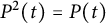 $P^{2}(t)=P(t)$
for any
 $t\geq 0$
is a consequence of its own definition, while the next result proves its invariance. This last property has not been proved in [Reference Battelli and Palmer4] and, in spite that can be deduced easily, we will prove it.
Lemma A.3 The projector
 $P(\cdot )$
is invariant, namely, it verifies the property
 $$ \begin{align*} T(t,s)P(s)=P(t)T(t,s) \quad \mathrm{for\ any}\ t,s\geq 0. \end{align*} $$
Proof Notice that
 $$ \begin{align*} T(t,s)P(s)=\left[\begin{array}{@{}cc@{}} X(t,s)P^{A}(s) & W(t,s)P^{B}(s)+X(t,s)R(s) \\ 0 & Y(t,s)P^{B}(s) \end{array}\right]. \end{align*} $$
As
 $P^{A}(\cdot )$
and
 $P^{B}(\cdot )$
are invariant projectors, we can see that the lemma follows if and only if
 $$ \begin{align*} R(t)Y(t,s)+P^{A}(t)W(t,s)=W(t,s)P^{B}(s)+X(t,s)R(s) \quad \text{for any } t,s\geq 0. \end{align*} $$
By defining
 $R_{t,s}(0):=X(t,0)R(0)Y(0,s)$
, using (A.7) and (A.8) and considering
 $t\geq s$
, we can easily deduce that
 $$ \begin{align*} R(t)Y(t,s)+P^{A}(t)W(t,s)&=\displaystyle R_{t,s}(0)+\int_{0}^{t}X(t,\tau)[C(\tau)P^{B}(\tau)-P^{A}(\tau)C(\tau)]Y(\tau,s)\,d\tau \\&\quad\displaystyle+ \int_{s}^{t}X(t,\tau)P^{A}(\tau)C(\tau)Y(\tau,s)\,d\tau \\&= \displaystyle R_{t,s}(0)+\int_{0}^{s}X(t,\tau)[C(\tau)P^{B}(\tau)-P^{A}(\tau)C(\tau)]Y(\tau,s)\,d\tau\\&\quad\displaystyle +\int_{s}^{t}X(t,\tau)C(\tau)P^{B}(\tau)Y(\tau,s)\,d\tau \\&= X(t,s)R(s)+W(t,s)P^{B}(s). \end{align*} $$
A similar identity can be deduced considering
 $t<s$
and the lemma follows.
Gathering the above results, it can be proved that the triangular system (4.1) has a (
 $\bar {K}e^{\bar {\varepsilon }s},\bar {\alpha }$
)-nonuniform exponential dichotomy on
 $\mathbb {R}_{0}^{+}$
with the above defined invariant projector
 $P(t)$
.
Lemma A.4 There exist constants
 $K_{3}\geq 1$
,
 $\alpha _{3}>0,$
and
 $\varepsilon _{3}\geq 0$
, where
 $\varepsilon _3<\alpha _3$
such that
 $$ \begin{align} \|W(t,s)P^{B}(s)+X(t,s)R(s)\|\leq K_{3}e^{-\alpha_{3}(t-s)+\varepsilon_3 s} \quad \text{for } t\geq s\geq 0. \end{align} $$
Proof In order to deduce this estimation, we will write
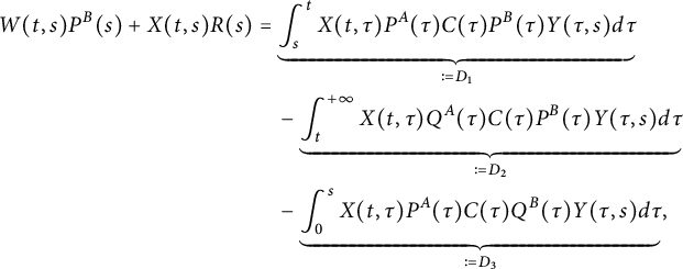 $$ \begin{align*} W(t,s)P^{B}(s)+X(t,s)R(s) &= \displaystyle \underbrace{\int_{s}^{t}X(t,\tau)P^{A}(\tau)C(\tau)P^{B}(\tau)Y(\tau,s)d\tau}_{:=D_{1}}\\&\quad -\displaystyle\underbrace{\int_{t}^{+\infty}X(t,\tau)Q^{A}(\tau)C(\tau)P^{B}(\tau)Y(\tau,s)d\tau}_{:=D_{2}}\\&\quad -\displaystyle\underbrace{\int_{0}^{s}X(t,\tau)P^{A}(\tau)C(\tau)Q^{B}(\tau)Y(\tau,s)d\tau}_{:=D_{3}}, \end{align*} $$
where
 $I_n-P^{A}(\tau )=Q^{A}(\tau )$
and
 $I_{m}-P^{B}(\tau )=Q^{B}(\tau )$
.
By using again Lemma A.1 followed by the Uniformization Lemma and recalling that
 $s\leq t$
, we have that:
 $$ \begin{align} \|D_{1}\| &\leq \displaystyle Le^{\theta s}\|C\|_{\tau,\infty}\int_{s}^{t}\|X(t,\tau)P^{A}(\tau)\|_{\tau,t}\,\|P^{B}(\tau)Y(\tau,s)\|_{s,\tau}\,d\tau \nonumber\\&\leq \displaystyle Le^{\theta s}\|C\|_{\tau,\infty}\kappa\widetilde{\kappa}\int_{s}^{t}e^{-\alpha(t-\tau)}e^{-\widetilde{\alpha}(\tau-s)}\,d\tau, \end{align} $$
 $$ \begin{align} \|D_{2}\| &\leq \displaystyle Le^{\theta s}\|C\|_{\tau, \infty}\int_{t}^{\infty}\|X(t,\tau)Q^{A}(\tau)\|_{t,\tau}\,\|P^{B}(\tau)Y(\tau,s)\|_{s,\tau}\,d\tau \nonumber\\& \leq \displaystyle Le^{\theta s}\|C\|_{\tau,\infty}\kappa\widetilde{\kappa}\int_{t}^{\infty}e^{-\alpha(\tau-t)}e^{-\widetilde{\alpha}(\tau-s)}\,d\tau, \end{align} $$
 $$ \begin{align} \|D_{3}\|&\leq \displaystyle Le^{\theta s}\|C\|_{\tau,\infty}\int_{0}^{s}\|X(t,\tau)P^{A}(\tau)\|_{\tau,t}\,\|Q^{B}(\tau)Y(\tau,s)\|_{s,\tau}\,ds \nonumber \\& \leq \displaystyle Le^{\theta s}\|C\|_{\tau,\infty}\kappa\widetilde{\kappa}\int_{0}^{s}e^{-\alpha(t-\tau)}e^{-\widetilde{\alpha}(s-\tau)}\,d\tau. \end{align} $$
As a consequence of the estimates (A.11)–(A.13) and defining
 $\kappa _{I}=\max \left \{ \kappa ,\widetilde {\kappa }\right \}$
, we have:
 $$ \begin{align*}&\|W(t,s)P^{B}(s)+X(t,s)R(s)\| \leq \displaystyle Le^{\theta s}\|C\|_{\tau,\infty}\,\kappa_{I}^{2}\int_{s}^{t}e^{-\alpha(t-\tau)}e^{-\widetilde{\alpha}(\tau-s)}d\tau \\& \qquad + \displaystyle Le^{\theta s}\|C\|_{\tau,\infty}\,\kappa_{I}^{2}\int_{t}^{+\infty}e^{-\alpha(\tau-t)}e^{-\widetilde{\alpha}(\tau-s)}d\tau + \displaystyle Le^{\theta s}\|C\|_{\tau,\infty}\,\kappa_{I}^{2}\int_{0}^{s}e^{-\alpha(t-\tau)}e^{-\widetilde{\alpha}(s-\tau)}d\tau\\& \quad \leq \displaystyle Le^{\theta s}\|C\|_{\tau,\infty}\,\kappa_{I}^{2}\cdot\left \{\left (\frac{e^{-\widetilde{\alpha}(t-s)}-e^{-\alpha(t-s)}}{\alpha-\widetilde{\alpha}}\right ) +\displaystyle \left ( \frac{e^{-\widetilde{\alpha}(t-s)}}{\alpha+\widetilde{\alpha}}\right ) +\displaystyle \left ( \frac{e^{-\alpha(t-s)}-e^{-\alpha t-\widetilde{\alpha}s}}{\alpha +\widetilde{\alpha}}\right )\right \}\\& \quad \leq \displaystyle Le^{\theta s}\|C\|_{\tau,\infty}\,\kappa_{I}^{2}\cdot\left [ \frac{1}{|\alpha-\widetilde{\alpha}|}+\frac{1}{\alpha+\widetilde{\alpha}}+\frac{1}{\alpha+\widetilde{\alpha}}\right ]e^{-\alpha_1(t-s)} \\& \quad \leq \displaystyle K_1e^{-\alpha_1(t-s)+\theta s}, \end{align*} $$
and if
 $\alpha \neq \tilde {\alpha }$
, then (A.10) is satisfied with
 $\alpha _1=\min \{\alpha ,\widetilde {\alpha }\}>\theta $
and
 $$ \begin{align*}K_1=\max\left \{1,\;\displaystyle L ||C||_{\tau,\infty}\,\kappa_{I}^{2}\cdot\left [ \frac{1}{|\alpha-\widetilde{\alpha}|}+\frac{1}{\alpha+\widetilde{\alpha}}+\frac{1}{\alpha+\widetilde{\alpha}}\right ]\right \}.\end{align*} $$
Note that, similarly as done in [Reference Battelli and Palmer4], if
 $\alpha =\widetilde {\alpha }$
, we can see that only the first term in the above brackets must be replaced by a new estimation of (A.11):
 $$ \begin{align*}\|D_{1}\| &\leq \displaystyle Le^{\theta s}\|C\|_{\tau,\infty}\kappa\widetilde{\kappa}\int_{s}^{t}e^{-\alpha(t-\tau)}e^{-\alpha(\tau-s)}\,d\tau \\&\leq \displaystyle Le^{\theta s}\|C\|_{\tau,\infty}\kappa^{2}_{I}\int_{s}^{t}e^{-\alpha(t-s)}\,d\tau\\&\leq \displaystyle Le^{\theta s}\|C\|_{\tau,\infty}\kappa^{2}_{I}(t-s)e^{-\alpha(t-s)}, \end{align*} $$
and since the estimation
 $(t-s)e^{-\gamma (t-s)}\leq \frac {1}{\gamma e}$
, for a positive
 $\gamma $
, if we have that
 $\gamma <\alpha $
and
 $\theta <\alpha -\gamma $
, then the previous inequality becomes
 $$ \begin{align*} \|D_{1}\| &\leq \displaystyle Le^{\theta s}\|C\|_{\tau,\infty}\kappa^{2}_{I}(t-s)e^{-\alpha(t-s)}\leq Le^{\theta s}\|C\|_{\tau,\infty}\kappa^{2}_{I}\frac{1}{\gamma e}e^{-(\alpha-\gamma)(t-s)}, \end{align*} $$
thus we obtain that
 $$ \begin{align*} &\|W(t,s)P^{B}(s)+X(t,s)R(s)\|\\&\quad \leq \displaystyle Le^{\theta s}\|C\|_{\tau,\infty}\kappa^{2}_{I}\frac{1}{\gamma e}e^{-(\alpha-\gamma)(t-s)}+Le^{\theta s}\|C\|_{\tau,\infty}\,\kappa_{I}^{2}\frac{1}{\alpha}e^{-\alpha(t-s)}\\&\quad \leq \displaystyle Le^{\theta s}\|C\|_{\tau,\infty}\kappa^{2}_{I}\frac{1}{\gamma }e^{-(\alpha-\gamma)(t-s)}+Le^{\theta s}\|C\|_{\tau,\infty}\,\kappa_{I}^{2}\frac{1}{\gamma}e^{-(\alpha-\gamma)(t-s)}\\&\quad \leq{K}_2e^{-\alpha_{2}(t-s)+\theta s}, \end{align*} $$
where
 $K_2=\max \left \{ 1,\; 2L||C||_{\tau ,\infty }\kappa ^{2}_{I}\frac {1}{\gamma }\right \}$
and
 $\alpha _2=\alpha -\gamma>\theta $
.
Furthermore, if we define
 $K_3:=\max \{K_1,K_2\}$
,
 $\alpha _3:=\min \{\alpha _{1},\alpha _{2}\},$
and
 $\varepsilon _{3}:=\theta $
, we can conclude the estimate (A.10).
Lemma A.5 The evolution operator of (4.1) and the projector
 $P(t)$
previously defined verify:
 $$ \begin{align*}\begin{array}{@{}rcl@{}} \left \|T(t,s)P(s)\right \|&\leq&\bar{K}e^{-\bar{\alpha}(t-s)+\bar{\varepsilon}s} \quad \mathrm{for\ any}\ t\geq s\geq 0, \end{array} \end{align*} $$
where
 $\bar {K}\geq 1$
,
 $\bar {\alpha }>0$
,
 $\bar {\varepsilon }\geq 0$
, with
 $\bar {\alpha }>\bar {\varepsilon }$
.
Proof Let us consider
 $(\xi _1,\xi _2)\in {\mathbb {R}}^{n}\times {\mathbb {R}}^{m}\setminus \{(0,0)\}$
, then we have that
 $$ \begin{align*}\left |T(t,s)P(s)\begin{pmatrix} \xi_1 \\ \xi_2 \end{pmatrix}\right |&=\left |\left[\begin{array}{@{}cc@{}} X(t,s)P^{A}(s) & W(t,s)P^{B}(s)+X(t,s)R(s) \\ 0 & Y(t,s)P^{B}(s) \end{array}\right]\begin{pmatrix} \xi_1 \\ \xi_2 \end{pmatrix}\right |,\\& = \left |\left[\begin{array}{@{}cc@{}} X(t,s)P^{A}(s)\xi_1 + (W(t,s)P^{B}(s)+X(t,s)R(s))\xi_2 \\ Y(t,s)P^{B}(s)\xi_2 \end{array}\right] \right |\\& \leq \|X(t,s)P^{A}(s)\|\cdot |\xi_1|+\\& \quad \|W(t,s)P^{B}(s)+X(t,s)R(s)\|\cdot|\xi_2|+\| Y(t,s)P^{B}(s)\|\cdot|\xi_2| \end{align*} $$
and due to the estimates (A.10) for the second summand deduced in the above lemma, the fact that
 $|\xi _i|\leq |(\xi _1,\xi _2)|$
and the estimations (A.1) and (A.2), the lemma follows easily.
The following two lemmas emulate the previous results considering the complementary projectors and
 $t\leq s$
. Allowing us to end the treatment and study of the dichotomy properties.
Lemma A.6 There exist constants
 $K_{3}\geq 1$
,
 $\alpha _{3}>0,$
and
 $\varepsilon _{3}\geq 0$
, where
 $\varepsilon _3<\alpha _3$
such that
 $$ \begin{align} \|(I_n-P^{A}(t))W(t,s)-R(t)Y(t,s)\|\leq K_{3}e^{-\alpha_3(s-t)+\varepsilon_{3}s} \quad \mathrm{for}\ s\geq t\geq 0. \end{align} $$
Proof The proof is a carbon copy of the proof of Lemma A.4 and is left for the reader.
Lemma A.7 The evolution operator of (4.1) and the projector
 $P(t)$
previously defined verify:
 $$ \begin{align*}\left \|T(t,s)[I-P(s)]\right \|&\leq\bar{K}e^{-\bar{\alpha}(s-t)+\bar{\varepsilon}s} \quad \mathrm{for\ any}\ s\geq t\geq 0, \end{align*} $$
where
 $\bar {K}\geq 1$
,
 $\bar {\alpha }>0$
,
 $\bar {\varepsilon }\geq 0$
, with
 $\bar {\alpha }>\bar {\varepsilon }$
.
Proof Let us consider
 $(\xi _1,\xi _2)\in {\mathbb {R}}^{n}\times {\mathbb {R}}^{m}\setminus \{(0,0)\}$
, then we have that
 $$ \begin{align*} \left |T(t,s)(I-P(s))\begin{pmatrix} \xi_1 \\ \xi_2 \end{pmatrix}\right |&=\left |(I-P(t))T(t,s)\begin{pmatrix} \xi_1 \\ \xi_2 \end{pmatrix}\right |\\&=\left |\left[\begin{array}{@{}cc@{}} Q^{A}(t)X(t,s) & Q^{A}(t)W(t,s)-R(t)Y(t,s) \\ 0 & Q^{B}(t)Y(t,s) \end{array}\right]\begin{pmatrix} \xi_1 \\ \xi_2 \end{pmatrix}\right |,\\&=\left |\left[\begin{array}{@{}cc@{}} Q^{A}(t)X(t,s)\xi_1 + (Q^{A}(t)W(t,s)-R(t)Y(t,s))\xi_2 \\ Q^{B}(t)Y(t,s)\xi_2 \end{array}\right] \right |\\&\leq\|Q^{A}(t)X(t,s)\|\cdot |\xi_1|+\\& \quad \|Q^{A}(t)W(t,s)-R(t)Y(t,s)\|\cdot|\xi_2|+\| Q^{B}(t)Y(t,s)\|\cdot|\xi_2| \end{align*} $$
and the lemma is a consequence of (A.14), which estimates the second summand, combined with the fact that
 $|\xi _i|\leq |(\xi _1,\xi _2)|$
.
The next result shows that the nondiagonal submatrix
 $W(t,s)$
of
 $T(t,s)$
has a property reminiscent to the forward nonuniform bounded growth.
Lemma A.8 There exist constants
 $M_{3}\geq 1$
,
 $\omega _{3}>0,$
and
 $\theta \geq 0$
such that the operator
 $W(t,s)$
, defined in (A.7), verifies
 $$ \begin{align*}\|W(t,s)\|\leq M_{3}e^{\omega_{3} (t-s)+\theta s},\quad t\geq s. \end{align*} $$
Proof Let us recall that the systems
 $\dot {x}=A(t)x$
and
 $\dot {y}=B(t)y$
have a forward nonuniform bounded growth on
 ${\mathbb {R}}_{0}^{+}$
described in (A.3). By using Lemma A.1, where
 $Z(\tau )=I_{n}$
and
 $V(\tau )=I_{m}$
, combined with (A.4) which arises from the Uniformization Lemma, we can see that when
 $t\geq s\geq 0$
:
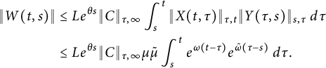 $$ \begin{align*} \|W(t,s)\|&\leq\displaystyle Le^{\theta s}\|C\|_{\tau,\infty}\int_{s}^{t}\|X(t,\tau)\|_{\tau,t} \|Y(\tau,s)\|_{s,\tau}\; d\tau\\&\leq Le^{\theta s}\|C\|_{\tau,\infty}\mu\tilde{\mu} \displaystyle\int_{s}^{t}e^{\omega (t-\tau)}e^{\tilde{\omega}(\tau-s)}\; d\tau. \end{align*} $$
Here, we have two cases. The first one is when
 $\omega \neq \tilde {\omega }$
, then if
 $\mu _{I}=\max \{\mu ,\tilde {\mu }\}$
:
 $$ \begin{align*} \|W(t,s)\|&\leq Le^{\theta s}\|C\|_{\tau,\infty}\mu_{I}^{2} e^{\omega t-\tilde{\omega} s}\displaystyle\int_{s}^{t}e^{(\omega-\tilde{\omega})\tau}\; d\tau\\&=\displaystyle Le^{\theta s}\|C\|_{\tau,\infty}\mu_{I}^{2} \frac{1}{|\tilde{\omega}-\omega|}\left [e^{\tilde{\omega} (t-s)}-e^{\omega(t-s)}\right ]\\&\leq\displaystyle M_1 e^{\omega_1(t-s)+\theta s}, \end{align*} $$
where
 $$ \begin{align*}M_1=\max\left \{ 1, \displaystyle L\|C\|_{\tau,\infty}\mu_{I}^{2} \frac{2}{|\tilde{\omega}-\omega|}\right \}\quad \text{and}\quad \omega_{1}=\max\{\omega,\tilde{\omega}\}.\end{align*} $$
The second case is when
 $\omega =\tilde {\omega }$
, then
 $$ \begin{align*} \|W(t,s)\|&\leq Le^{\theta s}\|C\|_{\tau,\infty}\mu_{I}^{2}\displaystyle\int_{s}^{t}e^{\omega(t-s)}\; d\tau\\&\leq\displaystyle Le^{\theta s}\|C\|_{\tau,\infty}\mu_{I}^{2} e^{\omega(t-s)}e^{(t-s)}\\&\leq\displaystyle M_2 e^{\omega_{2}(t-s)+\theta s}, \end{align*} $$
where
 $$ \begin{align*}M_2=\max \left \{ 1, L\|C\|_{\tau,\infty}\mu_{I}^{2} \right \}\quad \text{and}\quad \omega_{2}=\omega+1.\end{align*} $$
Based on the two cases analyzed, we can conclude that
 $$ \begin{align} \|W(t,s)\|\leq Me^{\omega_{3} (t-s)+\theta s},\quad t\geq s, \end{align} $$
where
 $$ \begin{align*}M_3=\max \left \{M_1, M_2\right \}\quad \text{and}\quad \omega_{3}=\max\{\omega_1,\omega_2\}.\\[-33pt]\end{align*} $$
The last result shows that the evolution operator associated with the upper triangular system (2.1) has the property of forward
 $(\overline {M}e^{\overline {\theta }s},\overline {\omega })$
-nonuniform bounded growth.
Lemma A.9 The evolution operator of (4.1) verifies:
 $$ \begin{align*}\left \|T(t,s)\right \|\leq\bar{M}e^{\bar{\omega}(t-s)+\bar{\theta}s} \quad \mathrm{for\ any}\ t\geq s\geq 0, \end{align*} $$
where
 $\bar {M}\geq 1$
,
 $\bar {\omega }>0$
, and
 $\bar {\theta }\geq 0$
.
Proof If we consider
 $(\xi _1,\xi _2)\in {\mathbb {R}}^{n}\times {\mathbb {R}}^{m}\setminus \{(0,0)\}$
, then we have that
 $$ \begin{align*} \left |T(t,s)\begin{pmatrix} \xi_1 \\ \xi_2 \end{pmatrix}\right |&=\left |\left[\begin{array}{@{}cc@{}} X(t,s) & W(t,s) \\ 0 & Y(t,s) \end{array}\right]\begin{pmatrix} \xi_1 \\ \xi_2 \end{pmatrix}\right |,\\&=\left |\left[\begin{array}{@{}cc@{}} X(t,s)\xi_1 + W(t,s)\xi_2 \\ Y(t,s)\xi_2 \end{array}\right] \right |\\&\leq\|X(t,s) \|\cdot |\xi_1|+\\& \quad \|W(t,s)\|\cdot|\xi_2|+\| Y(t,s)\|\cdot|\xi_2| \end{align*} $$
and due to the estimation (A.15), the fact that
 $|\xi _i|\leq |(\xi _1,\xi _2)|$
and both estimations in (A.3), we can ensure that for
 $t\geq s$
:
 $$ \begin{align*}\|T(t,s)\|\leq \bar{M}e^{\bar{\theta} s}e^{\bar{\omega}(t-s)}.\\[-33pt] \end{align*} $$
A.2 End of proof of Theorem 1
Firstly, Lemmas A.3, A.5, and A.7 imply that the triangular system (4.1) has a
 $(\bar {K}e^{\bar {\varepsilon }s},\bar {\alpha })$
-nonuniform exponential dichotomy in
 $\mathbb {R}_{0}^{+}$
.
Secondly, Lemma A.9 says that the system (4.1) has the property of forward
 $(\bar {M}e^{\bar {\theta }s},\bar { \omega })$
-nonuniform bounded growth and the theorem follows.
Remark A.1 A meticulous reading of this Appendix shows that the property of forward nonuniform bounded growth is fundamental in several steps of the proof:
-
a) Is a necessary condition in order to use the Uniformization Lemma, which ensures the existence of a continuous family norms
$\{|\cdot |_{t}\}$
verifying the inequality
${|x|_{t}\leq L_{2}(t)|x|}$
. The forward nonuniform bounded growth property is a required tool in order to obtain explicit estimations for
$L_{2}(\cdot )$
and (A.5). -
b) The constants
$\ell $
and
$\tilde {\ell }$
are necessary to deduce (A.5) and (A.6), these identities are immersed in Lemma A.1, which is the main key to deduce several estimations around the proof. -
c) The previous facts also show that the boundedness properties of
$\|C(\tau )\|_{\tau ,\tau }$
involve estimations based on the forward nonuniform bounded growth property.




We point out that in [Reference Tien, Nhien and Chien36], the property of forward nonuniform bounded growth is not considered neither in the statement of Uniformization Lemma (Lemma 2.2 in [Reference Tien, Nhien and Chien36]) nor in the statement of Theorem 2.3.
Acknowledgements
The authors acknowledge the anonymous reviewer by his helpful comments and suggestions which improved this article.



