1 Introduction
Density fronts, which are defined as regions of large density gradients, are features ubiquitous in the ocean and the atmosphere. For instance western boundary currents, such as the Gulf Stream and the Kuroshio, are the site of large-scale meanders resulting in mesoscale eddies, which are typically 10–100 km in horizontal length scale with Rossby numbers smaller than unity. These eddies draw energy from the geostrophic flow by converting potential into kinetic energy (Gnanadesikan et al. Reference Gnanadesikan, Slater, Swathi and Vallis2005; Wolfe et al. Reference Wolfe, Cessi, McClean and Maltrud2008; Thomas et al. Reference Thomas, Taylor, Ferrari and Joyce2013; Zemskova, White & Scotti Reference Zemskova, White and Scotti2015). The kinetic energy in these eddies can in turn dissipate through submesoscale instabilities (typically smaller than 1 km), in addition to other mechanisms such as bottom drag, but the transient dynamics of the submesoscale instabilities is still not completely understood (Thomas et al. Reference Thomas, Taylor, Ferrari and Joyce2013; Stamper & Taylor Reference Stamper and Taylor2017). These submesoscale processes enhance the vertical transport in the upper ocean and have an impact on phytoplankton and the biological pump, and their energetics need to be explored further (Taylor & Ferrari Reference Taylor and Ferrari2011; Omand et al. Reference Omand, DAsaro, Lee, Perry, Briggs, Cetinić and Mahadevan2015; Sarkar et al. Reference Sarkar, Pham, Ramachandran, Nash, Tandon, Buckley, Lotliker and Omand2016; Brannigan et al. Reference Brannigan, Marshall, Naveira Garabato, Nurser and Kaiser2017; Ramachandran et al. Reference Ramachandran, Tandon, Mackinnon, Lucas, Pinkel, Waterhouse, Nash, Shroyer, Mahadevan and Weller2018).
Small-scale perturbations have also been identified as an energy source for geophysical shear flows with undisturbed background state, such as the Earth’s midlatitude jets (Farrell & Ioannou Reference Farrell and Ioannou1993c) and zonal winds in gaseous planets (Vasavada & Showman Reference Vasavada and Showman2005), with a particular interest on the effect of these perturbations on cyclogenesis. However, the stability and dynamics of the fronts where small-scale instabilities are confined in narrow regions have received less attention than the small aspect ratio and hydrostatic counterpart. Larger aspect ratios are particularly common in hurricane boundary layers (Ellis & Businger Reference Ellis and Businger2010; Foster Reference Foster2013) and tornados (Nolan et al. Reference Nolan, Dahl, Bryan and Rotunno2017). This confinement reduces the spatial support for large baroclinic geostrophic instabilities where non-hydrostatic effects are known to damp geostrophic-type motions (Stone Reference Stone1970). Hence ageostrophic-type modes, characterized by short wavelength and critical regions associated with intense shear, are expected to play a dominant role in the submesoscale transition process.
The role of submesoscale instabilities was first identified by Solberg (Reference Solberg1936) in the case of symmetric modes and later by Eady (Reference Eady1949) for baroclinic modes and finally by Chandrasekhar (Reference Chandrasekhar1961) for Kelvin–Helmholtz-type waves. The stability of fronts and normal growth rates of instabilities were extensively analysed using asymptotic theory for a linear thermal wind shear (Stone Reference Stone1966, Reference Stone1970, Reference Stone1971). In general, baroclinic instabilities include any instabilities that arise in a rotating fluid which is stratified due to horizontal density gradients. Here, to be consistent with Stone’s work and subsequent analyses done in his footsteps (e.g. Molemaker, McWilliams & Yavneh Reference Molemaker, McWilliams and Yavneh2005; Stamper & Taylor Reference Stamper and Taylor2017), we refer to baroclinic instabilities as those that occur independently of perturbations in the meridional direction and draw energy from potential energy of the flow to distinguish them from symmetric modes that are independent of zonal perturbations and draw energy from the kinetic energy field.
A geostrophic current is symmetrically unstable when its potential vorticity has the opposite sign of local Coriolis parameter (Thomas et al. Reference Thomas, Taylor, Ferrari and Joyce2013), but the unstable modal growth rate is non-zero only when the Richardson number  $Ri<1$ for a basic state in thermal wind shear balance with no vertical vorticity (Stone Reference Stone1966). Baroclinic instabilities are divided into geostrophic and ageostrophic types. While these instabilities are technically geostrophic only for
 $Ri\gg 1$ as described by Eady (Reference Eady1949), we again follow Stone’s convention in referring to any baroclinic instabilities at any value of
 $Ri$ with large wavelength and large modal growth rates as geostrophic, while the ageostrophic ones occur at much smaller length scales and have smaller growth rates. The geostrophic and ageostrophic instabilities also have different structures of the eigenspectra, as will be discussed in detail in §§ 2.3 and 4.1. In particular, the geostrophic-type instabilities have only one eigenmode with the largest real part of eigenvalue while the ageostrophic-type instabilities have two eigenmodes with the largest equal real part but different imaginary parts of the eigenvalue. Ageostrophic modes have been previously overlooked, but it has been shown that they may play an important role in restratification of ocean mixed layer (Boccaletti, Ferrari & Fox-Kemper Reference Boccaletti, Ferrari and Fox-Kemper2007) and loss of balance (Molemaker et al. Reference Molemaker, McWilliams and Yavneh2005).
Heifetz & Farrell (Reference Heifetz and Farrell2003) generalized the notion of stability in baroclinic shear flows in the large Richardson (strongly stratified) regime using a formulation based on primitive equations. In a second study, Heifetz & Farrell (Reference Heifetz and Farrell2007) showed that the non-normal coupling between stable (Rossby- or inertio-gravity) waves and unstable geostrophic modes results in energy gain which exceeds that provided by the modal growth alone in the hydrostatic limit. Heifetz & Farrell (Reference Heifetz and Farrell2008) also extended their analysis to symmetric modes and showed the optimal transient growth exceeding that predicted by normal symmetric mode analysis and yielding potentially a much faster generation of slantwise convection. However, the extra gains that they report are at most a factor two, which is relatively small compared to the extra optimal gain observed for the geostrophic and ageostrophic type modes. For all cases, this shear-driven transient energy growth is known to be the bypass transition to turbulence, which in turn was developed by the hydrodynamic community for asymptotically stable shear flows by Schmid & Henningson (Reference Schmid and Henningson2012). Finite amplitude perturbations that undergo transient growth may reach an amplitude that is sufficiently large to allow positive feedback through nonlinear interactions that amplify the growing disturbances. In the present study, we consider a generalization of Heifetz & Farrell (Reference Heifetz and Farrell2003, Reference Heifetz and Farrell2007) by taking it to the non-hydrostatic limit commonly found during frontogenesis that induces finite thicknesses of the front leading to geostrophic shear with large aspect ratios.
While oceanic flows are generally characterized by small aspect ratios (defined here as the ratio of the vertical to horizontal length scales), commonly found between  $10^{-1}$ and
 $10^{-3}$, atmospheric flows can have aspect ratios of the order of unity (Nolan et al. Reference Nolan, Dahl, Bryan and Rotunno2017) and the non-hydrostatic effects may be important. Stone (Reference Stone1971) theoretically derived the non-hydrostatic effects on the most unstable modes for the linear thermal wind shear framework. This work found that the temporal energy growth rates are progressively suppressed as the aspect ratio increases for all instability types. However, it is possible that for a short term, the energy gain is not as affected by non-hydrostatic conditions. The latter may even provide a route for the transient growth of perturbations which will be one of the main focuses of this study. For instance, the energy gain of short-lived near-surface streaks in the hurricane boundary layer that enhance wind speed and vertical transport could be attributed to such non-normal transient growth dynamics (Drobinski & Foster Reference Drobinski and Foster2003).
Unstratified simple shear flows such as plane Couette or plane Poiseuille configurations are known to be subject to two types of transient growth phenomena. In his original work, Orr (Reference Orr1907) showed that in the case of a simple inviscid parallel shear flow, perturbations with a non-zero streamwise wavenumber could produce transient growth through the kinematic deformation of the perturbation vorticity by the baseflow advection and shear. Later, Farrell & Ioannou (Reference Farrell and Ioannou1993a) derived an analytic solution for the Orr temporal growth rate, for two-dimensional perturbations in a constant, unstratified linear shear. Ellingsen & Palm (Reference Ellingsen and Palm1975) recognized that a finite disturbance independent of the streamwise coordinate (i.e. with a spanwise wavenumber with respect to the shear) may lead to instability of linear flow, even though the basic velocity does not possess an inflection point. This mechanism, later denoted as lift-up effect, is a key process in the laminar–turbulent transition in shear flows and in fully developed turbulence (Brandt Reference Brandt2014).
The energy growth mechanisms in stratified and rotating sheared flows have been addressed in several previous works, such as Farrell & Ioannou (Reference Farrell and Ioannou1993b), Bakas & Farrell (Reference Bakas and Farrell2009a,Reference Bakas and Farrellb) and Park, Billant & Baik (Reference Park, Billant and Baik2017). These works identified several mechanisms responsible for the energy growth that vary depending on the configuration of the background flow and the stratification. In particular, Park et al. (Reference Park, Billant and Baik2017) noted that there exist two mechanisms types for transient energy growth analogous to the lift up and the Orr mechanisms in homogeneous fluids but with the additional effect of density perturbations. In this work, we explore the transient energy growth mechanisms for different Richardson number regimes over a range of zonal and meridional wavenumbers with respect to the height or depth of the front. In particular, we assess the additional contribution of the energy transfer from the background flow to the perturbations through the wave reflection off the domain boundaries and critical layers.
The local stability properties and loss of balance induced by baroclinic modes and their dependence on Rossby number in thermal wind balance was first computed numerically using a finite difference matrix-type approach to this eigenvalue problem rather than an iterative shooting method with an initial eigenvalue guess by Molemaker et al. (Reference Molemaker, McWilliams and Yavneh2005). They showed that they could capture the instability modes predicted by Stone (Reference Stone1970) and that these modes explained in part how a highly balanced large-scale circulation may dissipate energy through a local forward energy cascade into unbalanced motions. Nakamura (Reference Nakamura1988) showed that ageostrophic modes are identified within the inertial critical layer which is sustained by the resonance between one of the boundary modes and the inertial gravity waves. The latter observation implies that computing the eigenspectrum in the non-hydrostatic and inviscid limit based on the Molemaker et al. (Reference Molemaker, McWilliams and Yavneh2005) formulation may lead to spurious or unresolved eigenfunctions in the critical layers. The computation of optimal initial disturbances and optimal energy gain using a singular value decomposition method described by Schmid & Brandt (Reference Schmid and Brandt2014) requires the interaction of all modes, not only modes with non-zero energy growth rate. As some of the obtained eigenfunctions may be spurious or unresolved, it is necessary to determine the criteria for the selection of the only physical and resolved eigenmodes appropriate for the these computations.
In the present paper, we start from a one-dimensional finite difference approximation of the linearized Euler equation for a flow in thermal wind balance following Stone (Reference Stone1966, Reference Stone1970, Reference Stone1971), and compute optimal energy growth for a range of Richardson number values as well as wavenumbers in both horizontal directions. We overcome the problem of critical layers by performing a careful selection of the appropriate modes used in the Galerkin-type projection to compute the optimal initial disturbance. In particular, we provide selection criteria that allow for discarding of the spurious eigenfunctions. The energy budget and nonlinear development of the optimal initial conditions are computed using three-dimensional non-hydrostatic direct numerical simulations (DNS) of the Navier–Stokes equations.
The rest of the paper is organized as follows: § 2 presents the numerical methods and set-up of the problem, transient growth and the selection criteria for the eigenfunctions are explained in § 3. Results for the linear optimal dynamics are summarized in § 4, whereas three-dimensional simulations are given in § 5 and conclusions are drawn in § 6.
2 Theoretical formulation
2.1 Problem set-up
The present formulation is based on Stone (Reference Stone1970, Reference Stone1971) and considers the dynamics of a non-hydrostatic and rotating inviscid fluid in the Boussinesq limit where  $f$ is the Coriolis frequency. The governing conservation equations for the zonal velocity
 $\hat{u}$, meridional velocity
 $\hat{v}$, vertical velocity
 ${\hat{w}}$, hydrodynamic pressure
 $\hat{p}^{\prime }=\hat{p}/\unicode[STIX]{x1D70C}_{0}$ and buoyancy
 $\hat{b}=-g(\hat{\unicode[STIX]{x1D70C}}-\hat{\unicode[STIX]{x1D70C}_{0}})/\hat{\unicode[STIX]{x1D70C}_{0}}$ (where
 $g$ is the gravitational acceleration) are
 $$\begin{eqnarray}\frac{\text{D}\hat{\boldsymbol{u}}}{\text{D}t}+f\boldsymbol{e}_{\boldsymbol{z}}\times \hat{\boldsymbol{u}}=-\unicode[STIX]{x1D735}\hat{p}^{\prime }+\hat{b}\boldsymbol{e}_{\boldsymbol{ z}},\quad \unicode[STIX]{x1D735}\boldsymbol{\cdot }\hat{\boldsymbol{u}}=0,\quad \frac{\text{D}\hat{b}}{\text{D}t}=0,\end{eqnarray}$$
where  $\text{D}/\text{D}\hat{t}=\unicode[STIX]{x2202}/\unicode[STIX]{x2202}\hat{t}+\hat{\boldsymbol{u}}\boldsymbol{\cdot }\unicode[STIX]{x1D735}$, and
 $\boldsymbol{e}_{\boldsymbol{z}}$ is the vertical unit vector positive upward. The domain is unbounded in the
 $\hat{x}$ (zonal) and
 ${\hat{y}}$ (meridional) directions with solid vertical boundaries at
 $\hat{z}=[0,H]$, where we impose the boundary condition
 ${\hat{w}}=0$. The base buoyancy field has constant vertical stratification and gradient in the meridional direction. The base state has zero meridional and vertical velocities and the zonal velocity has a constant vertical shear in a thermal wind balance (Vallis Reference Vallis2017).
The governing equations (2.1) are non-dimensionalized following the time and length scales prescribed in Stone (Reference Stone1971) such that
 $$\begin{eqnarray}\left.\begin{array}{@{}c@{}}(x,y)={\displaystyle \frac{f(\hat{x},{\hat{y}})}{u_{0}}},\quad z={\displaystyle \frac{\hat{z}}{H}},\quad t=\hat{t}f,\\ (u,v)={\displaystyle \frac{(\hat{u} ,\hat{v})}{u_{0}}},\quad w={\displaystyle \frac{{\hat{w}}}{fH}},\quad p={\displaystyle \frac{\hat{p}^{\prime }}{N^{2}H^{2}}},\quad b={\displaystyle \frac{\hat{b}}{HN^{2}}},\end{array}\right\}\end{eqnarray}$$
where  $u_{0}$ is the maximum zonal velocity and
 $N=\unicode[STIX]{x2202}b/\unicode[STIX]{x2202}z$ is the Brunt–Väisälä frequency. The base state variables in the non-dimensional form become
 $$\begin{eqnarray}V=W=0,\quad U=z,\quad \text{and}\quad B=z-\frac{y}{Ri},\end{eqnarray}$$
where  $Ri=H^{2}N^{2}/u_{0}^{2}$ is the Richardson number. The non-dimensionalized system (2.1) once linearized around the base state becomes
 $$\begin{eqnarray}\displaystyle & \displaystyle \frac{\unicode[STIX]{x2202}u}{\unicode[STIX]{x2202}t}+U\frac{\unicode[STIX]{x2202}u}{\unicode[STIX]{x2202}x}+w\frac{\unicode[STIX]{x2202}U}{\unicode[STIX]{x2202}z}-v+Ri\frac{\unicode[STIX]{x2202}p}{\unicode[STIX]{x2202}x}=0, & \displaystyle\end{eqnarray}$$
 $$\begin{eqnarray}\displaystyle & \displaystyle \frac{\unicode[STIX]{x2202}v}{\unicode[STIX]{x2202}t}+U\frac{\unicode[STIX]{x2202}v}{\unicode[STIX]{x2202}x}+u+Ri\frac{\unicode[STIX]{x2202}p}{\unicode[STIX]{x2202}y}=0, & \displaystyle\end{eqnarray}$$
 $$\begin{eqnarray}\displaystyle & \displaystyle \unicode[STIX]{x1D6FF}^{2}\left(\frac{\unicode[STIX]{x2202}w}{\unicode[STIX]{x2202}t}+U\frac{\unicode[STIX]{x2202}w}{\unicode[STIX]{x2202}x}\right)-Ri\,b+Ri\frac{\unicode[STIX]{x2202}p}{\unicode[STIX]{x2202}z}=0, & \displaystyle\end{eqnarray}$$
 $$\begin{eqnarray}\displaystyle & \displaystyle \frac{\unicode[STIX]{x2202}b}{\unicode[STIX]{x2202}t}+U\frac{\unicode[STIX]{x2202}b}{\unicode[STIX]{x2202}x}-\frac{v}{Ri}+w=0, & \displaystyle\end{eqnarray}$$
 $$\begin{eqnarray}\displaystyle & \displaystyle \frac{\unicode[STIX]{x2202}u}{\unicode[STIX]{x2202}x}+\frac{\unicode[STIX]{x2202}v}{\unicode[STIX]{x2202}y}+\frac{\unicode[STIX]{x2202}w}{\unicode[STIX]{x2202}z}=0, & \displaystyle\end{eqnarray}$$
 $\unicode[STIX]{x1D6FF}=fH/u_{0}$ is a measure of the aspect ratio
 $\unicode[STIX]{x1D706}=H/L$ divided by the Rossby number
 $Ro=u_{0}/fL$ as the horizontal length scale is
 $L=u_{0}/f$. Note that the deviation from hydrostatic equilibrium is determined by the value
 $\unicode[STIX]{x1D6FF}^{2}/Ri=f^{2}/N^{2}$ and provides a rescaling of the vertical velocity
 $w$ and the buoyancy perturbation
 $b$ with respect to the horizontal components
 $(u,v,p)$ in the case of finite length scales. This number also corresponds to the squared aspect ratio
 $\unicode[STIX]{x1D706}$ when choosing
 $L=NH/f$ as a horizontal length scale as in Molemaker et al. (Reference Molemaker, McWilliams and Yavneh2005).
2.2 Stability analysis
The solution for the stability is sought in terms of linear perturbation variables, denoted by the superscript  $(\,\tilde{\;}\,)$ such that
 $$\begin{eqnarray}(u,v,w,p,b)=(\tilde{u} (z),\tilde{v}(z),\tilde{w}(z),\tilde{p}(z),\tilde{b}(z))\text{e}^{\text{i}(\unicode[STIX]{x1D714}t+\unicode[STIX]{x1D6FC}x+\unicode[STIX]{x1D6FD}y)},\end{eqnarray}$$
where  $\unicode[STIX]{x1D6FC}$ and
 $\unicode[STIX]{x1D6FD}$ are zonal and meridional wavenumbers, respectively and where
 $\unicode[STIX]{x1D714}$ is the eigenvalue. Substituting the ansatz (2.5) in system (2.4), the eigenvalue problem consists of a coupled system of ordinary differential equations, expressed in terms of
 $z$-dependence only for the perturbation variables
 $(\tilde{u} ,\tilde{v},\tilde{w},\tilde{p},\tilde{b})$ with
 $$\begin{eqnarray}\displaystyle & \displaystyle \text{i}(\unicode[STIX]{x1D714}+\unicode[STIX]{x1D6FC}U)\tilde{u} -\tilde{v}+\tilde{w}+\text{i}\unicode[STIX]{x1D6FC}Ri\,\tilde{p}=0, & \displaystyle\end{eqnarray}$$
 $$\begin{eqnarray}\displaystyle & \displaystyle \tilde{u} +\text{i}(\unicode[STIX]{x1D714}+\unicode[STIX]{x1D6FC}U)\tilde{v}+\text{i}\unicode[STIX]{x1D6FD}Ri\,\tilde{p}=0, & \displaystyle\end{eqnarray}$$
 $$\begin{eqnarray}\displaystyle & \displaystyle \text{i}\unicode[STIX]{x1D6FF}^{2}(\unicode[STIX]{x1D714}+\unicode[STIX]{x1D6FC}U)\tilde{w}+Ri{\displaystyle \frac{\text{d}\tilde{p}}{\text{d}z}}-Ri\,\tilde{b}=0, & \displaystyle\end{eqnarray}$$
 $$\begin{eqnarray}\displaystyle & \displaystyle -\frac{\tilde{v}}{Ri}+\tilde{w}+\text{i}(\unicode[STIX]{x1D714}+\unicode[STIX]{x1D6FC}U)\tilde{b}=0, & \displaystyle\end{eqnarray}$$
 $$\begin{eqnarray}\displaystyle & \displaystyle \text{i}\unicode[STIX]{x1D6FC}\tilde{u} +\text{i}\unicode[STIX]{x1D6FD}\tilde{v}+\frac{\text{d}\tilde{w}}{\text{d}z}=0. & \displaystyle\end{eqnarray}$$
 $\tilde{w}$, buoyancy
 $\tilde{b}$ and vertical vorticity
 $\tilde{\unicode[STIX]{x1D702}}\equiv \unicode[STIX]{x2202}v/\unicode[STIX]{x2202}x-\unicode[STIX]{x2202}u/\unicode[STIX]{x2202}y=\text{i}\unicode[STIX]{x1D6FC}\tilde{v}-\text{i}\unicode[STIX]{x1D6FD}\tilde{u}$ that read
 $$\begin{eqnarray}\displaystyle & \displaystyle \text{i}\unicode[STIX]{x1D714}\left({\displaystyle \frac{\text{d}^{2}}{\text{d}z^{2}}}-k^{2}\unicode[STIX]{x1D6FF}^{2}\right)\tilde{w}=-\text{i}\unicode[STIX]{x1D6FC}U\left(\frac{\text{d}^{2}}{\text{d}z^{2}}-k^{2}\unicode[STIX]{x1D6FF}^{2}\right)\tilde{w}-k^{2}Ri\,\tilde{b}+\frac{\text{d}\tilde{\unicode[STIX]{x1D702}}}{\text{d}z}, & \displaystyle\end{eqnarray}$$
 $$\begin{eqnarray}\displaystyle & \displaystyle \text{i}\unicode[STIX]{x1D714}\tilde{b}=\left(\frac{\text{i}\unicode[STIX]{x1D6FD}}{k^{2}Ri}\frac{\text{d}}{\text{d}z}-1\right)\tilde{w}-\text{i}\unicode[STIX]{x1D6FC}U\tilde{b}+\frac{\text{i}\unicode[STIX]{x1D6FC}}{k^{2}Ri}\tilde{\unicode[STIX]{x1D702}}, & \displaystyle\end{eqnarray}$$
 $$\begin{eqnarray}\displaystyle & \displaystyle \text{i}\unicode[STIX]{x1D714}\tilde{\unicode[STIX]{x1D702}}=-\left(\text{i}\unicode[STIX]{x1D6FD}+\frac{\text{d}}{\text{d}z}\right)\tilde{w}-\text{i}\unicode[STIX]{x1D6FC}U\tilde{\unicode[STIX]{x1D702}}, & \displaystyle\end{eqnarray}$$
 $k^{2}=\unicode[STIX]{x1D6FC}^{2}+\unicode[STIX]{x1D6FD}^{2}$, and which in matrix form become
 $$\begin{eqnarray}\unicode[STIX]{x1D714}J\boldsymbol{q}=L\boldsymbol{q},\end{eqnarray}$$
where  $\boldsymbol{q}=[\tilde{w},\tilde{b},\tilde{\unicode[STIX]{x1D702}}]$ and
 $\unicode[STIX]{x1D645}$ and
 $\unicode[STIX]{x1D647}$ are matrices given by
 $$\begin{eqnarray}\unicode[STIX]{x1D645}=\left[\begin{array}{@{}ccc@{}}D^{2}-k^{2}\unicode[STIX]{x1D6FF}^{2} & 0 & 0\\ 0 & I & 0\\ 0 & 0 & I\end{array}\right]\end{eqnarray}$$
and
 $$\begin{eqnarray}\unicode[STIX]{x1D647}=\left[\begin{array}{@{}ccc@{}}-\unicode[STIX]{x1D6FC}U(D^{2}-k^{2}\unicode[STIX]{x1D6FF}^{2}) & \text{i}Ri\,k^{2} & -\text{i}D\\ {\displaystyle \frac{\unicode[STIX]{x1D6FD}D}{Ri\,k^{2}}}+\text{i} & -\unicode[STIX]{x1D6FC}U & {\displaystyle \frac{\unicode[STIX]{x1D6FC}}{Ri\,k^{2}}}\\ \text{i}D-\unicode[STIX]{x1D6FD} & 0 & -\unicode[STIX]{x1D6FC}U\end{array}\right]\end{eqnarray}$$
and where  $D=\text{d}/\text{d}z$ and the boundary conditions
 $$\begin{eqnarray}\tilde{w}|_{z=0,1}=0.\end{eqnarray}$$
The coupled eigenvalue problem (2.7) is discretized finally using second-order finite differences with  $N_{z}=1000$ equally spaced grid points along the vertical direction
 $z$ as in Molemaker et al. (Reference Molemaker, McWilliams and Yavneh2005), giving rise to a matrix-type eigenvalue problem that can later be used to perform transient growth analysis (Schmid & Henningson Reference Schmid and Henningson2012).
In the next subsection, we analyse the asymptotic properties of the eigenvalue problem originally formulated in Stone (Reference Stone1971) for the vertical velocity only, equivalent to the system (2.7a–c). In particular, we carry out dispersion relation analyses for this particular system to identify and then separate the resolved from the spurious modes.
2.3 Eigenvalue spectrum and mode selection
In his original work, Stone (Reference Stone1971) showed that (2.6) could be combined into a single equation for the vertical velocity which writes
 $$\begin{eqnarray}(1-\unicode[STIX]{x1D719}^{2})\frac{\text{d}^{2}w}{\text{d}z^{2}}-2\left(\frac{\unicode[STIX]{x1D6FC}}{\unicode[STIX]{x1D719}}-\text{i}\unicode[STIX]{x1D6FD}\right)\frac{\text{d}w}{\text{d}z}-\left(Ri(\unicode[STIX]{x1D6FC}^{2}+\unicode[STIX]{x1D6FD}^{2})-(\unicode[STIX]{x1D6FC}^{2}+\unicode[STIX]{x1D6FD}^{2})\unicode[STIX]{x1D6FF}^{2}\unicode[STIX]{x1D719}^{2}+\frac{2\text{i}\unicode[STIX]{x1D6FC}\unicode[STIX]{x1D6FD}}{\unicode[STIX]{x1D719}}\right)w=0,\end{eqnarray}$$
where  $\unicode[STIX]{x1D719}(z)=\unicode[STIX]{x1D714}+\unicode[STIX]{x1D6FC}U(z)$, and used asymptotic arguments to compute approximations of both geostrophic and ageostrophic modes. As can be readily seen from the terms containing
 $\unicode[STIX]{x1D719}$ in (2.12), the eigenvalue problem turns out to have multiple critical points that occur at
 $\unicode[STIX]{x1D719}(z)=[-1,0,1]$. Therefore, one would expect to observe different branches associated with each critical solution in the eigenspectrum. This was previously observed by several authors (Nakamura Reference Nakamura1988; Heifetz & Farrell Reference Heifetz and Farrell2003) who already suggested that certain branches, associated with particular physical phenomena, could be removed. More precisely, Heifetz & Farrell (Reference Heifetz and Farrell2003) used the Nakamura (Reference Nakamura1988) analysis to identify continuous branches associated with critical layers. Heifetz & Farrell (Reference Heifetz and Farrell2003) chose to reintroduce viscosity to stabilize these eigenfunctions and smooth the jump across the critical points. In their subsequent study, Heifetz & Farrell (Reference Heifetz and Farrell2007) show in their figure 1 that there exists a strong non-orthogonality that is likely to deteriorate when increasing the number of discretization points in the matrix used to solve the eigenvalue problem. The interactions between modes that are orthogonal to each other do not contribute to the energy of the system, whereas non-orthogonal modes make additional contributions to the energy gain. The importance of this orthogonality condition between modes was reinforced by the study of Molemaker et al. (Reference Molemaker, McWilliams and Yavneh2005) who also mentioned that a large number of discretization points were necessary to obtain accurate eigenvalues. In addition, Heifetz & Farrell (Reference Heifetz and Farrell2003) noted that it was necessary to remove modes that do not contribute to transient growth but appear in the solution as non-fully resolved marginally oscillatory modes. These modes, also known as Poincaré waves (cf. Heifetz & Farrell Reference Heifetz and Farrell2003, pp. 59–60), are the inertio-gravity waves in the absence of shear which are pure harmonic waves.
In this study, we have chosen not to reintroduce viscosity. Instead, we derive dispersion relations for both inertia–gravity waves and the rotational singular modes, associated with the critical layers at  $\unicode[STIX]{x1D719}(z)=[-1,0,1]$, which allows for computing of the ranges of their
 $(\unicode[STIX]{x1D714}_{r},\unicode[STIX]{x1D714}_{i})$ values. Based on these ranges, it is possible to select the appropriate subspace of eigenmodes from the full eigenspectra to compute the transient growth rates.
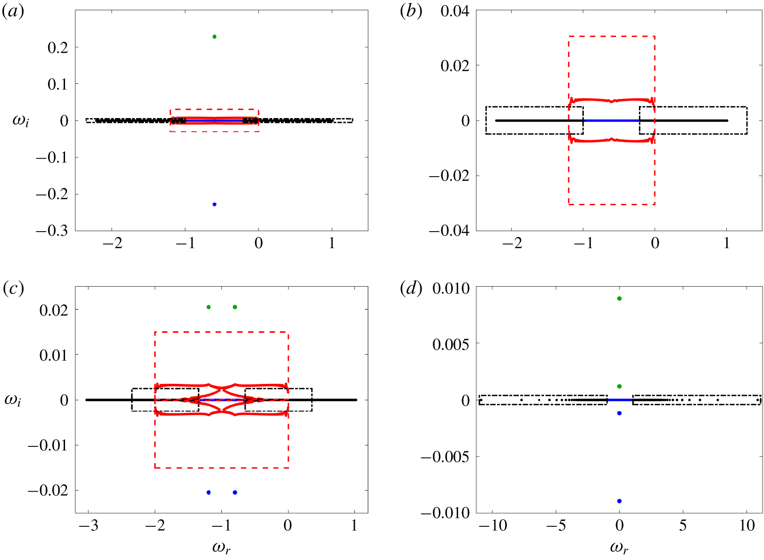
Schematic of eigenspectra obtained by solving the eigenvalue problem (2.7) for  $Ri=0.92$,
 $\unicode[STIX]{x1D6FF}=0$ and (a) geostrophic mode
 $\unicode[STIX]{x1D6FC}=1.2$,
 $\unicode[STIX]{x1D6FD}=0$; (b) close up view of the eigenspectrum from (a) around the real axis; (c) ageostrophic mode
 $\unicode[STIX]{x1D6FC}=2$,
 $\unicode[STIX]{x1D6FD}=0$; (d) symmetric mode
 $\unicode[STIX]{x1D6FC}=0$,
 $\unicode[STIX]{x1D6FD}=12$. Poincaré modes (see § 2.4) are along the real axis shown in black within a dashed-dotted box, and the singular modes due to critical layers (see § 2.5) are shown in red within the dashed box. The modal growth rate, as found in Stone (Reference Stone1971, Reference Stone1970), is in green, and the remainder of the modes are in blue. In the case of symmetric modes, there are no rotational singular modes, but for this
 $(\unicode[STIX]{x1D6FC},\unicode[STIX]{x1D6FD})$ combination, there are two unstable modes (
 $\unicode[STIX]{x1D714}_{r}=0,\unicode[STIX]{x1D714}_{i}>0$).

Figure 1 shows eigenspectra for the solution to the system of (2.7) for a characteristic case where  $\unicode[STIX]{x1D6FC}=1.2$,
 $\unicode[STIX]{x1D6FD}=0$,
 $Ri=0.92$ and
 $\unicode[STIX]{x1D6FF}=0$, which is a geostrophic mode. As previously discussed in Heifetz & Farrell (Reference Heifetz and Farrell2003), the eigenspectrum consists of four separate branches, which are detailed below, separated into modes that are to be discarded because they are spurious and unresolved or the physical modes that are numerically resolved and used to compute transient growth:
(i) In figure 1(b), two branches are shown by black dots with purely real frequencies, the ranges for which are calculated in the next subsection. These modes are the inertia–gravity waves (i.e. Poincaré modes), which are sinusoidal in nature and therefore orthogonal with respect to the other modes. They are associated with critical layers corresponding to
 $\unicode[STIX]{x1D719}=(-1,1)$, as will be derived in the next subsection.
(ii) Rotational singular modes are shown by red dots. These modes are associated with critical layers (i.e.
$\unicode[STIX]{x1D719}=0$) and have $\unicode[STIX]{x1D714}_{r}\in [-\unicode[STIX]{x1D6FC},0]$ and non-zero $\unicode[STIX]{x1D714}_{i}$. Their frequency and growth rates are within a red dashed box, which will be defined in the following subsection. From Stone (Reference Stone1970), we know that there is only one unstable mode at these parameter values ($\unicode[STIX]{x1D6FC}$, $\unicode[STIX]{x1D6FD}$, $Ri$ and $\unicode[STIX]{x1D6FF}$). These additional modes with non-zero growth rates, as will be shown later, are spurious and arranged in a ring-type structure.(iii) The most unstable mode with
$\unicode[STIX]{x1D714}_{i}$ corresponding to the previous calculations by Stone (Reference Stone1970, Reference Stone1971) and $\unicode[STIX]{x1D714}_{r}=-\unicode[STIX]{x1D6FC}/2$ is shown in green.(iv) The remainder of the spectra is shown in blue and corresponds to physical modes numerically captured by our discretization and whose growth rate is zero as computed by Stone (Reference Stone1970).


The geostrophic (figure 1a,b), ageostrophic (figure 1c) and symmetric (figure 1d) modes have eigenspectra with similar anatomy. Note that for symmetric modes,  $\unicode[STIX]{x1D6FC}=0$, meaning that the rotational singular modes are not present in the eigenspectrum, and the unstable modes have
 $\unicode[STIX]{x1D714}_{r}=0$. For the values of
 $(\unicode[STIX]{x1D6FC},\unicode[STIX]{x1D6FD})$ chosen, there are two unstable modes with
 $\unicode[STIX]{x1D714}_{i}>0$, which are discussed in § 4.1.
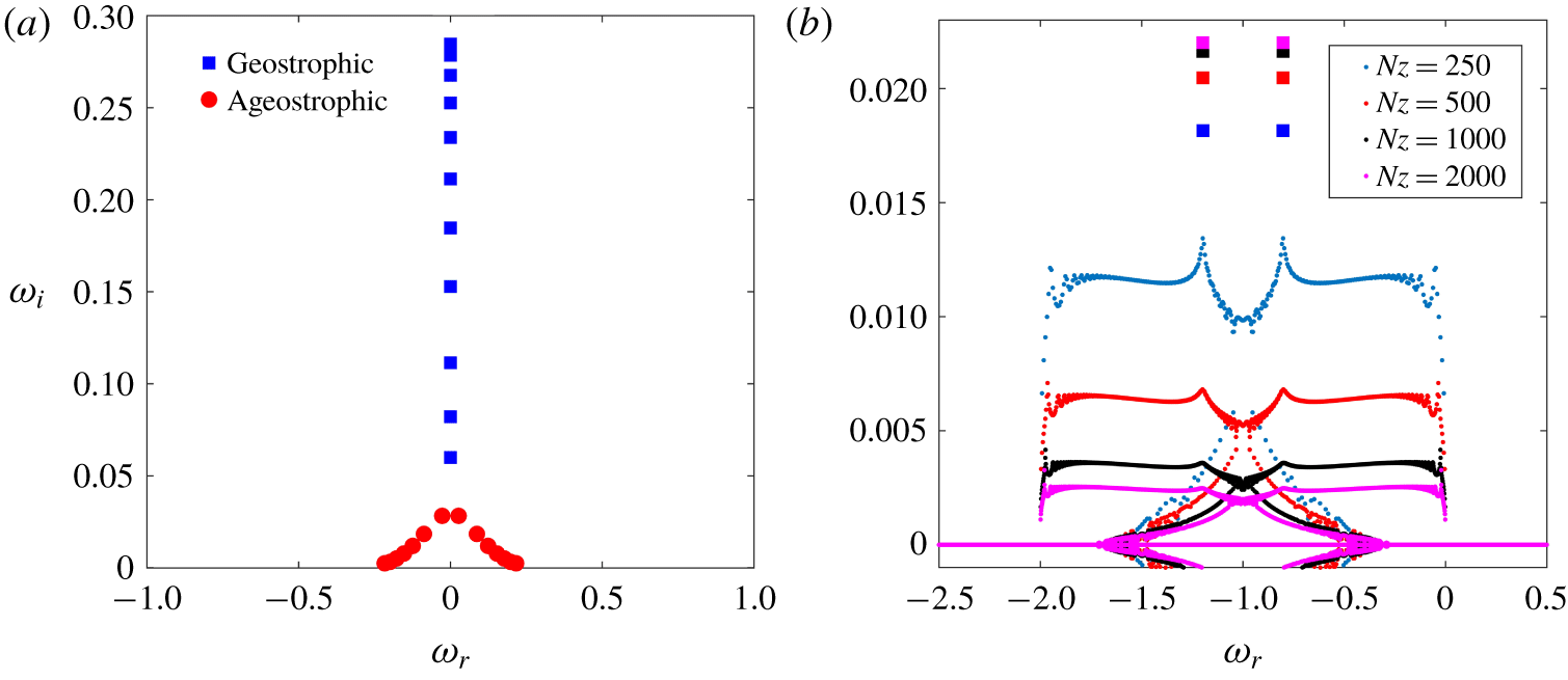
(a) Most unstable eigenvalues rescaled by  $\unicode[STIX]{x1D6FC}$ for geostrophic (blue squares) and ageostrophic (red circles) modes for
 $Ri=0.5$,
 $\unicode[STIX]{x1D6FF}=0.1$,
 $\unicode[STIX]{x1D6FD}=0$ obtained by varying values of
 $\unicode[STIX]{x1D6FC}$. The region with just one unstable eigenmode corresponds to the geostrophic modes, whereas the two ageostrophic modes with same
 $\unicode[STIX]{x1D714}_{i}$ but different
 $\unicode[STIX]{x1D714}_{r}$ emerge at larger
 $\unicode[STIX]{x1D6FC}$. (b) Most unstable eigenvalues and the spurious modes for
 $Ri=0.92$,
 $\unicode[STIX]{x1D6FF}=0.1$,
 $\unicode[STIX]{x1D6FC}=2$,
 $\unicode[STIX]{x1D6FD}=0$ calculated using a different number of vertical discretization points
 $N_{z}$.

For parameter values corresponding to the ageostrophic modes, there are two modes that have the most unstable growth rates, with  $\unicode[STIX]{x1D714}_{r}$ symmetrically distributed about
 $-\unicode[STIX]{x1D6FC}/2$. These modes result from the two critical layers discussed in Nakamura (Reference Nakamura1988) in the ageostrophic regime, and are also found in the eigenspectrum for large
 $\unicode[STIX]{x1D6FC}$ by Heifetz & Farrell (Reference Heifetz and Farrell2007). Analogously, Nakamura (Reference Nakamura1988) finds one critical layer in the geostrophic regime, corresponding to a singular unstable mode shown in figure 1(a). The most unstable modes collapse onto a curve when they are rescaled by
 $\unicode[STIX]{x1D6FC}$, such that
 $(\unicode[STIX]{x1D714}_{r}-\unicode[STIX]{x1D6FC}/2)/\unicode[STIX]{x1D6FC}+\text{i}\unicode[STIX]{x1D714}_{i}/\unicode[STIX]{x1D6FC}$, which is shown in figure 2(a) over a range of
 $\unicode[STIX]{x1D6FC}$ values for
 $Ri=0.5$,
 $\unicode[STIX]{x1D6FF}=0.1$,
 $\unicode[STIX]{x1D6FD}=0$. The structure of the rescaled modes resembles the steering level analysis in Nakamura (Reference Nakamura1988) with one steering level (singular unstable mode) for the geostrophic modes, and two steering levels (two unstable modes) for the ageostrophic modes.
The selection criteria are explained in the following subsections using asymptotic expansions for both the inertial gravity waves and the critical layer modes using dispersion relations. The singular behaviour of critical layers will translate into spurious eigenvalues and eigenvectors with strong oscillations in the vertical direction. The idea in the following is to identify these spurious modes by finding a range of wave frequencies  $\unicode[STIX]{x1D714}$ that represent them in terms of the vertical wavenumber
 $\unicode[STIX]{x1D6FE}$, whose range depends on the number of the vertical discretization points of the domain.
2.4 Inertia–gravity waves
Transient growth arises from the non-normality between eigenvectors. Normal modes that do not project onto the initial optimal perturbation may therefore be discarded prior to computing the optimization procedure for transient growth. In particular, modes with a large wavenumber in the vertical direction are likely to be poorly resolved by the present numerical approach and it is of advantage to identify and remove these modes from the subspace considered for the transient growth analysis.
Inertia–gravity waves, also known as Poincaré waves, are normal by nature and can be recovered from Stone’s equation. Starting with the dimensional form of (2.12)
 $$\begin{eqnarray}\displaystyle & & \displaystyle (\unicode[STIX]{x1D719}^{2}-f^{2})\frac{\text{d}^{2}w}{\text{d}z^{2}}-2\left(\frac{f^{2}\unicode[STIX]{x1D6FC}(\text{d}U/\text{d}z)}{\unicode[STIX]{x1D719}}-\text{i}f\unicode[STIX]{x1D6FD}\frac{\text{d}U}{\text{d}z}\right)\frac{\text{d}w}{\text{d}z}\nonumber\\ \displaystyle & & \displaystyle \quad +\left(-\unicode[STIX]{x1D719}^{2}k^{2}+N^{2}k^{2}-\frac{2\text{i}\unicode[STIX]{x1D6FC}\unicode[STIX]{x1D6FD}(\text{d}U/\text{d}z)^{2}}{\unicode[STIX]{x1D719}}\right)w=0,\end{eqnarray}$$
we seek shear-independent solutions of (2.13) in the near quasi-geostrophic limit (i.e.  $\text{d}U/\text{d}z=\unicode[STIX]{x1D6FF}=0$) and the non-dimensional form of (2.13) reduces to the vertical velocity equation
 $$\begin{eqnarray}(1-(\unicode[STIX]{x1D714}+\unicode[STIX]{x1D6FC}U)^{2})\frac{\text{d}^{2}w}{\text{d}z^{2}}-Ri(\unicode[STIX]{x1D6FC}^{2}+\unicode[STIX]{x1D6FD}^{2})w=0,\end{eqnarray}$$
which is a modified version of the Poincaré wave equation from Heifetz & Farrell (Reference Heifetz and Farrell2003), with a Doppler shift of the eigenvalue frequencies by  $-\unicode[STIX]{x1D6FC}U$. These modes correspond to large oscillations in the vicinity of the critical layers associated with
 $\unicode[STIX]{x1D719}=\unicode[STIX]{x1D714}+\unicode[STIX]{x1D6FC}U=[-1,1]$. The dispersion relation is recovered by setting
 $\text{d}/\text{d}z=\text{i}\unicode[STIX]{x1D6FE}$ and
 $\text{d}^{2}/\text{d}z^{2}=-\unicode[STIX]{x1D6FE}^{2}$ and
 $$\begin{eqnarray}\unicode[STIX]{x1D714}=-\unicode[STIX]{x1D6FC}U\pm \sqrt{1+{\displaystyle \frac{Ri(\unicode[STIX]{x1D6FC}^{2}+\unicode[STIX]{x1D6FD}^{2})}{\unicode[STIX]{x1D6FE}^{2}}}},\end{eqnarray}$$
where  $\unicode[STIX]{x1D6FE}$ is the vertical wavenumber for the short-wavelength oscillations in the vicinity of the critical layers, which depends on the vertical discretization
 $N_{z}$. The modes with this dispersion relation (2.15) are shown in black in figure 1 within the dash-dotted boxes.
2.5 Critical layers
The above dispersion relation allows for discarding of the Poincaré modes located along the real axis but there remain complex conjugate eigenvalues in the vicinity of the Doppler-shifted frequency, shown in red in figure 1. These modes were highlighted by Nakamura (Reference Nakamura1988), damped using viscosity in Heifetz & Farrell (Reference Heifetz and Farrell2003) and are solutions of (2.12) in the near quasi-geostrophic limit. Following Nakamura’s approach (Reference Nakamura1988),  $c=\unicode[STIX]{x1D714}/\unicode[STIX]{x1D6FC}$ is the wave speed and
 $\unicode[STIX]{x1D719}^{2}=(\unicode[STIX]{x1D6FC}U+\unicode[STIX]{x1D714})^{2}=\unicode[STIX]{x1D6FC}^{2}(U+c)^{2}$. Equation (2.13) is non-dimensionalized in the neighbourhood of the critical altitude where
 $U+c=U_{z}H(z-z_{c})$:
 $$\begin{eqnarray}\displaystyle & & \displaystyle (Ro^{2}\unicode[STIX]{x1D6FC}^{2}(z-z_{c})^{2}-1)\frac{\text{d}^{2}w}{\text{d}z^{2}}-2\left(\frac{1}{z-z_{c}}+2\text{i}Ro\,\unicode[STIX]{x1D6FD}\right)\frac{\text{d}w}{\text{d}z}\nonumber\\ \displaystyle & & \displaystyle \quad -\left(\unicode[STIX]{x1D6FC}^{2}k^{2}Ro^{2}\,\unicode[STIX]{x1D6FF}^{2}(z-z_{c})^{2}+k^{2}-\frac{2\text{i}Ro\,\unicode[STIX]{x1D6FD}}{z-z_{c}}\right)w=0.\end{eqnarray}$$
In this limit, the dependence on  $O(Ro^{2})\sim O(z-z_{c})^{2}$ which drops as we seek for solutions
 $z\rightarrow z_{c}$. In the dimensional form, after dividing through by
 $-f^{2}$, equation (2.13) becomes
 $$\begin{eqnarray}\frac{\text{d}^{2}w}{\text{d}z^{2}}+2\left(\frac{\text{d}U/\text{d}z}{U+c}-\frac{\text{i}\unicode[STIX]{x1D6FD}(\text{d}U/\text{d}z)}{f}\right)\frac{\text{d}w}{\text{d}z}+\left(-\frac{N^{2}k^{2}}{f^{2}}-\frac{2\text{i}\unicode[STIX]{x1D6FD}(\text{d}U/\text{d}z)^{2}}{f(U+c)}\right)w=0\end{eqnarray}$$
which in non-dimensional form becomes
 $$\begin{eqnarray}\frac{\text{d}^{2}w}{\text{d}z^{2}}-2\left(\frac{\unicode[STIX]{x1D6FC}}{\unicode[STIX]{x1D714}+\unicode[STIX]{x1D6FC}U}-\text{i}\unicode[STIX]{x1D6FD}\right)\frac{\text{d}w}{\text{d}z}-\left(k^{2}Ri+\frac{2\text{i}\unicode[STIX]{x1D6FC}\unicode[STIX]{x1D6FD}}{\unicode[STIX]{x1D714}+\unicode[STIX]{x1D6FC}U}\right)w=0.\end{eqnarray}$$
The resulting dispersion relation of the Taylor–Goldstein-type equation (2.18) is found to be the same as the Eady (Reference Eady1949) problem (i.e. the near quasi-geostrophic approximation of (2.6) from Nakamura (Reference Nakamura1988)). Thus, we derive our selection criteria by considering the solution of (2.18) where again,  $\text{d}/\text{d}z=\text{i}\unicode[STIX]{x1D6FE}$ and
 $\text{d}^{2}/\text{d}z^{2}=-\unicode[STIX]{x1D6FE}^{2}$. This is equivalent to solving the dispersion relation
 $$\begin{eqnarray}\displaystyle \unicode[STIX]{x1D714} & = & \displaystyle -\frac{\unicode[STIX]{x1D6FE}^{2}\unicode[STIX]{x1D6FC}U+2\text{i}\unicode[STIX]{x1D6FC}\unicode[STIX]{x1D6FE}+2\unicode[STIX]{x1D6FC}\unicode[STIX]{x1D6FD}\unicode[STIX]{x1D6FE}U+k^{2}Ri\,\unicode[STIX]{x1D6FC}U+2\text{i}\unicode[STIX]{x1D6FC}\unicode[STIX]{x1D6FD}}{\unicode[STIX]{x1D6FE}^{2}+2\unicode[STIX]{x1D6FD}\unicode[STIX]{x1D6FE}+k^{2}Ri}\nonumber\\ \displaystyle & = & \displaystyle -\unicode[STIX]{x1D6FC}U-\text{i}\frac{2\unicode[STIX]{x1D6FC}(\unicode[STIX]{x1D6FE}+\unicode[STIX]{x1D6FD})}{\unicode[STIX]{x1D6FE}^{2}+2\unicode[STIX]{x1D6FD}\unicode[STIX]{x1D6FE}+k^{2}Ri}.\end{eqnarray}$$
The eigenmodes that are solutions to (2.18) are shown in figure 1(a,b) with red circles, and the range for their real and imaginary parts can be obtained from the dispersion relation (2.19) shown by the dashed red boxes. The range of  $\unicode[STIX]{x1D714}_{r}$ of these spurious modes is always
 $[-\unicode[STIX]{x1D6FC},0]$ (corresponding to
 $U=z$ and
 $z\in [0,1]$), as has been previously noted by Heifetz & Farrell (Reference Heifetz and Farrell2003), because these modes are associated with the critical layers arising from the singularity
 $\unicode[STIX]{x1D714}+\unicode[STIX]{x1D6FC}U=0$ in (2.12). Hence, these modes are spurious, resulting from the numerical discretization of strong oscillations in the vertical direction near critical layers.
The range of  $\unicode[STIX]{x1D714}_{i}$ in (2.19) is a function of
 $\unicode[STIX]{x1D6FE}$, which depends on the number of vertical discretization points
 $N_{z}$ (
 $\unicode[STIX]{x1D6FE}\geqslant \unicode[STIX]{x03C0}N_{z}$ because these oscillations have wavelengths smaller than
 $\unicode[STIX]{x0394}z$). It is worth noting that the growth rates of the spurious modes increase linearly with increasing mesh sizes
 $\unicode[STIX]{x0394}z$. While we cannot compute the exact values of
 $\unicode[STIX]{x1D714}_{i}$ for each of the spurious modes from (2.19) because we do not a priori know the vertical wavenumber
 $\unicode[STIX]{x1D6FE}$ of each oscillation at each critical layer, we can obtain a range of growth rates for these spurious modes that guides our selection of the physical modes, and allows us to draw the dashed red boxes in figure 1. As we increase
 $N_{z}$, the number of discretization points in the vertical, the growth rates
 $\unicode[STIX]{x1D714}_{i}$ of these spurious modes are dampened but do not converge, unlike those of the physical modes (indicated in green in figure 1) that converge with finer discretizations. The decrease in the growth rates of these unphysical modes is consistent with the dispersion relation (2.19), in which the imaginary part decreases with increasing
 $\unicode[STIX]{x1D6FE}$ (or finer mesh discretization due to larger
 $N_{z}$). An example to illustrate this phenomenon is shown in figure 2(b) for a test case with
 $Ri=0.92$,
 $\unicode[STIX]{x1D6FF}=0.1$,
 $\unicode[STIX]{x1D6FC}=2$,
 $\unicode[STIX]{x1D6FD}=0$. For these spurious modes,
 $\unicode[STIX]{x1D714}_{i}\rightarrow 0$ as
 $N_{z}\rightarrow \infty$, so their growth rates (and their large contribution to transient growth) can be eliminated with sufficiently high discretization (Molemaker et al. Reference Molemaker, McWilliams and Yavneh2005), but the computational time for the direct method that solves for all eigenvalues increase with the cubic power of the order of the matrix (
 $3N_{z}$ for our reduced system (2.7)). However, utilizing the dispersion relation (2.19), we can identify and eliminate the spurious modes at substantially coarser grid resolution without sacrificing the accuracy of the solution.
The unphysical modes, such as the ones that we find, are also known to occur when the number of independent variables in the incompressible Navier–Stokes equations is reduced via algebraic constraints (Manning, Bamieh & Carlson Reference Manning, Bamieh and Carlson2007), as is the case in this paper where we obtain the reduced system (2.8). These modes arise from the numerical approximations, in particular in the vicinity of critical layers, and do not converge as the mesh is refined (Walters & Carey Reference Walters and Carey1983). They have previously been found in many hydrodynamic stability problems, including the numerical solutions of the Orr–Sommerfeld equations for viscid shear flows (Gary & Helgason Reference Gary and Helgason1970; Orszag Reference Orszag1971; Gardner, Trogdon & Douglass Reference Gardner, Trogdon and Douglass1989).
As a result, the only modes considered for the transient growth analysis are depicted in blue in figure 1 together with the unstable mode(s) in green. We show in the following that these modes represent an appropriate subspace for inviscid transient growth calculations. The selected spectra avoid spurious eigenvalues and carefully select resolved eigenvalues in a systematic manner.
3 Transient growth
The system of equations that, when linearized, forms the eigenvalue problem (2.8) and can be generally expressed as an initial value problem, which in the matrix form writes
 $$\begin{eqnarray}\frac{\unicode[STIX]{x2202}\boldsymbol{q}}{\unicode[STIX]{x2202}t}=\unicode[STIX]{x1D645}^{-1}\unicode[STIX]{x1D647}\boldsymbol{q}=\unicode[STIX]{x1D647}_{1}\boldsymbol{q}.\end{eqnarray}$$
Its solution is given by the matrix exponential
 $$\begin{eqnarray}\boldsymbol{q}=\text{e}^{L_{1}t}\boldsymbol{q}_{0}.\end{eqnarray}$$
In the remaining, we seek to maximize the energy gain  $G(T)$ defined by
 $$\begin{eqnarray}G(T)=\underset{E_{0}\neq 0}{\text{max}}\left(\frac{E(T)}{E_{0}}\right)=\underset{\boldsymbol{q}_{0}\neq 0}{\text{max}}\left(\frac{\Vert \boldsymbol{q}(T)\Vert _{E}}{\Vert \boldsymbol{q}_{0}\Vert _{E}}\right)\end{eqnarray}$$
for a given time of optimization  $T$ over all non-zero initial conditions. The norm
 $E(t)$ is the integral of the energy at time
 $t$ and
 $E_{0}$ is the energy of the initial condition
 $\boldsymbol{q}_{0}$, given by the scalar product
 $\Vert \boldsymbol{q}\Vert _{E}=\boldsymbol{q}^{H}M\boldsymbol{q}$. In terms of dimensional variables,
 $\hat{u} ,\hat{v},{\hat{w}},\hat{b}$, it is defined over the computational domain
 $V$ such that
 $$\begin{eqnarray}\hat{E}=\Vert \hat{\boldsymbol{q}}\Vert _{E}=\frac{1}{2}\iiint _{V}\left(\hat{u} ^{2}+\hat{v}^{2}+{\hat{w}}^{2}+\frac{\hat{b}^{2}}{N^{2}}\right)\,\text{d}V,\end{eqnarray}$$
and is the sum of kinetic and available potential energies (Lorenz Reference Lorenz1955; Passaggia, Scotti & White Reference Passaggia, Scotti and White2017; Scotti & Passaggia Reference Scotti and Passaggia2019). The non-dimensionalized energy norm is
 $$\begin{eqnarray}E=\frac{1}{2}\iiint _{V}(\tilde{u} ^{2}+\tilde{v}^{2}+\unicode[STIX]{x1D6FF}^{2}\tilde{w}^{2}+Ri\,\tilde{b}^{2})\,\text{d}V\end{eqnarray}$$
and expressing the perturbation velocities  $\tilde{u}$ and
 $\tilde{v}$ in terms of perturbation vertical vorticity
 $\tilde{\unicode[STIX]{x1D702}}=\text{i}\unicode[STIX]{x1D6FC}\tilde{v}-\text{i}\unicode[STIX]{x1D6FD}\tilde{u}$, the non-dimensional energy norm is
 $$\begin{eqnarray}E=\frac{1}{2}\int _{z}\left(\frac{1}{k^{2}}(D^{2}+\unicode[STIX]{x1D6FF}^{2}k^{2})\tilde{w}^{2}+\frac{1}{k^{2}}\tilde{\unicode[STIX]{x1D702}}^{2}+Ri\,\tilde{b}^{2}\right)\,\text{d}z,\end{eqnarray}$$
with the energy norm matrix
 $$\begin{eqnarray}\unicode[STIX]{x1D648}=\left[\begin{array}{@{}ccc@{}}\left.\left({\displaystyle \frac{D^{2}}{k^{2}}}+\unicode[STIX]{x1D6FF}^{2}\right)\right/2 & 0 & 0\\ 0 & 1/(2k^{2}) & 0\\ 0 & 0 & Ri/2\end{array}\right].\end{eqnarray}$$
The matrix  $\unicode[STIX]{x1D648}$ is positive definite and has a Cholesky decomposition such that
 $\unicode[STIX]{x1D648}=F^{H}F$ for some matrix
 $F$ (Schmid & Henningson Reference Schmid and Henningson2012), and the energy norm for some vectors
 $\boldsymbol{q}_{1}$ and
 $\boldsymbol{q}_{2}$ can be converted to the
 $L_{2}$-norm such that
 $$\begin{eqnarray}(\boldsymbol{q}_{1},\boldsymbol{q}_{2})_{E}=\boldsymbol{q}_{2}^{H}M\boldsymbol{q}_{1}=\boldsymbol{q}_{2}^{H}F^{H}F\boldsymbol{q}_{1}=(F\boldsymbol{q}_{1},F\boldsymbol{q}_{2})_{2}.\end{eqnarray}$$
The optimal transient growth can then be expressed as
 $$\begin{eqnarray}G(t)=\Vert \text{e}^{-\text{i}t\unicode[STIX]{x1D6EC}}\Vert _{E}=\Vert F\text{e}^{-\text{i}t\unicode[STIX]{x1D6EC}}F^{-1}\Vert _{2},\end{eqnarray}$$
where  $\unicode[STIX]{x1D726}$ is the diagonal matrix containing the eigenvalues
 $\unicode[STIX]{x1D714}$ obtained by calculating the normal modal growth after discarding the spurious vectors. The singular value decomposition of the matrix
 $F\text{e}^{-\text{i}t\unicode[STIX]{x1D6EC}}F^{-1}$ yields matrices
 $\unicode[STIX]{x1D650}$,
 $\unicode[STIX]{x1D72E}$ and
 $\unicode[STIX]{x1D651}$. The largest singular value corresponds to
 $G(t)$, whereas the initial conditions associated with the maximum amplification at time
 $t$ are found in the first column of matrix
 $\unicode[STIX]{x1D651}$. The resulting perturbation fields
 $\boldsymbol{q}(t)$ are contained in the first column of matrix
 $\unicode[STIX]{x1D650}$.
4 Results
4.1 Normal modal growth
We begin with the validation of our approach and seek to reproduce the theoretical eigenspectrum of Stone (Reference Stone1970, Reference Stone1971) and the numerical solution of Molemaker et al. (Reference Molemaker, McWilliams and Yavneh2005) with respect to our solution strategy considering the coupled velocity–vorticity–buoyancy in system (2.7). We employ the finite difference-type scheme used by Molemaker et al. (Reference Molemaker, McWilliams and Yavneh2005) who studied the coupled velocity–pressure system and we calculate the normal mode growth rates  $\unicode[STIX]{x1D714}_{i}$ for different values of
 $Ri$,
 $\unicode[STIX]{x1D6FC}$ and
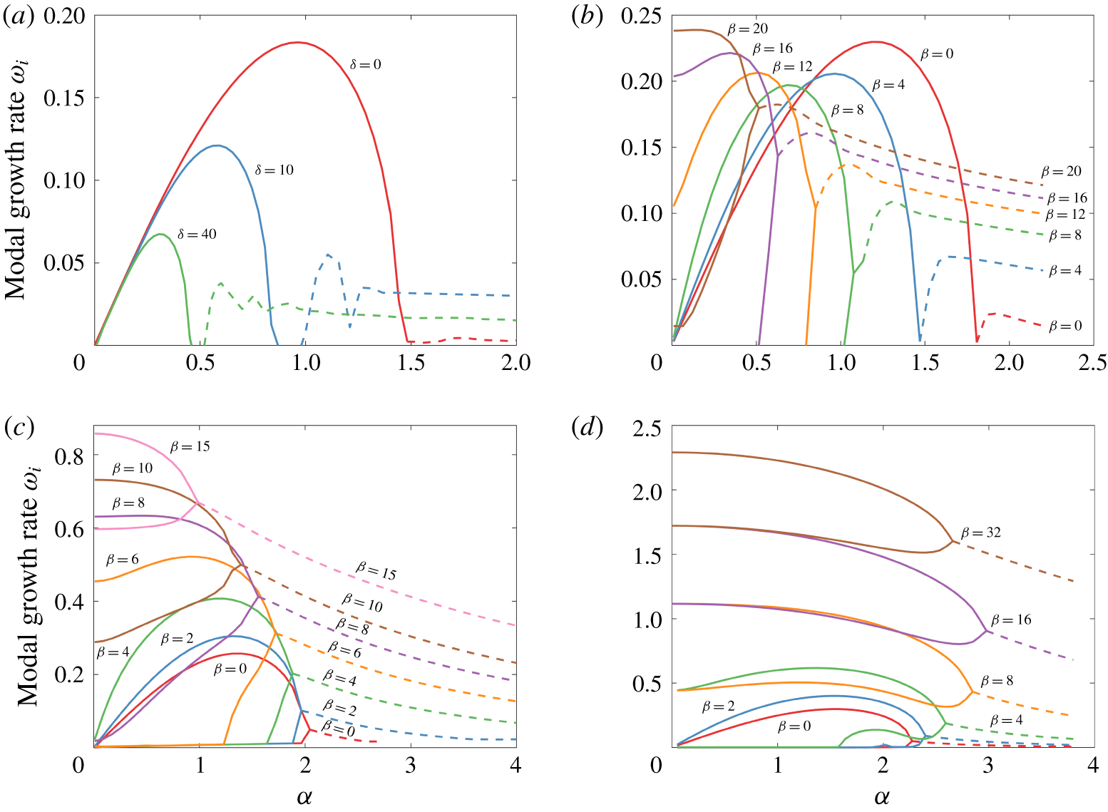
 $\unicode[STIX]{x1D6FD}$. Figure 3(a) shows
 $\unicode[STIX]{x1D714}_{i}$ across
 $\unicode[STIX]{x1D6FC}$ values for
 $Ri=2$ and
 $\unicode[STIX]{x1D6FD}=0$, corresponding to figure 1 in Stone (Reference Stone1970), where it is worth noting that the normal mode growth rates are lower under non-hydrostatic conditions (
 $\unicode[STIX]{x1D6FF}\neq 0$). Figure 3(b–d) shows a sweep over both zonal and meridional wavenumbers under hydrostatic conditions for decreasing values of
 $Ri$, and corresponds to figures 3, 4 and 5 from Stone (Reference Stone1970), respectively. In
 $Ri=0.92$ (figure 3b), we see a transition between the
 $Ri\geqslant 1$ regime where baroclinic instabilities dominate and the
 $Ri<1$ regime where unstable symmetric modes become prominent. At lower
 $\unicode[STIX]{x1D6FD}$ values, the maximum modal growth rate occurs when
 $\unicode[STIX]{x1D6FD}=0$ and decreases with increasing
 $\unicode[STIX]{x1D6FD}$ values, and there are no unstable symmetric modes as there is no growth when the zonal wavenumber
 $\unicode[STIX]{x1D6FC}$ is zero. At higher
 $\unicode[STIX]{x1D6FD}$ values, this growth rate is non-zero for
 $\unicode[STIX]{x1D6FC}=0$, indicating the presence of unstable symmetric modes. At lower
 $Ri$ values (e.g.
 $Ri=0.5$, figure 3c), these instabilities become significant for smaller meridional wavenumber values.
Modal growth rate  $\unicode[STIX]{x1D714}_{i}$ for several values of
 $Ri$,
 $\unicode[STIX]{x1D6FC}$ and
 $\unicode[STIX]{x1D6FD}$. (a)
 $Ri=2$,
 $\unicode[STIX]{x1D6FD}=0$,
 $\unicode[STIX]{x1D6FF}=0$ (hydrostatic) and
 $\unicode[STIX]{x1D6FF}\neq 0$ (non-hydrostatic); (b)
 $Ri=0.92$,
 $\unicode[STIX]{x1D6FF}=0$; (c)
 $Ri=0.5$,
 $\unicode[STIX]{x1D6FF}=0$; (d)
 $Ri=0.1$,
 $\unicode[STIX]{x1D6FF}=0$. In (c,d), both the first and second modes are shown for higher
 $\unicode[STIX]{x1D6FD}$ values. Solid lines indicate geostrophic, and dashed lines indicate ageostrophic instabilities.

For each given  $\unicode[STIX]{x1D6FD}$ value, there are two sets of instabilities: geostrophic for smaller
 $\unicode[STIX]{x1D6FC}$ values (shown in solid lines) and ageostrophic for larger
 $\unicode[STIX]{x1D6FC}$ values (shown in dashed lines). Stone (Reference Stone1970) discussed the possibility of small ageostrophic growth rates even for
 $Ri>1$; while Stone (Reference Stone1970) was unable to verify their existence numerically, these smaller growth rates were later calculated by Molemaker et al. (Reference Molemaker, McWilliams and Yavneh2005), who utilized a high-resolution grid, finer than the number of discretization points used in the present study. We also find the ageostrophic modes for
 $Ri=2$ as shown in figure 3(a), which become more significant in the non-hydrostatic regime.
For  $Ri<1$, there can be more than one unstable eigenmode for certain combinations of
 $\unicode[STIX]{x1D6FC}$ and
 $\unicode[STIX]{x1D6FD}$ values. The growth rates for the first two non-zero unstable eigenmodes are plotted in figure 3(b–d) for
 $Ri=0.92$, 0.5 and 0.1, respectively. These eigenmodes join together at an intermediate
 $\unicode[STIX]{x1D6FC}$ value and continue as an ageostrophic instability for increasing zonal wavenumber values
 $\unicode[STIX]{x1D6FC}$. There are unstable symmetric modes present at these values of
 $Ri$, indicated by the increasing growth rate for
 $\unicode[STIX]{x1D6FC}=0$ and large
 $\unicode[STIX]{x1D6FD}$ values. However, in the case of small
 $\unicode[STIX]{x1D6FD}$, there still exists the dominance of the geostrophic instabilities whose growth rate peaks at
 $\unicode[STIX]{x1D6FD}=0$ and decreases with increasing values of
 $\unicode[STIX]{x1D6FD}$. Figure 3(d) shows the modal growth rates for
 $Ri=0.1$. Both first and second eigenmodes are significantly greater than those at lower
 $Ri$ values for all combinations of
 $\unicode[STIX]{x1D6FC}$ and
 $\unicode[STIX]{x1D6FD}$. This regime is dominated by unstable symmetric modes while their growth rates increase with
 $\unicode[STIX]{x1D6FD}$ for all values of
 $\unicode[STIX]{x1D6FC}$.
4.2 Non-modal growth
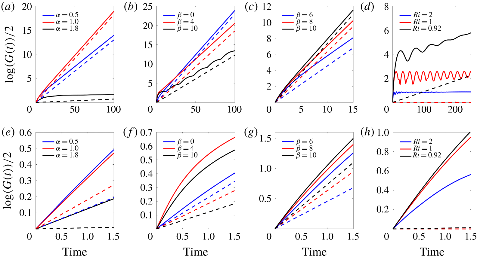
Temporal evolution of energy growth  $\text{log}(G(t))/2$ (solid) and modal growth
 $\unicode[STIX]{x1D714}_{i}t$ (dashed) where the bottom panels are zoomed in on the short-time transient growth. Comparison of geostrophic and ageostrophic modes: (a,e)
 $Ri=2$,
 $\unicode[STIX]{x1D6FD}=0$,
 $\unicode[STIX]{x1D6FC}=0.5,1$ geostrophic,
 $\unicode[STIX]{x1D6FC}=1.8$ ageostrophic; (b,f)
 $Ri=0.92$,
 $\unicode[STIX]{x1D6FC}=1.2$,
 $\unicode[STIX]{x1D6FD}=0,4$ geostrophic,
 $\unicode[STIX]{x1D6FD}=10$ ageostrophic. Symmetric modes: (c,g)
 $Ri=0.5$,
 $\unicode[STIX]{x1D6FC}=0$ and (d,h)
 $\unicode[STIX]{x1D6FC}=0$ and
 $\unicode[STIX]{x1D6FD}=10$ for different
 $Ri$ across the stability boundary predicted by Stone (Reference Stone1970).

A natural approach to validating the optimal transient growth calculation is to consider the long-time asymptotics where for optimization horizons  $T\rightarrow \infty$, the associated transient growth rate
 $\text{log}(G(T))/2T$ should asymptotically converge to the most unstable normal mode growth rate. Hence we study the long-time dynamics for
 $T>100$ and observe the optimal energy gain rate approaching the normal growth rate
 $\unicode[STIX]{x1D714}_{i}$, calculated in § 4.1. Figure 4 shows the optimal energy growth
 $\text{log}(G(t))/2$ (solid lines) and the normal modal growth
 $\unicode[STIX]{x1D714}_{i}t$ (dashed lines) for different combinations of
 $Ri$,
 $\unicode[STIX]{x1D6FC}$ and
 $\unicode[STIX]{x1D6FD}$. For short optimization times, shown in the zoomed-in bottom panels of figure 4, the energy gain
 $G(t)$ can exceed the modal energy gain provided by the modal growth rate quite significantly, indicating the effect of additional non-normal mechanisms, but as
 $t\rightarrow \infty$, the slope of the optimal growth approaches asymptotically that of the modal growth rate
 $\unicode[STIX]{x1D714}_{i}$.
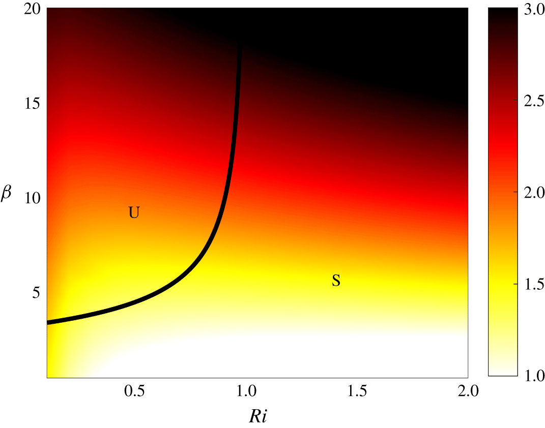
Transient growth rate  $\log G(T=0.5)/2$ for unstable symmetric modes (
 $\unicode[STIX]{x1D6FC}=0$) as a function of
 $Ri$ and
 $\unicode[STIX]{x1D6FD}$. The black curve is a theoretical boundary from Stone (Reference Stone1971); no modal growth is predicted for values of
 $Ri$ and
 $\unicode[STIX]{x1D6FD}$ to the right of the line in the region denoted with ‘S’, and non-zero modal growth is found in the region ‘U’.

We first compare geostrophic and ageostrophic instabilities of pure baroclinic instabilities ( $\unicode[STIX]{x1D6FD}=0$) across
 $\unicode[STIX]{x1D6FC}$ at
 $Ri=2$ in figure 4(a,e) and of mixed modes across
 $\unicode[STIX]{x1D6FD}$ values with
 $\unicode[STIX]{x1D6FC}=1.2$ at
 $Ri=0.92$ in figure 4(b,f). Mixed modes refer to the three-dimensional instabilities where
 $\unicode[STIX]{x1D6FC}\neq 0$ and
 $\unicode[STIX]{x1D6FD}\neq 0$. The growth rates of the ageostrophic instabilities are much more amplified by the transient dynamics than those of the geostrophic modes. At
 $Ri=2$ (figure 4e), the modal growth rate for the ageostrophic mode (
 $\unicode[STIX]{x1D6FC}=1.8$) is 18–25 times smaller than the rates of geostrophic modes (
 $\unicode[STIX]{x1D6FC}=0.5,1$), but its short-time optimal energy growth is only one third of that of the geostrophic modes. For the mixed modes at
 $Ri=0.92$ (figure 4f), the ageostrophic mode (
 $\unicode[STIX]{x1D6FD}=10$) has optimal energy gain comparable to that of the mixed geostrophic mode (
 $\unicode[STIX]{x1D6FD}=4$) and greater than that of the pure geostrophic mode (
 $\unicode[STIX]{x1D6FD}=0$) at short time, despite having half the modal growth rate.
The temporal evolution of the energy growth for the unstable symmetric modes ( $\unicode[STIX]{x1D6FC}=0$) are shown in figure 4(c,g) at
 $Ri=0.5$. The highest rate of the energy growth rate amplification by transient dynamics occurs at low
 $\unicode[STIX]{x1D6FD}$ value: short-term optimal energy gains for symmetric modes with increasing
 $\unicode[STIX]{x1D6FD}=[6,8,10]$ are almost equal even though the modal growth rates vary significantly at
 $[0.45,0.63,0.73]$ for each of the
 $\unicode[STIX]{x1D6FD}$ respectively. Figure 4(e,h) shows unstable symmetric modes
 $\unicode[STIX]{x1D6FD}=10$ for different
 $Ri$ across the stability boundary (see figure 5) from Stone (Reference Stone1970). While the linear stability analysis predicts no energy growth at
 $Ri>1$, we observe considerable non-zero transient energy growth at
 $Ri=1,2$ for several inertial periods. Transient growth rates at
 $T=0.5$ for unstable symmetric modes over a range
 $Ri=[0.1,2]$ and
 $\unicode[STIX]{x1D6FD}=[0.1,20]$ are shown in figure 5. This optimization target time is chosen here as it represents half an inertial period
 $f^{-1}$, which is within the range of the time scale for which the submesoscale instabilities occur (compared with the mesoscale instabilities that occur at time scales greater than the inertial period
 $f^{-1}$) (Boccaletti et al. Reference Boccaletti, Ferrari and Fox-Kemper2007). The black curve is a theoretical boundary calculated from equation (4.8) in Stone (Reference Stone1971), which prescribes values of
 $\unicode[STIX]{x1D6FD}$ as a function of
 $Ri$ where modal growth rates decrease down to zero. For values of
 $Ri$ and
 $\unicode[STIX]{x1D6FD}$ to the right of this curve (region marked by ‘S’), modal growth rates for unstable symmetric modes are zero, but as figure 5 shows, transient growth rates can be significant outside of this boundary, even for
 $Ri>1$.
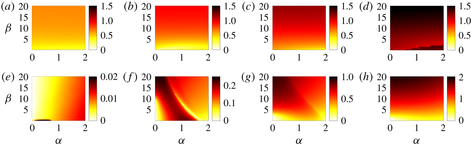
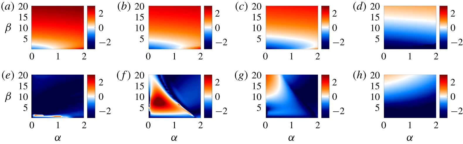
We conduct parameter sweeps over  $\unicode[STIX]{x1D6FC}=[0,2]$ and
 $\unicode[STIX]{x1D6FD}=[0.3,20]$ for transient (at
 $T=0.5$) and normal growth rates shown in figure 6(a–h), respectively. The growth rates are computed at
 $Ri=2$ (a,e), 0.92 (b,f), 0.5 (c,g) and 0.1 (d,h) to compare different regimes. As
 $Ri$ decreases, both transient growth and normal growth rates increase, but the amplification of the normal growth rate by the transient dynamics decreases. In general, we find that transient growth rates at a given
 $Ri$ are mostly independent of
 $\unicode[STIX]{x1D6FC}$ and increase with
 $\unicode[STIX]{x1D6FD}$, while the normal growth rates are more complex functions of both
 $\unicode[STIX]{x1D6FC}$ and
 $\unicode[STIX]{x1D6FD}$. Transient growth especially exceeds modal growth at high Richardson numbers for modes with moderate to large meridional wavenumbers
 $\unicode[STIX]{x1D6FC}$, including the three-dimensional modes where
 $\unicode[STIX]{x1D6FD}\neq 0$. In contrast, pure geostrophic modes (small
 $\unicode[STIX]{x1D6FC}$,
 $\unicode[STIX]{x1D6FD}=0$) do not seem to gain as much from the transient growth. The transient growth rates of unstable symmetric modes are much larger (up to several orders of magnitude) than the modal growth rates at higher
 $Ri$ and/or at lower
 $\unicode[STIX]{x1D6FD}$. When
 $Ri$ is small (figure 6c,d,g,h), unstable symmetric modes have substantial modal growth rates, and the transient growth rates are only larger by approximately a factor two.
These results are in agreement with the study of Heifetz & Farrell (Reference Heifetz and Farrell2007) who considered a few cases of horizontally isotropic perturbations such as ( $\unicode[STIX]{x1D6FC}=\unicode[STIX]{x1D6FD}=[0.1,1,10]$) at
 $Ri=1$. In the case
 $\unicode[STIX]{x1D6FC}=\unicode[STIX]{x1D6FD}=1$, they report a maximum instantaneous growth rate
 $\text{log}(G)\approx 0.5$ at
 $Ri=1$ which is very close to the value of 0.49 that we report in figure 6(b) at
 $T=0.5$. We find transient growth rates of 0.26 and 2.0 for
 $\unicode[STIX]{x1D6FC}=\unicode[STIX]{x1D6FD}=0.1$ and
 $\unicode[STIX]{x1D6FC}=\unicode[STIX]{x1D6FD}=10$, respectively, which also agree with values in Heifetz & Farrell (Reference Heifetz and Farrell2007) (0.26 and 2.2, respectively). Note that Heifetz & Farrell (Reference Heifetz and Farrell2003, Reference Heifetz and Farrell2007, Reference Heifetz and Farrell2008) report the instantaneous transient growth rates (i.e. at
 $T=0$), whereas we compute optimal growth rates at
 $T=0.5$, which is lower than the instantaneous growth rate.
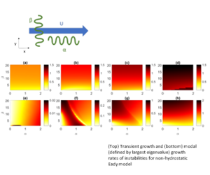
(a,b,c,d) Transient and (e,f,g,h) normal growth rates as functions of  $\unicode[STIX]{x1D6FC}=[0,2]$ and
 $\unicode[STIX]{x1D6FD}=[0.3,20]$. (a,e)
 $Ri=2$, (b,f)
 $Ri=0.92$, (c,g)
 $Ri=0.5$ and (d,h)
 $Ri=0.1$. Transient growth rates
 $\log (G(T))/2T$ are found at
 $T=0.5$.

4.3 Non-hydrostatic effects on transient growth
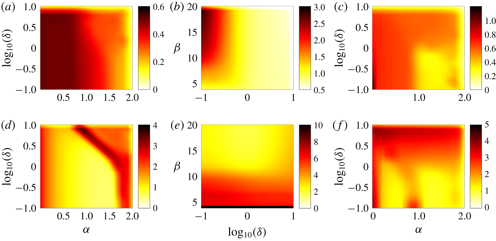
(a,b,c) Transient growth rates  $\text{log}(G(T))/T$ and (d,e,f) log plot of
 $\text{log}(G(T))/\unicode[STIX]{x1D714}_{i}T$ at
 $T=0.5$ as functions of
 $\unicode[STIX]{x1D6FC}=[0,2]$,
 $\unicode[STIX]{x1D6FD}=[0,20]$ and
 $\unicode[STIX]{x1D6FF}=[0.1,10]$ for
 $Ri=0.92$. (a,d) baroclinic instabilities with
 $\unicode[STIX]{x1D6FD}=0$, (b,e) unstable symmetric modes with
 $\unicode[STIX]{x1D6FC}=0$, (c,f) mixed modes with
 $\unicode[STIX]{x1D6FD}=10$. In (e),
 $\unicode[STIX]{x1D6FD}<4$ is truncated as the modal growth rates approach zero, so the amplification by the transient growth approaches infinity.

The non-hydrostatic effects have been previously overlooked, mainly because the coupled system (2.6) in the  $\unicode[STIX]{x1D6FF}\rightarrow 0$ limit allows for reducing the number of variables and efficiently solving the associated eigenvalue and generalized stability problems (cf. Heifetz & Farrell (Reference Heifetz and Farrell2003, Reference Heifetz and Farrell2007, Reference Heifetz and Farrell2008)). In this section, we study the non-hydrostatic effects by varying the parameter
 $\unicode[STIX]{x1D6FF}=(H/L)/Ro=fH/u_{0}$, which for a fixed
 $Ri$ is equivalent to varying the aspect ratio
 $H/L$. In an ocean mixed layer of
 $O(100~\text{m})$ at mid-latitudes
 $\unicode[STIX]{x1D6FF}$ values can reach up to 0.1, which corresponds to the ocean values reported in Boccaletti et al. (Reference Boccaletti, Ferrari and Fox-Kemper2007) off the coast of California and in the Gulf Stream (Callies et al. Reference Callies, Ferrari, Klymak and Gula2015).
However, the dynamics at  $\unicode[STIX]{x1D6FF}\sim 1$ or greater may be significant, for instance in the eye wall region in the case of tornadoes (Nolan et al. Reference Nolan, Dahl, Bryan and Rotunno2017) and hurricanes (Worsnop et al. Reference Worsnop, Lundquist, Bryan, Damiani and Musial2017). The average aspect ratios of the hurricane boundary layer rolls reported in observations for the Atlantic hurricanes (Foster Reference Foster2013) and Pacific typhoons (Ellis & Businger Reference Ellis and Businger2010) fall around
 $H/L\simeq 0.5$ but can exceed unity, and these rolls can have significant impact on the vertical momentum flux in hurricanes (Morrison et al. Reference Morrison, Businger, Marks, Dodge and Businger2005).
Using asymptotic analysis, Stone (Reference Stone1971) showed that for baroclinic instabilities, modal growth rates are reduced as  $\unicode[STIX]{x1D6FF}$ increases (see figure 3a). We, therefore, analysed the effect of non-zero values of
 $\unicode[STIX]{x1D6FF}$ on the transient growth dynamics, which generalizes the findings of Heifetz & Farrell (Reference Heifetz and Farrell2003, Reference Heifetz and Farrell2007, Reference Heifetz and Farrell2008). While for the geophysical applications,
 $\unicode[STIX]{x1D6FF}\simeq 1$ may be the upper bound, we generalize our findings for
 $\unicode[STIX]{x1D6FF}=[0,10]$ to fully investigate the non-hydrostatic effects. Figure 7(a–c) shows how transient growth rates
 $\text{log}(G(T))/2$ found at
 $T=0.5$ are affected by
 $\unicode[STIX]{x1D6FF}$, and (d–f) show the amplification of modal growth rates by optimal linear dynamics for selected parameter spaces at
 $Ri=0.92$. Figure 7(a,d) focuses on baroclinic instabilities with
 $\unicode[STIX]{x1D6FC}=[0,2]$, figure 7(b,e) on unstable symmetric modes with
 $\unicode[STIX]{x1D6FD}=[0,20]$ and figure 7(c,f) explores mixed modes with
 $\unicode[STIX]{x1D6FD}=10$ and
 $\unicode[STIX]{x1D6FC}=[0,2]$. The transient growth rates are mostly independent of
 $\unicode[STIX]{x1D6FF}$ and are larger at lower
 $\unicode[STIX]{x1D6FC}$ values. The structure of
 $\text{log}(G(T))/2\unicode[STIX]{x1D714}_{i}$ is influenced by the dependence of modal growth rates on
 $\unicode[STIX]{x1D6FC}$ and
 $\unicode[STIX]{x1D6FF}$. Transient growth rates do not change significantly with
 $\unicode[STIX]{x1D6FD}$ or
 $\unicode[STIX]{x1D6FF}$ values, except in the small
 $\unicode[STIX]{x1D6FF}$ regime in which
 $\text{log}(G(T))/2$ increases with
 $\unicode[STIX]{x1D6FD}$. At low
 $\unicode[STIX]{x1D6FD}$ values for all
 $\unicode[STIX]{x1D6FF}$,
 $\unicode[STIX]{x1D714}_{i}\simeq 0$, whereas transient growth rates are non-zero. The amplification of modal growth rates by optimal perturbation decreases with
 $\unicode[STIX]{x1D6FD}$ with less significant dependence on
 $\unicode[STIX]{x1D6FF}$.
4.4 Energy budget of transient and modal growth
We further investigate the effect of transient growth on the energy transfers with an emphasis on the partition between shear production and buoyancy fluxes. One of the important aspects of transient growth is to provide alternative mechanisms for vertical transport or the vertical restratification. In particular we quantify the ratio of horizontal buoyancy flux to the production of kinetic energy. While the first redistributes potential energy in the horizontal direction, the second relates to the amount of vertical transport.
From (3.6), the rate of change of energy in non-dimensional form is
 $$\begin{eqnarray}\frac{\unicode[STIX]{x2202}E}{\unicode[STIX]{x2202}t}=\frac{1}{2}\frac{\unicode[STIX]{x2202}}{\unicode[STIX]{x2202}t}\int _{V}\left(2u\frac{\unicode[STIX]{x2202}u}{\unicode[STIX]{x2202}t}+2v\frac{\unicode[STIX]{x2202}v}{\unicode[STIX]{x2202}t}+2\unicode[STIX]{x1D6FF}^{2}w\frac{\unicode[STIX]{x2202}w}{\unicode[STIX]{x2202}t}+2Ri\,b\frac{\unicode[STIX]{x2202}b}{\unicode[STIX]{x2202}t}\right)\,\text{d}V.\end{eqnarray}$$
Taking  $\unicode[STIX]{x1D701}=\text{e}^{\text{i}(\unicode[STIX]{x1D6FC}x+\unicode[STIX]{x1D6FD}y+\unicode[STIX]{x1D714}t)}$, we have
 $q=\tilde{q}(z)\unicode[STIX]{x1D701}$ and
 $q_{t}=\text{i}\unicode[STIX]{x1D714}\tilde{q}(z)\unicode[STIX]{x1D701}$.
The equation for the rate of change of energy can be re-written as
 $$\begin{eqnarray}\frac{\unicode[STIX]{x2202}E}{\unicode[STIX]{x2202}t}=\text{i}\unicode[STIX]{x1D714}\int _{x}\int _{y}\unicode[STIX]{x1D701}^{2}\int _{z}(\tilde{u} ^{2}+\tilde{v}^{2}+\unicode[STIX]{x1D6FF}^{2}\tilde{w}^{2}+Ri\,\tilde{b}^{2})\,\text{d}z\,\text{d}y\,\text{d}x.\end{eqnarray}$$
Multiplying the non-dimensional linearized governing equations (2.6a–d) by  $\tilde{u}$,
 $\tilde{v}$,
 $\tilde{w}$ and
 $\tilde{b}$ respectively, we get an expression for the energy rate of change
 $$\begin{eqnarray}\frac{\unicode[STIX]{x2202}E}{\unicode[STIX]{x2202}t}=\text{i}\unicode[STIX]{x1D714}\int _{x}\int _{y}\unicode[STIX]{x1D701}^{2}\int _{z}(-\tilde{u} \tilde{w}+\tilde{v}\tilde{b}-\text{i}\unicode[STIX]{x1D6FC}UE)\,\text{d}z\,\text{d}y\,\text{d}x,\end{eqnarray}$$
where the three terms on the right are shear production, meridional buoyancy flux and horizontal energy transport. Here, the terms are non-dimensional and the background shear  $\text{d}U/\text{d}z=1$ in the shear production term
 $-uw\,\text{d}U/\text{d}z$. It should be noted that the last term does not play a role in the energy balance equation and only characterizes the zonal advection of energy. This analysis is somewhat different than the analysis of Stamper & Taylor (Reference Stamper and Taylor2017) where they only characterize the kinetic energy budget. Instead we consider the total energy budget where the vertical buoyancy flux cancels out.
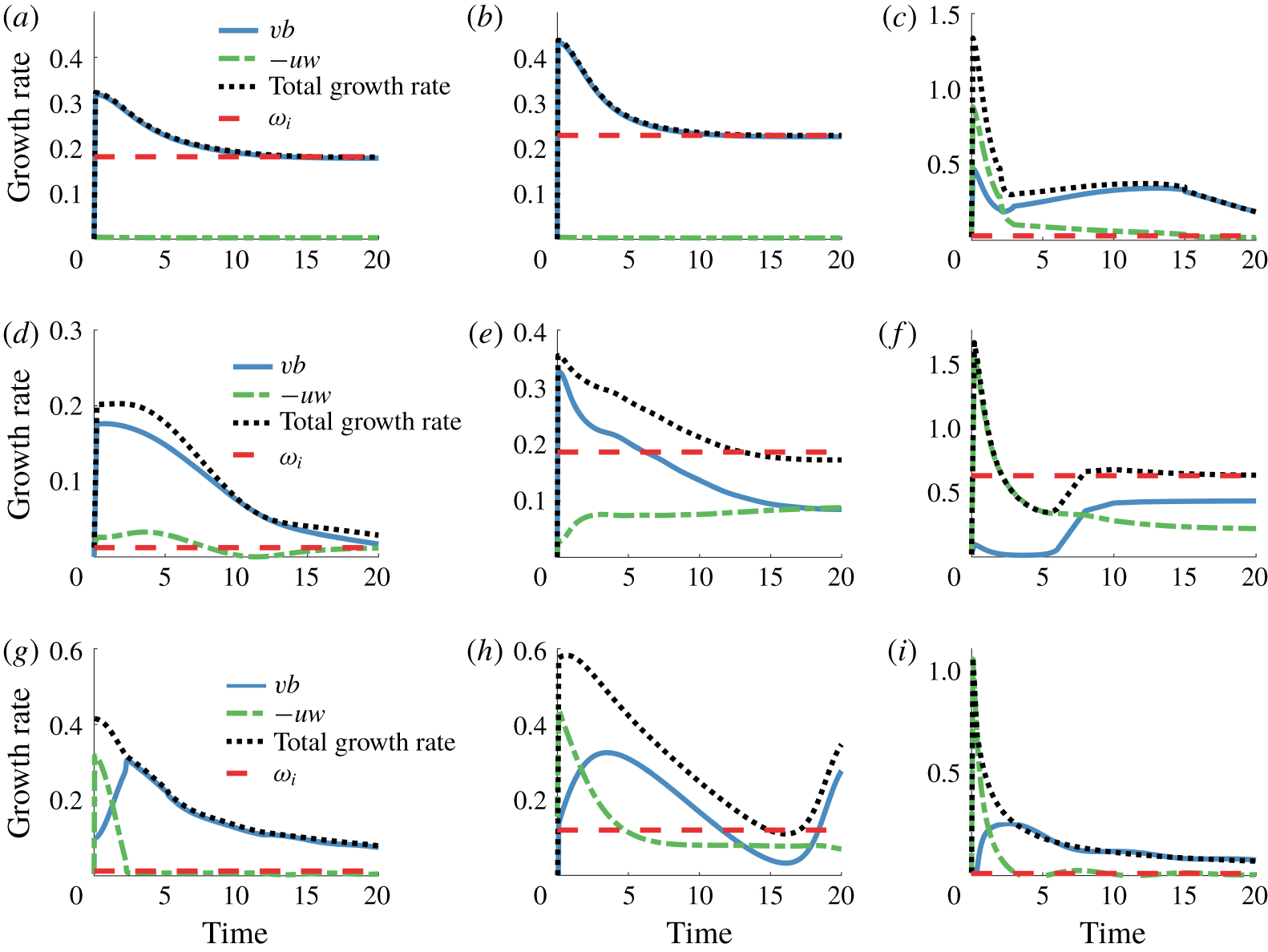
Optimal energy growth rate at optimization time  $t$ (meridional buoyancy flux: blue solid; shear production: green dash-dotted; total: black dotted lines) and modal growth rate
 $\unicode[STIX]{x1D714}_{i}$ (red dashed line). (a,d,g)
 $Ri=2$ (a) geostrophic mode (
 $\unicode[STIX]{x1D6FC}=1$,
 $\unicode[STIX]{x1D6FD}=0$), (d,g) ageostrophic modes (
 $\unicode[STIX]{x1D6FC}=1.8$,
 $\unicode[STIX]{x1D6FD}=0,4$); (b,e,h)
 $Ri=0.92$,
 $\unicode[STIX]{x1D6FC}=1.2$ (b,e) geostrophic modes (
 $\unicode[STIX]{x1D6FD}=0,4$), (h) ageostrophic mode (
 $\unicode[STIX]{x1D6FD}=10$); (c,f,i) symmetric modes (
 $\unicode[STIX]{x1D6FC}=0$) (c)
 $Ri=0.5$,
 $\unicode[STIX]{x1D6FD}=2$, (f)
 $Ri=0.5$,
 $\unicode[STIX]{x1D6FD}=10$, (i)
 $Ri=2$,
 $\unicode[STIX]{x1D6FD}=10$. All values are computed for
 $\unicode[STIX]{x1D6FF}=0.1$.

Figure 8 shows the time series of instantaneous growth rate split between the meridional buoyancy flux and shear production along with the modal growth rate for selected cases presented in figure 4. The left panels show (a) geostrophic ( $[\unicode[STIX]{x1D6FC},\unicode[STIX]{x1D6FD}]=[1,0]$) and (d,g) ageostrophic (
 $[\unicode[STIX]{x1D6FC},\unicode[STIX]{x1D6FD}]=[1.8,0]$,
 $[\unicode[STIX]{x1D6FC},\unicode[STIX]{x1D6FD}]=[1.8,4]$) modes for
 $Ri=2$. The middle panels show (b,e) geostrophic (
 $[\unicode[STIX]{x1D6FC},\unicode[STIX]{x1D6FD}]=[1.2,0]$,
 $[\unicode[STIX]{x1D6FC},\unicode[STIX]{x1D6FD}]=[1.2,4]$) and (h) ageostrophic (
 $[\unicode[STIX]{x1D6FC},\unicode[STIX]{x1D6FD}]=[1.2,10]$) modes for
 $Ri=0.92$. The right panels show symmetrically unstable modes (
 $\unicode[STIX]{x1D6FC}=0$) for (c,f)
 $Ri=0.5$ with
 $\unicode[STIX]{x1D6FD}$ values: (c)
 $\unicode[STIX]{x1D6FD}=2$ and (f)
 $\unicode[STIX]{x1D6FD}=10$ and (i)
 $Ri=2,\unicode[STIX]{x1D6FD}=0.$ As
 $t\rightarrow \infty$, the growth rate approaches
 $\unicode[STIX]{x1D714}_{i}$, validating our calculations.
For geostrophic modes at  $Ri>2$ (figure 8a) and
 $Ri<1$ (figure 8b), the meridional buoyancy flux dominates over the shear production, which is close to zero, consistent with results presented in the middle panels of figure 7 in Heifetz & Farrell (Reference Heifetz and Farrell2007) at
 $Ri=1,\unicode[STIX]{x1D6FC}=\unicode[STIX]{x1D6FD}=1$. In contrast, in the case of ageostrophic modes, for which energy growth is much more amplified by the optimal linear dynamics than for geostrophic modes, the proportion of energy gain from shear production becomes greater (figure 8d) or even exceeds the energy gain from meridional buoyancy flux (figure 8g,h). This result is also qualitatively consistent with Heifetz & Farrell (Reference Heifetz and Farrell2007) (cf. their figure 7 bottom panels) for
 $\unicode[STIX]{x1D6FC}=\unicode[STIX]{x1D6FD}=10$. We observe that the increase in the proportion of energy gain from shear production at short time can be obtained through transition from the geostrophic to ageostrophic instability regime by increasing
 $\unicode[STIX]{x1D6FC}$ (compare figures 8a and 8d) or increasing
 $\unicode[STIX]{x1D6FD}$ (compare progression in figure 8d,e and in b,e,h). However, at long time, the energy gain is primarily drawn from the meridional buoyancy flux. Our analysis here shows that there is a strong vertical momentum flux characteristic of ageostrophic modes at short times
 $T<5$, in contrast with geostrophic instabilities for which the dominant meridional buoyancy flux that distributes the lateral buoyancy gradient horizontally. This difference in the energy pathways between geostrophic and ageostrophic modes is important because, as Boccaletti et al. (Reference Boccaletti, Ferrari and Fox-Kemper2007) noted, the ageostrophic instabilities could be significant due their time scales being less than the geostrophic adjustment time scale (
 $O(f^{-1})$).
For unstable symmetric modes, the contribution of shear production to energy gain also increases with increasing  $\unicode[STIX]{x1D6FD}$ value (compare figures 8c and 8f). However, at longer time, the contribution from buoyancy flux becomes equal to or exceeds the shear production (see figure 8c,f,i). Grisouard (Reference Grisouard2018) similarly showed a significant contribution from the energy drawn from the potential energy of the mean flow in two-dimensional numerical simulations of unstable symmetric modes. We will further explore this behaviour in the next section using the optimal initial conditions for the growth in the finite amplitude regime.
Parameter sweep over  $\unicode[STIX]{x1D6FC}=[0,2]$ and
 $\unicode[STIX]{x1D6FD}=[0.3,20]$ of
 $\log (\unicode[STIX]{x1D6E4}(\unicode[STIX]{x1D6FC},\unicode[STIX]{x1D6FD}))$, where
 $\unicode[STIX]{x1D6E4}$ is the ratio of shear production
 $-\tilde{u} \tilde{w}$ to meridional buoyancy flux
 $\tilde{v}\tilde{b}$ (a,b,c,d) at
 $T=0.5$ where transient growth occurs, (e,f,g,h) for normal growth: (a,e)
 $Ri=2$, (b,f)
 $Ri=0.92$, (c,g)
 $Ri=0.5$ and (d,h)
 $Ri=0.1$.

As shown from the energy norm in (4.3), we only need to consider the ratio of shear production to meridional buoyancy flux to characterize the exchanges in energy. Figure 9 shows the log of the ratio,  $\unicode[STIX]{x1D6E4}$, defined as
 $$\begin{eqnarray}\unicode[STIX]{x1D6E4}=\frac{\displaystyle \int -\tilde{u} \tilde{w}\,\text{d}z}{\displaystyle \int \tilde{v}\tilde{b}\,\text{d}z},\end{eqnarray}$$
for various values of  $Ri$ as functions of
 $\unicode[STIX]{x1D6FC}$ and
 $\unicode[STIX]{x1D6FD}$. Figure 9(a–d) shows
 $\log (\unicode[STIX]{x1D6E4})$ calculated at short times of optimization
 $T=0.5$, whereas figure 9(e–h) shows log(
 $\unicode[STIX]{x1D6E4}$) for normal growth. The patterns of ratio of shear production stress to buoyancy flux are strikingly different between normal mode and transient growth dynamics. Figure 9(g) matches figure 2(a) in Stamper & Taylor (Reference Stamper and Taylor2017). For transient growth, this ratio is higher at larger
 $Ri$; as
 $Ri$ decreases, the region where the meridional buoyancy flux is greater than shear production grows. This progression can be explained by the transition from geostrophic to ageostrophic modes occurring at larger
 $\unicode[STIX]{x1D6FC}$ as
 $Ri$ decreases (see figure 3).
At optimization time  $T=0.5$, for
 $Ri>1$ (figure 9a), the shear production is greater than the buoyancy flux for almost all values of
 $\unicode[STIX]{x1D6FC}$ and
 $\unicode[STIX]{x1D6FD}$, except in a small region at low
 $\unicode[STIX]{x1D6FC}$ and
 $\unicode[STIX]{x1D6FD}$ values, where the two energy fluxes are roughly equal or the meridional buoyancy flux is dominant. This corresponds to the region of higher normal mode growth rate in figure 9(a) due to geostrophic baroclinic instabilities. At intermediate
 $Ri$ values (
 $0.25<Ri<1$), the buoyancy flux is dominant where both
 $\unicode[STIX]{x1D6FC}$ and
 $\unicode[STIX]{x1D6FD}$ are small (figure 9b,c). Shear production becomes more dominant as unstable symmetric modes become stronger (large
 $\unicode[STIX]{x1D6FD}$ values) and/or as ageostrophic instabilities emerge (large
 $\unicode[STIX]{x1D6FC}$ values). At low
 $Ri$ values (
 $Ri\leqslant 0.25$), the region where the meridional buoyancy flux is dominant is larger than at higher
 $Ri$ values (figure 9d). Vertical stratification becomes weaker as
 $Ri$ decreases, while the horizontal buoyancy gradient that could drive the meridional buoyancy flux increases. Numerical simulations by Arobone & Sarkar (Reference Arobone and Sarkar2015) similarly showed that near-symmetric unstable modes generate flows that do not align with isopycnals and draw energy from the available potential energy reservoir of the background flow for several initial inertial periods. However, as
 $\unicode[STIX]{x1D6FD}$ increases, unstable symmetric modes become more dominant and
 $\unicode[STIX]{x1D6E4}$ becomes greater than 1.
This analysis shows that in the asymptotic limit as  $t\rightarrow \infty$, the meridional transport overwhelms the shear production for a large portion of the
 $[Ri,\unicode[STIX]{x1D6FC},\unicode[STIX]{x1D6FD}]$ parameter space (see figure 9e–h) with the exception of some mixed modes at
 $Ri=0.92$ and small regions of large-
 $\unicode[STIX]{x1D6FD}$ unstable symmetric modes at low
 $Ri$. However, we stress that it is not the case for the linear optimal perturbations, where for symmetric modes with large values of
 $\unicode[STIX]{x1D6FD}$ and ageostrophic modes with large
 $\unicode[STIX]{x1D6FC}$ and/or
 $\unicode[STIX]{x1D6FD}$ values, the shear production is either equally important to or dominates the energetic dynamics.
4.5 Mechanisms of transient growth
In order to investigate the difference in amplification of growth rates by transient growth in geostrophic, ageostrophic and symmetric modes, we study the evolution of the eigenvectors’ profiles associated with the most unstable eigenmodes and optimal initial conditions that lead to optimal growth. As discussed in § 4.4, the shear production is a greater contributor to the energy budget than the meridional buoyancy flux at short times for ageostrophic modes and symmetric modes. For this family of modes, the amplification of modal growth rates by transient dynamics is also greater than for geostrophic modes, for which meridional buoyancy flux is dominant over the shear production. In this section, we explore the mechanisms that are responsible for the differences in transient growth between each family of modes.
Figure 10 shows buoyancy cross-sections of strongly amplified representative unstable modes in (a,d,g), buoyancy cross-sections of initial conditions leading to optimal perturbation at  $T=0.5$ in (b,e,h) and three-dimensional structures of optimal initial conditions for vertical velocity in (c,f,i). All modes shown are for
 $Ri=2$ and
 $\unicode[STIX]{x1D6FF}=0.1$. The geostrophic mode with
 $[\unicode[STIX]{x1D6FC},\unicode[STIX]{x1D6FD}]=[1,0]$ has vortices that are uniform in the meridional direction with
 $z$-dependent vertical velocity perturbations (figure 10c), and the buoyancy profiles for both the most unstable eigenmode and the optimal initial conditions that are aligned with the background shear, indicated by black lines in figures 10(a) and 10(b), respectively. We observe that both modal and optimal transient energy predominantly grow due to the meridional buoyancy flux (i.e. given by
 $vb$) for the geostrophic modes (see figure 8a) and there is not as great of an amplification of growth rates by optimal perturbations (the transient growth rate is only twice the modal growth rate for this test case).
(a,d,g) Zonal–vertical buoyancy cross-sections of most unstable mode (a,d) and meridional–vertical buoyancy cross-section of the first mode (stable) (g), (b,e,h) zonal–vertical (b,e) and meridional–vertical (h) cross-sections of optimal perturbation initial condition for buoyancy, and (c,f,i) three-dimensional structure of optimal perturbation initial condition for vertical velocity. Panels (a–c) are for the geostrophic mode  $[\unicode[STIX]{x1D6FC},\unicode[STIX]{x1D6FD}]=[1,0]$, (d–f) are for the ageostrophic mode
 $[\unicode[STIX]{x1D6FC},\unicode[STIX]{x1D6FD}]=[1.8,0]$, (g–i) are for the symmetric mode
 $[\unicode[STIX]{x1D6FC},\unicode[STIX]{x1D6FD}]=[0,10]$, which does not have any unstable modes. All values are for
 $Ri=2$ and
 $\unicode[STIX]{x1D6FF}=0.1$. Black lines in (a,b,d,e) represent the background zonal velocity
 $U(z)$ and black lines in (g,h) represent the background buoyancy
 $B(y,z)$.

Temporal evolution of the difference between the optimal initial condition and the contribution of the unstable (or first) mode. (a–c) Geostrophic mode  $\unicode[STIX]{x1D6FC}=1$,
 $\unicode[STIX]{x1D6FD}=0$,
 $Ri=2$,
 $\unicode[STIX]{x1D6FF}=0.1$, (d–f) ageostrophic mode
 $\unicode[STIX]{x1D6FC}=1.8$,
 $\unicode[STIX]{x1D6FD}=0$,
 $Ri=2$,
 $\unicode[STIX]{x1D6FF}=0.1$ and (g–i) symmetric mode
 $\unicode[STIX]{x1D6FC}=0$,
 $\unicode[STIX]{x1D6FD}=10$,
 $Ri=2$,
 $\unicode[STIX]{x1D6FF}=0.1$. The arrows at the initial time show the direction of the perturbation travel toward the boundary or critical layer, and the arrows at later time show the reflection types (backward, forward, critical).

Buoyancy cross-sections and vertical velocity structure for ageostrophic mode with  $[\unicode[STIX]{x1D6FC},\unicode[STIX]{x1D6FD}]=[1.8,0]$ are shown in figure 10(d–f). The vertical velocity forms meridionally uniform vortices similar to those of the geostrophic mode, but they are sheared near the vertical boundaries. The buoyancy profiles are significantly different between the most unstable mode and the optimal initial perturbation. Shear production (i.e. given by
 $-uw$) makes a non-zero contribution to the energy growth at short times for the optimal perturbations and the modal growth rates are substantially amplified by the optimal perturbations (the transient growth rate is 13 times greater for this test case).
For a flow with a background thermal wind balance, wave-like instabilities can undergo critical reflection off horizontal surfaces and can lead to the irreversible energy exchange with the background flow (Grisouard & Thomas Reference Grisouard and Thomas2015, Reference Grisouard and Thomas2016). These reflections can be of three types, depending on the wave frequency: (i) backward reflection ( $\unicode[STIX]{x1D714}<1$), (ii) critical reflection (
 $\unicode[STIX]{x1D714}=1$) and (iii) forward reflection (
 $\unicode[STIX]{x1D714}>1$). Here we use wave frequency non-dimensionalized by
 $f$. As noted by Nakamura (Reference Nakamura1988), critical layers can also serve as horizontal surfaces for the reflections of the instabilities in addition to the top and bottom boundaries. In figure 11, the temporal evolution of the remainder between the optimal initial condition and the most unstable mode are shown to determine whether reflections, observed by Grisouard & Thomas (Reference Grisouard and Thomas2015, Reference Grisouard and Thomas2016) occur for these instabilities. This residual perturbation was computed using the expression
 $\tilde{\boldsymbol{q}}(t)-\boldsymbol{q}^{\dagger ,H}\tilde{\boldsymbol{q}}(t)\boldsymbol{q}$ where the adjoint mode
 $\boldsymbol{q}^{\dagger }$ is solution of the adjoint eigenvalue problem
 $\unicode[STIX]{x1D714}^{H}J\boldsymbol{q}^{\dagger }=L^{H}\boldsymbol{q}^{\dagger }$.
For baroclinic instabilities (geostrophic and ageostrophic), all of the retained modes, except the ones with non-zero growth rate, are purely imaginary and have frequencies  $|\unicode[STIX]{x1D714}_{i}|\in [0,\unicode[STIX]{x1D6FC}]$. For the geostrophic mode test case (
 $Ri=2$,
 $\unicode[STIX]{x1D6FC}=1$,
 $\unicode[STIX]{x1D6FD}=0$), the retained waves have frequencies
 $|\unicode[STIX]{x1D714}_{i}|\leqslant 1$, meaning that we would expect backward and near-critical reflections, which we observe in figure 11(a–c). As shown by Grisouard & Thomas (Reference Grisouard and Thomas2016), there is a net transfer of energy from the background flow to the perturbations through the exchange of potential energy as a result of these reflections, which is consistent with our finding of the meridional buoyancy flux primarily contributing to the transient energy growth for the geostrophic modes. Because there is not a significant difference between the optimal initial condition and the most unstable eigenmode, the energetic contributions and the wave reflections are small.
The ageostrophic modes have larger  $\unicode[STIX]{x1D6FC}$, and thus, the frequencies of the retained modes span the regimes for the backward, critical and forward reflections. The contribution from the critical reflections are clearly shown in figure 11(d–f) for the ageostrophic mode test case (
 $Ri=2$,
 $\unicode[STIX]{x1D6FC}=1.8$,
 $\unicode[STIX]{x1D6FD}=0$) through the intensification of the wave reflection contribution at the top and bottom boundaries and at the critical layers in the middle of the domain. The analysis of the energy budget by Grisouard & Thomas (Reference Grisouard and Thomas2016) showed that for higher wave frequencies in the forward reflection regime, there is transfer of kinetic energy from the background flow to the perturbations, which is consistent with the additional transient energy growth from the vertical shear production that we observe. Additionally, the critical and near-critical reflections have higher energy flux from the background flow (Grisouard & Thomas Reference Grisouard and Thomas2016). The ageostrophic instabilities have modes that span a much wider range of frequencies than geostrophic modes with smaller
 $\unicode[STIX]{x1D6FC}$ values (and frequencies are in the range
 $|\unicode[STIX]{x1D714}_{i}|\in [0,\unicode[STIX]{x1D6FC}]$), which allows the ageostrophic instabilities to potentially have more modes with the critical and near-critical reflections, explaining the greater energy growth rate amplification by the transient growth for ageostrophic modes compared with the geostrophic modes.
Finally, the test case for symmetric mode (figure 10g–i) with  $[\unicode[STIX]{x1D6FC},\unicode[STIX]{x1D6FD}]=[0,10]$ in the large
 $Ri$ regime is predicted to have zero energy growth rate by the asymptotic analysis by Stone (Reference Stone1970). We find that the buoyancy profile, as shown in figure 10(g), and velocity profiles (not shown) for the first normal mode are aligned with the background stratification and shear. However, the optimal initial perturbation profile for buoyancy is steeper than the background stratification profile. This mechanism relates to the fast-propagating modes interaction described in Xu (Reference Xu2007) and Xu, Lei & Gao (Reference Xu, Lei and Gao2007), who found that in the regime outside of the modal instability, the initial transient energy growth is driven by the interaction between the fastest propagating modes, whereas at a later time, the energy is generated by the slowest propagating modes and causes oscillations in energy (cf. figure 4d). In this case, cross-band circulation is tilted in the opposite direction to the surfaces of constant buoyancy, and the energy gain is driven by the perturbation buoyancy restoring force (Xu et al. Reference Xu, Lei and Gao2007). Hence the remainder of the eigenspectrum does not appear to play a significant role in the transient growth process and the energy growth can be essentially associated with an inertia–gravity instability, resulting in the exchange of kinetic energy between the perturbation and the thermal wind shear through vertical momentum flux. This inertia–gravity instability is subject to critical reflection at the top and bottom boundaries. At a later time, the contribution to the energy growth from meridional buoyancy flux becomes dominant (cf. figure 8i), corresponding to the backward reflection as seen in figure 11(i). Heifetz & Farrell (Reference Heifetz and Farrell2008) argued that the generalized growth of unstable symmetric modes is relatively small. However, for large Richardson numbers, non-normal growth rates of unstable symmetric modes are larger than the generalized growth rates of both baroclinic geostrophic and ageostrophic instabilities despite symmetric modes being asymptotically stable. In the case of fronts in the atmosphere, Heifetz & Farrell (Reference Heifetz and Farrell2008) argued that such mechanisms can be found in the form of frontal lifting, or by orography. Analogously, in the ocean, the front could be forced at the lower boundary through internal tides originating from the bottom or wind stresses forcing the front through the surface.
5 Three-dimensional simulations
In this last section, we investigate whether the linear transient growth dynamics is observed in the full nonlinear evolution, in particular whether we would observe the enhanced short-term energy growth predicted by the linear stability theory. We conduct DNS of a flow in a thermal wind balance initially perturbed by  $[u,v,w,b]=[u(z),v(z),w(z),b(z)]\text{e}^{\text{i}\unicode[STIX]{x1D6FC}x+\text{i}\unicode[STIX]{x1D6FD}y}$. The vertical profiles of the perturbations are either the most unstable mode or the linear optimal perturbation initial condition calculated for the optimization time
 $T=0.5$. We use three test cases at
 $Ri=2$ and
 $\unicode[STIX]{x1D6FF}=0.1$ for (i) geostrophic (
 $\unicode[STIX]{x1D6FC}=1,\unicode[STIX]{x1D6FD}=0$), (ii) ageostrophic (
 $\unicode[STIX]{x1D6FC}=1.8$,
 $\unicode[STIX]{x1D6FD}=0$) and (iii) symmetric (
 $\unicode[STIX]{x1D6FC}=0$,
 $\unicode[STIX]{x1D6FD}=10$) instabilities, for which the initial perturbation conditions are shown in figure 10. We additionally conduct simulations initialized with random vertical velocity and buoyancy profiles in order to evaluate whether the growing perturbations project onto the optimal modes, which is a more relevant case in the ocean or the atmosphere. The initial conditions of the optimal perturbations and random perturbations for
 $[u(z),v(z),w(z),b(z)]$ were normalized such that their maximum magnitudes matched those of the eigenfunction corresponding to the most unstable eigenmode for each instability type.
We solve the non-hydrostatic, incompressible Navier–Stokes equations in the Boussinesq limit, non-dimensionalized using (2.2), which are equivalent to (2.4) with additional nonlinear and viscous terms
 $$\begin{eqnarray}\displaystyle & \displaystyle \frac{\text{D}u}{\text{D}t}+U\frac{\unicode[STIX]{x2202}u}{\unicode[STIX]{x2202}x}+w\frac{\unicode[STIX]{x2202}U}{\unicode[STIX]{x2202}z}-v+Ri\frac{\unicode[STIX]{x2202}p}{\unicode[STIX]{x2202}x}-\frac{1}{\unicode[STIX]{x1D6FF}Re}(\unicode[STIX]{x1D6FF}^{2}u_{xx}+\unicode[STIX]{x1D6FF}^{2}u_{yy}+u_{zz})=0 & \displaystyle\end{eqnarray}$$
 $$\begin{eqnarray}\displaystyle & \displaystyle \frac{\text{D}v}{\text{D}t}+U\frac{\unicode[STIX]{x2202}v}{\unicode[STIX]{x2202}x}+u+Ri\frac{\unicode[STIX]{x2202}p}{\unicode[STIX]{x2202}y}-\frac{1}{\unicode[STIX]{x1D6FF}Re}(\unicode[STIX]{x1D6FF}^{2}v_{xx}+\unicode[STIX]{x1D6FF}^{2}v_{yy}+v_{zz})=0 & \displaystyle\end{eqnarray}$$
 $$\begin{eqnarray}\displaystyle & \displaystyle \unicode[STIX]{x1D6FF}^{2}\left(\frac{\text{D}w}{\text{D}t}+U\frac{\unicode[STIX]{x2202}w}{\unicode[STIX]{x2202}x}\right)-Ri\,b+Ri\frac{\unicode[STIX]{x2202}p}{\unicode[STIX]{x2202}z}-\frac{\unicode[STIX]{x1D6FF}}{Re}(\unicode[STIX]{x1D6FF}^{2}w_{xx}+\unicode[STIX]{x1D6FF}^{2}w_{yy}+w_{zz})=0 & \displaystyle\end{eqnarray}$$
 $$\begin{eqnarray}\displaystyle & \displaystyle \frac{\text{D}\hat{b}}{\text{D}t}+U\frac{\unicode[STIX]{x2202}b}{\unicode[STIX]{x2202}x}-\frac{v}{Ri}+w-\frac{1}{\unicode[STIX]{x1D6FF}ReSc}(\unicode[STIX]{x1D6FF}^{2}b_{xx}+\unicode[STIX]{x1D6FF}^{2}b_{yy}+b_{zz})=0 & \displaystyle\end{eqnarray}$$
 $$\begin{eqnarray}\displaystyle & \displaystyle \frac{\unicode[STIX]{x2202}u}{\unicode[STIX]{x2202}x}+\frac{\unicode[STIX]{x2202}v}{\unicode[STIX]{x2202}y}+\frac{\unicode[STIX]{x2202}w}{\unicode[STIX]{x2202}z}=0, & \displaystyle\end{eqnarray}$$
 $Re$ is the Reynolds number and
 $Sc$ is the Schmidt number.
In the remaining, we solve the transformed Navier–Stokes system (5.1e) using mixed finite differences in the vertical direction and pseudo-spectral discretizations in both horizontal directions. Here, we implemented the same discretization as was previously used in § 2 for modal growth and in § 3 for transient growth in order to remain consistent. The above system is integrated in time with a semi-implicit formulation employing second-order backward Euler for the viscous terms while a second-order Adams–Bashforth scheme is used for the advection terms (Passaggia & Ehrenstein Reference Passaggia and Ehrenstein2013). The divergence-free velocity field is recovered using a standard projection method (Passaggia, Meunier & Le Dizès Reference Passaggia, Meunier and Le Dizès2014) taking the divergence of the rescaled momentum equation (5.1a–c) together with the divergence-free condition (5.1e). Dealiasing was performed applying a  $1/2$ rule on the nonlinear terms over both horizontal wavenumber sets.
We set the boundary conditions to be periodic in both zonal and meridional directions, and impose no-normal flow conditions at  $z=[0,1]$, such that
 $w=0$ and
 $\unicode[STIX]{x2202}u/\unicode[STIX]{x2202}z=\unicode[STIX]{x2202}v/\unicode[STIX]{x2202}z=\unicode[STIX]{x2202}b/\unicode[STIX]{x2202}z=0$. Note that the appropriate boundary condition for the buoyancy would be given by (2.7b) in order to strictly follow the inviscid problem. However, as shown later in the results section, the growth rates seem to be quite insensitive to this change in boundary condition. In addition, using (2.7b) at the solid boundary may lead to numerical instabilities near the boundaries in the case of the three-dimensional (3-D) DNS. We use
 $\unicode[STIX]{x1D708}=2\times 10^{-6}$, which is the viscosity non-dimensionalized by
 $f/u_{0}^{2}$. Using
 $\unicode[STIX]{x1D6FF}=(H/L)/Ro=0.1$, we compute
 $Re=7\times 10^{6}$. We also set
 $Sc=\unicode[STIX]{x1D708}/\unicode[STIX]{x1D705}=1$, where
 $\unicode[STIX]{x1D705}$ is the diffusivity of the stratifying agent. For each simulation, we initialize the perturbation energy calculated using (3.6) to be
 $3\times 10^{-5}E_{B}$, where
 $E_{B}={\textstyle \frac{1}{2}}\iiint _{V}U^{2}+Ri\,B^{2}\,\text{d}V$ is the energy of the background flow. The code was validated against the stability analysis and results are shown in figure 12 for three different regimes where modal growth and transient growth results were accurately captured, at least for small amplitude initial conditions, that is initializing the code using the most amplified mode (denoted ‘MG’ in this section), the linear optimal perturbation (denoted ‘TG’ in this section) or white noise (denoted ‘Rand’ in this section). The main question that we attempt to answer is the role of nonlinearities in transient growth and whether transient growth provides a faster mechanism than modal growth or random noise as an initial condition. Note that we are also looking at flow regimes that are strongly stratified (
 $Ri=2$) which prevents the early rise of the secondary instabilities such as the ones reported by Taylor & Ferrari (Reference Taylor and Ferrari2009, Reference Taylor and Ferrari2011) for simulations initialized at
 $Ri=0.5$. Similarly in their three-dimensional nonlinear evolutions, Stamper & Taylor (Reference Stamper and Taylor2017) did not observe a secondary energy growth for simulations initialized at
 $Ri=1$, which were present for cases with initial
 $Ri<1$.
Energy growth over time for 3-D simulations: (a) geostrophic mode ( $\unicode[STIX]{x1D6FC}=1$,
 $\unicode[STIX]{x1D6FD}=0$), (b) ageostrophic mode (
 $\unicode[STIX]{x1D6FC}=1.8$,
 $\unicode[STIX]{x1D6FD}=0$) and (c) symmetric mode (
 $\unicode[STIX]{x1D6FC}=0$,
 $\unicode[STIX]{x1D6FD}=10$). For each type of mode,
 $\log (E(t)/E_{0})$ and average growth rate are shown for simulations initialized with most unstable mode (‘MG’ in blue), optimal perturbation (‘TG’ in red) and random initial condition (‘Rand’ in black). The modal growth rates (
 $\unicode[STIX]{x1D714}_{i}$) are shown with dash-dotted lines, and the transient growth rates at
 $T=0.5$ predicted from the linear stability theory (
 $\log (G(T))/T$) are shown with dotted lines.
 $r$ is the approximate energy growth rate compute from the slope at short time. All simulations are at
 $Ri=2$.

The energy growth ( $\log (E/E_{0})$) over time for the 3-D simulations is shown in figure 12 along with the predictions for the modal growth rate
 $\unicode[STIX]{x1D714}_{i}$ and transient energy growth rate at
 $T=0.5$ from the linear perturbation theory. The approximate energy growth rate
 $r$ for each simulation is computed from the slope. The simulations with the unstable symmetric modes were run for a shorter period of time, as these instabilities are typically faster growing than the baroclinic instabilities. For all three types of modes (geostrophic, ageostrophic and symmetric), the energy growth rate for the simulations initialized with the most unstable eigenmode (blue lines) is consistent with
 $\unicode[STIX]{x1D714}_{i}$. For the baroclinic instabilities (figure 12a,b), the simulations initialized with the optimal perturbation profiles (red lines) have energy growth rates consistent with the transient growth rates at short time, but have some additional energy growth at a later time, possibly from the nonlinear interaction in the 3-D simulations that are omitted in the linear stability analysis. We do, in fact, see three-dimensional perturbation flow structures develop even though the simulations are initialized with two-dimensional (non-varying in
 $y$) profiles. However, for unstable symmetric modes (figure 12c), the growth rate for the 3-D simulations is smaller than the predicted transient growth rate. Unstable symmetric modes occur at smaller spatial scales than the baroclinic instabilities, such that viscosity may be important and dampens the energy growth. Nonetheless, the energy growth rate is non-zero (
 $r=1.75$), unlike the modal growth rate, suggesting that the symmetric modes can grow in the regime of
 $Ri>1$ given the optimal initial conditions.
The growth rate of the simulations initialized with a random profile (black lines in figure 12) also have energy growth rates consistent with the predicted transient growth rates, at least at short time. For the geostrophic instabilities, the difference between the most unstable eigenvalue and the optimal transient growth rate is smaller than for the ageostrophic and the symmetric modes, and the energy for 3-D simulation continues to grow at the rate close to the optimal transient growth rate. However, the modal growth rates are significantly smaller for the ageostrophic ( $\unicode[STIX]{x1D714}_{i}=0.012$) and symmetric (
 $\unicode[STIX]{x1D714}_{i}=0$) instabilities, and the energy growth rate is reduced at a later time approaching that of the modal growth rate. In the case of symmetric modes, the energy begins to decrease at a later time, possibly due to viscous effects. This decay could also be a part of the oscillatory behaviour in the energy growth, which is observed for the optimal energy growth in symmetric modes at larger
 $Ri$ (cf. figure 4d). As discussed by Xu et al. (Reference Xu, Lei and Gao2007), these oscillations are caused by the slowest propagating modes (the eigenmodes with purely real component with
 $|\unicode[STIX]{x1D714}_{r}|<1$). In the time period shown here, the energy growth rate is non-zero for about two inertial periods, demonstrating that the symmetric modes can occur for
 $Ri>1$ for some period of time, when the initial perturbations are not exactly aligned with the background stratification, unlike the most unstable eigenmode.
Value of  $\log (\unicode[STIX]{x1D6E4})$ for each 3-D simulation as a function of time: (a) geostrophic mode (
 $\unicode[STIX]{x1D6FC}=1$,
 $\unicode[STIX]{x1D6FD}=0$), (b) ageostrophic mode (
 $\unicode[STIX]{x1D6FC}=1.8$,
 $\unicode[STIX]{x1D6FD}=0$) and (c) symmetric mode (
 $\unicode[STIX]{x1D6FC}=0$,
 $\unicode[STIX]{x1D6FD}=10$). Notation as in figure 12 with most unstable mode (‘MG’) in dot-dashed blue, optimal perturbation (‘TG’) in dashed red and random initial condition (‘Rand’) in solid black. The green dotted line in (c) indicates zero.

We further examine the contribution from the meridional buoyancy flux  $vb$ and shear production
 $-uw$ to the energy growth by computing
 $\log (\unicode[STIX]{x1D6E4})$ as a function of time for each simulation. These time series are shown in figure 13 for the geostrophic modes (a), ageostrophic modes (b) and symmetric (c) modes. For both MG and TG simulations,
 $\log (\unicode[STIX]{x1D6E4})$ is largely constant with time. Both the geostrophic and ageostrophic modes are predominantly driven by the meridional buoyancy flux, as predicted by the linear stability theory. However, for the geostrophic mode, the values of
 $\log (\unicode[STIX]{x1D6E4})$ are closer between the simulations initialized by the most unstable mode and the optimal initial perturbation, suggesting that a similar mechanism drives the energy gain. In this regime, there is almost no energy gain from the shear production, so the more negative values of
 $\log (\unicode[STIX]{x1D6E4})$ can be attributed to greater meridional buoyancy flux in the case of TG simulation. In the ageostrophic regime (figure 13b),
 $\log (\unicode[STIX]{x1D6E4})<0$ for all cases, but the TG simulation has
 $\log (\unicode[STIX]{x1D6E4})$ has a higher value than that of the MG case. It is consistent with the prediction from the linear stability theory that a greater proportion of energy gain is drawn from the shear production in the case of the ageostrophic than of the geostrophic modes. Associated with this increase in
 $\log (\unicode[STIX]{x1D6E4})$, the energy growth rate of the TG simulation of the ageostrophic mode is significantly greater than that of the MG simulation from this additional mechanism.
In the case of unstable symmetric modes (figure 13c), the TG case has  $\log (\unicode[STIX]{x1D6E4})>1$, consistent with strong shear production predicted by the linear stability theory. Note that while
 $\log (\unicode[STIX]{x1D6E4})<1$ for the MG simulation, both the meridional buoyancy flux and the shear production are very small, as is evident from no energy growth rate in figure 12(c). The simulation initialized with a random initial condition has initially (
 $t<1$)
 $\log (\unicode[STIX]{x1D6E4})>1$, corresponding to the time period of large energy growth rate. For
 $t>1$,
 $\log (\unicode[STIX]{x1D6E4})<1$, which corresponds to the time period when the energy growth approaching zero and then decaying. As mentioned before, Farrell (Reference Farrell1988) showed in a viscous Poiseuille flow, which is asymptotically stable, can experience rapid transient growth via the Orr mechanism, but the length of the time period for which this growth is sustained decreases with decreasing
 $Re$. Thus, the decrease in energy growth rate that we observe in the random initial condition simulation for the symmetric case could be similarly due to the viscous energy dissipation, as the shear production that drives the energy gain is reduced.
Perturbation buoyancy contours from 3-D simulations at  $t=10$ for the geostrophic (a–c) and ageostrophic (d–f) modes averaged over
 $y$ and at
 $t=3.5$ for the symmetric modes (g–i) averaged over
 $x$. Each simulation is initialized with: (a,d,g) most unstable mode, (b,e,h) optimal perturbation, (c,f,i) random initial vertical profile.

Figure 14 shows the mean perturbation buoyancy contours at  $t=10$ for the simulations initialized with the geostrophic modes (a–c) and the ageostrophic modes (d-f) and at
 $t=3.5$ for the symmetric modes (g–i). Buoyancy is averaged meridionally for the baroclinic modes, and zonally for the symmetric modes. The results for the simulations initialized with the most unstable eigenvectors are shown in (a,d,g), with the optimal perturbation profiles in (b,e,h) and with the random initial profiles in (c,f,i). These buoyancy contours can be compared with the initial buoyancy distributions shown in figure 10 to examine the dominant mechanisms in each case.
In the case of the baroclinic instabilities of both geostrophic and ageostrophic type, the energy growth drawn from the unstable eigenmode perturbations by tilting the isopycnals, as observed by comparing the initial conditions in figure 10(a,d) with the final time contours in figure 14(a,d). This tilting is consistent with the baroclinic pathway predicted for these modes and can be expected from the backward reflection observed in figure 11(a–f). The isopycnals are similarly tilted for the simulations initialized with the optimal perturbations. In the case of geostrophic instabilities, the final time buoyancy contours of the modal and optimal growth simulations are very similar. The initial profiles also exhibited similar structure, and the growth rate amplification is not as large (a factor of 2.5) when the simulations are initialized with the optimal perturbation. The backward reflected waves, which drive the energy growth dynamics for the geostrophic mode, do not travel as far vertically compared with forward propagated waves and do not generate energy as much energy as waves with  $\unicode[STIX]{x1D714}\geqslant 1$ (Grisouard & Thomas Reference Grisouard and Thomas2015).
In the case of the ageostrophic instabilities, the optimal initial isopycnals (figure 10e) were tilted against the background stratification unlike the modal initial buoyancy profile. In the final perturbation buoyancy profile, the perturbation isopycnals are more aligned with the background stratification, although the isopycnals are more tilted for the TG than the MG simulation. Although restratification is a second-order effect with respect to the perturbation amplitude, it is associated with a greater amplification of the modal growth rate by the optimal perturbation in the case of ageostrophic instabilities than in the case of the geostrophic ones (Boccaletti et al. Reference Boccaletti, Ferrari and Fox-Kemper2007). This amplification is due to the proportionally larger meridional buoyancy flux and the additional energy generation due to the perturbation buoyancy isopycnals being tilted against the background stratification, in response to the additional contribution from the forward and critical wave reflections (cf. figure 11d–f). The energy generation from the shear production also contributes to the vertical transport resulting in a buoyancy field that is less stratified than the modal simulation, especially near the surface and bottom boundaries, shown in figure 13. The simulations initialized with the random profiles also undergo changes in stratification, and the isopycnal slopes at the final time approach those of the optimal perturbation cases, in particular in the upper part of the domain ( $z>0.5$).
The buoyancy contours of the simulation initialized with the most unstable symmetric mode (figure 14g) remain largely the same throughout the run period, as reflected by zero energy gain, with a small amount of mixing near the boundaries, possibly due to the nonlinear dynamics. For the simulation initialized with the optimal perturbation (figure 14h), the perturbation isopycnals are more vertical near the top and bottom boundaries, which is consistent with the critical reflections near the top and bottom boundaries (cf. figure 11h) and the increased near-surface stratification in simulations with a non-zero horizontal density gradient of the slantwise convection by Taylor & Ferrari (Reference Taylor and Ferrari2010). However, in the interior, the stratification is decreased compared to the initial conditions, indicative of strong vertical momentum ( $-uw$) and buoyancy transport. The initial horizontal buoyancy gradient of the perturbation in this case is non-zero and the isovalues of buoyancy for the perturbation are not aligned with the background horizontal gradient
 $B_{y}=-1/Ri$. As the isopycnals are restored to align with the background horizontal gradient and the modal solution,
 $M^{4}=(b_{y})^{2}$ is reduced and
 $N^{2}=-b_{z}$ decreases to maintain
 $Ri=N^{2}f^{2}/M^{4}$. When the simulation was initialized with a random profile with unstable symmetric modes (figure 14i), the additional energy is extracted from the locally unstable horizontal gradients, and the buoyancy contours develop into more vertically aligned vortices due to the vertical transport in contrast to the perturbation buoyancy contours that are more aligned with the background flow in the case of baroclinic instabilities (figure 14c,f).
6 Discussion
In this study, we compared the energy growth dynamics of the most unstable eigenmodes derived from the linear stability theory and of the optimal perturbations resulting from the non-normal interactions of all the eigenmodes. The results from the one-dimensional linear stability analysis were compared to the fully nonlinear three-dimensional simulations. We examined a non-hydrostatic version of the Eady model of a fluid between two horizontal boundaries in a thermal wind balance. The energy growth rates were computed for the flow perturbed by baroclinic (geostrophic and ageostrophic) and unstable symmetric modes over a range of zonal ( $\unicode[STIX]{x1D6FC}$) and meridional (
 $\unicode[STIX]{x1D6FD}$) wavenumbers, including the mixed modes (
 $\unicode[STIX]{x1D6FC}\neq 0$,
 $\unicode[STIX]{x1D6FD}\neq 0$). The transient energy growth rates were calculated using a singular value decomposition method that seeks optimal initial conditions to maximize the energy at a given target time. These calculations were validated by the transient growth rates approaching the most unstable eigenvalue (modal growth rate) as
 $t\rightarrow \infty$. The findings of the linear theory showed good agreement with the results of the nonlinear three-dimensional simulations. We obtained a good agreement between the simulations initialized with random perturbations profiles, which are the most relevant to the natural systems, and the linear theory, except for in the case of symmetric modes at large
 $Ri$, which needs to be explored in future work.
The main conclusions of this study are:
(i) Transient energy growth rate at target time
$T=0.5$ is greater than the modal energy growth for all combinations of $\unicode[STIX]{x1D6FC},\unicode[STIX]{x1D6FD},Ri$ and $\unicode[STIX]{x1D6FF}$. The target time of the convergence of the optimal transient growth rate to the modal growth rate is dependent on the instability type, and is generally faster for the geostrophic instabilities.(ii) The energy growth rates of the ageostrophic and symmetric modes are more amplified by the transient dynamics (by one to two orders of magnitude) than the geostrophic instabilities (transient growth rates are greater than the modal growth rates by a factor of two to three). The energy growth can be non-zero at short time even for symmetric modes at
$Ri>1$ in the regime that predicts no modal energy growth. More striking is the fact that transient growth of these asymptotically stable symmetric modes exceeds the growth of the most unstable modes of geostrophic instability type for $Ri\geqslant 2$ meaning that transient growth is the dominant mechanism for strongly stratified fronts.(iii) The transient energy growth is primarily driven by the wave reflections off the top and bottom domain boundaries and critical layers. The difference in the energy growth rate amplification of different instabilities is due to the presence of different types of reflections (backward, critical, forward), which depend on the frequencies of the eigenmodes and have different energy transfer rates with the background flow. Additionally, the energy of the symmetric modes, in particular at
$Ri>1$, grows initially through the fast-propagating mode interaction mechanism and later through the slow-propagating mode interaction mechanism (Xu Reference Xu2007), which can be triggered if the isopycnals of the perturbation are not aligned with the background meridional stratification.(iv) The magnitude of transient energy growth rate and the proportional contribution to the energy gain primarily increases with the increasing meridional wavenumber, even for mixed mode instabilities, for which both the meridional and zonal wavenumbers are non-zero.
(v) The transient energy growth rates are not significantly affected by the non-hydrostatic effects, unlike the modal growth rates that are reduced as
$\unicode[STIX]{x1D6FF}$, which is proportional to the aspect ratio, increases.


These findings have significant implications for naturally occurring phenomena and can explain previous field observations. For instance, the successive order analysis of the subinertial mixed layer (Young Reference Young1994) suggests that the amplitudes of the ageostrophic effects are small and may not act fast enough to restratify the surface layer before the next mixing event. Yet, as demonstrated in this paper, the ageostrophic instabilities may in fact grow faster after the initial onset over several inertial periods and restratify the water column through the meridional buoyancy flux. Furthermore, the presence of the symmetric instabilities in the field observations is measured by the value of  $Ri$. Because we find that the asymptotically stable symmetric modes can have transient growth rates even at
 $Ri>1$, the potential contribution from these modes could be more substantial and needs to be reassessed.
Interestingly, the optimal perturbation analysis predicts that the transient energy growth rates are mostly independent of the zonal wavenumber  $\unicode[STIX]{x1D6FC}$, and increase primarily with the meridional wavenumber
 $\unicode[STIX]{x1D6FD}$, meaning that an unstable symmetric mode (
 $\unicode[STIX]{x1D6FC}=0$) and a mixed-mode three-dimensional instability (
 $\unicode[STIX]{x1D6FC}\neq 0$) will have similar growth rates. We find that at higher
 $\unicode[STIX]{x1D6FD}$ values, the proportional energy gain from shear production, at least in the short term, is greater, leading to larger rates of transient energy growth, even in cases where the meridional buoyancy flux is dominant in the long-term dynamics. This finding may explain the coupled effect of the symmetric and baroclinic instabilities: the unstable symmetric modes occur at a faster time scale, and as they increase the stratification through the shear production, the mixed-mode instabilities are likely to be triggered. While in the short term the mixed-mode instabilities continue to grow through shear production, they behave similarly to the baroclinic instabilities after a few inertial periods and restratify the fluid layer via horizontal buoyancy flux. In this framework, the energy growth rate may be sustained for many inertial periods, even though the modal analysis predicts a decrease in the energy gain in the transition between the symmetric and baroclinic instability regimes for
 $Ri<1$. However, in this analysis, one must note that the transient growth rates are sensitive to the optimization target time (Xu Reference Xu2007), and the results presented here may not be applicable to predicting the energy dynamics, including the dominant energy transfer mechanisms, several days after the onset of the instabilities, at which time, the modal analysis theory may be more appropriate. The temporal evolution of such a coupled dynamics and the effect of the optimal initial perturbations will be explored in future work.
An important contribution of this work is the analysis of the full eigenspectrum of the modes obtained by solving the eigenvalue problem of the non-hydrostatic Eady model. While the non-hydrostatic component has been previously omitted from the linear stability analysis, the assumption of  $H/L\ll 1$ may not hold true in many atmospheric (Nolan et al. Reference Nolan, Dahl, Bryan and Rotunno2017, e.g.) and oceanographic (von Appen et al. Reference von Appen, Wekerle, Hehemann, Schourup-Kristensen, Konrad and Iversen2018) applications. Unlike the modal growth analysis, the transient growth calculations require the full eigenspectrum to be computed. We have identified the four different branches of the eigenspectrum and provided the selection criteria for the removal of the spurious modes that result from insufficient numerical resolution near critical layers. While these spurious modes can be eliminated by significantly increasing the vertical resolution because their growth rates decrease as the number of vertical discretization points increases, removing them from the eigenspectrum a priori allows for a significantly faster computation of the transient growth rates. However, these relations only hold in a set-up with a constant vertical background stratification, which is assumed by the Eady model, whereas the vertical buoyancy profiles found in nature may be more complicated (Boccaletti et al. Reference Boccaletti, Ferrari and Fox-Kemper2007; Thomas et al. Reference Thomas, Taylor, Ferrari and Joyce2013; Ramachandran et al. Reference Ramachandran, Tandon, Mackinnon, Lucas, Pinkel, Waterhouse, Nash, Shroyer, Mahadevan and Weller2018). The analysis of the eigenspectrum and the resulting transient growth rates for a generalized background stratification profiles will be addressed in future work.
Acknowledgements
The authors acknowledge the support by the National Science Foundation grant nos OCE-1155558 and OCE–1736989. We also wish to thank three anonymous referees for substantially improving the content of the paper and highlighting the possibilities for reflections of near-inertial waves.