Introduction
The fifth generation (5G) of mobile communication technology has garnered significant attention due to its promise of multi-gigabit data rates, high channel capacity, and ultra-low latency. A key enabler for these advancements is the utilization of millimeter-wave spectrum, particularly the 28 GHz band, facilitated by phased array antennas with sophisticated beamforming capabilities [Reference Roh1]. These arrays allow for dynamic beam steering and high effective isotropic radiated power (EIRP), which are essential for overcoming the high path loss inherent at millimeter wave frequencies. Considerable research efforts have been dedicated to developing 28 GHz antenna systems, with demonstrations ranging from single elements to complex arrays [Reference Kibaroglu, Sayginer, Phelps and Rebeiz2–Reference Liu, Gu, Baks and Valdes-garcia5]. For instance, a 64-element 28-GHz phased array achieving an EIRP of 52 dBm for 8–12 Gbps communication links was reported in [Reference Kibaroglu, Sayginer, Phelps and Rebeiz2].
Looking toward 5G-Advanced and the sixth generation (6G), the demand for even higher data throughput and network capacity will necessitate the deployment of large phased antenna arrays [Reference Du, Pan, Chen, Sun, Zhang and Guo6–Reference Liu, Kelly, Holm, Gopal, Aghdam and Liu9]. Such arrays, potentially comprising hundreds or even thousands of elements, are crucial for achieving highly directional beamforming gains and spatial multiplexing, thereby significantly boosting EIRP and spectral efficiency. An effective assembly methodology for these active arrays is the antenna-in-package (AiP) solution, illustrated conceptually in Fig. 1. In this configuration, the beamforming integrated circuit (BFIC) is flip-chip bonded directly onto the opposite side of the RF substrate hosting the antenna radiators. This approach minimizes the lossy path of the parasitic RF interconnects, reducing insertion loss and transition discontinuities. The entire antenna module is then typically surface-mounted onto a carrier board using a ball grid array.
A flip-chip BGA package with integrated patch antenna array.

A primary design challenge in AiP technology lies in the integration of active ICs with the passive antenna array, especially at millimeter-wave frequencies where wavelengths are short and tolerances are tight. The electrical performance of the antenna, including its impedance bandwidth, radiation efficiency and gain, is sensitive to the properties of the package substrate, the feeding network, and all interconnecting structures [Reference Liu, Gu, Baks and Valdes-garcia5]. Any discontinuity or material loss can drastically degrade system performance. To address these challenges, advanced substrate technologies like low-temperature co-fired ceramics (LTCC) [Reference Rashidian, Jafarlou, Tomkins, Law, Tazlauanu and Hayashi10–Reference Chen and Zhao12] and liquid crystal polymer [Reference Kam, Liu, Natarajan, Reynolds and Floyd13] have been widely adopted for AiP in millimeter-wave band. These materials offer excellent high-frequency properties, including low dielectric loss and fine patterning capability. However, their relatively high cost and limited panel size can become prohibitive for commercial applications requiring very large antenna arrays, such as the 256-element arrays envisioned for next-generation base stations.
Dimensions of matching networks

Table 1 Long description
The table lists the dimensions of the matching networks across two rows, parameters and values. Seven parameters are given: characteristic impedance ZC1 is 28 ohms, the electrical length theta 1 is 18.5 degrees corresponding to 0.35 mm, characteristic impedance ZC2 is 56 ohms, the electrical length theta 2 is 90 degrees corresponding to 1.7 mm, the inductance L0 is 128 pH, the resistance R0 is 0.05 ohms, and the capacitance C0 is 30 fF.
This paper proposes a simple and low-cost AiP design based on a standard high-density interconnect (HDI) multilayer organic PCB substrate. Organic PCB technology offers a balance of performance, cost-effectiveness, large-panel manufacturability and maturity, making it highly suitable for high-volume production of large arrays. The initial design focuses on a 2 × 2 patch antenna array integrated with a flip-chip BFIC, demonstrating robust performance across the 5G bands. An earlier version of this paper was presented at the 19th Conference of Antennas and Propagation (EuCAP 2025) and was published in its Proceedings [Reference Tang14]. To further underscore the scalability of the proposed architecture, the design is extended to a 4 × 4 array, and its enhanced performance is characterized. The proposed AiP architecture offers a scalable framework for more extensive array systems on a cost-efficient PCB platform, ultimately targeting large-scale phased arrays for 28 GHz base station and future 6G applications.
28 GHz patch antenna in package
Package layer stack-up architecture
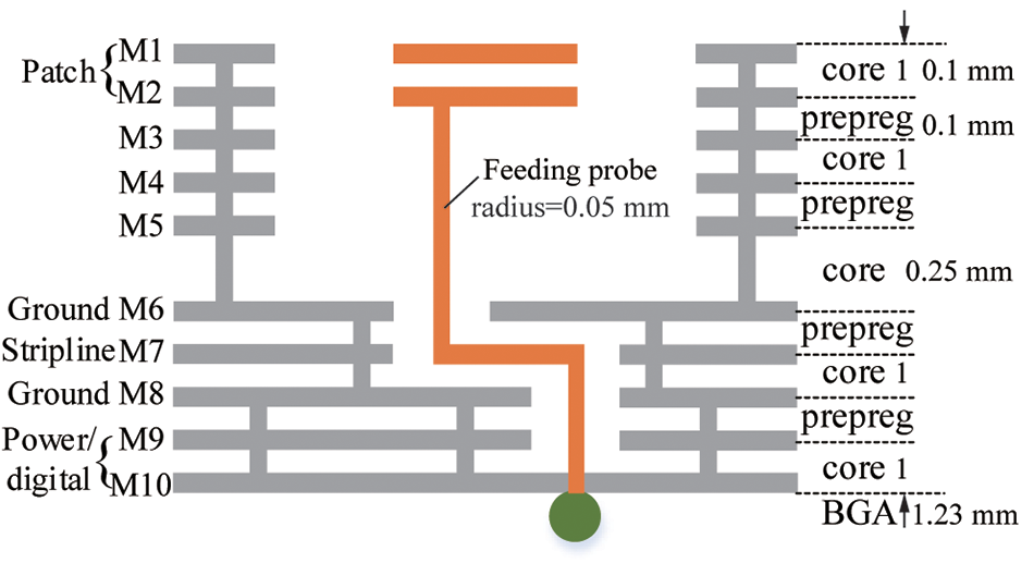
The proposed stack-up configuration of the 28 GHz patch antenna array in package on a PCB substrate is shown in Fig. 2. The package is fabricated using a 10-layer Rogers PCB, which embodies an HDI architecture. This structure is chosen to optimize performance and integration: the antenna radiating layers on top, the RF signal distribution and matching network in the middle, and the DC power and control routing layers at the bottom. The stack comprises 1 thick core layer of 0.25 mm, 4 thin core layers of 0.1 mm, and 4 prepreg layers of 0.1 mm. The thickness of copper (i.e. Mi with i = 1, 2, …, 10) is 18 µm, resulting in a total package thickness of 1.23 mm. The core and prepreg materials are Rogers RO4350 and RO4450B, respectively, both with a relative permittivity ε r of 3.66 and loss tangent tanδ of 0.004, ensuring low-loss propagation at millimeter-wave frequencies.
Stack-up configuration of a 28 GHz patch antenna array in package in PCB substrate.

Figure 2 Long description
Stack-up configuration of a 28 GHz patch antenna array in a PCB substrate. The structure includes a feeding probe with a radius of 0.05 mm. The layers are labeled from M1 to M10, with M1 to M5 designated as patch layers, M6 as ground, M7 as stripline, M8 as ground, M9 as power and M10 as digital. The stack comprises alternating core and prepreg layers: core 1 with a thickness of 0.1 mm, prepreg with a thickness of 0.1 mm, core 1 with a thickness of 0.1 mm, prepreg with a thickness of 0.1 mm, core 1 with a thickness of 0.25 mm, prepreg with a thickness of 0.1 mm, core 1 with a thickness of 0.1 mm, prepreg with a thickness of 0.1 mm and core 1 with a thickness of 0.1 mm. The total package thickness is labeled as BGA 1.23 mm.
The stacked patch antenna topology, employed for broad bandwidth consideration (i.e. over 26.5–29.5 GHz), is implemented on the upper layers. The patch antenna configuration is chosen because of its low profile, ease of fabrication and compatibility with integrated circuit technology [Reference Lee and Luk15].The size of the top patch (on layer M1) and the bottom patch (on layer M2) is 2.5 × 2.5 mm and 2.5 × 2.2 mm, respectively. The different patch sizes are chosen for enhancing the impedance bandwidth without increasing substrate thickness. Indeed, the unequal dimensions of patches create distinct resonant frequencies, with the lower patch predominantly determining the lower resonance and the upper patch the higher resonance. The electromagnetic coupling between the two patches results in a dual-resonance impedance response, when the coupling strength is optimized via the patch size ratio and substrate thickness, the two resonances merge into a broad operational bandwidth. In this design, the compression of the lower patch in the E-plane direction (2.2 mm vs. 2.5 mm) modifies the current distribution, which, together with the antiphase feeding technique, effectively suppresses cross-polarization components arising from higher-order modes [Reference Lee and Luk15].
The lower patch is fed directly by a probe with a radius of 0.05 mm. The matching network is designed on M7 in stripline configuration with solid ground planes on layers M6 and M8. Notice that layer M6 provides also effective EM shielding that isolates the sensitive antenna region from the noise and interference of the digital circuits below. The bottom-most layers, M9 and M10, are preserved for the power, analog, and digital control routing of the beamforming chip. This hierarchical layer assignment facilitates a clean separation of analog/RF and digital/power domains, which is important for maintaining signal integrity and minimizing noise coupling in a fully integrated AiP solution.
Antenna in package module design
Figure 3 (a) and (b) shows the 3D view and side view of the proposed 2 × 2 patch antenna array with packaged flip-chip BGA beamforming chip. This 2 × 2 antenna sub-array serves as the fundamental building block for constructing larger arrays. To demonstrate the scalability of this architecture, a 4 × 4 antenna array has been designed and analyzed. This larger array is constructed by tiling four identical 2 × 2 sub-arrays in a rectangular grid on the PCB. Each sub-array is driven by its own dedicated BFIC, resulting in a system with four independent beamforming chips controlling the 16 radiating elements. The antenna element spacing d is 5.2 mm, corresponding to the half wavelength in free space (i.e. 0.5λ 0) at 28 GHz, which is conventionally chosen to avoid grating lobes within the visible space for a wide range of scan angles. In this case, the grating-lobe-free steering range is theoretically ±90° in the principal planes. Indeed, for a phased array, steering the main beam to a scan angle θ scan requires a progressive phase shift between adjacent elements given in equation (1) [Reference Hansen16]. Note that, this phase shift is implemented by the BFIC:
 \begin{equation}\Delta \varphi {\text{ = }}\frac{{2\pi }}{{{\lambda _0}}}d{\text{sin(}}{\theta _{{\text{scan}}}}{\text{)}}{\text{.}}\end{equation}
The used 2 × 2 BFIC is fully integrated in a SiGe BiCMOS technology with four RF ports to steer the antenna beams. The flip-chip die consisting of 49 bump pins (pitch = 0.5 mm, diameter = 0.25 mm) attached to the bottom of the package. The entire module is assembled to a carrier PCB board using 32 BGA balls (pitch = 0.8 mm, diameter = 0.4 mm). The overall package size is 10.4 mm × 10.4 mm × 1.23 mm and 22 mm × 22 mm × 1.23 mm, respectively, for 2 × 2 and 4 × 4 arrays. Ground vias array (diameter = 0.2 mm, pitch = 0.53 mm) are placed from layer M1 to M6 along the non-radiating edges of each patch (see Fig. 3). These vias create an electromagnetic shielding barrier that suppresses reactive near-field coupling between adjacent patches and thus improve the port isolation. However, it should be noted that these vias slightly reduce the antenna bandwidth. For the 2 × 2 sub-array, ground vias are placed only along the E-plane edges to preserve bandwidth. In contrast, for the 4 × 4 array, ground vias are added along both E- and H-plane edges to further suppress coupling, where port isolation becomes essential for reliable beamforming performance. Moreover, an antiphase feeding technique is applied by exciting adjacent patch elements to the BFIC outputs with a 180° phase difference via the stripline network. This technique cancels cross-polarized fields radiated by higher-order modes of the elements [Reference Lee and Luk15].
Schematic of a 28 GHz 2 × 2 antenna in package with flip-chip BGA IC chip. (a) 3D view and (b) side view.

Figure 3 Long description
The figure shows two views of a 28 GHz antenna in package design that uses a flip chip BGA integrated circuit. Panel a is a 3D view showing a square multilayer package tilted at an angle, with four square radiating patches arranged on the top surface in orange, surrounded by ground walls along the edges. Labels point to the patch, the ground wall, the matching region, and the BF chip embedded in the structure. Panel b is a side view of the same package, showing the layered board with the ground wall and patch on the upper layers and a row of BGA balls beneath the package connecting it to the board below.
The antenna presents an inductive input impedance characteristic over the operating frequency band due to the use of probe feeding (radius = 0.05 mm). As illustrated in Fig. 4(a), the antenna feeding probe is surrounded by six ground vias extending from layer M6 to M8, forming a 50 Ω coax-like transition. The matching network connecting the BFIC’s BGA balls to the antenna feeding point consists of two stripline sections. The first matching stripline section (Z C1 = 28 Ω, electrical/physical length = 18.5°/0.19 mm) is designed to resonate with the feed inductance to transform the impedance to a pure resistance at its output. Subsequently, the second matching stripline (Z C1 = 56 Ω, electrical/physical length = 90°/0.35 mm) serves as a quarter-wave impedance transformer to convert that real resistance to 50 Ω while simultaneously compensating for the parasitic effects of the BGA balls. Based on the layer stack in Fig. 2, the stripline widths for 28 and 56 Ω are 0.28 and 0.09 mm, respectively.
These striplines are connected to the beamforming chip’s BGA balls via another coax-like transition spanning from layer M8 to M10, with a center conductor with a radius of 0.07 mm. Note that, the equivalent electrical model of the BGA balls was extracted through 3D electromagnetic simulations. As depicted in Fig. 4(b), the BGA ball is modeled by a parasitic resistance R 0 of 0.05 Ω in series with a parasitic inductance L 0 of 128 pH, and two parasitic capacitances C 0 of 30 fF connected in parallel across the structure. The characteristic impedance and electrical length of stripline sections 1 and 2 with the equivalent circuit model of BGA are summarized in Table 1. This carefully engineered matching network ensures efficient power transfer from the integrated circuit to the radiating element across the targeted frequency band.
(a) Schematic of matching network for one antenna elements and (b) equivalent circuit model.

Figure 4 Long description
The figure shows the matching network for a single antenna element in two parts. Panel a is a 3D schematic of the physical structure, with vertical cylindrical vias shown in orange representing coax like vias and vias for striplines, connected by curved horizontal traces labelled matching stripline 1 and matching stripline 2, with an arrow marking the antenna feeding point. Panel b is the equivalent circuit model, drawn as a chain of transmission line segments labelled with characteristic impedances and electrical lengths for stripline 1 and stripline 2, feeding into a load network on the right that represents the BGA, shown with resistor and capacitor elements.
Measurement resutls
The performance of the proposed beamforming AiP for both the 2 × 2 and 4 × 4 array was evaluated through full-wave electromagnetic simulation in ANSYS HFSS and subsequent experimental measurement. Photographs of the fabricated 4 × 4 AiP prototype and the measurement setup are shown in Fig. 5. The radiation performance of the fabricated antenna elements was measured in an anechoic antenna chamber shown in Fig. 5(c). The device under test (DUT) is the 4 × 4 phased array, controlled by a TMYTEK BBox™ beamforming controller [17] mounted on the rotary arm of the anechoic chamber. The controller provides the required phase and amplitude control of each input enabling far-field pattern measurement.
Photographs of the fabricated 4 × 4 AiP prototype: (a) top antenna view, (b) bottom view, and (c) measurement setup.

To characterize the standalone performance of the 4 × 4 array, the 16 antenna elements were directly fed from the M10 layer via 50 Ω microstrip feedlines terminated to SMP connectors. The microstrip line width on M10 is 0.45 mm. The AiP is symmetrically divided into four quadrants, each contains four antenna elements controlled by one BFIC, as illustrated on top antenna view in Fig. 5(a) and on bottom view in Fig. 5(b). Although the four feeding lines in one quadrant (i.e. ports P1, P2, P3, and P4) were routed differently due to spatial constraints, their electrical lengths were optimized through EM simulation to be identical, ensuring a uniform phase reference for accurate pattern measurement. Note that the simulated insertion loss of each microstrip line is approximately 1.5 dB. This loss would be de-embedded from the gain measurement results to obtain the realized gain of the standalone antenna array.
The measured return loss and isolations are presented in Fig. 6(a) and (b), respectively. The 4 × 4 array demonstrates a −10 dB bandwidth of 10% (2.6 GHz, from 26 to 28.8 GHz). The measured isolations between P1 and P3/P4 in the 4 × 4 array, represented by S 31 and S 41, is better than −23 dB across the entire operation band, mainly attributed to the use of ground via fences that effectively suppresses mutual coupling. Note that the isolation between adjacent ports P1 and P2 was not measured due to the tight space between adjacent SMP connectors while setting the RF cables. The full-wave EM simulation results show an isolation S 21 better than −20 dB within the same frequency range. In addition, the simulated active reflection coefficients for the 4 × 4 array are plotted in Fig. 6(c). The active return loss remains better than −10 dB in the operation band.
(a) Measured return loss, (b) isolations, and (c) simulated active S-parameters of the fabricated 4 × 4 AiP prototype.

Figure 6 Long description
The image A showing a line graph with the title text “Return Loss (dB)” on the vertical axis and “Frequency(GHz)” on the horizontal axis. The horizontal axis runs from 24 to 32 with tick marks at 24, 25, 26, 27, 28, 29, 30, 31 and 32. The vertical axis runs from 0 at the top down to minus 50 at the bottom, with tick marks at 0, minus 10, minus 20, minus 30, minus 40 and minus 50. A legend lists six series: “S11 sim.”, “S11 meas.”, “S22 sim.”, “S22 meas.”, “S33 sim.”, “S33 meas.”. All six curves start near about minus 5 to minus 10 around 24, drop to minima between about 26 and 28, then rise toward about minus 5 to 0 by about 31 to 32. The “S11 meas.” curve reaches a minimum near about 27 at roughly minus 35. The “S22 meas.” curve reaches a minimum near about 27 at roughly minus 30. The “S33 meas.” curve reaches a minimum near about 27 at roughly minus 50. The image B showing a line graph with the vertical axis labeled “Isolation (dB)” and the horizontal axis labeled “Frequency(GHz)”. The horizontal axis runs from 24 to 32 with tick marks at 24 through 32 in steps of 1. The vertical axis runs from minus 10 at the top down to minus 60 at the bottom, with tick marks at minus 10, minus 20, minus 30, minus 40, minus 50 and minus 60. A legend lists six series: “S31 sim.”, “S31 meas.”, “S41 sim.”, “S41 meas.”, “S21 sim.”, “S23 sim.”. The curves vary across the band with multiple dips. The “S31 meas.” curve shows a deep dip near about 26.5 to 27 reaching roughly minus 45, then rises toward about minus 25 to minus 20 around 29 to 30, then drops again toward about minus 45 by about 32. The “S41 meas.” curve stays around roughly minus 20 to minus 30 from about 24 to 30, then drops toward about minus 45 by about 32. The “S21 sim.” curve is around roughly minus 20 to minus 30 from about 24 to 30, then drops toward about minus 45 by about 32. The “S23 sim.” curve is around roughly minus 25 to minus 35 from about 24 to 30, then drops toward about minus 45 by about 32. The image C showing a line graph with the vertical axis labeled “Active S-parameters(dB)” and the horizontal axis labeled “Frequency(GHz)”. The horizontal axis runs from 24 to 32 with tick marks at 24 through 32 in steps of 1. The vertical axis runs from 0 at the top down to minus 40 at the bottom, with tick marks at 0, minus 10, minus 20, minus 30 and minus 40. A legend lists multiple series labeled “S11”, “S22”, “S33”, “S44”, “S55”, “S66”, “S77” and “S88”, each shown with a distinct line style and marker. All curves form broad V-shaped responses with minima between about 27 and 29, then rise toward about minus 5 to 0 by about 31 to 32. Several curves reach minima near about 27.5 to 28.5 between roughly minus 20 and minus 35, with the deepest minima approaching about minus 40.
Performance comparison between proposed antenna and reported works in references

Table 2 Long description
The table compares the proposed antenna against four referenced works across eight columns: reference, antenna type, process technology, center frequency in GHz, dimensions in wavelengths cubed, peak gain in dBi, bandwidth in GHz, and cross polarization in dB. Reference 4 is an organic substrate patch at 28 GHz with a peak gain of 10.7 dBi. Reference 6 is a PCB patch at 26.7 GHz with a peak gain of 31 dBi achieved with power amplification. Reference 8 is a PCB dipole two by two array at 28 GHz with a peak gain of 9.5 dBi. Reference 12 is an LTCC dipole four by four array at 28 GHz with a simulated peak gain of 16.8 dBi. This work presents two PCB patch designs: a two by two array at 28 GHz with a peak gain of 9.3 dBi and cross polarization below minus 40 dB, and a four by four array at 27.5 GHz with a peak gain of 15.1 dBi. A footnote notes that starred gain values use power amplification and double starred values are simulation results.
* Gain with power amplification.
** Simulation results.
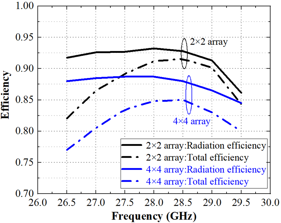
The total antenna efficiency for both arrays is plotted in Fig. 7. The 2 × 2 array exhibits a high total efficiency, exceeding 82% across the band and reaching 90% at 28 GHz. The 4 × 4 array shows a decrease in efficiency, primarily due to increased dielectric and conductor losses associated with the larger aperture and more complex feed network, yet it remains above 78% with a peak efficiency of 85% at 28.5 GHz.
Measured efficiencies for both 2 × 2 and 4 × 4 AiP array.

Figure 7 Long description
Efficiency Legend: 2 times 2 array: Radiation efficiency 2 times 2 array: Total efficiency 4 times 4 array: Radiation efficiency 4 times 4 array: Total efficiency Horizontal axis label: Frequency (Gigahertz) Horizontal axis range: 26.0 to 30.0 Vertical axis label: Efficiency Vertical axis range: 0.70 to 1.00 2 times 2 array: Radiation efficiency (26.0, 0.91), (26.5, 0.92), (27.0, 0.92), (27.5, 0.92), (28.0, 0.93), (28.5, 0.93), (29.0, 0.92), (29.5, 0.88), (30.0, 0.85) 2 times 2 array: Total efficiency (26.0, 0.82), (26.5, 0.84), (27.0, 0.86), (27.5, 0.88), (28.0, 0.90), (28.5, 0.92), (29.0, 0.91), (29.5, 0.87), (30.0, 0.83) 4 times 4 array: Radiation efficiency (26.0, 0.88), (26.5, 0.88), (27.0, 0.88), (27.5, 0.88), (28.0, 0.88), (28.5, 0.88), (29.0, 0.87), (29.5, 0.85), (30.0, 0.83) 4 times 4 array: Total efficiency (26.0, 0.76), (26.5, 0.78), (27.0, 0.80), (27.5, 0.82), (28.0, 0.84), (28.5, 0.85), (29.0, 0.85), (29.5, 0.83), (30.0, 0.80).
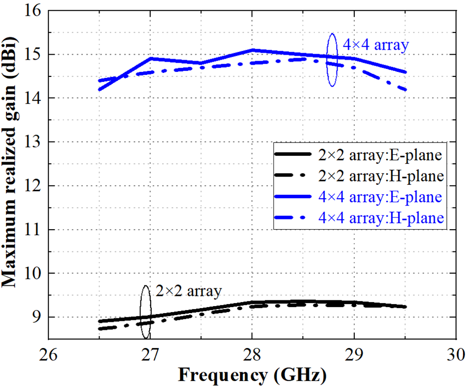
The measured maximum realized gain for the both proposed antenna arrays in package on both E and H-plane is plotted in Fig. 8. For 2 × 2 array, the maximum realized gain varies from 8.7 to 9.3 dBi within the frequency band of 26.5–29.5 GHz. At 28 GHz, the maximum realized gain in E-plane and H-plane is 9.3 and 9.2 dBi, respectively. The 4 × 4 array achieves a measured peak broadside gain of approximately 15.1 and 14.8 dBi, respectively on E- and H-plane, at 28 GHz.
Measured maximum realized gain for both 2 × 2 and 4 × 4 AiP array.

The measured co- and cross-polarized radiation patterns for the 4 × 4 array at 28 GHz are shown in Fig. 9(a). Note that, for E-plane and H-plane, the cross-polarization levels are suppressed to below −20 dB, a direct result of the implemented antiphase feeding technique. Theoretically, with four times the number of elements, the 4 × 4 array should provide an ideal theoretical gain increase of approximately 6 dBi over the 2 × 2 array (i.e. around 15 dBi instead of 13.6 dBi). In fact, the gain difference was expected since the insertion loss provided by the microstrip line was not de-embedded during the measurement. This can be deduced from Fig. 9(b), which shows the simulated 3D radiation pattern at broadside without the impact of microstrip lines, a simulated peak gain of 16.2 dBi was obtained.
(a) Measured radiation patterns for 2 × 2 and 4 × 4 AiP array at 28 GHz and (b) simulated realized gain for 4 × 4 array at 28 GHz.

Figure 9 Long description
The image A showing two polar plots labeled 2 times 2 and 4 times 4. Angle markings around each polar plot are labeled 0, 30, 60, 90, 120, 150, 180, 210, 240, 270, 300 and 330. Radial tick labels shown on the polar grids include 0, minus 20 and minus 40. Each polar plot has four traces identified by a legend: E plane Co pol, E plane X pol, H plane Co pol and H plane X pol. The 2 times 2 polar plot shows the co pol traces forming a broad main lobe with the largest radius near 0 degrees and 330 degrees and a reduced radius near 180 degrees. The x pol traces remain closer to the center than the co pol traces across most angles. The 4 times 4 polar plot shows the co pol traces forming a broad main lobe with the largest radius near 0 degrees and 330 degrees and a reduced radius near 180 degrees. The x pol traces remain closer to the center than the co pol traces across most angles. The image B showing a line graph with x-axis label Theta(Degree) and y-axis label Realized Gain(dB). The x-axis ranges from minus 150 to 150 with labeled ticks at minus 150, minus 100, minus 50, 0, 50, 100 and 150. The y-axis ranges from minus 30 to 20 with labeled ticks at minus 30, minus 20, minus 10, 0, 10 and 20. A legend lists two series: E plane and H plane. The E plane curve rises to a peak near theta equals 0 at about 16 decibel, then drops to deep nulls near theta around minus 50 and plus 50 at about minus 20 decibel, then returns to around 0 to 5 decibel near theta around minus 30 and plus 30 and decreases toward negative values approaching theta near minus 150 and plus 150. The H plane curve follows a similar shape with a peak near theta equals 0 at about 16 decibel, deep nulls near theta around minus 50 and plus 50 at about minus 20 decibel and lower values toward theta near minus 150 and plus 150, reaching about minus 25 to minus 30 decibel near the ends.
The measured co- and cross-polarized radiation patterns for both 2 × 2 and 4 × 4 arrays at 28 GHz are shown in Fig. 9(a). The 2 × 2 array achieves a peak realized gain of 9.3 dBi with a cross-polarization level below −40 dB, thanks to the antiphase feeding technique. For the 4 × 4 array, the measured peak gain is 15.1 dBi, which already accounts for the 1.5 dB insertion loss of the microstrip feed lines during the measurement. The cross-polarization level of the 4 × 4 array remains below −20 dB across the main beam. Figure 9(b) presents the simulated E- and H-plane patterns of the 4 × 4 array without feed lines, showing a peak gain of 16.2 dBi, which agrees well with the simulated value. It is observed that the measured co-polarized pattern of the 4 × 4 array exhibits a slightly broader main beam than the simulated one. This discrepancy is most likely attributed to measurement tolerances, in particular residual phase and amplitude errors among the 16 elements due to connector and cable variations, which cannot be perfectly calibrated.
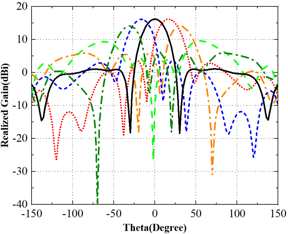
The beam-steering capability of the 4 × 4 array at 28 GHz is demonstrated in Fig. 10. The beam steering of the antenna array was realized by setting a phase shifting in both x- and y-direction, the achieved −3 dB scanning range for the 4 × 4 array is approximately ±40° in both planes. Performance comparisons with state-of-the-art designs are summarized in Table 2. It can be seen that the proposed AiP achieves high gain and wide bandwidth, together with superior cross-polarization suppression (<−40 dB for the 2 × 2 array) in a compact form factor, and low cost enabled by scalable HDI PCB process.
Beam scanning performance of 4 × 4 AiP array.

Figure 10 Long description
Realized Gain (dBic) Single plot with multiple overlaid curves. The horizontal axis is labeled Theta(Degree), ranging from minus 150 to 150, with labeled ticks at minus 150, minus 100, minus 50, 0, 50, 100 and 150. The vertical axis is labeled Realized Gain(dBic), ranging from minus 40 to 20, with labeled ticks at minus 40, minus 30, minus 20, minus 10, 0, 10 and 20. Theta is shown as an angle in degrees. Realized gain is shown in dBic. Multiple curves are drawn with different line styles, but no legend text is visible to map each curve to a named condition. The curves form radiation-pattern-like lobes with several local maxima and multiple narrow nulls. Several peaks rise to near 20 dBic, with prominent peaks occurring around the central region near 0 degrees and additional peaks at off-center angles. Several nulls drop sharply toward the bottom of the axis, with the deepest visible nulls reaching close to minus 40 dBic at multiple theta positions across the sweep. The curves intersect at multiple theta values and several curves show broad humps spanning tens of degrees with superimposed sharp notches.
Conclusion
This paper has presented a detailed design and experimental validation of a highly integrated, scalable stacked patch AiP solution for 28 GHz 5G/6G systems. The work successfully demonstrates a low-cost approach utilizing a standard 10-layer organic HDI PCB substrate. Through codesign and full-wave optimization of the antenna elements, stripline matching networks, and coaxial-style transitions, the fabricated 2 × 2 AiP module exhibits a 15% fractional bandwidth (25.9–30.3 GHz), a peak realized gain of 9.3 dBi, a total efficiency exceeding 90%, and a low cross-polarization level below −40 dB at 28 GHz. The 4 × 4 AiP array performance aligns with theoretical expectations, achieving a peak gain of over 15.1 dBi while maintaining a high radiation efficiency. The measured port isolation of better than −20 dB confirms the effectiveness of the grounding and isolation strategies. This work conclusively validates the proposed HDI PCB-based AiP architecture as a viable, cost-effective, and highly scalable platform for medium-to-large-scale phased arrays. The demonstrated methodology, from a core 2 × 2 module to a functional 4 × 4 array, provides a clear and reliable pathway for implementing even larger systems, such as 256-element arrays for base station applications, by leveraging embedded power dividers within the multilayer PCB board.
Funding statement
This work was supported in part by National Natural Science Foundation of China (NSFC) under Grant No. 62404055, in part by Jiangxi Natural Science Foundation of Jiangxi under Grant No. 20252BAC240229 and in part by Doctoral Research Startup Fund of Gannan University of Science and Technology.
Competing interests
The author(s) declare none.

Xiao-Lan Tang received her Ph.D. degree in Optics and Radio Frequency from University of Grenoble in 2013. She is now associate professor at Gannan University of Science and Technogly. Her main research interests are millimeter wave antennas design and silicon-based microwave power amplifiers design.

Yong Xu is a deputy research director at Guangdong Greater Bay Area Institute of Integrated Circuit and System, Guangzhou, China. He received his M.S. and Ph.D. in microelectronics from the Grenoble Institute of Technology, Grenoble, France, in 2008 and 2011, respectively. He was a research associate (2011–2013) at National Institute for Materials Science, Tsukuba, Japan, an assistant professor (2013–2018) at Dongguk University, Seoul, South Korea, and a professor (2018–2025) at Nanjing University of Posts and Telecommunications, Nanjing, China. His research interest lies in semiconductor devices, in particular, the related device physics.

Zhang Ju Hou received the M.S. degree and the Ph.D. degree in electronic engineering from the City University of Hong Kong in 2014 and 2018, respectively. He is currently a Senior Engineer of the Millimeter-Wave and Terahertz Circuits and Antennas in Pengcheng laboratory. His current research interests include antenna-in-package (AiP) design, millimeter-wave and sub-terahertz technologies in 5G/6G, and biomedical applications.