2. LB model with self-tuning EOS

For the sake of completeness, the recent multiphase LB model with a self-tuning EOS is briefly introduced in this section, and the reader is referred to previous works (Huang, Wu & Adams Reference Huang, Wu and Adams2019a; Huang et al. Reference Huang, Wu and Adams2019c; Huang, Lan & Li Reference Huang, Lan and Li2020) for more details. The LB equation for the density distribution function $f_i (\boldsymbol {x}, t)$ can be written as (Huang et al. Reference Huang, Wu and Adams2019a)

(2.1a)\begin{gather} f_i (\boldsymbol{x} + \boldsymbol{e}_i \delta_t, t +\delta_t) = \bar{f}_i (\boldsymbol{x}, t) , \end{gather}

(2.1b)\begin{gather}\bar{\boldsymbol{m}} (\boldsymbol{x}, t) = \boldsymbol{m} + \delta_t \boldsymbol{F}_m - \boldsymbol{\mathsf{S}} \left( \boldsymbol{m} - \boldsymbol{m}^\textit{eq} + \frac{\delta_t}{2} \boldsymbol{F}_m \right) + \boldsymbol{\mathsf{S}} \boldsymbol{Q}_m , \end{gather}

where (2.1a) is the linear streaming process in velocity space, (2.1b) is the local collision process in moment space at position $\boldsymbol {x}$ and time $t$ and the overbar denotes the post-collision state. In the streaming process, ${\boldsymbol{e}}_i$ is the discrete velocity and $\delta_t$ is the time step. In the collision process, $\boldsymbol{\mathsf{S}}$ is the collision matrix, $\boldsymbol {m}^\textit {eq}$ is the equilibrium moment, $\boldsymbol {F}_m$ is the discrete force and $\boldsymbol {Q}_m$ is the third-order compensation term for the third-order discrete lattice effect. The transformations between velocity and moment spaces can be expressed as $\boldsymbol {m} = \boldsymbol{\mathsf{M}} (f_i)^\mathrm {T}$ and $(\bar {f}_i)^\mathrm {T} = \boldsymbol{\mathsf{M}} ^{-1} \bar {\boldsymbol {m}}$, where $\boldsymbol{\mathsf{M}}$ is the orthogonal transformation matrix and $(f_i)^\mathrm {T}$ is a short notation of the lattice vector $( f_0, f_1, \ldots, f_{N-1} )^\mathrm {T}$ with $N$ the number of discrete velocities. The macroscopic density $\rho$ and momentum $\rho \boldsymbol {u}$ are defined as

(2.2a,b)\begin{equation} \rho = \sum_{i=0}^{N-1} f_i , \quad \rho \boldsymbol{u} = \sum_{i=0}^{N-1} \boldsymbol{e}_i f_i + \frac{\delta_t}{2} \boldsymbol{F} , \end{equation}

where $\boldsymbol {F}$ is the total force consisting of the external force $\boldsymbol {F}_\textit {ext}$ such as gravity and the pairwise interaction force $\boldsymbol {F}_\textit {pair}$ for multiphase dynamics, i.e. $\boldsymbol {F} = \boldsymbol {F}_\textit {ext} + \boldsymbol {F}_\textit {pair}$. The nearest-neighbour interaction is considered in this work and thus the pairwise interaction force can be written as

(2.3)\begin{equation} \boldsymbol{F}_\textit{pair} = G^2 \rho (\boldsymbol{x}) \sum_{i=1}^{N-1} \omega (| \boldsymbol{e}_i \delta_t |^2) \rho (\boldsymbol{x} + \boldsymbol{e}_i \delta_t) \boldsymbol{e}_i \delta_t , \end{equation}

where $G^2$ controls the interaction strength and $\omega (| \boldsymbol {e}_i \delta _t |^2)$ is the distance-dependent weight to maximize the isotropy degree of $\boldsymbol {F}_\textit {pair}$.

Without loss of generality, the two-dimensional LB model based on the standard two-dimensional nine-velocity (D2Q9) discrete velocity set ($N = 9$) is considered. The nine discrete velocities are (Qian, d'Humières & Lallemand Reference Qian, d'Humières and Lallemand1992)

(2.4)\begin{equation} \boldsymbol{e}_i = \begin{cases} c ( 0 ,\ 0 )^\mathrm{T}, & i=0, \\ c ( \cos[(i-1){\rm \pi}/2] , \sin[(i-1){\rm \pi}/2] )^\mathrm{T}, & i=1 \sim 4, \\ \sqrt{2}c ( \cos[(2i-1){\rm \pi}/4] , \sin[(2i-1){\rm \pi}/4] )^\mathrm{T}, & i=5 \sim 8, \\ \end{cases} \end{equation}

where the lattice speed $c = \delta _x / \delta _t$. The corresponding orthogonal transformation matrix is (Lallemand & Luo Reference Lallemand and Luo2000)

(2.5)\begin{equation} \boldsymbol{\mathsf{M}} = \begin{bmatrix} 1 & 1 & 1 & 1 & 1 & 1 & 1 & 1 & 1 \\ -4 & -1 & -1 & -1 & -1 & 2 & 2 & 2 & 2 \\ 4 & -2 & -2 & -2 & -2 & 1 & 1 & 1 & 1 \\ 0 & 1 & 0 & -1 & 0 & 1 & -1 & -1 & 1 \\ 0 & -2 & 0 & 2 & 0 & 1 & -1 & -1 & 1 \\ 0 & 0 & 1 & 0 & -1 & 1 & 1 & -1 & -1 \\ 0 & 0 & -2 & 0 & 2 & 1 & 1 & -1 & -1 \\ 0 & 1 & -1 & 1 & -1 & 0 & 0 & 0 & 0 \\ 0 & 0 & 0 & 0 & 0 & 1 & -1 & 1 & -1 \end{bmatrix} . \end{equation}

For the LB model with self-tuning EOS, the conventional diagonal collision matrix is modified to a non-diagonal one to ensure that the Newtonian viscous stress can be correctly recovered (Huang et al. Reference Huang, Wu and Adams2019c)

(2.6)\begin{equation} \boldsymbol{\mathsf{S}} = \begin{bmatrix} s_0 & 0 & 0 & 0 & 0 & 0 & 0 & 0 & 0\\ 0 & s_e & k s_\varepsilon \omega_e & 0 & h \hat{u}_x s_q \omega_e & 0 & h \hat{u}_y s_q \omega_e & 0 & 0\\ 0 & 0 & s_\varepsilon & 0 & 0 & 0 & 0 & 0 & 0\\ 0 & 0 & 0 & s_j & 0 & 0 & 0 & 0 & 0\\ 0 & 0 & 0 & 0 & s_q & 0 & 0 & 0 & 0\\ 0 & 0 & 0 & 0 & 0 & s_j & 0 & 0 & 0\\ 0 & 0 & 0 & 0 & 0 & 0 & s_q & 0 & 0\\ 0 & 0 & 0 & 0 & 2 b \hat{u}_x s_q \omega_p & 0 & -2 b \hat{u}_y s_q \omega_p & s_p & 0\\ 0 & 0 & 0 & 0 & b \hat{u}_y s_q \omega_p & 0 & b \hat{u}_x s_q \omega_p & 0 & s_p\\ \end{bmatrix}, \end{equation}

where $\hat {\boldsymbol {u}} \equiv (\hat {u}_x, \hat {u}_y)^\mathrm {T} = \boldsymbol {u} / c$, $\omega _{e,p} \equiv s_{e,p}/2 - 1$ and $k$, $h$ and $b$ are coefficients determined by (2.11a–d). To achieve the self-tuning EOS, the equilibrium moment is set to

(2.7)\begin{align} \boldsymbol{m}^\textit{eq} &= [ \rho , -2 \rho + 2 \eta + 3 \rho |\hat{\boldsymbol{u}}|^2 , \rho + \beta_\varepsilon \eta - 3 \rho |\hat{\boldsymbol{u}}|^2 , \rho \hat{u}_x , -\rho \hat{u}_x , \rho \hat{u}_y ,\nonumber\\ &\quad -\rho \hat{u}_y , \rho \hat{u}_x^2 - \rho \hat{u}_y^2 , \rho \hat{u}_x \hat{u}_y ]^\mathrm{T} , \end{align}

where $\eta$ is a built-in variable in the recovered EOS and $\beta _\varepsilon$ is a coefficient determined by (2.11a–d). The corresponding discrete force is

(2.8)\begin{equation} \boldsymbol{F}_m = [ 0 , 6 \hat{\boldsymbol{F}} \boldsymbol{\cdot} \hat{\boldsymbol{u}} , -6 \hat{\boldsymbol{F}} \boldsymbol{\cdot} \hat{\boldsymbol{u}} , \hat{F}_x , -\hat{F}_x , \hat{F}_y , -\hat{F}_y , 2 \hat{F}_x \hat{u}_x - 2 \hat{F}_y \hat{u}_y , \hat{F}_x \hat{u}_y + \hat{F}_y \hat{u}_x ]^\mathrm{T} , \end{equation}

where $\hat {\boldsymbol {F}} \equiv ( \hat {F}_x, \hat {F}_y)^\mathrm {T}= \boldsymbol {F} / c$. The third-order compensation term for the third-order discrete lattice effect can be written as (Huang et al. Reference Huang, Wu and Adams2019a)

(2.9)\begin{equation} \boldsymbol{Q}_m = \frac{G^2 \delta_x^2 \delta_t^2}{12} [ 0 , 6 |\boldsymbol{\nabla} \rho|^2 , -6 |\boldsymbol{\nabla} \rho|^2 , 0 , 0 , 0 , 0 , (\mathrm{\partial}_x \rho)^2 - (\mathrm{\partial}_y \rho)^2 , (\mathrm{\partial}_x \rho) (\mathrm{\partial}_y \rho) ]^\mathrm{T} . \end{equation}

Following the idea of Huang et al. (Reference Huang, Wu and Adams2019a), an improved local scheme can be proposed for the $\boldsymbol {\nabla } \rho$ in $\boldsymbol {Q}_m$ as

(2.10)\begin{equation} \boldsymbol{\nabla} \rho = \frac{ \boldsymbol{F}_\textit{pair} + \dfrac23 \boldsymbol{F}_\textit{ext}}{ G^2 \delta_x^2 \rho + \dfrac23 \left( \dfrac{\mathrm{\partial} p_\textit{EOS} }{\mathrm{\partial} \rho} \right)_T } . \end{equation}

Here, $p_\textit {EOS}$ denotes the specified EOS for multiphase fluids in real applications, and thus the expression for $( {\mathrm {\partial } p_\textit {EOS} }/{\mathrm {\partial } \rho } )_T$ is known.

Through the second-order Chapman–Enskog analysis, the coefficients in $\boldsymbol{\mathsf{S}}$ and $\boldsymbol {m}^\textit {eq}$ should satisfy (Huang et al. Reference Huang, Wu and Adams2019c)

(2.11a–d)\begin{equation} k = 1-\varpi ,\quad h = \frac{6 \varpi (1-\varpi)}{1-3\varpi} ,\quad b = \frac{1-\varpi}{1-3\varpi} ,\quad \beta_\varepsilon ={-}\frac{2}{1-\varpi} . \end{equation}

Here, the coefficient $\varpi$ is related to the bulk viscosity. Through the third-order Chapman–Enskog analysis, the relaxation parameters in $\boldsymbol{\mathsf{S}}$ should satisfy (Huang et al. Reference Huang, Wu and Adams2019c)

(2.12)\begin{equation} \left( \frac{1}{s_p} - \frac12 \right) \left( \frac{1}{s_q} - \frac12 \right) = (k+1) \left( \frac{1}{s_e} - \frac12 \right) \left( \frac{1}{s_q} - \frac12 \right) = \frac{1}{12} . \end{equation}

Combining the second- and third-order Chapman–Enskog analyses, the following mass–momentum conservation equations can be recovered

(2.13a)\begin{equation} \left. \begin{array}{c@{}} \mathrm{\partial}_t \rho + \boldsymbol{\nabla} \boldsymbol{\cdot} (\rho \boldsymbol{u}) = 0, \\ \mathrm{\partial}_t (\rho \boldsymbol{u}) + \boldsymbol{\nabla} \boldsymbol{\cdot} (\rho \boldsymbol{u} \boldsymbol{u}) ={-}\boldsymbol{\nabla} \boldsymbol{\cdot} \boldsymbol{\mathsf{P}} + \boldsymbol{F}_\textit{ext} + \boldsymbol{\nabla} \boldsymbol{\cdot} \boldsymbol{\varPi} , \end{array}\right\} \end{equation}

where the Newtonian viscous stress $\boldsymbol {\varPi }$ and pressure tensor $\boldsymbol{\mathsf{P}}$ are given as

(2.13b)\begin{gather} \boldsymbol{\varPi} = \rho \nu [\boldsymbol{\nabla} \boldsymbol{u} + (\boldsymbol{\nabla} \boldsymbol{u})^\mathrm{T} - (\boldsymbol{\nabla} \boldsymbol{\cdot} \boldsymbol{u}) \boldsymbol{\mathsf{I}}] + \rho \varsigma (\boldsymbol{\nabla} \boldsymbol{\cdot} \boldsymbol{u}) \boldsymbol{\mathsf{I}} , \end{gather}

(2.13c)\begin{gather}\boldsymbol{\mathsf{P}} = \left( p_\textit{EOS} - \kappa \rho \boldsymbol{\nabla} \boldsymbol{\cdot} \boldsymbol{\nabla} \rho - \frac{\kappa}{2} \boldsymbol{\nabla} \rho \boldsymbol{\cdot} \boldsymbol{\nabla} \rho \right) \boldsymbol{\mathsf{I}} + \kappa \boldsymbol{\nabla} \rho \boldsymbol{\nabla} \rho . \end{gather}

Here, the kinematic and bulk viscosities are $\nu = c_s^2 \delta _t ( s_p^{-1} - 1/2 )$ and $\varsigma = \varpi c_s^2 \delta _t ( s_e^{-1} - 1/2 )$, respectively, with $c_s = c \big / \sqrt {3}$ the lattice sound speed, the multiphase EOS is $p_\textit {EOS} = p_{\textit {LBE}} - G^2 \delta _x^2 \rho ^2 / 2$ with $p_{\textit {LBE}} = c_s^2 (\rho + \eta )$ the self-tuning EOS intrinsically recovered by the LB equation (i.e. by its collision operator without the force term) and the gradient energy coefficient is $\kappa = G^2 \delta _x^4 / 4$. Note that there are some additional cubic terms of velocity in recovering the Newtonian viscous stress, which are here ignored under the low lattice Mach number condition and can be eliminated by trivial modifications (see Appendix A). The intrinsically recovered EOS $p_{\textit {LBE}}$ is a non-ideal-gas EOS that can be self-tuned via the built-in variable $\eta$. It can be physically interpreted as the incorporation of the short-range repulsive molecular interaction, because the physical short-range repulsive core is actually the volume-exclusion effect of finite-size molecules and can be well modelled by Enskog theory for dense gases (He & Doolen Reference He and Doolen2002). The present incorporation of the repulsive molecular interaction is significantly different from the multirange pseudopotential LB model, where the repulsive interaction is associated with the nearest-neighbour interaction (Falcucci et al. Reference Falcucci, Bella, Chiatti, Chibbaro, Sbragaglia and Succi2007). Such repulsive interaction is middle range rather than short range. The self-tuning EOS in the present work means that the intrinsically recovered EOS can be tuned itself without resorting to the force term, as done in previous LB models. It should not be confused with the self-tuning strategy proposed by Colosqui et al. (Reference Colosqui, Falcucci, Ubertini and Succi2012) to generate a customized EOS for multiphase fluids. Such a self-tuning strategy of a customized EOS can be directly plugged into the present LB model, where the multiphase EOS can be arbitrarily specified. Moreover, the self-tuning EOS distinguishes the present LB model from previous LB models, and it should also not be confused with the arbitrary specification of a realistic multiphase EOS in real applications.

In this work, the multiphase EOS combining the Carnahan–Starling expression for hard spheres (Carnahan & Starling Reference Carnahan and Starling1969) with an attractive term is taken as an example

(2.14)\begin{equation} p_\textit{EOS} = K_\textit{EOS} \left[ \rho R T \frac{ 1 + \tilde{b} \rho /4 + (\tilde{b} \rho /4)^2 - (\tilde{b} \rho /4)^3 }{ (1 - \tilde{b} \rho /4)^3 } - \tilde{a} \rho^2 \right] , \end{equation}

where the coefficients $\tilde {a}$ and $\tilde {b}$ are determined by the critical temperature $T_\textit {cr}$ and pressure $p_\textit {cr}$ as $\tilde {a} = 0.4963880577294099 R^2 T_\textit {cr}^2 / p_\textit {cr}$ and $\tilde {b} = 0.1872945669467330 R T_\textit {cr} / p_\textit {cr}$. The interaction strength is then set to (Huang et al. Reference Huang, Wu and Adams2019c)

(2.15)\begin{equation} G = K_\textit{INT} \sqrt{2 K_\textit{EOS} \tilde{a} \big/ \delta_x^2 }, \end{equation}

and the lattice sound speed is chosen as

(2.16)\begin{equation} c_s = K_\textit{INT} \left.\sqrt{ \left( \frac{ \mathrm{\partial} p_\textit{EOS} }{ \mathrm{\partial} \rho } \right)_T + 2 K_\textit{EOS} \tilde{a} \rho } \right|_{\rho = \rho_l } . \end{equation}

In (2.14), (2.15) and (2.16), the scaling factors $K_\textit {EOS}$ and $K_\textit {INT}$ are introduced to independently adjust the liquid–gas surface tension $\sigma _{lg}$ and liquid–gas interface thickness $W_{lg}$, which satisfy $\sigma _{lg} \propto K_\textit {EOS} K_\textit {INT}$ and $W_{lg} \propto K_\textit {INT}$, respectively. For the multiphase EOS, the liquid and gas phases are distinguishable below the critical point, above which only one phase, called the supercritical fluid, exists. Thus, the reduced temperature $T_r = T / T_\textit {cr}$ is commonly introduced to represent the state with respect to the critical point. By definition, both the liquid and gas phases are compressible to some extent, and a realistic multiphase EOS can ensure that the isothermal compressibility $({1}/{\rho }) ( {\mathrm {\partial } \rho }/{\mathrm {\partial } p_\textit {EOS} } )_T$ for the liquid phase is much smaller than that for the gas phase. Moreover, the pressure determined by the multiphase EOS is thermodynamic rather than hydrodynamic. As shown by (2.16), the lattice sound speed is associated with the multiphase EOS, and thus the usual low lattice Mach number condition (evaluated with the lattice sound speed) also implies the weakly compressible flows in physics. In the following theoretical and numerical calculations, the basic parameters are chosen as $\varpi = 1/6$, $\delta _x =1$, $\tilde {a} = 1$, $\tilde {b} = 4$, $R = 1$, $\sigma _{lg} = 0.01$ and $W_{lg} = 10$ unless otherwise stated. The reduced temperature $T_r$ is set to $0.8$, which is low enough for the present study to show the large deviation between the fluid densities on the solid surface and in the bulk phase (see figure 3). Thus, the liquid-to-gas density ratio is approximately $15$, and the scaling factors are $K_\textit {EOS} = 0.479820$ and $K_\textit {INT} = 2.294922$.

3. Surface thermodynamics

In this section, the surface thermodynamics for multiphase flows is theoretically explored and a new free-energy density for the solid surface will be proposed. For a multiphase system involving a solid surface, the free-energy functional can be written as

(3.1)\begin{equation} {\varPsi} = \int_V \left( \psi_b + \frac{\kappa}{2} |\boldsymbol{\nabla} \rho|^2 \right) \, \mathrm{d} V + \int_A \psi_s \, \mathrm{d} A , \end{equation}

where $\psi _b$ is the bulk free-energy density, $({\kappa }/{2}) | \boldsymbol {\nabla } \rho |^2$ is the free-energy density for the phase interface, $\psi _s$ is the free-energy density for the solid surface, $V$ is the domain occupied by the multiphase fluids and $A$ is the boundary of $V$ (i.e. $A$ is the solid surface). The first variation of ${\varPsi }$ is

(3.2)\begin{equation} \delta {\varPsi} = \int_V \delta \mspace{-1.0mu} \rho \left( \frac{\mathrm{\partial} \psi_b}{\mathrm{\partial} \rho} - \kappa \boldsymbol{\nabla} \boldsymbol{\cdot} \boldsymbol{\nabla} \rho \right) \, \mathrm{d} V + \int_A \delta \mspace{-1.0mu} \rho_s \left( \kappa \boldsymbol{\nabla} \rho \boldsymbol{\cdot} \hat{\boldsymbol{n}}_s + \frac{\mathrm{\partial} \psi_s}{ \mathrm{\partial} \rho_s } \right) \, \mathrm{d} A , \end{equation}

where $\hat {\boldsymbol {n}}_s$ is the outward unit normal vector of the solid surface, $\rho _s$ denotes the fluid density on the solid surface and $\delta \mspace {-1.0mu} \rho$ and $\delta \mspace {-1.0mu} \rho _s$ are the variations of $\rho$ and $\rho _s$, respectively. Note that $\rho _s \equiv \rho |_A$ and $\delta \mspace {-1.0mu} \rho _s \equiv \delta \mspace {-1.0mu} \rho |_A$ since $A$ is the boundary of $V$. According to (3.2), a chemical potential can be introduced as $\mu = {\mathrm {\partial } \psi _b}/{ \mathrm {\partial } \rho } - \kappa \boldsymbol {\nabla } \boldsymbol {\cdot } \boldsymbol {\nabla } \rho$, and then the pressure tensor, defined as $\boldsymbol {\nabla } \boldsymbol {\cdot } \boldsymbol{\mathsf{P}} = \rho \boldsymbol {\nabla } \mu$, can be obtained

(3.3)\begin{equation} \boldsymbol{\mathsf{P}} = \left( \rho \frac{\mathrm{\partial} \psi_b}{\mathrm{\partial} \rho} - \psi_b - \kappa \rho \boldsymbol{\nabla} \boldsymbol{\cdot} \boldsymbol{\nabla} \rho - \frac{\kappa}{2} \boldsymbol{\nabla} \rho \boldsymbol{\cdot} \boldsymbol{\nabla} \rho \right) \boldsymbol{\mathsf{I}} + \kappa \boldsymbol{\nabla} \rho \boldsymbol{\nabla} \rho , \end{equation}

which indicates that the multiphase EOS satisfies $p_\textit {EOS} = \rho {\mathrm {\partial } \psi _b}/{\mathrm {\partial } \rho } - \psi _b$. Unlike previous works in which a simple bulk free-energy density is adopted (Connington & Lee Reference Connington and Lee2013; Connington, Lee & Morris Reference Connington, Lee and Morris2015; Fakhari & Bolster Reference Fakhari and Bolster2017; He et al. Reference He, Li, Huang, Hu and Wang2020; Zhang, Liu & Zhang Reference Zhang, Liu and Zhang2020), the multiphase EOS is specified in advance in the present work, implying that the bulk free-energy density is much more complex and even unknown. Minimizing ${\varPsi }$ with respect to $\rho _s$, (3.2) leads to

(3.4)\begin{equation} \boldsymbol{\nabla} \rho \boldsymbol{\cdot} \hat{\boldsymbol{n}}_s \equiv \nabla_\perp \rho ={-} \frac{1}{\kappa} \frac{\mathrm{\partial} \psi_s}{\mathrm{\partial} \rho_s } , \end{equation}

where $\nabla _\perp \rho$ is a short notation of $\boldsymbol {\nabla } \rho \boldsymbol {\cdot } \hat {\boldsymbol {n}}_s$ and means the density derivative on the solid surface in the outward normal direction. As shown by (3.4), $\nabla _\perp \rho$ is generally not equal to zero, which suggests that the fluid density on the solid surface is different from that in the bulk phase and can be physically explained by the imbalance between the microscopic solid–fluid and fluid–fluid molecular interactions (Thompson & Robbins Reference Thompson and Robbins1989).

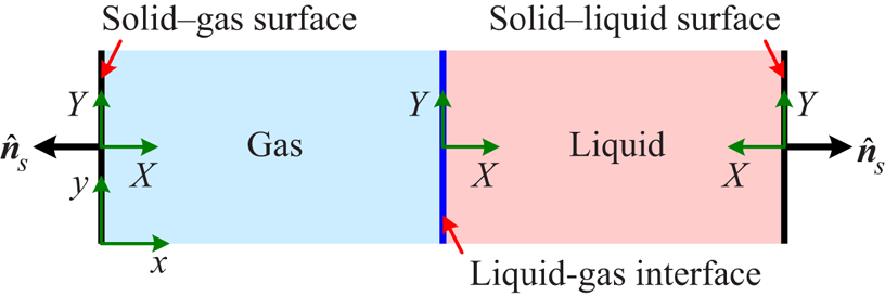
To theoretically determine the contact angle, we consider a one-dimensional multiphase system involving both solid–liquid and solid–gas surfaces, as shown by figure 1. Here, the solid–liquid surface means that the solid surface is immersed in the bulk liquid phase and the solid–gas surface means that the solid surface is immersed in the bulk gas phase. When the multiphase system is in an equilibrium state, the above introduced chemical potential should be spatially uniform, which means $\boldsymbol {\nabla } \boldsymbol {\cdot } \boldsymbol{\mathsf{P}} = \boldsymbol {0}$. Therefore, we have

(3.5)\begin{equation} P_0 \equiv P_{xx} = p_\textit{EOS} - \kappa \rho \frac{\mathrm{d}^2 \rho}{\mathrm{d}\kern0.06em x^2} + \frac{\kappa}{2} \left( \frac{\mathrm{d} \rho}{\mathrm{d}\kern0.06em x} \right)^2 = p_\textit{EOS} - \frac{\kappa}{2} \rho^2 \frac{\mathrm{d}}{\mathrm{d} \rho} \left[ \frac{1}{\rho} \left( \frac{\mathrm{d} \rho}{\mathrm{d}\kern0.06em x} \right)^2 \right] , \end{equation}

where $P_0$ is a constant pressure and $P_0 = p_\textit {EOS} (\rho _l ) = p_\textit {EOS} (\rho _g )$. Considering ${\mathrm {d} \rho }/{\mathrm {d} x} = 0$ in the bulk liquid and gas phases and then integrating equation (3.5) from $\rho _g$ to $\rho _l$ (i.e. from the bulk gas phase to the bulk liquid phase), we have

(3.6)\begin{equation} \int_{\rho_g }^{\rho_l } ( P_0 -p_\textit{EOS} ) \, \mathrm{d} v = 0, \end{equation}

where $v = \rho ^{-1}$ is the specific volume. In thermodynamic theory, (3.6) is known as the Maxwell construction, from which the liquid density $\rho _l$ and gas density $\rho _g$, as well as the pressure $P_0$, can be theoretically determined to arbitrary precision using numerical integration. The indefinite integral of (3.5) can be written as

(3.7)\begin{equation} \frac{\kappa}{2} \left( \frac{\mathrm{d} \rho}{\mathrm{d}\kern0.06em x} \right)^2 = \rho \left[ \int ( P_0 - p_\textit{EOS} ) \, \mathrm{d} v + C \right] , \end{equation}

where the integration constant $C$ can be determined by the condition ${\mathrm {d} \rho }/{\mathrm {d} x} = 0$ for $\rho = \rho _l$ or $\rho _g$ (i.e. ${\mathrm {d} \rho }/{\mathrm {d} x} = 0$ in the bulk liquid and gas phases). To simplify the notation, we introduce

(3.8)\begin{equation} {\varPhi} \equiv \sqrt{ \rho \left[ \int ( P_0 - p_\textit{EOS} ) \, \mathrm{d} v + C \right] } , \end{equation}

and then (3.7) can be rewritten as

(3.9)\begin{equation} \sqrt{ \frac{\kappa}{2} } \left| \frac{\mathrm{d} \rho}{ \mathrm{d}\kern0.06em x } \right| = {\varPhi} . \end{equation}

Note that ${\varPhi}$ is a function of $\rho$, which is completely determined by the multiphase EOS, and we should have ${\varPhi} \geq 0$ according to (3.8).

Figure 1.

Schematic of the one-dimensional multiphase system involving both solid–liquid and solid–gas surfaces, where $(x, y)$ denotes the global coordinate system and $(X, Y)$ denotes the local coordinate system with respect to the liquid–gas interface, solid–liquid surface or solid–gas surface.

Combining equations (3.4) and (3.9), on the solid surface we have

(3.10)\begin{equation} {\varPhi}( \rho_s ) = \frac{1}{ \sqrt{2 \kappa} } \left| \frac{\mathrm{\partial} \psi_s}{ \mathrm{\partial} \rho_s } \right| , \end{equation}

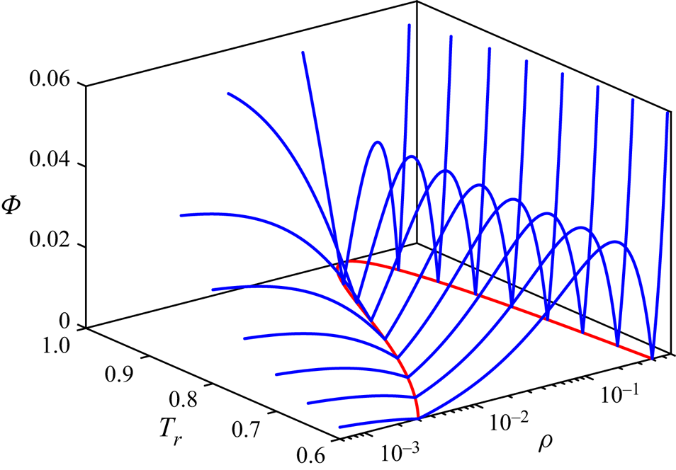
from which $\rho _s$ can be theoretically determined to arbitrary precision using a numerical technique. In the following, $\rho _s$ is denoted by $\rho _{sl}$ for the solid–liquid surface and $\rho _{sg}$ for the solid–gas surface, respectively. Figure 2 shows the curves for ${\varPhi}$ defined in (3.8) at various reduced temperatures, where the coexistence curve determined by the Maxwell construction is also plotted in the $\rho - T_r$ plane. As can be seen, ${\varPhi}$ decreases with $\rho$ in the range $\rho < \rho _g$, ${\varPhi}$ first increases and then decreases with $\rho$ in the range $\rho _g < \rho < \rho _l$, and ${\varPhi}$ increases with $\rho$ in the range $\rho > \rho _l$. For $\rho = \rho _g$ and $\rho _l$, ${\varPhi} = 0$. Since ${\varPhi}$ varies with $\rho$ non-monotonically in the vicinity of $\rho _l$ and ${\varPhi} (\rho _l ) = 0$, there could exist two possible solutions for $\rho _{sl}$ in (3.10), with one solution smaller than $\rho _l$ and the other larger than $\rho _l$ (see figure 3 as an example). If the fluid molecules have more favourable interactions with the solid molecules, it is expected that the fluid molecules will be concentrated on the solid surface and the solid surface behaves as hydrophilic. Therefore, the physically consistent solution for $\rho _{sl}$ can be determined by the principle that $\rho _{sl} > \rho _l$ for a hydrophilic surface and $\rho _{sl} < \rho _l$ for a hydrophobic surface. Similarly, there also exist two possible solutions for $\rho _{sg}$ in (3.10), and the physically consistent solution for $\rho _{sg}$ satisfies $\rho _{sg} > \rho _g$ for a hydrophilic surface and $\rho _{sg} < \rho _g$ for a hydrophobic surface.

Figure 2.

Curves for ${\varPhi}$ defined in (3.8) at various reduced temperatures, together with the coexistence curve determined by the Maxwell construction in the $\rho {-} T_r$ plane.

Figure 3.

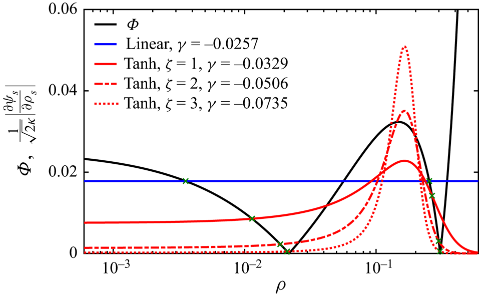
Determinations of the fluid densities on the solid surfaces by the intersections of the curves for ${\varPhi}$ and $({1}/{\sqrt {2 \kappa }}) | { \mathrm {\partial } \psi _s }/{ \mathrm {\partial } \rho _s } |$, where the conventional linear $\psi _s$ given in (3.15) and the present tanh $\psi _s$ with $\zeta = 1 {\sim} 3$ given in (3.16) are considered. The reduced temperature is set to $T_r = 0.8$ and the contact angle is fixed at $\theta = 140^\circ$, implying that $\rho _{sl} < \rho _l$ and $\rho _{sg} < \rho _g$.

The liquid–gas surface tension $\sigma _{lg}$ can be calculated as

(3.11)\begin{equation} \sigma_{lg} = \int_{gas}^{liquid} ( P_{XX} - P_{YY} ) \, \mathrm{d} X = \kappa \int_{\rho_g }^{\rho_l } \frac{\mathrm{d} \rho}{\mathrm{d} X}\, \mathrm{d} \rho = \sqrt{2 \kappa} \int_{\rho_g }^{\rho_l } {\varPhi} \mathrm{d} \rho , \end{equation}

where the integral from ‘gas’ to ‘liquid’ means an integral from the bulk gas phase to the bulk liquid phase. Note that ${\mathrm {d} \rho }/{\mathrm {d} X} > 0$ for the liquid–gas interface shown in figure 1. The solid–liquid surface tension $\sigma _{sl}$ can be calculated as

(3.12)\begin{align} \sigma_{sl} & = [ \psi_s (\rho_{sl} ) - \psi_s (0) ] + \int_{solid}^{liquid} ( P_{XX} - P_{YY} ) \, \mathrm{d} X = [ \psi_s (\rho_{sl} ) - \psi_s (0) ] + \kappa \int_{\rho_{sl} }^{\rho_l } \frac{\mathrm{d} \rho}{\mathrm{d} X}\, \mathrm{d} \rho \nonumber\\ & = [ \psi_s (\rho_{sl} ) - \psi_s (0) ] + \sqrt{2 \kappa} \int_{min (\rho_{sl} ,\rho_l )}^{max (\rho_{sl} , \rho_l )} {\varPhi} \mathrm{d} \rho , \end{align}

where the integral from ‘solid’ to ‘liquid’ means an integral from the solid–liquid surface to the bulk liquid phase. For the solid–liquid surface shown in figure 1, ${\mathrm {d} \rho }/{\mathrm {d} X} > 0$ if $\rho _{sl} < \rho _l$ or ${\mathrm {d} \rho }/{\mathrm {d} X} < 0$ if $\rho _{sl} > \rho _l$. Similarly, the solid–gas surface tension $\sigma _{sg}$ can be calculated as

(3.13)\begin{align} \sigma_{sg} & = [ \psi_s (\rho_{sg} ) - \psi_s (0) ] + \int_{solid}^{gas} ( P_{XX} - P_{YY} ) \, \mathrm{d} X = [ \psi_s (\rho_{sg} ) - \psi_s (0) ] + \kappa \int_{\rho_{sg} }^{\rho_g } \frac{\mathrm{d} \rho}{\mathrm{d} X}\, \mathrm{d} \rho \nonumber\\ & = [ \psi_s (\rho_{sg} ) - \psi_s (0) ] + \sqrt{2 \kappa} \int_{min (\rho_{sg} ,\rho_g )}^{max (\rho_{sg} , \rho_g )} {\varPhi} \mathrm{d} \rho , \end{align}

where the integral from ‘solid’ to ‘gas’ means an integral from the solid–gas surface to the bulk gas phase. For the solid–gas surface shown in figure 1, ${\mathrm {d} \rho }/{\mathrm {d} X} > 0$ if $\rho _{sg} < \rho _g$ or ${\mathrm {d} \rho }/{\mathrm {d} X} < 0$ if $\rho _{sg} > \rho _g$. It is worth pointing out that the above integrals in (3.11), (3.12) and (3.13) are performed in the corresponding local coordinate systems. The contact angle $\theta$ can then be calculated via Young's equation as follows:

(3.14)\begin{equation} \cos \theta = \frac{\sigma_{sg} - \sigma_{sl}}{ \sigma_{lg} } = \frac{ \displaystyle \frac{1}{\sqrt{2 \kappa}} [ \psi_s (\rho_{sg} ) - \psi_s (\rho_{sl} ) ] + \int_{min (\rho_{sg} ,\rho_g )}^{max (\rho_{sg} , \rho_g )} {\varPhi} \mathrm{d} \rho - \int_{min (\rho_{sl} ,\rho_l )}^{max (\rho_{sl} , \rho_l )} {\varPhi} \mathrm{d} \rho }{ \displaystyle \int_{\rho_g }^{\rho_l } {\varPhi} \mathrm{d} \rho } . \end{equation}

Note that the definite integral of ${\varPhi}$ with respect to $\rho$ in (3.14) can be theoretically determined to arbitrary precision using a numerical technique, and the contact angle $\theta$ denotes the static contact angle throughout this work unless otherwise stated.

Based on the above analysis, the contact angle can be unambiguously determined by the free-energy density for the solid surface once the multiphase EOS is specified in advance. Following Cahn (Reference Cahn1977), the free-energy density for the solid surface in linear form can be adopted

(3.15a)\begin{gather} \psi_s ={-} K_\textit{EOS} K_\textit{INT} \gamma \rho_s , \end{gather}

(3.15b)\begin{gather}\frac{\mathrm{\partial} \psi_s}{ \mathrm{\partial} \rho_s } ={-} K_\textit{EOS} K_\textit{INT} \gamma , \end{gather}

where the parameter $\gamma$ determines the contact angle $\theta$, and the scaling factors $K_\textit {EOS}$ and $K_\textit {INT}$ are introduced here to ensure that the contact angle, liquid–gas surface tension and liquid–gas interface thickness can be independently adjusted in the present theoretical framework. The above linear free-energy density has been widely adopted in the free-energy LB model in previous works (Briant et al. Reference Briant, Papatzacos and Yeomans2002, Reference Briant, Wagner and Yeomans2004; Semprebon et al. Reference Semprebon, Krüger and Kusumaatmaja2016; Krüger et al. Reference Krüger, Kusumaatmaja, Kuzmin, Shardt, Silva and Viggen2017). Figure 3 shows the determinations of the fluid densities on the solid surfaces by the intersections of the curves for ${\varPhi}$ and $({1}/{\sqrt {2 \kappa }}) | { \mathrm {\partial } \psi _s }/{ \mathrm {\partial } \rho _s } |$ according to (3.10) when $T_r = 0.8$ and $\theta = 140 ^\circ$. It can be seen that, for the linear free-energy density, $\rho _{sl}$ and $\rho _{sg}$ significantly deviate from $\rho _l$ and $\rho _g$, respectively, since the steepness of the curve for ${\varPhi}$ is relatively small for $T_r = 0.8$. Note that the significant deviation between the fluid densities on the solid surface and in the bulk phase is clearly in contradiction to physical reality although $\nabla _\perp \rho$ on the solid surface is non-zero because of the imbalance between the microscopic solid–fluid and fluid–fluid molecular interactions (see (3.4)). In fact, the linear $\psi _s$ was originally proposed for the wetting phenomenon near the critical point (Cahn Reference Cahn1977; de Gennes Reference de Gennes1985), implying that it could be inadequate when the reduced temperature is relatively low, such as $T_r = 0.8$ here. To remedy this defect, we propose a new free-energy density for the solid surface, which is in hyperbolic tangent (tanh) form, as follows:

(3.16a)\begin{gather} \psi_s ={-} K_\textit{EOS} K_\textit{INT} \frac{\gamma (\rho_l - \rho_g )}{2 \zeta} \tanh \left( \zeta \frac{2 \rho_s - \rho_l - \rho_g }{\rho_l - \rho_g } \right) , \end{gather}

(3.16b)\begin{gather}\frac{\mathrm{\partial} \psi_s}{ \mathrm{\partial} \rho_s } ={-} K_\textit{EOS} K_\textit{INT} \gamma \,\text{sech}^2 \left( \zeta \frac{2 \rho_s - \rho_l - \rho_g }{ \rho_l - \rho_g } \right) , \end{gather}

where the independent parameters $\zeta$ and $\gamma$ determine the contact angle $\theta$, and the scaling factors $K_\textit {EOS}$ and $K_\textit {INT}$ are introduced to ensure that $\theta$, $\sigma _{lg}$ and $W_{lg}$ can be independently adjusted in the present theoretical framework. Figure 3 also shows the curve for $({1}/{\sqrt {2 \kappa }}) | { \mathrm {\partial } \psi _s }/{ \mathrm {\partial } \rho _s } |$ for the present tanh free-energy density with $\zeta = 1$, $2$ and $3$. The contact angle is fixed at $\theta = 140^\circ$ by adjusting $\gamma$. It can be seen from figure 3 that $\rho _{sl}$ and $\rho _{sg}$ rapidly tend to $\rho _l$ and $\rho _g$, respectively, as $\zeta$ increases, which means that the deviation between the fluid densities on the solid surface and in the bulk phase can be dramatically reduced by increasing $\zeta$. Here, it is interesting to note that, when $\zeta \rightarrow 0$, the present tanh $\psi _s$ given in (3.16) can degenerate into the conventional linear $\psi _s$ given in (3.15).

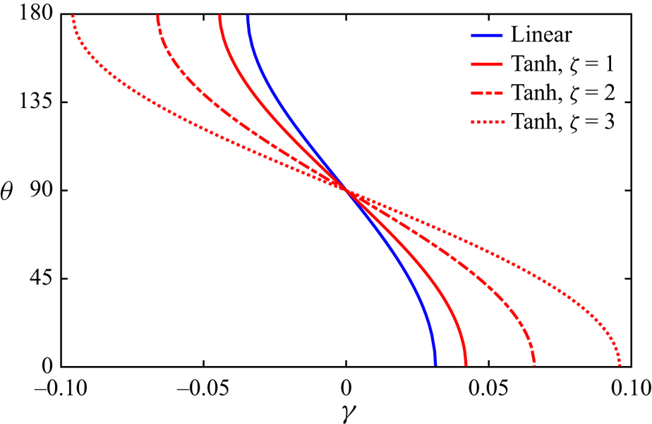
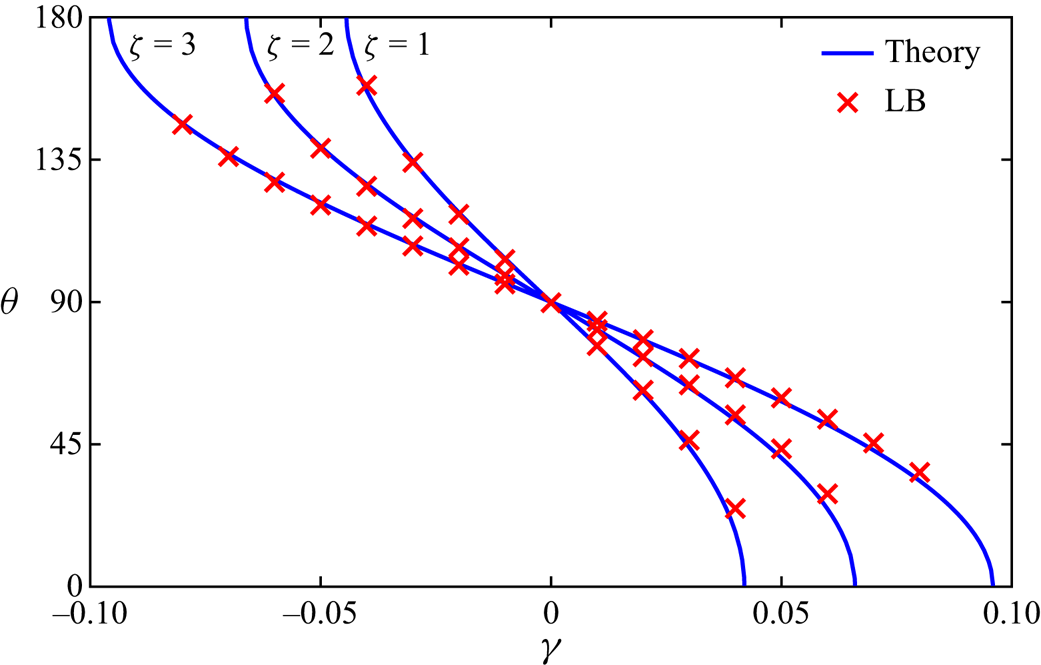
Figure 4 shows the dependences of the contact angle $\theta$, theoretically calculated by (3.14), on the parameter $\gamma$ for the conventional linear $\psi _s$ given in (3.15) and the present tanh $\psi _s$ with $\zeta = 1 {\sim} 3$ given in (3.16). It can be seen from figure 4 that the contact angle $\theta$ can be effectively adjusted from $0^\circ$ to $180^\circ$ by the parameter $\gamma$ for both the conventional linear and present tanh $\psi _s$. 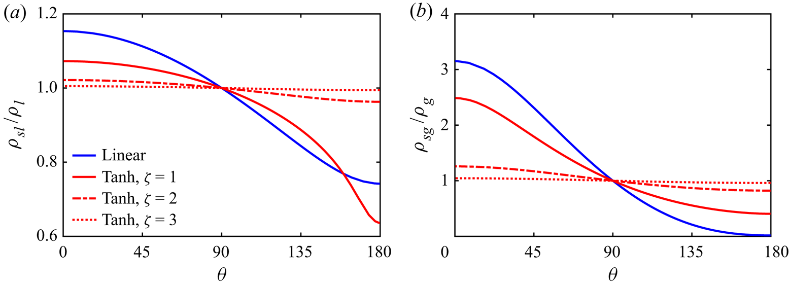Meanwhile, the curves for $\theta$ obtained by these different $\psi _s$ are similar to each other, and the steepness of the curve for $\theta$ tends to infinity when $\theta \rightarrow 0^\circ$ or $180^\circ$. Figure 5 shows the variations of the fluid densities on the solid–liquid and solid–gas surfaces, which are normalized by the densities in the bulk liquid and gas phases, respectively, with the contact angle for the conventional linear and present tanh $\psi _s$. As can be seen, both $\rho _{sl} / \rho _l$ and $\rho _{sg} / \rho _g$ deviate from $1$ as long as $\theta \neq 90^\circ$, and the deviation becomes larger as $| \theta - 90^\circ |$ increases. Meanwhile, both $\rho _{sl} / \rho _l$ and $\rho _{sg} / \rho _g$ are quite close to $1$ for the present tanh $\psi _s$ with $\zeta = 3$ and even $2$, implying that the deviation between the fluid densities on the solid surface and in the bulk phase are dramatically reduced. To be quantitative, $\rho _{sl} / \rho _l$ and $\rho _{sg} / \rho _g$ are in the ranges $[0.994213 , 1.004987]$ and $[0.959740 , 1.044475]$, respectively, for the tanh $\psi _s$ with $\zeta = 3$, and they are in the ranges $[0.962851 , 1.021547]$ and $[0.821519 , 1.258193]$, respectively, for the tanh $\psi _s$ with $\zeta = 2$. On the contrary, $\rho _{sl} / \rho _l$ and $\rho _{sg} / \rho _g$ are in the ranges $[0.636389 , 1.072573]$ and $[0.405167 , 2.486218]$, respectively, for the tanh $\psi _s$ with $\zeta = 1$ and in the ranges $[0.742080 , 1.153527]$ and $[0.015796 , 3.151205]$, respectively, for the linear $\psi _s$. To demonstrate that the contact angle $\theta$ can be adjusted independently of the liquid–gas surface tension $\sigma _{lg}$ and liquid–gas interface thickness $W_{lg}$, the theoretical calculations are repeated here with different $\sigma _{lg}$ ($0.01$ and $0.02$) and $W_{lg}$ ($10$ and $15$). 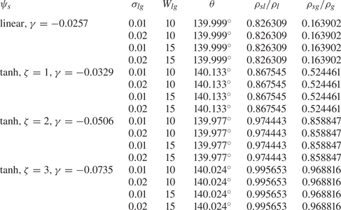Without loss of generality and following the results in figure 3, the parameter $\gamma$ is set to $-0.0257$ for the conventional linear $\psi _s$, and it is set to $-0.0329$, $-0.0506$ and $-0.0735$ for the present tanh $\psi _s$ with $\zeta = 1$, $2$ and $3$, respectively. The theoretical results are given in table 1. As can be seen, the contact angle $\theta$, as well as the normalized fluid density on the solid–liquid surface $\rho _{sl} / \rho _l$ and the normalized fluid density on the solid–gas surface $\rho _{sg} / \rho _g$, does indeed remain unchanged when $\sigma _{lg}$ and $W_{lg}$ are adjusted, as long as the parameter $\gamma$ is fixed for both the conventional linear and present tanh $\psi _s$. Therefore, $\theta$, $\sigma _{lg}$ and $W_{lg}$ can be independently adjusted via the parameter $\gamma$ and the scaling factors $K_\textit {EOS}$ and $K_\textit {INT}$ in the present theoretical framework. Before proceeding further, it is worth pointing out a temperature-dependent contact angle can be straightforwardly achieved in the present theoretical framework since the contact angle can be freely specified. The only point is to repeat the above theoretical calculation to get the dependence of the contact angle $\theta$ on the parameter $\gamma$ at various reduced temperatures.

Figure 4.

Dependences of the contact angle $\theta$ on the parameter $\gamma$ for the conventional linear $\psi _s$ given in (3.15) and the present tanh $\psi _s$ with $\zeta = 1 {\sim} 3$ given in (3.16).

Figure 5.

Variations of (a) the normalized fluid density on the solid–liquid surface $\rho _{sl} / \rho _l$ and (b) the normalized fluid density on the solid–gas surface $\rho _{sg} / \rho _g$ with the contact angle $\theta$ for the conventional linear $\psi _s$ given in (3.15) and the present tanh $\psi _s$ with $\zeta = 1 {\sim} 3$ given in (3.16).

Table 1.

Contact angle $\theta$, normalized fluid density on the solid–liquid surface $\rho _{sl} / \rho _l$ and normalized fluid density on the solid–gas surface $\rho _{sg} / \rho _g$ theoretically calculated with different liquid–gas surface tensions $\sigma _{lg}$ ($0.01$ and $0.02$) and liquid–gas interface thicknesses $W_{lg}$ ($10$ and $15$) for the conventional linear $\psi _s$ given in (3.15) and the present tanh $\psi _s$ with $\zeta = 1 {\sim} 3$ given in (3.16).

4. Wetting condition

Based on the surface thermodynamics analysed in § 3, a thermodynamically consistent treatment for the wetting condition can then be proposed for the recent multiphase LB model with a self-tuning EOS since the model itself is strictly consistent with thermodynamic theory. The no-slip condition on the solid surface can be handled by the improved non-equilibrium-extrapolation scheme proposed by Huang, Wu & Adams (Reference Huang, Wu and Adams2019b), where the distribution function is decomposed into three parts rather than two. In this scheme, the density on the wall node is locally determined through an auxiliary bounce-back process and the local conservation of mass can be strictly satisfied. Therefore, the key point in treating the wetting condition is to calculate the pairwise interaction force on the wall node. After the force on the wall node is obtained, the density distribution functions are reconstructed through the improved non-equilibrium-extrapolation scheme to realize the no-slip condition (Huang et al. Reference Huang, Wu and Adams2019b).

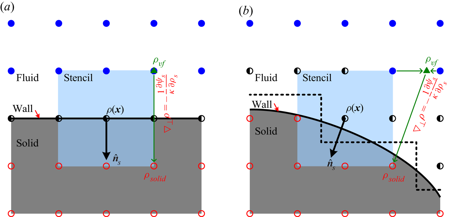
In the present wetting condition treatment, the pairwise interaction force on the wall node is normally calculated via (2.3), where the densities on the fluid and wall nodes in the nearest-neighbour interaction stencil are already known considering the no-slip condition treatment and the density on the solid node in the interaction stencil can be evaluated based on (3.4) (i.e. $\nabla _\perp \rho = - ({1}/{\kappa }) {\mathrm {\partial } \psi _s}/{\mathrm {\partial } \rho _s }$). For this purpose, a virtual fluid point $\boldsymbol {x}_\textit {vf}$ is first set along the inward normal direction (i.e. $- \hat {\boldsymbol {n}}_s$) as

(4.1)\begin{equation} \boldsymbol{x}_\textit{vf} = \boldsymbol{x}_{solid} - \frac{2 \delta_x}{ max (|\hat{n}_{s,x}| , |\hat{n}_{s,y}|) } \hat{\boldsymbol{n}}_s , \end{equation}

where $\boldsymbol {x}_{solid}$ denotes the solid node in the interaction stencil and $max (|\hat {n}_{s,x}| , |\hat {n}_{s,y}|)$ is introduced to ensure that $\boldsymbol {x}_\textit {vf}$ lies on a grid line, as illustrated in figure 6. For the straight wall shown in figure 6(a), $max (|\hat {n}_{s,x}| , |\hat {n}_{s,y}|) = 1$, and the virtual fluid point overlaps with one fluid node. Thus, the density on the virtual fluid point, denoted by $\rho _\textit {vf}$, can be directly obtained. As for the curved wall shown in figure 6(b), ${\sqrt {2}}/{2} \leq max (|\hat {n}_{s,x}| , |\hat {n}_{s,y}|) \leq 1$, and the virtual fluid point lies between two fluid and/or wall nodes on which the densities are known. Therefore, a linear interpolation can be employed to obtain $\rho _\textit {vf}$. Once the density on the virtual fluid point is obtained, the density on the solid node in the nearest-neighbour interaction stencil can be evaluated based on (3.4) as follows:

(4.2)\begin{equation} \rho_{solid} = \rho_\textit{vf} - \frac{2 \delta_x}{ max (|\hat{n}_{s,x}| , |\hat{n}_{s,y}|)} \frac{1}{\kappa} \frac{\mathrm{\partial} \psi_s}{\mathrm{\partial} \rho_s } . \end{equation}

Note that there could have more than one solid node in the interaction stencil, as illustrated in figure 6, and the density on each solid node should be individually evaluated through the above procedures. Moreover, for the present tanh $\psi _s$ given in (3.16), the fluid density on the solid surface $\rho _s$ is involved in the term ${\mathrm {\partial } \psi _s}/{\mathrm {\partial } \rho _s }$ on the right-hand side of (4.2). In real applications, $\rho _s$ in ${\mathrm {\partial } \psi _s}/{\mathrm {\partial } \rho _s }$ on the right-hand side of (4.2) is approximated by the following average density:

(4.3)\begin{equation} \rho_\textit{ave} = \frac{\displaystyle \sum_{i=0}^{N-1} s (\boldsymbol{x} + \boldsymbol{e}_i \delta_t) \rho (\boldsymbol{x} + \boldsymbol{e}_i \delta_t)}{\displaystyle \sum_{i=0}^{N-1} s (\boldsymbol{x} + \boldsymbol{e}_i \delta_t)} , \end{equation}

which shows better performance based on our numerical tests. Here, $s (\boldsymbol {x} + \boldsymbol {e}_i \delta _t)$ is a switch function that equals $1$ for the fluid and wall nodes and $0$ for the solid node. From the above analysis, it can be seen that the contact angle is not directly involved in the wetting condition treatment, and only the free-energy density for the solid surface that recovers the targeted contact angle is prescribed. The dynamic contact angle at the moving contact line is part of the solution obtained by the present LB model, and thus it is free to be the other value, suggesting that the so-called microscopic contact angle, widely assumed in theoretical analyses as the boundary condition, need not be introduced in the present framework.

Figure 6.

Schematic of the wetting condition treatment for (a) a straight wall and (b) a curved wall, where $\hat {\boldsymbol {n}}_s$ is the outward unit normal vector of the solid surface, $\rho _\textit {vf}$ is the density on the virtual fluid point denoted by the symbol ‘$\blacktriangle$ (green)’ and the symbols ‘$\bullet$ (blue)’, ‘$\circ$ (black)’ and ‘$\circ$ (red)’ denote the fluid, wall and solid nodes, respectively.

5. Validations and discussions

In this section, numerical tests are performed to validate the theoretical analysis of the surface thermodynamics in § 3 and the thermodynamically consistent treatment for the wetting condition in § 4. In the simulations, the present new free-energy density for the solid surface (i.e. the tanh $\psi _s$ given in (3.16)) is adopted. The additional cubic terms of velocity are eliminated by the modifications in Appendix A, and the basic parameters are given in § 2. The relaxation parameters in $\boldsymbol{\mathsf{S}}$ are set as $s_0 = s_j = 1$, $s_p = \tau _f^{-1}$ and $s_\varepsilon = s_p$, and also under the constraint of (2.12). Here, $\tau _f$ is the dimensionless relaxation time, which is set to $1.5$ unless otherwise stated.

5.1. Droplet on straight wall

A static droplet on a straight wall is first simulated on a $1024 \delta _x \times 512 \delta _x$ domain. The solid wall is put on the lower side of the domain, a mirror boundary condition is imposed on the upper side and periodic boundary conditions are applied in the $x$ direction. Initially, the density and velocity fields are set to

(5.1a)\begin{gather} \rho (\boldsymbol{x}, 0) = \frac{\rho_l + \rho_g }{2} - \frac{\rho_l - \rho_g }{2} \tanh \frac{ |\boldsymbol{x} - \boldsymbol{x}_c| - R_0 }{ W_{lg} / \ln (19) } , \end{gather}

(5.1b)\begin{gather}\boldsymbol{u} (\boldsymbol{x}, 0) = \boldsymbol{0} , \end{gather}

where $\boldsymbol {x}_c = (512\delta _x , 0)^\mathrm {T}$ and $R_0$ is chosen as $256 \delta _x$ and $128 \delta _x$ for the hydrophobic and hydrophilic surfaces, respectively. Then, the simulation is run to a steady state, and a static droplet on a straight wall can be obtained. Note that the liquid–gas interface thickness is defined from $\rho = 0.95 \rho _g + 0.05 \rho _l$ to $0.05 \rho _g + 0.95 \rho _l$ and the liquid–gas interface position is defined at $\rho = 0.5 \rho _g + 0.5 \rho _l$ throughout this work.

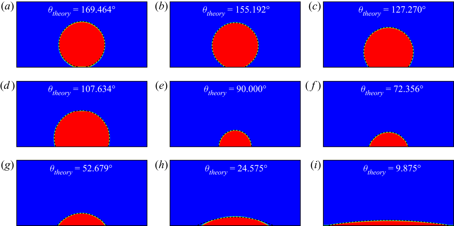
Figure 7 shows the droplets in the final steady state simulated with $\zeta = 2$ and $\gamma$ varying from $-0.065$ to $0.065$. As can be seen, the parameter $\gamma$ in the present tanh $\psi _s$ can effectively adjust the contact angle and the present wetting condition treatment can achieve a contact angle from superhydrophobic ($\theta > 150^\circ$) to superhydrophilic ($\theta < 30^\circ$). Moreover, the droplet profile obtained by the LB simulation agrees well with the analytical profile, which is determined by the contact angle derived from thermodynamic theory (see (3.14)) and the droplet volume conservation. This good agreement validates both the theoretical analysis of the surface thermodynamics in § 3 and the thermodynamically consistent treatment for the wetting condition in § 4. It is worth noting that there exists a low-density layer above the solid–liquid surface (i.e. below the droplet) for $\gamma = -0.065$ ($\theta _\textit {theory} = 169.464^\circ$), resulting in the contact angle obtained by the LB simulation being obviously smaller than the theoretical one (see figure 7a). Similarly, there exists a high-density layer above the solid–gas surface for $\gamma = 0.065$ ($\theta _\textit {theory} = 9.875^\circ$), which tends to make the droplet spread further on the solid surface. Since the simulation domain is finite and also periodic in the $x$ direction, the left and right three-phase contact points encounter each other (see figure 7i) and thus the droplet will eventually evolve into a liquid layer covering the solid surface in the present simulation.

Figure 7.

Static droplets on a straight wall for $\zeta = 2$ and (a) $\gamma = - 0.065$, (b) $\gamma = - 0.060$, (c) $\gamma = - 0.040$, (d) $\gamma = - 0.020$, (e) $\gamma = 0.000$, (f) $\gamma = 0.020$, (g) $\gamma = 0.040$, (h) $\gamma = 0.060$, (i) $\gamma = 0.065$, where $\theta _\textit {theory}$ is the contact angle predicted by thermodynamic theory and the dashed line denotes the analytical droplet profile determined by $\theta _\textit {theory}$ and droplet volume conservation.

For quantitative comparison, the static contact angle is numerically measured by fitting the liquid–gas interface with a circular segment. Figure 8 compares the contact angle obtained by the LB simulation with that predicted by thermodynamic theory (i.e. (3.14)). In the simulations, the parameter $\gamma$ is set in the range $[-0.04 , 0.04]$, $[-0.06 , 0.06]$ and $[-0.08 , 0.08]$ for $\zeta = 1$, $2$ and $3$, respectively. 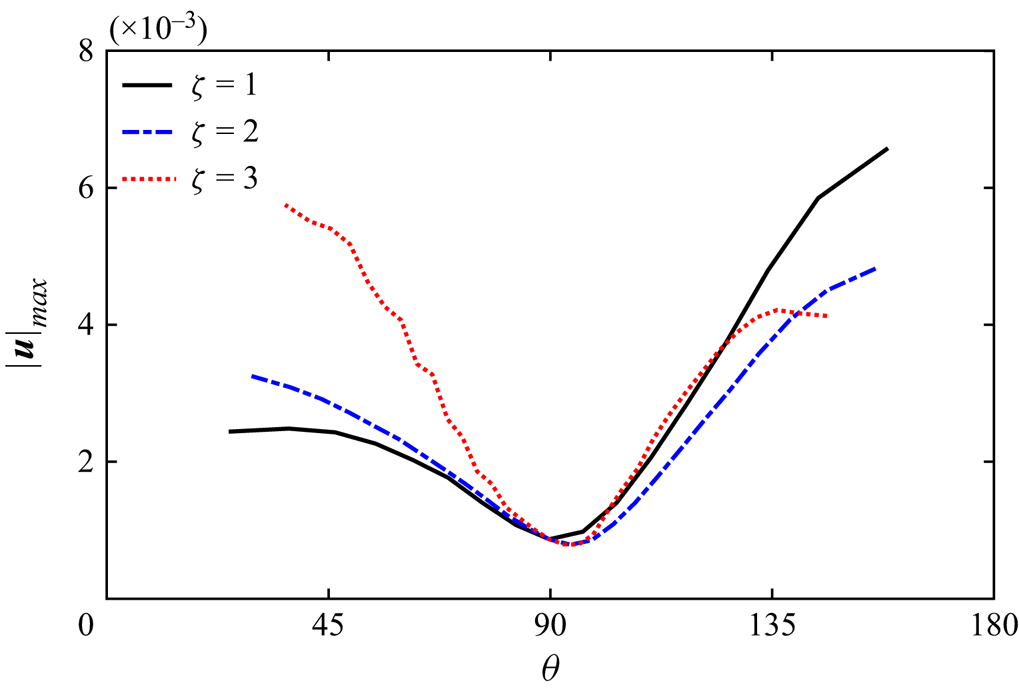It can be seen from figure 8 that $\theta$ by the LB simulation is in good agreement with the theoretical value, which confirms the theoretical analysis of the surface thermodynamics in § 3 and the thermodynamically consistent treatment for the wetting condition in § 4. Figure 9 shows the corresponding maximum magnitude of the spurious velocity (denoted by $|\boldsymbol {u}_{max}|$) in the LB simulation. As can be seen, $|\boldsymbol {u}_\textit {max}|$ approximately decreases with $\theta$ in the range $\theta < 90^\circ$ (i.e. for the hydrophilic surface) and increases with $\theta$ in the range $\theta > 90^\circ$ (i.e. for the hydrophobic surface). Moreover, $|\boldsymbol {u}|_\textit {max}$ with $\zeta = 3$ is obviously larger than $|\boldsymbol {u}|_\textit {max}$ with $\zeta = 1$ and $2$ when $\theta < 90^\circ$, while $|\boldsymbol {u}|_\textit {max}$ with $\zeta = 2$ is slightly smaller than $|\boldsymbol {u}|_\textit {max}$ with $\zeta = 1$ and $3$ when $\theta > 90 ^\circ$. It is worth pointing out that $|\boldsymbol {u}|_\textit {max}$ with $\zeta = 3$ remains at the same level when $\theta > 130^\circ$ and thus it becomes the smallest one when $\theta > 140^\circ$. 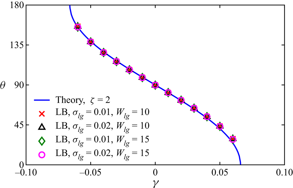However, as the contact angle increases, the simulation with $\zeta = 3$ suffers from the defect of the low-density layer (see figure 7a) earlier than the simulations with $\zeta = 1$ and $2$. Finally, the simulations are also repeated here with different liquid–gas surface tensions $\sigma _{lg}$ ($0.01$ and $0.02$) and liquid–gas interface thicknesses $W_{lg}$ ($10$ and $15$) to numerically demonstrate that $\theta$, $\sigma _{lg}$ and $W_{lg}$ can be independently adjusted in the present theoretical framework. The parameter $\zeta$ in the tanh $\psi _s$ is chosen as $2$ without loss of generality, and the parameter $\gamma$ is set in the range $[-0.06 , 0.06]$. Figure 10 shows the static contact angles measured by circular fitting to the liquid–gas interface. As can be seen, there is no distinguishable difference between $\theta$ numerically obtained with different $\sigma _{lg}$ and $W_{lg}$, suggesting that $\theta$, $\sigma _{lg}$ and $W_{lg}$ can be independently adjusted in real applications.

Figure 8.

Comparison of the contact angle obtained by the LB simulation of a static droplet on a straight wall with that predicted by thermodynamic theory for $\zeta = 1$, $2$ and $3$.

Figure 9.

Maximum magnitudes of the spurious velocity in the LB simulation of a static droplet on a straight wall for $\zeta = 1$, $2$ and $3$.

Figure 10.

Contact angles numerically obtained with different liquid–gas surface tensions $\sigma _{lg}$ ($0.01$ and $0.02$) and liquid–gas interface thicknesses $W_{lg}$ ($10$ and $15$) in the LB simulation of a static droplet on a straight wall.

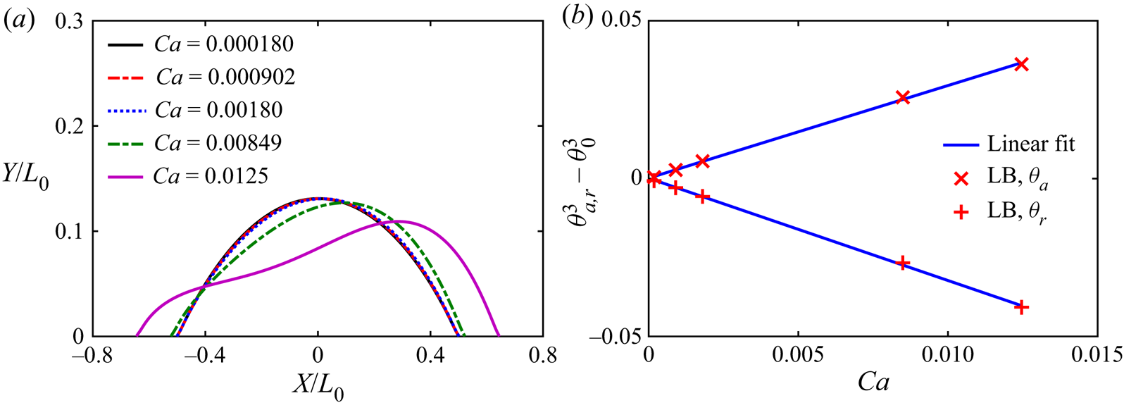
The above validations concern a static droplet on a straight wall, and in the following, a sliding droplet on a straight wall is simulated to study the dynamic performance of the present wetting condition treatment. For this purpose, after the static droplet is obtained, an external force parallel to the $x$ direction is applied and then the droplet starts sliding on the wall. The parameters $\zeta$ and $\gamma$ in the tanh $\psi _s$ are chosen as $2$ and $0.060$, respectively, and the corresponding static droplet is shown in figure 7(h). The profiles of the sliding droplet are shown in figure 11(a) for various capillary numbers, defined as $C\mspace {-1.5mu}a = \mu _l U / \sigma _{lg}$ with $\mu _l$ the dynamic viscosity of the liquid phase and $U$ the moving velocity of the three-phase contact point. Note that the local coordinate system $(X, Y)$ is fixed at the middle point of the droplet, and the coordinates are scaled with $L_0$, the length of the corresponding static droplet. It can be seen that the sliding droplet is more obviously stretched as $C\mspace {-1.5mu}a$ increases, and the dynamic advancing contact angle $\theta _a$ and dynamic receding contact angle $\theta _r$ are slightly larger and smaller than the static contact angle $\theta _0$, respectively. For quantitative comparison, $\theta _a$ and $\theta _r$ (in radians) are numerically measured and then validated with the Cox–Voinov law (Voinov Reference Voinov1976; Cox Reference Cox1986)

(5.2)\begin{equation} \theta_{a,r}^3 = \theta_0^3 \pm 9 C\mspace{-1.5mu}a \ln \left( \frac{h_\theta}{\ell_s} \right) , \end{equation}

where ‘$+$’ and ‘$-$’ are for the advancing and receding contact lines, respectively, $\ell _s$ is the microscopic slip length used to remove the viscous singularity at the moving contact line (Hocking Reference Hocking1983) and $h_\theta$ denotes a macroscopic position where the dynamic contact angle is measured. It should be emphasized that (5.2) is derived in the context of the sharp interface representation and constant microscopic contact angle. However, the liquid–gas interface in the present multiphase LB model is diffuse rather than sharp, implying that the microscopic slip condition is not required (Sbragaglia, Sugiyama & Biferale Reference Sbragaglia, Sugiyama and Biferale2008). Meanwhile, the free-energy density for the solid surface, rather than the contact angle, is prescribed for the present wetting condition treatment, and thus the hypothesis of constant microscopic contact angle is also not required. Nevertheless, we can measure $\theta _a$ and $\theta _r$ at the wall in the LB simulation and then set $h_\theta = \delta _x$ to facilitate the validation with the Cox–Voinov law. Figure 11(b) shows the variations of the cubes of $\theta _a$ and $\theta _r$ with $C\mspace {-1.5mu}a$. As seen, both $\theta _a^3$ and $\theta _r^3$ vary linearly with $C\mspace {-1.5mu}a$ and $\theta _a + \theta _r \approx 2 \theta _0$ in the small $C\mspace {-1.5mu}a$ range. An equivalent microscopic slip length for the present wetting condition treatment can then be evaluated via (5.2), which is $0.722 \delta _x$ and $0.698 \delta _x$ for the advancing and receding contact lines, respectively. Therefore, the microscopic and macroscopic lengths can be well separated in the present LB simulations.

Figure 11.

(a) Profiles of sliding droplets on a straight wall at various capillary numbers $C\mspace {-1.5mu}a$. (b) Variations of the cubes of the dynamic advancing contact angle $\theta _a$ and dynamic receding contact angle $\theta _r$ (in radians) with the capillary number $C\mspace {-1.5mu}a$, where $\theta _0$ is the static contact angle numerically measured at $C\mspace {-1.5mu}a = 0$.

5.2. Droplet on curved wall

To further validate the present wetting condition treatment, a static droplet on a curved wall is simulated on a $1024 \delta _x \times 1024 \delta _x$ domain with periodic boundary conditions in both the $x$ and $y$ directions. A solid circular cylinder of radius $256 \delta _x$ and centre $(512 \delta _x , 384 \delta _x)^\mathrm {T}$ is placed in the domain. The density and velocity fields are initialized as

(5.3a)\begin{gather} \rho (\boldsymbol{x}, 0) = \frac{\rho_l + \rho_g }{2} - \frac{\rho_l - \rho_g }{2} \tanh \frac{ |\boldsymbol{x} - \boldsymbol{x}_c| - R_0 }{ W_{lg} / \ln (19) } , \end{gather}

(5.3b)\begin{gather}\boldsymbol{u} (\boldsymbol{x}, 0) = \boldsymbol{0} , \end{gather}

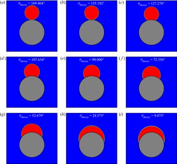
where $\boldsymbol {x}_c = (512\delta _x , 640\delta _x)^\mathrm {T}$ and $R_0 = 192 \delta _x$. The droplets in the final steady state, which are simulated with $\zeta = 2$ and $\gamma$ varying from $-0.065$ to $0.065$, are shown in figure 12, where the analytical density profiles determined by the theoretical contact angle and droplet volume conservation are also plotted. Good agreement between the droplets by the LB simulations and the analytical profiles can be observed, which demonstrates the applicability and accuracy of the present thermodynamically consistent treatment for the wetting condition for a curved wall. For $\gamma = -0.065$ ($\theta _\textit {theory} = 169.464^\circ$), there exists a low-density layer below the droplet on a curved wall, which is similar to the droplet on a straight wall (see figure 7a). As for $\gamma = 0.065$ ($\theta _\textit {theory} = 9.875^\circ$), a static droplet can be obtained for the curved wall in the present simulation, which is different from the droplet on a straight wall (see figure 7i) that eventually evolves into a liquid layer covering the solid surface. Such a difference between the droplets on straight and curved walls for $\gamma = 0.065$ can be explained as follows: the curved wall in the LB simulation is stepwise rather than ideally smooth (see figure 6(b) as an example), and thus the three-phase contact point could be pinned at the corner, implying that the spread of the droplet on the curved wall is terminated and the formation of the high-density layer above the solid–gas surface is prevented. Meanwhile, the pinning of the contact point at the corner makes the apparent contact angle shown in figure 12(i) significantly larger than the theoretical one calculated via Young's equation.

Figure 12.

Static droplets on a curved wall for $\zeta = 2$ and (a) $\gamma = - 0.065$, (b) $\gamma = - 0.060$, (c) $\gamma = - 0.040$, (d) $\gamma = - 0.020$, (e) $\gamma = 0.000$, (f) $\gamma = 0.020$, (g) $\gamma = 0.040$, (h) $\gamma = 0.060$, (i) $\gamma = 0.065$, where $\theta _\textit {theory}$ is the contact angle predicted by thermodynamic theory and the dashed line denotes the analytical droplet profile determined by $\theta _\textit {theory}$ and droplet volume conservation.

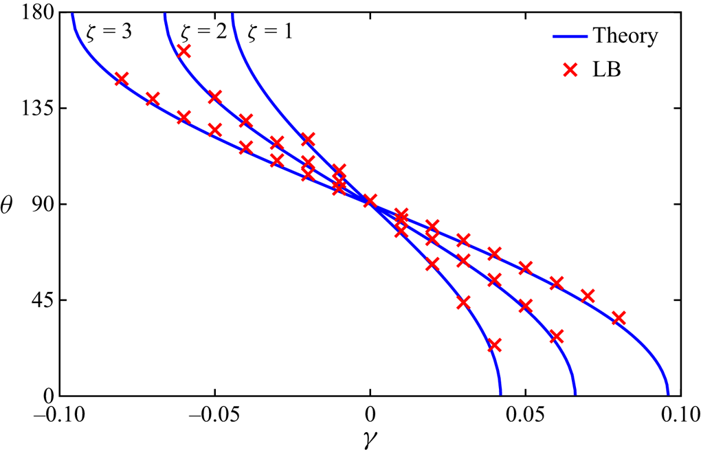
The static contact angle in the LB simulation is measured by fitting the liquid–gas interface with a circular segment and is then compared with that predicted by thermodynamic theory in figure 13. In the simulations, the parameter $\gamma$ in the tanh $\psi _s$ is set in the range $[-0.04 , 0.04]$, $[-0.06 , 0.06]$ and $[-0.08 , 0.08]$ for $\zeta = 1$, $2$ and $3$, respectively. 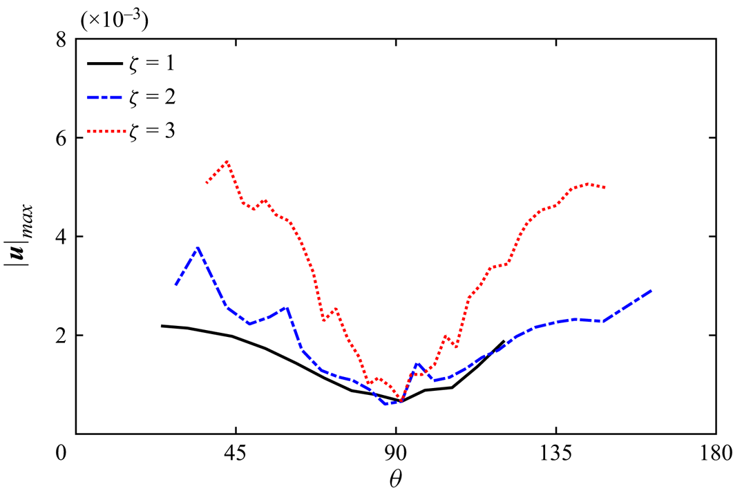Note that the simulation with $\zeta = 1$ blows up when $\gamma \leq -0.025$, which could be caused by the no-slip condition treatment for a curved wall and deserves further specific investigation. As can be seen from figure 13, the contact angle by the LB simulation corresponds well with the prediction by thermodynamic theory as long as the simulation is numerically stable, which reconfirms the theoretical analysis of the surface thermodynamics in § 3 and the thermodynamically consistent treatment for the wetting condition in § 4. Figure 14 shows the variation of the maximum magnitude of the spurious velocity $| \boldsymbol {u} |_\textit {max}$ with the contact angle $\theta$ in the LB simulation. It can be seen that $| \boldsymbol {u} |_\textit {max}$ with $\zeta = 3$ is obviously larger than $| \boldsymbol {u} |_\textit {max}$ with $\zeta = 1$ and $2$ for both $\theta < 90^\circ$ and $\theta > 90^\circ$. In the range $\theta < 70^\circ$, $| \boldsymbol {u} |_\textit {max}$ with $\zeta = 1$ is smaller than $| \boldsymbol {u} | _\textit {max}$ with $\zeta = 2$, while in the range $70^\circ < \theta < 120 ^\circ$, $|\boldsymbol {u}|_\textit {max}$ with $\zeta = 1$ and $2$ are quite close to each other. In the range $\theta > 120^\circ$ that corresponds to $\gamma \leq -0.025$ for $\zeta = 1$, the simulation with $\zeta = 1$ blows up. Comparing figure 14 with figure 9, it can be found that the maximum magnitude of the spurious velocity remains at the same level for the static droplets on curved and straight walls. Meanwhile, the curve of $| \boldsymbol {u} |_\textit {max}$ vs $\theta$ becomes relatively bumpy as $\zeta$ increases, which can be explained as follows: the maximum magnitude of the spurious velocity is observed close to the three-phase contact point, and the bumpy behaviour is caused by the relative position of the liquid–gas interface with respect to the lattice nodes, which is disordered in the simulations. As $\zeta$ increases, the contribution to the wetting condition is more concentrated (see figure 3) and thus the bumpy behaviour becomes more sensitive to the relative position of the phase interface. Nevertheless, considering that the spurious velocity is a numerical defect caused by many subtle factors, a very neat trend of its maximum magnitude vs the contact angle is not expected.

Figure 13.

Comparison of the contact angle obtained by the LB simulation of a static droplet on a curved wall with that predicted by thermodynamic theory for $\zeta = 1$, $2$ and $3$.

Figure 14.

Maximum magnitudes of the spurious velocity in the LB simulation of a static droplet on a curved wall for $\zeta = 1$, $2$ and $3$.

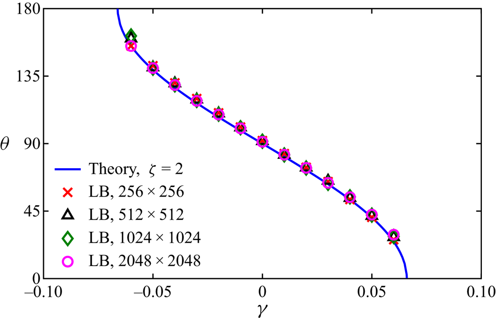
Before closing this section, a grid-independence study of the present simulation is performed. The grid size $N_x \times N_y$ is set to $256 \times 256$, $512 \times 512$, $1024 \times 1024$ and $2048 \times 2048$ and the liquid–gas interface thickness $W_{lg}$ is fixed at $10$. The radius and centre of the solid circular cylinder, as well as $\boldsymbol {x}_c$ and $R_0$ in (5.3), are proportionally adjusted as the grid size varies. The parameter $\zeta$ in the tanh $\psi _s$ is chosen as $2$, and the parameter $\gamma$ is set in the range $[-0.06 , 0.06]$. As shown by figure 15, the contact angles numerically obtained with different grid sizes agree well with each other and are also in good agreement with the theoretical result. It is worth noting that the curved wall is represented as a stepwise shape in the simulation, and thus the grid refinement cannot alleviate the pinning of the contact point at the corner. Moreover, for the grid size $256 \times 256$, the droplet on the circular cylinder degenerates into a droplet on a locally straight wall when the contact angle is large enough (such as $\gamma = 0.060$) because the radii of the droplet and circular cylinder are too small. Therefore, a higher accuracy on the contact angle is observed when $\gamma = 0.060$ for $N_x \times N_y = 256 \times 256$.

Figure 15.

Contact angles numerically obtained with different grid sizes ($256 \times 256$, $512 \times 512$, $1024 \times 1024$ and $2048 \times 2048$) in the LB simulation of a static droplet on a curved wall.

5.3. Droplet climbing by oscillation

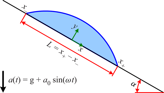
As a further application of the recent multiphase LB model with a self-tuning EOS and the present wetting condition treatment, a moving droplet on an inclined wall, which is vertically and sinusoidally oscillated, is simulated in this section. Since the inclined wall is ideally smooth and the contact angle hysteresis is not involved, it would be expected at first sight that the droplet will slide down under the effect of gravity. However, the experiments by Brunet, Eggers & Deegan (Reference Brunet, Eggers and Deegan2007) have shown that the droplet can actually climb up as long as the oscillation is sufficiently strong. For the sake of simulation, the coordinate system $(x , y)$ is fixed at the wall and an external acceleration $a_0 \sin (\omega t)$ is applied to mimic the wall oscillation, as shown in figure 16. Following Bradshaw & Billingham (Reference Bradshaw and Billingham2018), a dimensionless parameter $\epsilon$ is introduced to characterize the oscillation strength

(5.4)\begin{equation} \epsilon = \frac{ \rho_l a_0 L_0^2 \sin \alpha}{ \sigma_{lg} \theta_0} , \end{equation}

where $L_0$ is the distance between the two three-phase contact points of the static droplet on the wall in the absence of both gravitational and external accelerations, $\alpha$ is the inclination angle of the wall and $\theta _0$ is the static contact angle. The dimensionless angular frequency of the oscillation is defined as (Bradshaw & Billingham Reference Bradshaw and Billingham2018)

(5.5)\begin{equation} \hat{\omega} = \omega \sqrt{ \frac{\rho_l L_0^3 }{ \sigma_{lg} \theta_0 } } . \end{equation}

Similar to (5.4), the dimensionless acceleration due to gravity can be defined as

(5.6)\begin{equation} \hat{g} = \frac{ \rho_l g L_0^2 \sin \alpha}{ \sigma_{lg} \theta_0} , \end{equation}

where $g$ is the gravitational acceleration.

Figure 16.

Illustration of a moving droplet on an inclined wall, where the coordinate system $(x , y)$ is fixed at the wall and an external acceleration $a_0 \sin (\omega t)$ is applied to mimic the wall oscillation.

In the present simulations, the computational domain is chosen as $4096 \delta _x \times 512 \delta _x$. Periodic boundary conditions are applied in the $x$ direction, and solid walls are placed on both the lower and upper sides. A semicircular droplet is first deposited on the lower wall

(5.7a)\begin{gather} \rho (\boldsymbol{x} , 0) = \frac{ \rho_l + \rho_g }{2} - \frac{ \rho_l - \rho_g }{2} \tanh \frac{ |\boldsymbol{x} - \boldsymbol{x}_c| - R_0 }{ W_{lg} / \ln (19)} , \end{gather}

(5.7b)\begin{gather}\boldsymbol{u} (\boldsymbol{x}, 0) = \boldsymbol{0} , \end{gather}

where $\boldsymbol {x}_c = (2048 \delta _x, 0)^\mathrm {T}$ and $R_0 = 128 \delta _x$. Subsequently, an auxiliary simulation of the droplet wetting process is run to a steady state, which is then used as the initialization of the oscillation process. From this moment on (denoted as $t = 0$), the gravitational and external accelerations are turned on, and the droplet starts moving along the wall. The dimensionless relaxation time $\tau _f$ is changed from $1.5$ to $0.6$ to lower the viscous dissipation. The inclination angle of the wall and the static contact angle are chosen as $\alpha = 30^\circ$ and $\theta _0 = 45^\circ$, respectively. The parameter $\zeta$ in the tanh $\psi _s$ is set to $2$, and thus $\gamma = 0.0466517$ to make $\theta _0 = 45^\circ$. The dimensionless oscillation strength is set to $\epsilon = 4$, $8$ and $16$. The dimensionless angular frequency and gravitational acceleration are fixed at $\hat {\omega } = 1.6$ and $\hat {g} = 0.4$, respectively.

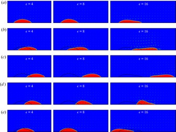
Figure 17 shows the snapshots of a moving droplet on an inclined wall, together with the velocity vector every $64$ points in both the $x$ and $y$ directions, at times $t / T_\textit {osi} = 19.00$, $19.25$, $19.50$, $19.75$ and $20.00$. Here, $T_\textit {osi} = 2 {\rm \pi}/ \omega$ is the oscillation period of the external acceleration and the effect of the initialization can be completely avoided after $19$ oscillation periods. At the beginning of the oscillation period ($t / T_\textit {osi} = 19.00$), the total acceleration, defined as $a = g + a_0 \sin (\omega t)$, satisfies $a = g$. A clockwise rotating vortex can be observed in the gas above the droplet, which slowly moves upward along the wall for $\epsilon = 4$, $8$ and $16$. The droplet shape is similar to a static droplet for $\epsilon = 4$ and $8$, while it is significantly stretched for $\epsilon = 16$. At the moment $t / T_\textit {osi} = 19.25$, the total acceleration gradually increases from $g$ to $g + a_0$. An anticlockwise rotating vortex can be clearly observed in the gas, and the droplet moves downward for all the involved $\epsilon$. It can be seen from figure 17(b) that the droplet is stretched slightly for $\epsilon = 4$ and more significantly as $\epsilon$ increases. At the moment $t / T_\textit {osi} = 19.50$, the total acceleration gradually decreases from $g + a_0$ to $g$. The anticlockwise rotating vortex in the gas is weakened as the downward movement of the droplet slows down due to the viscous dissipation. At the moment $t / T_\textit {osi} = 19.75$, the total acceleration further decreases from $g$ to $g - a_0$. Since $g / a_0 = \hat {g} / \epsilon \ll 1$, the total acceleration rapidly changes to the opposite direction of gravity during the third quarter of the oscillation period, and thus the droplet turns to move upward, which induces a clockwise rotating vortex in the gas. Comparing figure 17(b) with figure 17(d), it can be found that the maximum dynamic contact angle obtained at the upper three-phase contact point is larger than that obtained at the lower three-phase contact point. At the end of the oscillation period ($t / T_\textit {osi} = 20.00$), the total acceleration increases from $g - a_0$ to $g$. The velocity field and droplet shape are the same as those at the moment $t / T_\textit {osi} = 19.00$. As can be seen from figure 17(e), the net movement of the droplet within one oscillation period is sliding down for $\epsilon = 4$ but climbing up for $\epsilon = 8$ and $16$, and the net climbing up distance for $\epsilon = 16$ is much larger than that for $\epsilon = 8$. The above features captured by the present LB simulations are qualitatively consistent with the experiments by Brunet et al. (Reference Brunet, Eggers and Deegan2007) and the asymptotic analyses by Bradshaw & Billingham (Reference Bradshaw and Billingham2018).

Figure 17.

Snapshots of a moving droplet on an inclined wall, together with the velocity vector every $64$ points in both the $x$ and $y$ directions, during one oscillation period ((a) $t / T_\textit {osi} = 19.00$, (b) $t / T_\textit {osi} = 19.25$, (c) $t / T_\textit {osi} = 19.50$, (d) $t / T_\textit {osi} = 19.75$ and (e) $t / T_\textit {osi} = 20.00$) for $\epsilon = 4$, $8$ and $16$. The droplet profile at the beginning of the oscillation period ($t / T_\textit {osi} = 19.00$) is inserted into the snapshots at other moments ($t / T_\textit {osi} = 19.25$, $19.50$, $19.75$ and $20.00$).

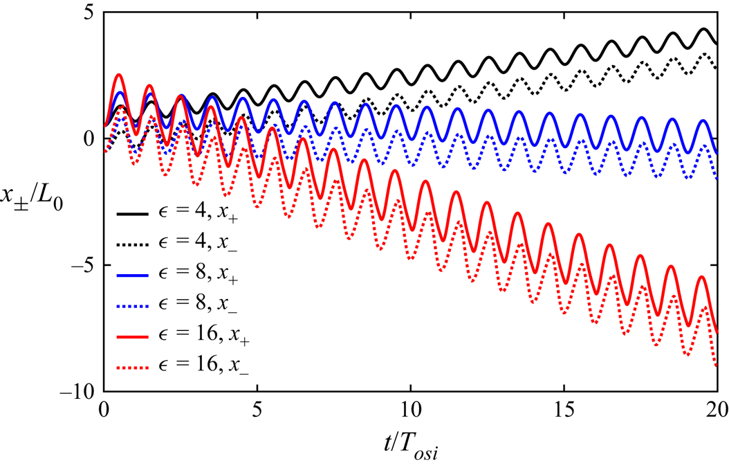
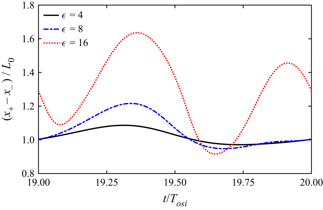
To better show the droplet movement, the time evolutions of the positions of the lower and upper three-phase contact points (denoted by $x_+$ and $x_-$, respectively, and normalized by $L_0$) are plotted in figure 18. As can be seen, both the lower and upper contact points periodically move downward and upward with the same frequency as the external acceleration, and the amplitude of such a periodic movement increases as $\epsilon$ is raised. For $\epsilon = 4$, that corresponds to a weak oscillation, the droplet slides down within one oscillation period, and the curves for $x_+ / L_0$ and $x_- / L_0$ are very similar but show a shift along the vertical axis, which indicates that the droplet deformation is small during the movement. For $\epsilon = 8$, that corresponds to a moderate oscillation, the droplet slowly climbs up within one oscillation period. As for $\epsilon = 16$, that corresponds to a strong oscillation, the droplet climbs up much faster, and a noticeable discrepancy between the shapes of the curves for $x_+ / L_0$ and $x_- / L_0$ can be observed. To be specific, $x_+ / L_0$ increases during $n + 0.054 \leq t / T_\textit {osi} \leq n + 0.486$ and decreases during $n + 0.486 \leq t / T_\textit {osi} \leq n + 1.054$, whereas $x_- / L_0$ increases during $n -0.002 \leq t / T_\textit {osi} \leq n + 0.580$ and decreases during $n + 0.580 \leq t / T_\textit {osi} \leq n + 0.998$. Here, $n$ denotes the $n \textrm {th}$ oscillation period. The discrepancy between the shapes of the curves for $x_+ / L_0$ and $x_- / L_0$ suggests that the droplet could shrink and spread twice within one oscillation period. Figure 19 shows the time evolutions of the distance between the lower and upper three-phase contact points (denoted by $L = x_+ - x_-$ and normalized by $L_0$) during one oscillation period ($n \leq t / T_\textit {osi} \leq n+1$ with $n = 19$), which confirms that the droplet shrinks and spreads twice for $\epsilon = 16$ but once for $\epsilon = 4$ and $8$ within one oscillation period. Meanwhile, the asymmetry of the curve for $(x_+ - x_-) / L_0$ between the downward and upward phases (i.e. between $n \leq t / T_\textit {osi} \leq n+0.5$ and $n+0.5 \leq t/T_\textit {osi} \leq n+1$), can be clearly observed from figure 19, which leads to the net climbing up movement caused by the periodic oscillation (Brunet et al. Reference Brunet, Eggers and Deegan2007; Noblin, Kofman & Celestini Reference Noblin, Kofman and Celestini2009).

Figure 18.

Time evolutions of the normalized positions of the lower and upper three-phase contact points $x_\pm / L_0$ for $\epsilon = 4$, $8$ and $16$.

Figure 19.

Time evolutions of the normalized distance between the lower and upper three-phase contact points $(x_+ - x_-) /L_0$ during one oscillation period ($19 \leq t /T_\textit {osi} \leq 20$) for $\epsilon = 4$, $8$ and $16$.

5.4. Droplet evaporation on adiabatic substrate

With the analysed surface thermodynamics and the thermodynamically consistent treatment for the wetting condition, we are now well equipped to simulate thermodynamic wetting problems involving liquid–vapour phase transition. The details of the extension of the multiphase LB model with a self-tuning EOS to liquid–vapour phase transition can be found in our previous work (Huang et al. Reference Huang, Wu and Adams2021), and in this section, the evaporation of a droplet on an adiabatic substrate is simulated to show the capability of the present wetting condition treatment. The computational domain is chosen as $1024 \delta _x \times 512 \delta _x$, and an adiabatic substrate with zero thickness is placed on its lower side (i.e. heat transfer inside the substrate is not considered). A semicircular droplet, given by (5.7) with $\boldsymbol {x}_c = (512 \delta _x, 0)^\mathrm {T}$ and $R_0 = 128 \delta _x$, is first deposited on the substrate, and an auxiliary simulation of the droplet wetting process is run to a steady state under isothermal conditions and this is then used as the initialization of the evaporation process. From this moment on (denoted as $t = 0$), a higher temperature $T_h = 0.9 T_\textit {cr}$, together with the outflow and constant-pressure condition, is applied to the other three sides of the computational domain to drive the evaporation process. The parameters $\zeta$ and $\gamma$ in the tanh $\psi _s$ are set to $2$ and $0.0329890$, respectively, to make the static contact angle $\theta _0 = 60^\circ$. The Stefan number, defined as $Ste = \rho _v c_v (T_h - T_0) / (\rho _l h_{lv})$, is chosen as $0.1$. Here, $T_0 = 0.8 T_\textit {cr}$ is the initial temperature, $\rho _l$ and $\rho _v$ are the saturated liquid and vapour densities at $T_0$, $c_v$ is the constant-volume specific heat and $h_{lv}$ is the latent heat of vaporization.

Figure 20 shows snapshots of the local temperature and velocity fields near the droplet, together with the streamlines inside the droplet, where the time is normalized as $t^\ast = \alpha _v t / L_0^2$ with $\alpha _v$ the thermal diffusivity of the vapour and $L_0$ the length of the droplet at time $t = 0$. In the evaporation process, the temperature in the vapour region gradually increases, while the temperature inside the droplet remains at the initial temperature $T_0 = 0.8 T_\textit {cr}$ due to the absorption of the latent heat. The vapour flows outside from the liquid–vapour interface, and the magnitude of the outflow velocity at the interface gradually increases as time goes on, which implies an increase in the evaporation flux. Meanwhile, two symmetric vortices with opposite rotations can be observed inside the droplet. This flow pattern is similar to that leading to the coffee-ring effect (Deegan et al. Reference Deegan, Bakajin, Dupont, Huber, Nagel and Witten1997), although the contact line in the present simulation is moving rather than pinned. The time evolutions of the droplet volume $V$, normalized by its initial value $V_0$, and dynamic contact angle $\theta$ are shown in figure 21. At the very early stage with $t^\ast < 0.125$, the droplet volume remains almost constant and the dynamic contact angle slightly increases, which are probably caused by the initialization of the evaporation process as the driving boundary conditions are abruptly applied to the other three sides. It can be observed from figure 21 that the droplet volume decreases approximately linearly with time, which means that the overall evaporation rate remains almost constant and thus the evaporation flux becomes more strongly singular during the droplet evaporation. This evaporating characteristic agrees with the previous theoretical and experimental findings for the case with a pinned contact line (Hu & Larson Reference Hu and Larson2002). Moreover, it is interesting to observe that the dynamic contact angle gradually decreases as the droplet evaporates, which can be explained by the increase of the recession velocity of the contact line due to the almost constant evaporation rate.

Figure 20.

Snapshots of the local temperature and velocity fields, as well as the streamlines inside the droplet, at different normalized times ((a) $t^\ast = 0.402$, (b) $t^\ast = 0.804$, (c) $t^\ast = 1.609$ and (d) $t^\ast = 2.316$) in the droplet evaporation process on an adiabatic substrate. The thick solid and dashed lines denote the droplet profile and its initial position, respectively.

Figure 21.

Evolutions of (a) the normalized droplet volume $V / V_0$ and (b) the dynamic contact angle $\theta$ with the normalized time $t^\ast$ in the droplet evaporation process on an adiabatic substrate. The moment when the droplet completely evaporates is denoted by the solid point.