





Highlights
What is already known?
-
• Sampling variances and small-sample bias corrections for effect sizes are usually obtained via delta-method expansions, which are hard to derive for non-statisticians.
-
• Parametric bootstrapping and ‘single-fit’ resampling have been proposed for inference, but their use for obtaining bias-corrected (BC) effect-size estimates and SEs in meta-analysis remains limited.
What is new?
-
• We formalise four steps (fit, draw, transform, and summarise) for the Single-fit, Accurate, Fast and Easy (SAFE) bootstrapping procedure, to obtain model-based BC point estimates and standard errors from reported summary statistics.
-
• We illustrate SAFE for common two-group designs using Gaussian working models for continuous outcomes and binomial (multinomial) models for discrete outcomes, including paired designs.
Potential impact for RSM readers
-
• We lower the technical barrier to introducing or adopting novel effect sizes and enable routine bias correction without new algebraic formulas.
-
• We provide a reproducible workflow that complements formula-based methods and makes their assumptions more transparent with code and an additional material (https://ejlundgren.github.io/SAFE/).
1. Introduction
More than four decades ago, statisticians realised that, instead of deriving sampling distributions with pencil-and-paper algebra, they could let the computer do the heavy lifting. With modern computing, one can repeatedly generate pseudo-data, recalculate the statistic of interest, and use the resulting distribution for inference. This broad family of approaches, often grouped under ‘bootstrapping’, has become influential in many disciplines, including meta-analysis.Reference Efron 1 – Reference Davison and Hinkley 4 However, not all bootstrap procedures are alike: some resample raw data non-parametrically, whereas others simulate from an explicitly assumed parametric model. Our focus here is on the latter.
Of relevance, formulas for common effect size statistics (e.g., standardised mean difference [SMD]) and their sampling variances are frequently used in meta-analysis. These formulas are often obtained via first- or second-order Taylor expansions, also known as the ‘delta method’.Reference Ver Hoef 5 Such formulas can be elegant and useful, but they may be difficult to derive for new statistics, difficult to verify, and sometimes inaccurate in small samples or under strong skewness. For many practitioners, the main practical problem is therefore not only how to derive a formula, but how to know whether the resulting approximation is adequate.
In this tutorial, we show how a parametric technique, termed Single-fit, Accurate, Fast, and Easy-to-implement (SAFE) bootstrapping, can provide model-based bias corrections and model-based standard errors (SEs) without requiring a new analytic derivation for every effect size. SAFE is not a non-parametric (assumption-free) bootstrap.Reference Efron 1 – Reference Davison and Hinkley 4 Rather, it is a bootstrap on summary statistics, conditional on an explicitly chosen sampling model. That is, SAFE works by fitting a simple sampling model once to the reported statistics, drawing many replicates under that model, transforming each replicate into the effect size of interest, and summarising the resulting bootstrap cloud. Its performance, therefore, depends on how well the assumed sampling model approximates the sampling distribution of the reported statistics.
The idea explored in this tutorial is not new, and previous papers have hinted at the power of this single-fit approach.Reference Mandel 6 , Reference Fletcher and Jowett 7 Our contribution is to organise it into a clear four-step workflow for meta-analytic effect sizes and to demonstrate it in settings commonly encountered by meta-analysts. Specifically, we focus on two-group designs that can be parameterised from standard reported summaries: Gaussian working models for continuous outcomes and binomial or multinomial models for discrete outcomes. We also emphasise that this tutorial mainly concerns effect sizes on transformed scales that are approximately unbounded and reasonably symmetric (e.g., log response ratio, log odds ratio [OR] and log risk ratio [RR]), because these are the settings in which the working models used here are most natural.
We begin with a simple example to make the SAFE bootstrap recipe accessible and concrete. Before moving to specific effect sizes, we also provide a brief practical guide summarising the designs covered here, the required summary statistics, and the working sampling models assumed. We then work through continuous-outcome effect sizes, namely the log response ratio and the SMD, including paired designs, before turning to discrete outcomes, such as log ORs and log RRs. We also illustrate less common metrics, such as the log coefficient-of-variation ratioReference Nakagawa, Poulin and Mengersen 8 , Reference Senior, Viechtbauer and Nakagawa 9 and the Hardy–Weinberg disequilibrium (HWD) statistic.Reference Wellek, Goddard and Ziegler 10 Throughout, we compare SAFE with familiar formula-based estimators and clarify when SAFE should be viewed as a useful practical alternative. An online supplement (https://ejlundgren.github.io/SAFE/) provides additional R code 11 and simulation results. Together, we hope that medical, biological, and social scientists, along with their students, can feel confident and ready to utilise this underappreciated yet broadly applicable method, which may encourage researchers to employ other simulation-based approaches more generally.
2. The concept and a simple example
2.1. Four steps to SAFEty
The SAFE bootstrap procedure is best understood in terms of four steps. Throughout, let
${\theta }$
 denote the effect-size statistic of interest. Importantly, every step below is conditional on an assumed sampling model for the reported summary statistics:
-
1. Fit: Choose a plausible sampling model for the observed data or summary statistics (e.g., a normal/Gaussian model for means or a Binomial model for counts) and estimate its parameters from the observed study. This step occurs only once and is therefore considered a ‘single-fit’ procedure. SAFE is therefore a parametric, model-based bootstrap on reported summary statistics, not a non-parametric bootstrap on raw data. Its validity depends on whether this working model provides a reasonable approximation to the sampling distribution of the statistics being used.
-
2. Draw: Generate a large batch of simulated summary statistics directly from the fitted model in one command (e.g., rnorm() or rbinom()). Under the assumed sampling model, each draw can be viewed as a credible representation of what might have been observed had the study been repeated under the same conditions.
-
3. Transform: Apply the effect-size formula to every simulated data set. Because transformations can be vectorised in software such as R, we turn tens of thousands of draws into tens of thousands of effect sizes very quickly.
-
4. Summarise: From the resulting vector of effect size estimates $\{\theta ^\ast \}$
 (or
$\boldsymbol {\theta }^* = \theta ^*_b,\ \text {for } b = 1, \dots , B$
; the vector
$\{\theta ^*\}$
sometimes referred to as a bootstrap cloud), we first quantify the standard deviation of the vector of effect size estimates, which is an estimate of the SE for the parameter, denoted as
$\mathrm {SE}_{\text {SAFE}}$
: (1) $$ \begin{align} \mathrm{SE}_{\text{SAFE}} \;=\; \text{sd}\!\big(\theta^\ast\big). \end{align} $$
Alternatively, we can calculate sampling variance as
(2) $$ \begin{align} \mathrm{Var}_{\text{SAFE}} \;=\; \text{var}\!\big(\theta^\ast\big). \end{align} $$
Then, we can quantify bias in the original effect size estimate ( $\hat \theta $
; the hat indicates that it is an estimate or estimator, an attempt to estimate the true values
$\theta $
, an estimand; note that, for example, Cohen’s
$d$
and Hedges’
$g$
are estimators of the standardised mean difference) by subtracting the original estimate from the mean of the vector of effect size estimates (
$\overline {\theta ^\ast }$
), simulated from Step 2: (3) $$ \begin{align} \widehat{\mathrm{bias}} \;=\; \overline{\theta^\ast}-\hat\theta. \end{align} $$
Using this estimated bias (an explanation of this formula is given below), we can obtain the bias-corrected (BC) point estimate, denoted as $\widehat {\theta }_{\mathrm {BC}}$
: (4) $$ \begin{align} \widehat{\theta}_{\mathrm{BC}} \;=\; \hat\theta - \widehat{\mathrm{bias}}. \end{align} $$
By combining Eqs. (3) and (4), we obtain
(5) $$ \begin{align} \widehat{\theta}_{\mathrm{BC}} \;=\; \hat\theta - \left(\overline{\theta^\ast}-\hat\theta\right) \;=\; 2\hat\theta - \overline{\theta^\ast}. \end{align} $$




These four steps are visualised in Figure 1 using a simple example presented in the next section.
Visualising four steps of the SAFE bootstrapping, using an example with a convex function,
$\mathbf {1 /x}$
 .
$S$
 signifies a small sample size case while
$L$
 a large sample size case; this schematics visualises why Jensen’s inequality has little impact on the large sample size case (for other symbols, see the main text). For why and how small-sample bias correction works, see also Figure 2.

Figure 1 Long description
The schematic is divided into four numbered steps.
* Step 1 Fit: Two normal distribution curves are shown on a horizontal axis. The left curve is wide and blue, labeled Small sample size S. The right curve is narrow and orange, labeled Large sample size L. Mathematical notation indicates x-bar star follows a normal distribution with mean mu and variance sigma-squared over n sub S or n sub L.
* Step 2 Draw: Below Step 1, multiple thin blue lines are drawn under the small sample distribution, and multiple thin orange lines under the large sample distribution, representing repeated sampling b equals 1 to B.
* Step 3 Transform: Located at the top right, a graph shows a convex function curve f(x) equals 1 over x-bar. Points from the x-axis are projected upward to the curve and then leftward to a vertical y-axis. The wide blue distribution from the x-axis transforms into a highly skewed, wider distribution on the y-axis. The narrow orange distribution transforms into a more symmetrical, narrower distribution on the y-axis, illustrating how Jensen's inequality affects small samples more than large ones.
* Step 4 Summarise: At the bottom, the distributions are compared. For the small sample size S, there is a visible gap labeled bias between the estimator theta-hat and the bias-corrected version theta-hat sub B C. For the large sample size L, shown in a box at the bottom, the values theta-hat sub B C, theta-hat, and theta-bar star are approximately equal. A central box notes that as n approaches infinity, all estimators become asymptotically equal. A final plot at the bottom right compares the sampling standard error of 1 over x-bar star, showing a much larger S D for the small sample size compared to the large sample size.
Bootstrap bias correction under convex versus concave transforms. Left panel: Three possible sampling distributions of the sample mean
$\bar x_1,\bar x_2,\bar x_3 \sim \mathcal N(\mu _i,\sigma ^2/n)$
 with identical spread (same SE) but different locations. Right panel: Applying (a) a convex transform (e.g.,
$f(x)=1/x$
 ) or (b) a concave transform (e.g.,
$f(x)=\ln x$
 ) bends these distributions. By Jensen’s inequality,
$E[f(\bar x)] \gtrless f(E[\bar x])$
 with ‘
$\ge $
 ’ for convex and ‘
$\le $
 ’ for concave, yielding an upward (a) or downward (b) bias. For each location
$i$
 , we simulate
$\{\bar x_i^{\ast }\}$
 , transform to
$\theta _i^{\ast }=f(\bar x_i^{\ast })$
 , and use
$\overline {\theta _i^{\ast }} \approx E[\hat \theta _i]$
 to estimate bias:
$\widehat {\mathrm {bias}}_i=\overline {\theta _i^{\ast }}-\hat \theta _i$
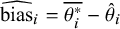 . The bias-corrected estimator is
$\hat \theta _{BC}=\hat \theta -\widehat {\mathrm {bias}}_i$
 . Because the three
$\bar x_i$
 distributions have the same SE, the bias (the distance between
$\overline {\theta _i^{\ast }}$
 and
$\hat \theta _i$
 ) is essentially the same across
$i$
 , even though the
$\bar x_i$
 (and thus
$\hat \theta _i=f(\bar x_i)$
 ) differ in location. In short, the bootstrap correction is driven by curvature and uncertainty, not by where
$\bar x$
 happens to sit.

Figure 2 Long description
The image is divided into a left section titled Normal and a right section titled Transform.
* Left Panel (Normal): Shows three overlapping bell-shaped normal distributions along a horizontal axis. They are colored green, orange, and blue from left to right, labeled x-bar sub 1, x-bar sub 2 (mu), and x-bar sub 3. Each has a vertical line marking its mean. Arrows point from this panel toward the right panels, indicating transformations.
* Top-Right Panel (a. Convex): Shows the three distributions after a 1/x transform. The curves are skewed. For each distribution, vertical lines indicate the transformed mean theta-hat sub i and the bootstrap mean theta-bar super star sub i. The distance between these lines is labeled as the bias estimate. A starburst callout near the center orange curve highlights the bias as the expected value of theta-hat minus theta. The bias is positive (upward) for all three locations.
* Bottom-Right Panel (b. Concave): Shows the distributions after a natural log transform. The curves are skewed in the opposite direction. Similar to the convex panel, vertical lines mark theta-hat sub i and theta-bar super star sub i. Here, the bias is negative (downward).
* Mathematical Summary: A box on the right side contains the formula theta-hat sub B C equals theta-hat minus (theta-bar super star sub i minus theta-hat sub i). It notes that the bias is approximately equal across all three distributions (bias sub x-bar sub 1 is approximately bias sub x-bar sub 2 is approximately bias sub x-bar sub 3) because the original distributions had the same standard error (S E).
The bias correction via SAFE is elegant in its simplicity.Reference Tibshirani and Efron
3
,
Reference Efron
12
Before understanding how this bias correction works, it is essential to comprehend how such a bias arises. Most meta-analytic effect sizes are non-linear transformations of the original (raw) statistics (e.g., mean and SD). When a transformation function
$f(\cdot )$
 is curved, the expected value of a transformed random variable (
$x$
 ) is not equal to the transformation of the variable’s expected value (also known as Jensen’s inequality):

Previous bias corrections for the log response ratio are essentially algebraic approximations to the same curvature-induced bias that SAFE estimates directly by simulation under the fitted sampling model.Reference Lajeunesse 13 By subtracting the estimated bias, we immediately obtain a second-order Taylor expansion correction that is often equivalent but without using the delta method. Importantly, when sample sizes are small, or uncertainty is large, this transformation-induced curvature bias can become non-negligible (Figure 1). SAFE is designed to estimate that bias directly, but only conditional on the chosen sampling model; if that model is misspecified, the estimated bias may also be misleading.
The key point is that SAFE estimates the bias of the plug-in estimator under the fitted sampling model. Let
$\hat \theta $
 denote the effect-size estimate computed from the observed summary statistics, and let
$\theta ^\ast _1,\ldots ,\theta ^\ast _B$
 denote the corresponding bootstrap replicates obtained after drawing from the fitted model and reapplying the same effect-size formula. The average bootstrap replicate,
$\overline {\theta ^\ast }=\frac {1}{B}\sum _{b=1}^B \theta ^\ast _b$
 , approximates the expected value of the estimator under the fitted model,
$E_{\mathrm {model}}(\hat \theta )$
 . Given this and the definition,
$\mathrm {bias} = E[\hat \theta ] - \theta $
 , the bootstrap estimate of bias is
$\widehat {\mathrm {bias}}_{\mathrm {SAFE}} = \overline {\theta ^\ast }-\hat \theta $
 , which estimates the difference between the model-based expectation of the estimator and the observed plug-in estimate. Subtracting this estimated bias gives the usual bootstrap BC estimator:
$\hat \theta _{\mathrm {BC}} = \hat \theta -\widehat {\mathrm {bias}}_{\mathrm {SAFE}} = 2\hat \theta -\overline {\theta ^\ast }$
 . Because this is a model-based bias correction, it does not directly estimate bias relative to an unknown true parameter; rather, it estimates the bias of the plug-in estimator under the assumed sampling model. Relatedly, SAFE is conditional on the fitted sampling model so that terms such as ‘accurate’, ‘bias-corrected’, and ‘standard error’ should be read throughout this tutorial as model-based. When the working model is poor, SAFE can also perform poorly; in that sense, SAFE complements rather than eliminates the need for statistical judgement.
Before presenting this example, we briefly note why our approach earns the acronym SAFE: Single-fit, Accurate, Fast, and Easy(-to-implement). It is because the procedure comprises: (i) single-fit with a sampling model using the data; (ii) accuracy through a bias-correction procedure; (iii) fast estimation as one vectorised simulation replaces thousands of re-fits; and (iv) an easy method, which, as we show below, can use the same four steps for any effect-size statistic. We return to each of these components as we work through our examples.
2.2. A simple example
Imagine an experiment to measure an insect’s performance in solving a maze (in seconds, denoted as
$x$
 ) with five insects. The mean completion time,
$\bar x$
 , is a measure of the latency to finish a maze, so the longer it takes, the worse the performance is. To make the readout more intuitive, we may wish to take the reciprocal of the mean, so larger values mean a faster time to completion (e.g., the reciprocal of 10 sec is 0.1 while 5 sec is 0.2). This reciprocal can then be considered as a measure of ‘speed’. Meta-analytically, we may wish to use this reciprocal,
$R$
 , as our new effect size statistic:

where
$\bar {x}$
 is the average of the time taken for maze completion for five insects. Based on this transformation, it is not immediately apparent how to calculate the sampling variance, or SE, for
$R$
 (speed). Further, because the reciprocal is a curved (convex) function, the plug-in estimate
$1/\bar x$
 is known to be upwardly-biased (i.e.,
$1/\bar x>$
 mean(1/
$x$
 )) and especially so in small samples (i.e., Jensen’s inequality). Now we apply our four-step SAFE procedure to
$R$
 (1/
$x$
 ) (Figure 1).
Step 1: Fit once. The sample mean (
$\bar x$
 ) has the following sampling distribution exactly when the underlying observations are normally distributed, and approximately so more generally by the central limit theorem when the observations are non-normal but the sample size is reasonably large:

where
$\bar x^*$
 indicates an instance of
$\bar x$
 ,
$\mu $
 is the population mean,
$\sigma ^2$
 is the population variance, and
$n$
 is the sample size. Using the observed sample, we plug in
$\mu \approx \bar x$
 and
$\sigma \approx \mathrm {sd}(x)$
 , so that the working model for the sampling distribution of the mean becomes
$\bar x^\ast \sim \mathcal N(\bar x,\, \mathrm {sd}(x)^2/n)$
 . Note that the standard deviation of
$\bar x^*$
 is
$\hat \sigma /\sqrt {n}$
 , not
$\hat \sigma $
 ; the latter being the population standard deviation and the former equivalent to the SE (i.e., the standard deviation of a sampled statistic). As mentioned above, SAFE deals with a distribution of parameters (e.g., mean), not raw data, which tend to be inaccessible to the meta-analyst.
Step 2: Draw once. We draw
$B$
 surrogate sample means from this normal approximation. Larger values of
$B$
 are better but computationally costly. We recommend
$B=100,000$
 , although
$B=1,000,000$
 could slightly improve performance, as validated in our simulation (https://ejlundgren.github.io/SAFE/), and offers an excellent balance between accuracy and efficiency.
Step 3: Transform once. Each surrogate mean is converted to
$R$
 (a speed) by taking its reciprocal.
Step 4: Summarise two metrics. We obtain BC point and SE estimates from bootstrapped data as follows:

The entire procedure is only a few lines of R code; note that crucially
$\text {sd}(x)\sqrt {n}$
 is used in the call to rnorm(), ensuring that we simulate data that follow the distribution of sample means:
set.seed(1)
x    <- c(11.3, 9.7, 10.4, 12.0, 9.1)    # five maze completion times
n    <- length(x)                        # number of observations in vector x
xbar <- mean(x)                          # calculate mean of observations
Rhat <- 1 / xbar                         # mean speed

## --- SAFE bootstrap ------------------------------------------------------
mu    <- xbar                            # mean time taken
sigma <- sd(x) / sqrt(n)                 # calculate SD of the mean
B     <- 1e6                             # 1 million bootstrap draws
x_star <- rnorm(B, mu, sigma)            # generating possible xbars (mean time taken)
R_star <- 1 / x_star                     # transform to speed

bias   <- mean(R_star) - Rhat            # bootstrap bias
R_BC   <- Rhat - bias                    # calculate bias-corrected speed
se_SFB <- sd(R_star)                     # calculate SAFE standard error

round(c(Rhat = Rhat, R_BC = R_BC, SE_SAFE = se_SFB), 4)
The console prints the following:
   Rhat    R_BC SE_SAFE
 0.0952  0.0950  0.0048
Three things are notable from this simple example. With a small sample size of five observations, SAFE delivers a bias correction of roughly 2%
$0.0952/0.0950 \approx 1.002$
 ; one can immediately see the degree to which such a correction matters. The SE emerges automatically; no delta-method derivation of
$\mathrm {Var}(1/\bar x)$
 is required. Nothing in the code is specific to the reciprocal itself. Replace the line R_star <- 1 / x_star with another transformation, such as an SMD or a log OR, and the same four-step logic still applies. What changes is the required sampling model for the summary statistics entering that transformation. Accordingly, SAFE yields a BC estimate and an SE under the assumed sampling model, rather than a universally valid SE irrespective of model choice (for simulation validation, see our additional material: https://ejlundgren.github.io/SAFE/); incidentally, the delta-method-based variance for
$R$
 is
$\text {var}(R) = s^2/(n\bar x^4)$
 .
Before turning to specific examples, it is useful to state the practical scope of this tutorial. Here, we focus on effect sizes for two-group designs that can be computed from standard reported summaries (means, standard deviations, sample sizes, and cell counts). In the continuous examples, we use Gaussian working models for sample means and, where needed, for sample variances or related quantities. In the discrete examples, we use binomial or multinomial working models for counts.
3. Effect sizes for continuous outcomes
In this section, we show how the same four-step SAFE logic extends to effect-size statistics for continuous outcomes comparing two groups, namely the log response ratio (ratio of means) and the standardised mean difference. First, we consider two independent groups, and then two dependent groups (paired, matched, or crossover design).
3.1. Response ratio (ratio of means: lnRoM)
The so-called response ratio (log response ratio; also known as the log ratio of means) was first proposed by Hedges et al.Reference Hedges, Gurevitch and Curtis
14
as an alternative to the SMD, which we denote as lnRoM. We note that the acronym lnRR is commonly used, but in this article, we reserve it for the log risk ratio presented in the next section. Imagine two groups, Group 1 (
$\bar x_1 ,\, s_1 ,\, n_1$
 ; sample mean, standard deviation, and sample size) and Group 2 (
$\bar x_2 ,\, s_2 ,\, n_2$
 ). The original log response ratio can be written as

This is the definition formula for lnRoM; such formulas are often referred to as ‘plug-ins’. A first-order Taylor expansion gives the sampling variance as

Note that we label this combination of Eqs. (8) and (9) as ‘First’ in our R scripts and this tutorial, although Eq. (9) was not derived using the delta method and the first-order Taylor expansion. Later LajeunesseReference Lajeunesse 13 improved both point and variance estimates by using second-order Taylor expansions (which we label as ‘Second’), which are as follows:


For SAFE bootstrapping, we treat the pair of sample means as a bivariate normal distribution:

At this stage, one could use two independent normal distributions (i.e., rnorm() twice). However, the multivariate normal distribution has an advantage, which we will show later. A single call to mvrnorm() from the MASS packageReference Venables and Ripley
15
draws
$B$
 pairs
$(\bar x_1^{\ast },\bar x_2^{\ast })$
 ; we transform each into
$\ln (\bar x_1^{\ast }/\bar x_2^{\ast })$
 in one vectorised step, then compute

Under this Gaussian working model, simulated means may occasionally fall below zero, which is incompatible with the log transformation. In practice, however, this issue is typically negligible when the observed means are largely positive relative to their sampling variation, making negative draws rare. More importantly, the multivariate normal formulation is convenient because it generalises naturally to settings where the two sample means are correlated, such as paired or otherwise dependent designs. We therefore use mvrnorm() as the default working model throughout, while recognising that its suitability depends on the probability of implausible negative draws being very small (note that we need to remove such negative values for the SAFE procedures.
Below is an example R code in which we compare SAFE estimates with estimates from the formulas in Eqs. (8) through (11). Estimates from the second-order delta method are generally considered more accurate than those from the first-order counterpart, and we expect the SAFE estimates to be similar to the second-order estimates.
set.seed(7)
## Example data (means, SDs, sample sizes) ------------------------------
x1 <- 13.4;  s1 <- 4.6;  n1 <- 18          # group 1
x2 <- 16.1;  s2 <- 3.9;  n2 <- 17          # group 2

## 1. FIRST-order (plug-in) lnRoM & SE  ---------------------------------
theta_First <- log(x1 / x2)                               # Eq. 8
var_First   <-  s1^2/(n1 * x1^2) + s2^2/(n2 * x2^2)       # Eq. 9
se_First    <- sqrt(var_First)

## 2. SECOND-order lnRoM & SE  ----------------------------------
theta_Second <- log(x1 / x2) +
                0.5 * ( s1^2/(n1 * x1^2) - s2^2/(n2 * x2^2) )  # Eq. 10

var_Second <- var_First +
              0.5 * ( s1^4/(n1^2 * x1^4) + s2^4/(n2^2 * x2^4) ) # Eq.11
se_Second  <- sqrt(var_Second)

## 3. SAFE single-fit bootstrap (multivariate Normal) -------------------
library(MASS)
mu  <- c(m1 = x1, m2 = x2)
Sig <- diag(c(s1^2/n1, s2^2/n2))            # independent sample means
B   <- 1e6                                  # number of bootstrap draws
draw <- mvrnorm(B, mu, Sig)                 # Fit-once, draw-once
theta_star <- log(draw[,"m1"] / draw[,"m2"])# Transform-once

se_SAFE       <- sd(theta_star)             # first summary: SE
bias_SAFE     <- mean(theta_star) - theta_First
theta_SAFE_BC <- theta_First - bias_SAFE    # second summary: BC point

## 4. Print tidy comparison ---------------------------------------------
results <- rbind(  Point = c(First  = theta_First,
            Second = theta_Second,
            SAFE   = theta_SAFE_BC),
  SE    = c(First  = se_First,
            Second = se_Second,
            SAFE   = se_SAFE)
)
round(results, 4)
When you run the code, the console returns something like the following, where First represents estimates from Eqs. (8) and (9), Second represents estimates from Eqs. (10) and (11), and SAFE represents estimates from the SAFE bootstrapping.
        First  Second    SAFE
Point -0.1836 -0.1820 -0.1820
SE     0.1000  0.1001  0.1007
As you see, the point estimates from the second column (the second-order correction formulas; Eqs. (10) and (11)) and the third column (SAFE bootstrap) match well, although SE from SAFE is slightly larger. In contrast, the point estimate from the first column (Eqs. (8) and (9)) deviates from the other two. Note that
$\text {SE}_{\text {SAFE}}$
 can be slightly larger in small samples, which usually results in higher coverages (the coverages are presented in an additional material: https://ejlundgren.github.io/SAFE/).
3.2. Standardised mean difference (SMD)
The SMD remains extremely popular for continuous outcomes in ecology, psychology, and medicine. SMD may also be often referred to as Cohen’s
$d$
 or Hedges’
$g$
 , both of which are estimators of SMD. Although Cohen seems to have introduced SMD first,Reference Cohen
16
HedgesReference Hedges
17
was the first to formalise SMD with its sampling variance. As with lnRoM, we have two independent groups with summary statistics: Group 1 (
$\bar x_{1},\, s_{1},\, n_{1}$
 ) and Group 2 (
$\bar x_{2},\, s_{2},\, n_{2}$
 ). Following Borenstein et al.,Reference Borenstein, Hedges, Higgins and Rothstein
18
we can define Cohen’s
$d$
 as

where the term
$n_{1}+n_{2}-2$
 is often referred to as the degree of freedom (
$df$
 ). The sampling variance for SMD is

We note that this variance formula can be traced back to Hedges,Reference Hedges
17
who notably used the non-central
$t$
 distribution in its derivation, rather than the delta method, which is commonly used elsewhere. HedgesReference Hedges
17
recognised that, for small samples, the expectation of
$d$
 is slightly inflated.Reference Hedges
19
,
Reference Hedges and Olkin
20
Multiplying by the correction factor:

can alleviate this inflation; the resulting so-called Hedges’
$g$
 can be written as

And, therefore, the sampling variance of
$g$
 is

Given that SMD includes the sample standard deviation (
$s_{\text {p}}$
 or variance
$s^2_{\text {p}}$
 ), we need to know the sampling variance of the variance estimate, which, assuming variances are normally distributed, isReference Anderson
21
:

We note that variance is bounded at zero, and so when the variance is close to zero, the assumption of normality is impractical. For such cases, we discuss an alternate estimator below.
We also note that the SAFE bootstrap of SMD is by far the most challenging among those presented in this article. Now, for the SAFE procedure, we sample the quartet
$\big (\bar X_{1},\bar X_{2},S^{2}_{1},S^{2}_{2}\big )$
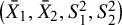 jointly:

Off-diagonal elements of
$\Sigma $
 are zero because the two groups are assumed independent. In addition, for independently and identically distributed (i.i.d.) normal data, the sample mean, and sample variance are independent, which motivates the block-diagonal form used here. As before, using mvrnorm(), we draw
$B$
 independent replicates of the quartet: (
$\bar x_{1}^*,\;\bar x_{2}^*,\;s_{1}^{2*},\;s_{2}^{2*}$
 ), Then, we vectorise the usual pooled-variance formula and compute
$d$
 using Eq. (12). A more principled alternative is to sample variance components from their exact or more natural positive-support distributions, such as
$\chi ^2$
 distributions (or the Wishart distribution in multivariate settings), rather than from a Gaussian approximation. These approaches avoid impossible negative variance draws and are likely preferable when implementing SAFE for statistics that depend directly on sample variances. For simplicity, however, we retain the Gaussian working model here and return to this issue in an additional material (https://ejlundgren.github.io/SAFE/).
From this vector of
$d^*$
 values, we read off:

Below is an R example where we implement formulas for
$d$
 and
$g$
 along with the SAFE procedure.
set.seed(11)
## 0. Example data --------------------------------------------------------
x1 <- 13.4; s1 <- 4.6; n1 <- 18 # group 1
x2 <- 16.1; s2 <- 3.9; n2 <- 17 # group 2
df <- n1 + n2 - 2               # degrees of freedom required for sp2

## 1. Plug-in Cohen d & delta-method SE -----------------------------------
sp2    <- ((n1-1)*s1^2 + (n2-1)*s2^2) / df
d_hat  <- (x1 - x2) / sqrt(sp2)            # Eq. 12
Var_d  <- (n1+n2)/(n1*n2) + d_hat^2/(2*df) # Eq. 13
se_delta <- sqrt(Var_d)

## 2. Hedges' g & its SE --------------------------------------------------
J      <- 1 - 3/(4*df - 1)
g_hat  <- J * d_hat                        # Eq. 15
Var_g  <- J^2 * Var_d                      # Eq. 16
se_g   <- sqrt(Var_g)

## 3. SAFE bootstrap on d (4-variate) -------------------------------------
library(MASS)
mu    <- c(X1=x1, X2=x2, V1=s1^2, V2=s2^2)
Sigma <- matrix(0, 4, 4)
diag(Sigma) <- c(s1^2/n1, s2^2/n2,
                 2*s1^4/(n1-1), 2*s2^4/(n2-1))
B      <- 1e6    # the number of bootstrap
draw   <- mvrnorm(B, mu, Sigma)

# reject negative variances
draw <- draw[draw[,"V1"]>0 & draw[,"V2"]>0, ]

sp2_star <- ((n1-1)*draw[,"V1"] + (n2-1)*draw[,"V2"]) / df
d_star   <- (draw[,"X1"] - draw[,"X2"]) / sqrt(sp2_star)

se_SAFE  <- sd(d_star)
bias     <- mean(d_star) - d_hat
d_BC     <- d_hat - bias

## 4. Compare -------------------------------------------------------------
res <- rbind(  Point = c(d   = d_hat,  g   = g_hat,  SAFE = d_BC),
  SE    = c(d =se_delta,  g   = se_g,   SAFE = se_SAFE)
)
round(res, 4)
We get the following in the console:
            d       g    SAFE
Point -0.6316 -0.6171 -0.6156
SE     0.3470  0.3391  0.3613
We observe that the BC
$d$
 via SAFE is closer to
$g$
 than to the uncorrected
$d$
 in this example. Also,
$\text {SE}_{\text {SAFE}}$
 is somewhat larger here than the formula-based alternatives. Again, this should not automatically be interpreted as undue conservatism: simulation-based SEs can reflect higher-order uncertainty induced by the non-linear transformation, especially in smaller samples. A full simulation comparison is given in an additional material (https://ejlundgren.github.io/SAFE/); in that simulation, we see that the use of Wishart distributions produces better point and variance estimators than an assumed normal distribution. We also find the SE for
$d$
 (Eq. (13)) seems to perform best in combination with Hedge’s
$g$
 , and notably, escalc() from the metafor packageReference Viechtbauer
22
uses this combination.
3.3. Matched (paired) designs or repeated measures
Many experiments measure the same individuals twice: before/after a treatment, or under two conditions. These designs are known to be more powerful because the SE can be smaller than an independent design. This is because the within-pair correlation
$r$
 can reduce the sampling variance. This reduction can be seen in action in the formula for the sampling variance for lnRoM for dependent cases (denoted by the subscript ‘D’)Reference Lajeunesse
23
:

Note that the within-pair correlation
$r$
 is ideally estimated from the original study, but is often not reported. In such cases, analysts may need to assume a plausible value (e.g.,
$r=0.5$
 ).Reference Noble, Lagisz, O’dea and Nakagawa
24
However, because both formula-based and SAFE estimates can depend on this assumption, we recommend conducting sensitivity analyses over a range of plausible
$r$
 values and reporting how the point estimate and sampling variance change across that range along how model estimates change. The formula for the point estimate for dependent lnRoM is as above (Eq. (8)). Also, with a paired design,
$n_1 = n_2 = n$
 .
To estimate the bias-adjusted point estimates and sampling variances for dependent lnRoM via SAFE, we simply need to adjust the assumed distribution of the sample statistics in the ‘fit’ step to incorporate the correlation (as covariance) into the bivariate normal distribution from which we draw our samples as

From here, the remaining steps for SAFE estimation are identical to the independent case of lnRoM.
Similarly, there are sampling variance formulas for dependent SMD cases.Reference Becker 25 , Reference Morris 26 However, again, we can use SAFE for estimation by specifying the joint sampling distribution of the two group means and their sample variances by a quartet-variate normal with covariances.Reference Senior, Viechtbauer and Nakagawa 9 A slight complication is that we need to know the sampling covariance of two variances, which is defined asReference Anderson 21 :

where
$\rho $
 is the true value for an estimated within-pair correlation
$r$
 .
In the fit step of SAFE, we then draw once from

Again, the rest of the SAFE procedure remains the same, with the notable exception that
$n_1 = n_2 = n$
 . In summary, for dependent effect sizes, once the correlation
$r$
 is incorporated into the covariance matrix for the ‘fit’ step, the four SAFE steps remain unchanged.
4. Effect sizes for discrete outcomes
Having shown that SAFE handles continuous-outcome effect sizes, we now move to discrete-outcome effect size statistics, namely ORs and RRs. We again use the same four steps, but the sampling model consists of a pair of independent binomial distributions. We also show how to use a continuity correction (e.g., adding
$0.5$
 to every cell value) when zero counts exist.
4.1. Odds ratio (lnOR)
Many studies report a binary outcome (e.g., survived/died, chose patch A/patch B). For two independent groups, we obtain the
$2\times 2$
 table of counts, as

with sample risks
$\hat p_{1}=a/n_{1}$
 and
$\hat p_{2}=c/n_{2}$
 . Using these four cells, we can define the log OR as

which is a very popular effect size for this type of data.
Under a first-order Taylor expansion, the sample variance for the lnOR isReference Woolf 27 , Reference Agresti 28 :

However, this formula fails whenever
$a,b,c$
 , or
$d$
 equals
$0$
 , as we cannot divide by
$0$
 . A popular workaround is the ‘continuity correction’Reference Yates
29
with

applied before both the point estimate and variance are evaluated. In settings with zero cells, this means that the practical target of inference is no longer the uncorrected
$\ln \mathrm {OR}$
 , but rather the continuity-corrected log OR estimator. Accordingly, when SAFE is used with this correction, it estimates the bias and sampling variance of that corrected estimator.
As mentioned earlier, for SAFE, we model events in each group as independent draws from two binomial distributions, as

drawing
$B$
 (bootstrap) replicates
$(a^{\ast },c^{\ast })$
 . Equivalently, each group can be viewed as a two-category multinomial sample with a fixed row total, so that the non-event counts are determined automatically as
$b^\ast =n_1-a^\ast $
 and
$d^\ast =n_2-c^\ast $
 . Then, we transform each pair into a continuity-corrected bootstrap OR:

where the
$\delta $
 terms are zero unless a continuity correction is invoked for that replicate (e.g.,
$\delta =0.5$
 when any cell is zero).
The vector of
$\ln \mathrm {OR}^{\ast }_{\mathrm {CC}}$
 gives

Here, the subscript
$\mathrm {CC}$
 indicates that the same continuity-correction rule used for the observed estimator is also applied within the bootstrap replicates whenever needed. Below is an example R script with a continuity correction of 0.5 to handle zero cells in draws.
set.seed(24)

## 0. Observed 2x2 table (a b | c d) -----------------------------
a <- 2 ; b <- 20            #  2 / 22 events in Group 1
c <- 10; d <- 12            # 10 / 22 events in Group 2
n1 <- a + b
n2 <- c + d

## 1. Plug-in lnOR (no +0.5 since no zero cells) -----------------
theta_plug <- log((a * d) / (b * c))    # Eq. 20

## the delta-method SE
var_delta <- 1/a + 1/b + 1/c + 1/d      # Eq. 21
se_delta  <- sqrt(var_delta)

## 2. SAFE single-fit bootstrap (Binomial) ----------------
B <- 1e6                                # bootstrap no.
a_star <- rbinom(B, n1, a / n1)         # events  in Group 1
c_star <- rbinom(B, n2, c / n2)         # events  in Group 2
b_star <- n1 - a_star                   # non-events G1
d_star <- n2 - c_star                   # non-events G2

## Apply +0.5 only to rows with ANY zero count -------------------
needs_cc <- (a_star == 0 | b_star == 0 | c_star == 0 | d_star == 0)
a_star[needs_cc] <- a_star[needs_cc] + 0.5
b_star[needs_cc] <- b_star[needs_cc] + 0.5
c_star[needs_cc] <- c_star[needs_cc] + 0.5
d_star[needs_cc] <- d_star[needs_cc] + 0.5

theta_star <- log((a_star * d_star) / (b_star * c_star))

## 3. SAFE summaries --------------------------------------------
se_SAFE  <- sd(theta_star)
bias_hat <- mean(theta_star) - theta_plug
theta_BC <- theta_plug - bias_hat      # bias-corrected lnOR

## 4. Nicely formatted output -----------------------------------
out <- rbind(  Point = c(First = theta_plug,
            SAFE    = theta_BC),
  SE    = c(First   = se_delta,
            SAFE    = se_SAFE)
)
print( round(out, 4) )
Running this script should yield the following results:
        First    SAFE
Point -2.1203 -1.9515
SE     0.8563  0.8714
Both procedures provide comparable point and variance estimates, and their discrepancies disappear as sample sizes increase (see supporting simulation).
4.2. Relative risk (risk ratio: lnRR)
For discrete outcomes, many authors also use the relative risk, also known as the RR. Using the 2
$\times $
 2 contingency table above, the log RR can be defined as

A first-order Taylor expansion for the sampling variance of the observed lnRR,Reference Agresti
28
,
Reference Bailey
30
where
$p_{1}=a/n_{1}$
 and
$p_{2}=c/n_{2}$
 , is

This expression fails whenever
$a=0$
 or
$c=0$
 . In practice, a continuity correction is then often applied by adding
$0.5$
 to the event and non-event counts within the affected group before evaluating the point estimate and variance. Consequently, when zero-event cells are present, the practical target of inference is the continuity-corrected log RR estimator, rather than the uncorrected lnRR itself. Accordingly, when SAFE is implemented with this correction, it estimates the bias and sampling variance of that corrected estimator.
For the SAFE procedure, a single call to rbinom() for each group suffices just as lnOR above:

with
$b^\ast =n_{1}-a^\ast $
 and
$d^\ast =n_{2}-c^\ast $
 filled in by definition. The four SAFE moves: fit, draw, transform, and summarise, then yield:

As before, the subscript
$\mathrm {CC}$
 indicates that the same continuity-correction rule used for the observed estimator is also applied within the bootstrap replicates whenever needed. Below is an R example for lnRR with continuity correction of 0.5, comparing formula-based and simulation-based methods.
set.seed(24)

## 0) Observed 2x2 table (a b | c d) ---------------------------------
a <- 2 ; b <- 20            #  2 / 22 events in Group 1
c <- 10; d <- 12            # 10 / 22 events in Group 2
n1 <- a + b
n2 <- c + d
p1 <- a / n1
p2 <- c / n2

## 1) FIRST-order (plug-in) lnRR & delta SE ---------------------------
theta_First <- log(p1 / p2)                   # Eq. 22
var_First   <- (1 - p1) / a + (1 - p2) / c    # Eq. 23
se_First    <- sqrt(var_First)

## 2) SAFE single-fit bootstrap (Binomial) ----------------------------
B <- 1e6
a_star <- rbinom(B, n1, p1)
c_star <- rbinom(B, n2, p2)
## success-only continuity correction per replicate where needed
add <- 0.5
add1 <- ifelse(a_star == 0, add, 0)
add2 <- ifelse(c_star == 0, add, 0)

p1_star <- (a_star + add1) / (n1 + 2 * add1)   # if a_star==0 -> denom n1+1
p2_star <- (c_star + add2) / (n2 + 2 * add2)   # if c_star==0 -> denom n2+1

theta_star <- log(p1_star / p2_star)
theta_star <- theta_star[is.finite(theta_star)]  # safety

se_SAFE    <- sd(theta_star)
bias_SAFE  <- mean(theta_star) - theta_First
theta_SAFE <- theta_First - bias_SAFE            # bias-corrected point

## 3) Nicely formatted comparison ------------------------------------
out_lnRR <- rbind(  Point = c(First = theta_First,
            SAFE  = theta_SAFE),
  SE    = c(First = se_First,
            SAFE  = se_SAFE)
)
print(round(out_lnRR, 4))
We obtain the following:
        First    SAFE
Point -1.6094 -1.4571
SE     0.7135  0.7277
The bootstrap SE is slightly larger, and the BC point is pulled closer to zero. Our simulation suggests that the SAFE procedure tends to give more accurate estimates. Also, it is noteworthy that for both lnOR and lnRR, we could have used a multivariate normal to sample using modelling risks:
$p_{1}$
 and
$p_{2}$
 and their sampling variances
$p_{1}(1-p_{1})/n_1$
 and
$p_{2}(1-p_{2})/n_2$
 (for an example, see an additional material: https://ejlundgren.github.io/SAFE/).
5. Less common effect sizes
In this section, we apply the SAFE bootstrap to two lesser-known effect-size statistics to demonstrate its broad applicability.
5.1. Log coefficient-of-variation ratio (lnCVR)
The coefficient of variation (CV) is defined as the ratio of the standard deviation to the mean,
$\mathrm {CV}=s/\bar {x}$
 . When comparing two groups in terms of variability (CV), the log CV ratio is useful, as proposed by Nakagawa et al.Reference Nakagawa, Poulin and Mengersen
8
:

A first-order delta-method approximation for its variance:

This accounts for both the uncertainty in the means and the sample standard deviations.
Subsequently, Senior et al.Reference Senior, Viechtbauer and Nakagawa 9 proposed second-order versions of both point and variance estimates as follows:


They also proposed dependent cases, both the first- and second-order versions of sampling variances (D1 and D2, respectively), as follows:


SAFE does not require these complex formulas; we can use the quartet with the covariances between the two means and between the two variances, where
$r$
 is 0 for independent groups and
$r> 0$
 for dependent cases (paired or matched-case designs):

As with SMD, this implementation is conditional on a Gaussian working model for the sample means and sample variances; therefore, negative variance draws or strongly skewed positive outcomes indicate that a different sampling model may be preferable.
For each of
$B$
 draws, we compute

The SAFE summaries are

Below are two examples, one assuming
$r = 0$
 (two independent groups) and the other
$r = 0.5$
 (two paired groups with a correlation of 0.5). In this instance, we create an R function that handles the independent and dependent scenarios more flexibly.
set.seed(1234)
library(MASS)

safe_lncvr <- function(x1, s1, n1, x2, s2, n2, r = 0, B = 1e6) {
  # --- Point estimates --------------------------------------------------
  lnCVR1 <- log(s1 / x1) - log(s2 / x2)            # Eq. 24
  lnCVR2 <- lnCVR1 +
    0.5 * (1/(n1 - 1) - 1/(n2 - 1)) +
    0.5 * (s2^2/(n2 * x2^2) - s1^2/(n1 * x1^2))    # Eq. 26

  # --- Variance formulas (incorporating r) ------------------------------
  if (r == 0) {
    # independent groups
    var1 <- s1^2/(n1 * x1^2) + s2^2/(n2 * x2^2) +
            1/(2*(n1 - 1))      + 1/(2*(n2 - 1))   # Eq. 25
    var2 <- s1^2/(n1 * x1^2) + s1^4/(2 * n1^2 * x1^4) + n1/(2*(n1 - 1)^2) +
            s2^2/(n2 * x2^2) + s2^4/(2 * n2^2 * x2^4) + n2/(2*(n2 - 1)^2)
                                                   # Eq. 27
  } else {
    # dependent (paired) case, assume n1 = n2 = n
    n <- n1
    var1 <- s1^2/(n * x1^2) + s2^2/(n * x2^2) -
            2*r*s1*s2/(n * x1 * x2) +
            1/(n - 1) - r^2/(n - 1)                # Eq. 28
    var2 <- s1^2/(n * x1^2) + s1^4/(2 * n^2 * x1^4) +
            s2^2/(n * x2^2) + s2^4/(2 * n^2 * x2^4) -
            2*r*s1*s2/(n * x1 * x2) +
            r^2 * s1^2 * s2^2 * (x1^4 + x2^4) / (2 * n^2 * x1^4 * x2^4) +
            n/(n - 1)^2 - r^2/(n - 1) +
            r^4 * (s1^8 + s2^8) / (2 * (n - 1)^2 * s1^4 * s2^4)
                                                   # Eq. 29
  }
  se1 <- sqrt(var1)
  se2 <- sqrt(var2)

  # --- SAFE bootstrap for bias correction ------------------------------
  mu <- c(x1, x2, s1^2, s2^2)
  Sigma <- matrix(0, 4, 4)
  Sigma[1,1] <- s1^2 / n1
  Sigma[2,2] <- s2^2 / n2
  Sigma[1,2] <- Sigma[2,1] <- r * s1 * s2 / sqrt(n1 * n2)
  Sigma[3,3] <- 2 * s1^4 / (n1 - 1)
  Sigma[4,4] <- 2 * s2^4 / (n2 - 1)
  Sigma[3,4] <- Sigma[4,3] <- 2 * r^2 * s1^2 * s2^2 / sqrt((n1 - 1)*(n2 - 1))

  draws <- MASS::mvrnorm(B, mu, Sigma)
  draws <- draws[draws[,3] > 0 & draws[,4] > 0, ]
  X1s <- draws[,1]; X2s <- draws[,2]
  S1s <- sqrt(draws[,3]); S2s <- sqrt(draws[,4])
  theta_star <- log(S1s / X1s) - log(S2s / X2s)
  se_safe <- sd(theta_star)
  bias    <- mean(theta_star) - lnCVR1
  lnCVR_bc <- lnCVR1 - bias

  c(First     = lnCVR1,
    Second    = lnCVR2,
    SAFE_BC   = lnCVR_bc,
    SE_First  = se1,
    SE_Second = se2,
    SE_SAFE   = se_safe)
}

# --- Examples -------------------------------------------------------

# Independent groups (r = 0) n can be different between two groups
res_ind <- safe_lncvr(x1 = 17, s1 = 2, n1 = 23,
                      x2 =  12, s2 = 3, n2 = 27,
                      r  = 0)

# Paired design (r = 0.5; n1 = n2 = 25) n needs to be the same
res_dep <- safe_lncvr(x1 = 15, s1 = 2, n1 = 25,
                      x2 = 10, s2 = 2, n2 = 25,
                      r  = 0.5)

# Organise into tables -----------------------------------------------
tab_ind <- rbind(  Point = res_ind[c("First","Second","SAFE")],
  SE    = res_ind[c("SE_First","SE_Second","SE_SAFE")]
)
tab_dep <- rbind(  Point = res_dep[c("First","Second","SAFE")],
  SE    = res_dep[c("SE_First","SE_Second","SE_SAFE")]
)
We should get the following (first, the independent case, and then the dependent case):
> round(tab_ind, 4)
        First  Second    SAFE
Point -0.7538 -0.7494 -0.7479
SE     0.2118  0.2160  0.2453
> round(tab_dep, 4)
        First  Second    SAFE
Point -0.4055 -0.4050 -0.4052
SE     0.1803  0.1853  0.2112
This appears to be the most complex script so far, but the principles and SAFE steps remain the same. As above, the second-order delta method yields point estimates similar to those from SAFE.
5.2. Hardy–Weinberg disequilibrium
In population genetics, the Hardy–Weinberg equilibrium (HWE) at a bi-allelic locus implies that observed genotype counts
$\,n_{AA},n_{Aa},n_{aa}\,$
 in a sample of size
$n=n_{AA}+n_{Aa}+n_{aa}$
 follow proportions
$ p_1=n_{AA}/n,\;p_2=n_{Aa}/n,\; p_3=n_{aa}/n$
 with
$p_1+ p_2+ p_3=1$
 . The allele frequency of
$A$
 is

so the expected heterozygote proportion under HWE is
$2 p(1- p)$
 .
We quantify departure from HWE (HWD) using the relative excess of heterozygosity index as a measure of HWD,Reference Wellek, Goddard and Ziegler 10 which compares the observed heterozygosity to a symmetric homozygote-based benchmark:

This equals
$0$
 under exact HWE (since
$2\sqrt {p_1 p_3}=2p(1-p)$
 at HWE) and is label-invariant with respect to
$AA$
 and
$aa$
 .
A first-order delta-method approximation for the sampling variance of
$\ln \omega $
 is

As you can see, these equations (Eqs. (30) and (31)) are undefined when
$ p_1=0,\;p_2=0,\; \text {and} \:p_3=0$
 , and as lnOR and lnRR, we can add 0.5 in such cases (i.e., continuity correction).
To generate SAFE estimates of the departure from HWE, we model genotype counts as a single draw from a multinomial distribution:

Then, for each of
$B$
 replicates, compute

The SE for the effect size can then be found as

Below is an example implemented in R:
set.seed(123)

## --- observed data -------------------------------------------------
nAA <- 40; nAa <- 25; naa <- 50
n   <- nAA + nAa + naa

## --- continuity correction (CC) settings ---------------------------
add <- 0.5

## --- apply CC to observed counts only if any zero ------------------
add_obs   <- if (any(c(nAA, nAa, naa) == 0)) add else 0
n_eff_obs <- n + 3 * add_obs     # no. of genotypes = 3
p1_hat    <- (nAA + add_obs) / n_eff_obs
p2_hat    <- (nAa + add_obs) / n_eff_obs
p3_hat    <- (naa + add_obs) / n_eff_obs

## --- plug-in point & delta-method SE (use guarded p-hats) ----------
omega_hat <- log(p2_hat / (2 * sqrt(p1_hat * p3_hat))) # Eq. 30
t2        <- (1 - p2_hat) / (4 * p1_hat * p3_hat) + 1 / p2_hat
se_delta  <- sqrt(t2 / n)  # keep true n for delta SE  # Eq. 31

## --- SAFE bootstrap (Multinomial) ----------------------------------
B      <- 1e6
draws  <- rmultinom(B, n, c(p1_hat, p2_hat, p3_hat))  # multinomial

## Per-replicate CC if any simulated category is zero
needs_cc <- colSums(draws == 0) > 0
if (any(needs_cc)) {
  draws[, needs_cc] <- draws[, needs_cc] + add   # add 0.5 to all three categories
}
denom <- rep(n, B)
denom[needs_cc] <- n + 3 * add # 3 = the number of genotype categories

pAA_star <- draws[1, ] / denom
pAa_star <- draws[2, ] / denom
paa_star <- draws[3, ] / denom

omegas <- log(pAa_star / (2 * sqrt(pAA_star * paa_star)))

## --- SAFE summaries ------------------------------------------------
se_SAFE  <- sd(omegas)
bias_hat <- mean(omegas) - omega_hat
omega_BC <- omega_hat - bias_hat

## --- summary table -------------------------------------------------
res <- rbind(  Point = c(First = omega_hat, SAFE = omega_BC),
  SE    = c(First = se_delta,  SAFE = se_SAFE)
)
round(res, 4)
From this script, we get the following:
        First    SAFE
Point -1.2747 -1.2654
SE     0.2264  0.2319
Our simulation shows that the SAFE procedure yields a less biased point estimate when the sample size is small, but it can also overestimate the SE when the sample size is small (see our additional material: https://ejlundgren.github.io/SAFE/).
6. Applying SAFE procedures
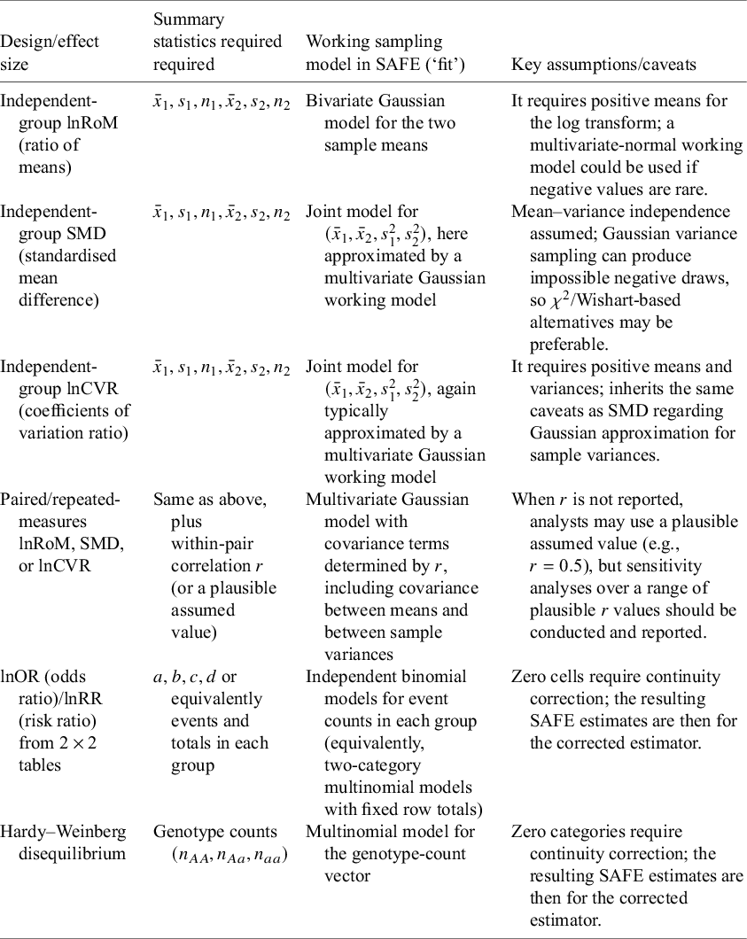
Table 1 summarises the settings for the effect sizes above, the summary statistics required, the working sampling models used, and the main caveats. In all cases, SAFE proceeds by specifying a working model for the reported summary statistics, drawing bootstrap replicates under that model, transforming each replicate into the effect size of interest, and then summarising the resulting bootstrap cloud. What differs across designs is the choice of sampling model and the assumptions needed to justify it. Notably, the SAFE implementations presented above are most appropriate for effect sizes that can be expressed on an approximately unbounded, reasonably symmetric scale and parameterised from commonly reported descriptive statistics; SAFE should not be applied to highly skewed or bounded raw effect sizes without adopting a more appropriate sampling model.
Practical notes for applying SAFE to the effect sizes covered in this tutorial

Table 1 Long description
The table consists of four columns: Design/effect size, Summary statistics required, Working sampling model in S A F E (‘fit’), and Key assumptions/caveats.
* Row 1: Independent-group ln R o M (ratio of means). Statistics: x-bar sub 1, s sub 1, n sub 1, x-bar sub 2, s sub 2, n sub 2. Model: Bivariate Gaussian model for the two sample means. Caveats: Requires positive means for log transform.
* Row 2: Independent-group S M D (standardised mean difference). Statistics: x-bar sub 1, s sub 1, n sub 1, x-bar sub 2, s sub 2, n sub 2. Model: Joint model for (x-bar sub 1, x-bar sub 2, s sub 1 squared, s sub 2 squared), approximated by a multivariate Gaussian model. Caveats: Mean-variance independence assumed; chi-squared/Wishart alternatives may be preferable to avoid negative draws.
* Row 3: Independent-group ln C V R (coefficients of variation ratio). Statistics: x-bar sub 1, s sub 1, n sub 1, x-bar sub 2, s sub 2, n sub 2. Model: Joint model for (x-bar sub 1, x-bar sub 2, s sub 1 squared, s sub 2 squared). Caveats: Requires positive means and variances.
* Row 4: Paired/repeated-measures ln R o M, S M D, or ln C V R. Statistics: Same as above plus within-pair correlation r. Model: Multivariate Gaussian model with covariance terms determined by r. Caveats: If r is not reported, use a plausible value like r = 0.5 and conduct sensitivity analyses.
* Row 5: ln O R (odds ratio)/ln R R (risk ratio) from 2 times 2 tables. Statistics: a, b, c, d or events and totals. Model: Independent binomial models for event counts. Caveats: Zero cells require continuity correction.
* Row 6: Hardy-Weinberg disequilibrium. Statistics: Genotype counts (n sub A A, n sub A a, n sub a a). Model: Multinomial model for the genotype-count vector. Caveats: Zero categories require continuity correction.
Note: The table summarises the required reported summaries, the working sampling model used in the SAFE ‘fit’ step, and the key assumptions or caveats for each setting.
Important, so far, every example has focused on computing an effect size for single comparison, chiefly to make the four SAFE steps clear. In reality, however, meta-analyses, comprise multiple pairwise comparisons (e.g., means, SD, and
$n$
 ). Fortunately, our procedure parallelises naturally. In R for example, we can wrap the SAFE function in mapply() or, pmap() from the purrr package,Reference Wickham and Henry
31
which dispatches the function row-wise and binds the results in to a single data frame (parallelised functions are available for the effect sizes introduced above as part of an additional material: https://ejlundgren.github.io/SAFE/).
The R script below illustrates the workflow for log response ratios (ratio of means; safe_RoM) using a meta-analytic dataset from Curtis and Wang,Reference Curtis and Wang 32 which is a part of the metadat package.Reference Viechtbauer, White, Noble, Senior and Hamilton 33 As shown below, one instance of mapply() returns two named columns (y_SAFE and v_SAFE), respectively, containing the SAFE point estimates and variances for each pairwise set of summary statistics. Note that, for comparison, we also have point estimates and variances (yi, vi) obtained via escalc() from the metafor package.Reference Viechtbauer 22
## ---- 0.  preparations  -------------------------------------------------
library(metafor)
library(metadat)
set.seed(777)

## ---- 1.  SAFE log response ratios  -------------------------------------
# dataset and sampling data row indices
dat1 <- dat.curtis1998[sample(nrow(dat.curtis1998), 10), c(1, 15:20)]

# functions for lnRoM
safe_RoM <- function(x1, x2, s1, s2, n1, n2, B = 1e6) {
  # plug-in estimate
  t0 <- log(x1/x2)
  # draws
  x1_star <- rnorm(B, mean = x1, sd = s1/sqrt(n1))
  x2_star <- rnorm(B, mean = x2, sd = s2/sqrt(n2))
  # transform, drop any non-positive draws (if any)
  ts <- log(x1_star[x1_star>0 & x2_star>0] / x2_star[x1_star>0 & x2_star>0])
  # bias, bias-corrected point estimate and variance
  c(y_SAFE  = 2*t0 - mean(ts),
    v_SAFE  = var(ts)
    )
}

dat1 <- escalc(measure = "ROM",
               m1i = dat1$m1i, sd1i = dat1$sd1i, n1i = dat1$n1i,
               m2i = dat1$m2i, sd2i = dat1$sd2i, n2i = dat1$n2i,
               data = dat1, append = TRUE)

safe_out1 <- mapply(  safe_RoM,
  x1 = dat1$m1, x2 = dat1$m2,           # means
  s1 = dat1$sd1, s2 = dat1$sd2,         # SDs
  n1 = dat1$n1,  n2 = dat1$n2,          # sample sizes
  SIMPLIFY = TRUE)

# round for easy comparisons, but usually not recommended
dat1$yi_SAFE <- round(safe_out1["y_SAFE", ], 4)
dat1$vi_SAFE <- round(safe_out1["v_SAFE", ], 4)
If you run this script, we will get the following:
> dat1
    id      m1i       sd1i n1i     m2i      sd2i n2i     yi     vi yi_SAFE vi_SAFE
24 242   2.2000   0.411100  10   1.330  0.189700  10 0.5033 0.0055  0.5041  0.0056
1   21   6.8169   1.769982   3   3.945  1.115797   5 0.5470 0.0385  0.5503  0.0406
90 739  16.5900   2.914900   6  13.800  1.592200   6 0.1841 0.0074  0.1856  0.0074
60 456  38.3600   3.215000   2  26.490  1.790000   2 0.3702 0.0058  0.3708  0.0058
62 458 186.2600  11.834000   2 180.480 11.867000   2 0.0315 0.0042  0.0314  0.0042
83 726  16.9800   1.959600   6  10.960  1.935100   6 0.4378 0.0074  0.4362  0.0075
12  96  72.5000  15.000000  24  60.500 14.000000  24 0.1809 0.0040  0.1807  0.0040
10  87  71.7200  14.300000  16  59.940 14.280000  16 0.1794 0.0060  0.1788  0.0061
76 615 374.4000 109.567300   5 298.200 96.374500   5 0.2276 0.0380  0.2258  0.0400
25 254  23.1100   0.844300  22  14.940  0.844300  22 0.4362 0.0002  0.4362  0.0002
The same process can be implemented using the log risk ratio (lnRR; safe_RR), with the dataset from Graves et al.,Reference Graves, Deeks, Demicheli and Jefferson 34 which is also part of the metdat package.
## ---- 2.  SAFE log risk ratios  -------------------------------------
# dataset and sampling data row indices (note should be dat.graves1996)
dat2 <- dat.graves2010[sample(nrow(dat.graves2010), 10), ]

# function for lnRR ---------------------------------------------------
# note the function is slightly different from the above
# (it takes n1 and n2 rather than b and d
safe_RR <- function(a, c, n1, n2, B   = 1e6,
                       add = 0.5) { # continuity correction

  ## continuity correction --------------------------------------------
  add1 <- if (a == 0) add else 0          # only if the observed cell is zero
  add2 <- if (c == 0) add else 0
  # note the +add on *both* successes & failures
  p1_hat <- (a + add1) / (n1 + add1*2)
  p2_hat <- (c + add2) / (n2 + add2*2)
  lnRR_raw <- log(p1_hat / p2_hat)
  # draw once
  a_star <- rbinom(B, n1, a / n1)
  c_star <- rbinom(B, n2, c / n2)
  # transform
  add1_star <- ifelse(a_star == 0, add, 0)
  add2_star <- ifelse(c_star == 0, add, 0)
  p1_star <- (a_star + add1_star) / (n1 + add1_star*2)
  p2_star <- (c_star + add2_star) / (n2 + add2_star*2)
  lnRR_star <- log(p1_star / p2_star)
  # bias, bias-corrected point estimate and variance
  c(y_SAFE  = 2*lnRR_raw - mean(lnRR_star),
    v_SAFE  = var(lnRR_star)
  )
}

dat2 <- escalc(measure = "RR",
               ai = dat2$ai, ci = dat2$ci,        # events in ctrl/treat
               n1i = dat2$n1i, n2i = dat2$n2i,
               data = dat2,
               add = 0.5, to = "only0", append = TRUE)

safe_out2 <- mapply(  safe_RR,
  a  = dat2$ai, n1 = dat2$n1,           # events + totals (grp1)
  c  = dat2$ci, n2 = dat2$n2,           # events + totals (grp2)
  SIMPLIFY = TRUE)

# round for easy comparisons, but usually not recommended
dat2$yi_SAFE <- round(safe_out2["y_SAFE", ], 4)
dat2$vi_SAFE <- round(safe_out2["v_SAFE", ], 4)
We should now get this data frame.
> dat2
             study ai    n1i ci   n2i      yi     vi yi_SAFE vi_SAFE
12  Azurin 1965-ii 92 148100 52 48933 -0.5369 0.0301 -0.5410  0.0308
16   Saroso 1978-i 18 156300 19 79250 -0.7332 0.1082 -0.7316  0.1186
9    PCC 1973a-iii 36  44450 23 11050 -0.9439 0.0711 -0.9527  0.0756
8     PCC 1973a-ii 33  45750 22 11050 -1.0153 0.0756 -1.0233  0.0806
3    Mosley 1970-i 32  11491 13  3810 -0.2031 0.1078 -0.2286  0.1205
17  Saroso 1978-ii 10 155600 18 79250 -1.2625 0.1555 -1.2367  0.1819
1    Oseasohn 1965  8   6956 33  7103 -1.3962 0.1550 -1.3413  0.1911
15        PCC 1968 54 268700 41 90900 -0.8084 0.0429 -0.8116  0.0443
10    PCC 1973a-iv 26  44700 22 11050 -1.2305 0.0838 -1.2341  0.0896
13 Azurin 1965-iii 71 143600 52 48933 -0.7651 0.0333 -0.7679  0.0342
As you can see, SAFE provides very similar point estimates and variance estimates as escalc(), though the variance estimates are often larger (more conservative), and this discrepancy disappears as the sample size grows. In practice, for many existing studies, SAFE may not change the qualitative conclusions. However, the SAFE procedure future-proofs the analysis for new effect-size statistics. Additionally, one can compare the point estimate and variance derived from the delta method for new effect size statistics with those obtained using the SAFE bootstrap, as we have done in this tutorial.
7. Concluding remarks
In this tutorial, we have introduced the SAFE bootstrap that builds on previous single-fit parametric methods.Reference Mandel 6 , Reference Fletcher and Jowett 7 SAFE bootstrap provides a practical and transparent model-based route to bias correction and SE estimation when only summary statistics are available. By following the four-step recipe (fit, draw, transform, and summarise), researchers can avoid deriving a new delta-method formula for every new effect size, while making the assumed sampling model explicit. This approach lowers the barrier to obtaining model-based BC point estimates and SEs for many effect sizes that can be expressed as functions of reported summary statistics, provided an appropriate sampling model can be specified. Although this is not the focus of our article, our simulation validation suggests that in the settings considered here, SAFE point estimates could outperform plug-in and small-sample-corrected formulas, especially when sample sizes are small. In line with our results, the simulation work of Fletcher and JowettReference Fletcher and Jowett 7 demonstrated that confidence intervals (CIs) derived from the SAFE procedure (i.e., single-fit bootstrapping) outperformed those obtained using the delta method, suggesting that single-fit bootstrap procedures can outperform delta-method-based CIs in some settings. Yet, we also note that delta-method-based variance estimators could outperform their SAFE counterparts in some scenarios; SAFE sampling variance tends to be higher than that of the delta method (see an additional material: https://ejlundgren.github.io/SAFE/).
Here, we have also shown that the SAFE procedure can be applied to familiar effect size statistics, such as lnRoM, SMD, lnOR, and lnRR. Yet the true potential of the SAFE bootstrap lies in its adaptability. The same reasoning and coding pipeline can be applied to less common but valuable metrics, such as lnCVRReference Nakagawa, Poulin and Mengersen 8 , Reference Senior, Viechtbauer and Nakagawa 9 or the HWE statistic,Reference Wellek, Goddard and Ziegler 10 as illustrated. Additionally, for some effect sizes, variance estimators are not derived for paired or dependent designs; however, this is not an issue for the SAFE approach, which can readily handle dependence. This flexibility allows researchers to choose the most suitable effect size for their specific question, rather than being restricted to effect sizes for which estimators of the sampling variance exist.
A natural next step will be to consider whether SAFE can be extended beyond the two-group designs treated here, for example, to sample correlations,
$R^2$
 , regression coefficients, or more complex effect sizes arising from longitudinal, covariate-adjusted, or multilevel models. However, these extensions are not straightforward. In many such settings, the primary study already reports SEs for the target estimate, so SAFE would mainly be useful when one wishes to transform the estimate or construct a more complex derived effect size. Relatedly, SAFE might be useful for converting effect size statistics; correlation, lnOR, and SMD are convertible to each other,Reference Borenstein, Hedges, Higgins and Rothstein
18
but these formulas are likely to introduce bias due to their non-linear nature. It is also an interesting avenue for future research to apply the SAFE procedure to the concept of ‘smooth variance estimators’, in which sampling variance is calculated by averaging observed parameter values. For example, this approach can be applied to CV, which is a part of the sampling variance formula for lnRoM, improving the estimation of overall (meta-analytic) means.Reference Nakagawa, Noble, Lagisz, Spake, Viechtbauer and Senior
35
With SAFE, the initial ‘fit’ step is the crucial one, because it requires choosing a sampling model for the reported statistics. In this tutorial, we have made heavy use of Gaussian working models for continuous outcomes and binomial or multinomial models for discrete outcomes, as these are often parameterisable from the summary information reported in primary studies. However, SAFE does not remove the need for statistical judgement: if the working model is poor, the resulting bias correction and SE may also be poor. In principle, one could instead use positive-support models, such as log-normal or gamma models for some continuous outcomes, but these often require additional assumptions or parameterisation choices that are not identifiable from the usual reported summaries alone.Reference Higgins, White and Anzures-Cabrera 36 Extending SAFE to such settings remains an important direction for future work. Heuristically, the SAFE bootstrap cloud can resemble the way one works with a Bayesian posterior distribution, in the sense that inference is based on a simulated distribution of the quantity of interest rather than a closed-form approximation.Reference Efron 37
Notably, traditional bootstrap procedures applied directly to raw data remain an important benchmark.Reference Efron 1 – Reference Davison and Hinkley 4 When raw data are available, or if a primary study already reports bootstrap-based effect-size estimates and corresponding SEs or confidence intervals derived from the raw data, those should generally be preferred. SAFE is designed for the more typical meta-analytic situation in which only summary statistics are available. Accordingly, SAFE is most useful when raw data are unavailable and one needs a transparent, model-based way to obtain BC effect-size estimates and SEs from reported summaries, especially when sampling variance formulas are unavailable, difficult to derive, or potentially inaccurate in small samples. However, SAFE is not assumption-free: it should only be used when the analyst can specify a plausible working model for the sampling distribution of the reported statistics.
Ultimately, we believe the SAFE bootstrap offers a useful addition to the meta-analyst’s toolkit. We do not propose SAFE as a replacement for elegant analytic formulas or for raw-data bootstrap procedures when those are available. Rather, SAFE fills an important practical gap: it offers a computationally efficient, transparent, and reproducible summary-statistic approach when raw data are unavailable and when analytic variance formulas are unavailable, difficult to derive, or potentially inaccurate in small samples. In that role, SAFE can both support applied work and help researchers build a deeper intuition for sampling distributions, transformation-induced bias, and simulation-based inference.Reference Noble, Radersma and Uller 38 – Reference Nakagawa, Mizuno and Williams 41 Therefore, the path to more accessible meta-analytic inference is, as we have shown, a SAFE one.
Acknowledgements
S.N. acknowledges that conversations with David Fletcher and Wolfgang Viechtbauer have inspired the idea of this manuscript, and S.N. would like to thank them.
Author contributions
Conceptualization: S.N., A.M., C.W., S.O., S.D., M.L., Y.Y., A.S., D.W.A.N., and E.L.; Formal analysis: E.L. and S.N.; Funding acquisition: S.N. and M.L.; Investigation: E.L. and S.N.; Methodology: E.L. and S.N.; Project administration and supervision: S.N.; Validation: E.L., D.W.A.N., A.M.S. and S.O.; Visualisation: A.M.; Writing—original draft: S.N. and E.L.; Writing—review and editing: S.N., A.M., C.W., S.O., S.D., M.L., Y.Y., A.S., D.W.A.N., and E.L.
Competing interests
The authors declare no competing interests.
Data availability statement
All data and code are available at the GitHub repository: (https://github.com/ejlundgren/SAFE). They are also archived at the Zenodo repository: (https://zenodo.org/records/20637924).
Funding statement
S.N., S.O., A.M., and E.L. were supported by the Canada Excellence Research Chair Program (CERC-2022-00074). Y.Y., M.L., and S.N. were supported by the Australian Research Council Discovery Project (DP230101248). A.S. and D.W.A.N. were supported by an Australian Research Council Future Fellowship (FT230100240 and FT220100276, respectively). S.M.D. was supported by the Polish National Science Center OPUS grant (no. UMO-2024/55/B/NZ8/02816).
AI use statement
The authors used AI tools in a limited and supportive capacity during the preparation of this manuscript, specifically to check the simulation code and to improve the clarity and flow of the writing during editing. These tools were not used to generate scientific conclusions. All analyses, interpretations, and final text were reviewed, verified, and approved by the authors, who take full responsibility for the content of the article.



 Open access

