3.1 From spectral to topological torsion series

We start with the proof of the first identity $\vartheta = \vartheta ^{top}$ . Recall that by Lefschetz decomposition (17)

$$ \begin{align*} \Omega^* H = \bigoplus_{0\leq p \leq q \leq n} L^p \mathcal{E}^{n-q} \,. \end{align*} $$

Therefore $\Omega ^*H$ contains $n+1-k$ copies of each $\mathcal {E}^k$ for $0\leq k\leq n$ . This is the multiplicity of $\mathcal {E}^k$ in $\vartheta $ . Moreover, since $L= d\theta \wedge \cdot $ preserves the parity, the parity of forms in $\Omega ^*H$ and their components in $\mathcal {E}^*$ coincides. Thus the plus and minus parts of $\vartheta $ combine to give

$$ \begin{align*} \vartheta(t) = \operatorname{\mathrm{Tr}} (e^{-t \boldsymbol{\Delta}_Q} \mid \Omega^{ev} H) - \operatorname{\mathrm{Tr}} (e^{-t \boldsymbol{\Delta}_Q} \mid \Omega^{odd} H) \,. \end{align*} $$

Now $D_H = d_H + \delta _H$ exchanges $\Omega ^{ev}H$ and $\Omega ^{odd}H$ and commutes with $\boldsymbol {\Delta }_Q$ by Section 2.3. Hence, setting $\mathcal {H}= \ker D_H$ , one has

$$ \begin{align*} \vartheta(t) = \operatorname{\mathrm{Tr}} (e^{-t \boldsymbol{\Delta}_Q} \mid \mathcal{H}^{ev}) - \operatorname{\mathrm{Tr}} (e^{-t \boldsymbol{\Delta}_Q} \mid \mathcal{H}^{odd}) \,. \end{align*} $$

We need the following lemma to identify the residual spectrum on $\mathcal {H}$ .

Note that $\mathcal {H}=\ker D_H$ should not be confused with $\ker \Delta _H=\ker d_H \cap \ker \delta _H$ since $d_H$ is not a complex by (13). The next proposition will lead us to a useful description of $\mathcal {H}$ .

Proposition 3.4. Let $P=L+\Lambda $ acting on $\Omega ^*H$ and $U= e^{i\pi P/4}$ . Then on a contact manifold with an integrable J, it holds that

$$ \begin{align*} \left\{ \begin{aligned} [P,D_H]& = d_H^J - \delta_H^J \\ [P,d_H^J -\delta_H^J] & = D_H \end{aligned} \right. \end{align*} $$

and

$$ \begin{align*} U^{-1}D_H U = \sqrt2 (\overline\partial_H + \overline\partial_H^*)\,. \end{align*} $$

Proof. The first identities come from (13) and (18) giving $[L,d_H]= 0$ and $[\Lambda ,d_H]=-\delta _H^J$ and conjugate relations. Therefore for any angle $\varphi $

$$ \begin{align*} e^{i\varphi\, \mathrm{ad}(P)} D_H &= \cos \varphi D_H + i \sin \varphi (d_H^J-\delta_H^J) \\ & = \mathrm{Ad}(e^{i\varphi P}) D_H = e^{i\varphi P} D_H e^{-i\varphi P} \,. \end{align*} $$

This yields the last identity using $\varphi = -\pi /4$ and the splitting of $d_H = \partial _H + \overline \partial _H$ for integrable J by (24).

Let $\mathcal {H}_{\overline \partial _H}=\ker (\overline \partial _H + \overline \partial _H^*)$ . By the previous proposition

$$ \begin{align*} \mathcal{H}= \ker D_H = U (\mathcal{H}_{\overline\partial_H})\,, \end{align*} $$

with the advantage that on CR Seifert manifolds $\overline \partial _H^2=0$ from (13). Hence one has also $\mathcal {H}_{\overline \partial _H}= \ker \Delta _{\overline \partial _H}$ with

$$ \begin{align*} \Delta_{\overline\partial_H} = \overline\partial_H \overline\partial_H^* + \overline\partial_H^* \overline\partial_H \,. \end{align*} $$

Now by definition $\Delta _{\overline \partial _H}$ preserves the bidegree of forms, but also the spaces $L^k \Omega ^p_0H$ in the Lefschetz decomposition. This is due to the commutation relation

$$ \begin{align*} \Delta_{\overline\partial_H}L = L(\Delta_{\overline\partial_H} -i T) \end{align*} $$

that comes from (18) when $\mathcal {L}_T J=0$ . Indeed, from

$$ \begin{align*} [L, \overline\partial_H] = 0 \quad \mathrm{and} \quad [L, \overline\partial_H^*]= -i \partial_H \end{align*} $$

one gets

$$ \begin{align*} \Delta_{\overline\partial_H}L - L\Delta_{\overline\partial_H} = i (\partial_H \overline \partial_H + \overline\partial_H \partial_H) = -iL T \end{align*} $$

by (13). This leads eventually to the splitting of $\mathcal {H}_{\overline \partial _H}$ into forms of pure bidegree and type in the Lefschetz decomposition. Using (19) we first find:

Proposition 3.5. On a CR Seifert manifold, one has

$$ \begin{align*} \ker \overline\partial_H = \begin{cases} \ker \overline\partial_Q \cap \ker \partial_Q^* & \quad \mathrm{on}\ L^k \mathcal{E}^{n-q} \ \mathrm{for}\ 0\leq k< q\leq n\\ \ker \partial_Q^* & \quad \mathrm{on} \ L^q \mathcal{E}^{n-q} \end{cases} \end{align*} $$

and

$$ \begin{align*} \ker \overline\partial_H^* = \begin{cases} \ker \overline\partial_Q^* \cap \ker \partial_Q & \quad \mathrm{on}\ L^k \mathcal{E}^{n-q} \ \mathrm{for}\ 1 \leq k\leq q \leq n\\ \ker \overline\partial_Q^* & \quad \mathrm{on} \ \mathcal{E}^{p} \ \mathrm{for} \ 0\leq p\leq n\,. \end{cases} \end{align*} $$

In conclusion

$$ \begin{align*} \mathcal{H}_{\overline\partial_H} = \begin{cases} \ker \Delta_Q & \quad \mathrm{on} \ L^k\mathcal{E}^{n-q} \ \mathrm{for}\ 1\leq k< q \leq n\\ \ker \overline\partial_Q \cap \ker \partial_Q^* \cap \ker \overline\partial_Q^* & \quad \mathrm{on}\ \mathcal{E}^p \ \mathrm{for}\ p< n\\ \ker \partial_Q^* \cap \ker \overline\partial_Q^* \cap \ker \partial_Q & \quad \mathrm{on} \ L^q \mathcal{E}^{n-q}\ \mathrm{for}\ 0 < q \leq n\\ \ker \partial_Q^* \cap \ker \overline\partial_Q^* & \quad \mathrm{on} \ \mathcal{E}^n \,. \end{cases} \end{align*} $$

This leads to the following results on $\mathcal {H}_{\overline \partial _H}$ :

• • On $L^k \mathcal {E}^{n-q}$ for $0\leq k < q \leq n$ , $\Delta _Q=\Delta _Q^J=\mathcal {L}_T=0$ by (27),

• • On $\mathcal {E}^p$ for $p<n$ , $\Delta _{\overline \partial _Q}=0$ , so that by (27) $\Delta _Q = -i T$ and $\boldsymbol {\Delta }_Q = \Delta _Q^2 = - T^2$ ,

• • On $L^q\mathcal {E}^{n-q}$ for $0< q \leq n$ , $\Delta _{\partial _Q} =0$ , so that $\Delta _Q = i T$ and $\boldsymbol {\Delta }_Q = \Delta _Q^2 = -T^2$ ,

• • On $\mathcal {E}^n$ , $\delta _Q=0= \delta _Q^J=0$ , so that $i_TD = T$ and $\boldsymbol {\Delta }_Q = - T^2$ .

This yields Lemma 3.3 because the isometry $U = e^{i \frac {\pi }{4} (L+\Lambda )}$ mapping $\mathcal {H}_{\overline \partial _H}$ to $\mathcal {H}=\ker D_H$ in Proposition 3.4 commutes with $\boldsymbol {\Delta }_Q$ and T, hence preserves the equation $\boldsymbol {\Delta }_Q = -T^2$ .

To conclude with this study of $\mathcal {H}$ we observe that it is infinite dimensional since it contains images by U of CR functions (satisfying $ \overline \partial _H f=0$ ).

We have obtained that

(30) $$ \begin{align} \vartheta(t) = \operatorname{\mathrm{Tr}}(e^{tT^2} \mid \mathcal{H}^{ev}) - \operatorname{\mathrm{Tr}}(e^{tT^2 } \mid \mathcal{H}^{odd}) \,. \end{align} $$

Note that both traces converge since they are parts of traces of the heat operators $e^{-t \boldsymbol {\Delta }_Q}$ . The next step will be to split this as a series of indices using a twisted Fourier decomposition along the circle action by T. We discuss this briefly and refer to [Reference Rumin and Seshadri20, Section 4.1] for a more detailed discussion. We will suppose that M is connected in the sequel of this section. The general case reduces to it by summing the contributions of each connected component.

The flat bundle V over M associated to the unitary representation $\rho : \pi _1(M) \rightarrow U(d)$ is the quotient of the trivial bundle $\widetilde M \times \mathbb C^d$ by the deck transformations $\gamma .(m,v) = (\tau (\gamma )m, \rho (\gamma ) v)$ . The circle action $\varphi _t$ induced by T on M may be lifted to V by parallel transport using the flat connection $\nabla ^\rho $ . On V we don’t have a circle action since

$$ \begin{align*} \varphi_{2\pi} = \rho(f)^{-1} \end{align*} $$

where $f= \varphi _{[0,2\pi ]}(m)$ is a generic closed primitive orbit. However, over each connected component of M, we can split V into bundles $V^x$ on which

$$ \begin{align*} \rho(f) = e^{2i \pi x} \end{align*} $$

with $x \in ]0,1]$ by convention. Note that the bundles $V^x$ are flat since the homotopy class of f lies in the center of $\pi ^1(M)$ as seen using the flow. We recover a circle action on $V^x$ by setting

$$ \begin{align*} \psi_t = e^{i t x} \varphi_t \,. \end{align*} $$

We can still perform a Fourier decomposition of sections $s \in \mathbf {V}^x = \Gamma (M, V^x)$ . One has

$$ \begin{align*} s = \sum_{n\in \mathbb Z} \pi_n s \quad \mathrm{with} \quad \pi_n s = \frac{1}{2\pi} \int_0^{2\pi } e^{-int } \psi_t(s) dt \,. \end{align*} $$

Since $\psi _t(\pi _ns) = e^{int} \pi _n s$ one gets that $\nabla ^\rho _T(\pi _ns) = i(n-x) \pi _ns$ and the spectrum of $iT= i\nabla ^\rho _T $ on $\mathbf {V}^x$ is the shifted $x+\mathbb Z$ . For $\lambda = x+n$ we shall note

(31) $$ \begin{align} \mathbf{V}_{\lambda} = \pi_{-n} (\mathbf{V}^x) = \mathbf{V}^x \cap \{ iT = \lambda\}. \end{align} $$

Since T commutes with all our geometric operators including $D_H$ , we can split the V-valued bundle

$$ \begin{align*} \mathcal{H}= \ker D_H = \bigoplus_{\lambda \in \operatorname{\mathrm{Spec}}(iT)} \mathcal{H} \cap \mathbf{V}_\lambda \,. \end{align*} $$

Therefore (30) eventually reads

$$ \begin{align*} \vartheta(t) & = \sum_{\lambda \in \operatorname{\mathrm{Spec}}(iT)} \big(\dim(\mathcal{H}^{ev} \cap \mathbf{V}_\lambda )- \dim(\mathcal{H}^{odd} \cap \mathbf{V}_\lambda) \big) e^{-t \lambda^2} \\ & = \sum_{\lambda \in \operatorname{\mathrm{Spec}} (iT)} \operatorname{\mathrm{ind}} (D_H^{ev} \mid \mathbf{V}_\lambda) e^{-t \lambda^2} = \vartheta^{top}(t) \,, \end{align*} $$

with $D_H^{ev} : \Omega ^{ev}H \rightarrow \Omega ^{odd}H$ . This is the topological version of the $\vartheta $ series. We shall see that these indices can be interpreted as coming from operators and bundles over the orbifold $N = M/\mathbf {S}^1$ .

3.2 Orbifold structure and index computations.

These indices in the previous formula can be computed using the index theorem for V-(orbi)bundles over V-manifolds (orbifolds) as developed by Kawasaki in [Reference Kawasaki14]. One first has to interpret the index of $D_H^{ev}$ on $\mathbf {V}_\lambda $ as the index of an operator over the orbifold $N = M /\mathbf {S}^1$ acting on a V-bundle.

We follow the discussion in [Reference Rumin and Seshadri20, section 5.2]. We first introduce the relevant V-(orbi)bundle here. Given a point $p \in N$ , we consider the vector space $V_\lambda (p)$ of sections of $V^x$ along the orbit $\mathbf {S}^1(p)$ in M satisfying $iT s = \lambda s$ . Call $V_\lambda $ this family of spaces. One has by definition

$$ \begin{align*} \mathbf{V}_\lambda = \Gamma(N, V_\lambda) \,, \end{align*} $$

and $V_\lambda $ is a vector bundle of dimension $\dim V^x$ over the generic non-singular points of N since the circle action is free there.

We now describe the orbifold structure of $V_\lambda $ near a singular point $p_j$ corresponding to an exceptional closed primitive orbit $f_j$ of order $\alpha _j$ . That means that the isotopic group of the circle action on $f_j$ is the cyclic group of order $\alpha _j$ . From the Slice Theorem, locally over $p_j$ the bundle $V^x$ is isomorphic to the quotient of the trivial bundle $\mathbb C^n \times \mathbb R \times \mathbb C^{\dim V^x}$ by the deck transformation

(32) $$ \begin{align} F_j : (p,t,v) \mapsto (M_j(p), t + 2\pi / \alpha_j, \rho(f_j) v) \end{align} $$

where $M_j(p) \in U(n)$ generates a cyclic group of order $\alpha _j$ . Now let $\widetilde V_\lambda $ be the trivial bundle over $\mathbb C^n$ whose fibre over p consists of functions $s_p : \mathbb R \rightarrow \mathbb C^{\dim V_x}$ satisfying $s_p(t) = e^{-i\lambda t} s_p(0)$ . Since $(iT) s_p = \lambda s_p$ , one sees that a section $s : p \mapsto s_p$ of $\widetilde V_\lambda $ near $0\in \mathbb C^n$ descends to $\mathbf {V}_\lambda $ if it is invariant under the deck transformation $F_j$ above. This means that $(p, s_p(0))$ is invariant by

(33) $$ \begin{align} F_{j,\lambda} : (p, v) \mapsto (M_j(p) , e^{-2i \pi \lambda / \alpha_j} \rho(f_j)v) \,. \end{align} $$

Since $f_j^{\alpha _j} \sim f$ in $\pi _1(M)$ , one has $\rho (f_j)^{\alpha _j} = \rho (f) = e^{2i\pi x}$ and $F_{j,\lambda }^{\alpha _j} = \operatorname {\mathrm {id}}$ .

This shows that $V_\lambda $ is a V-bundle (orbi-bundle) over N since locally over $p_j$ it is the quotient of $\widetilde V_\lambda $ by the finite group $\Gamma _j \simeq \mathbb Z/\alpha _j \mathbb Z$ generated by $F_{j,\lambda }$ .

At this point we can identify $\mathrm {ind}(D_H^{ev} \mid \mathbf {V}_\lambda )$ as being the index of the Dirac operator $D_H^{ev}$ acting on sections of the V-bundle $V_\lambda $ over N. Note that even though $d_H$ is not a complex, the operator $D_H$ is elliptic on N as $D_H^2 = \Delta _H -L T + T\Lambda = \Delta _H$ up to order- $0$ terms on $V_\lambda $ . More concretely from Proposition 3.4, $D_H$ is unitarily conjugated to ${\partial\mskip-10mu/ }_H = \overline \partial _H + \overline \partial _H^*$ , hence

$$ \begin{align*} \operatorname{\mathrm{ind}}(D_H^{ev} \mid V_\lambda) & = \operatorname{\mathrm{ind}}({\partial\mskip-10mu/ }_H \mid \Omega^{ev}H \otimes V_\lambda) \\ & = \sum_p (-1)^p \chi_{\overline\partial_H} (N,\Omega^{p,0}H \otimes V_\lambda) \end{align*} $$

where $\chi _{\overline \partial _H}(N,\Omega ^{p,0}H \otimes V_\lambda )$ is the holomorphic Euler characteristic of the V-bundle $\Omega ^{p,0}H \otimes V_\lambda $ . Recall that $\overline \partial _H^2 =0$ on CR Seifert manifolds by (13). From this discussion, one can compute these indices using Kawasaki’s Riemann–Roch theorem for complex V-manifolds [Reference Kawasaki14]. It reads here

(34) $$ \begin{align} \operatorname{\mathrm{ind}}(D_H^{ev} \mid V_\lambda) = \langle \operatorname{\mathrm{ch}} (V_\lambda) \wedge e (N)_{orb} , [N] \rangle_{orb} \,. \end{align} $$

This pairing on the orbifold N splits into a usual smooth contribution over the generic orbits of the characteristic classes and an average of equivariant classes over components of exceptional orbits in various singular strata; see [Reference Kawasaki14, Reference Atiyah and Bott3]. To be more explicit, we need first to discuss the stratification of N.

The orbifold N splits into the connected components $N_j$ of its strata that are determined by the possible isotopy groups $\Gamma \simeq \mathbb Z/\alpha Z$ of the circle action. We note $N = \bigsqcup _{j \in \mathcal {S}} N_j$ this decomposition and $\alpha _j$ the order of the isotopy group in $N_j$ . Then pick one primitive orbit $f_j$ in each $N_j$ . By (32), one has locally around $f_j$ that N identifies with the quotient of $\mathbb C^n$ by a cyclic group of order $\alpha _j$ generated by a unitary ‘isotopy’ matrix $M_j$ . Let

$$ \begin{align*} \sigma_j= \mathrm{Spec}(M_j) \end{align*} $$

be its spectrum. It consists of $\alpha _j$ -th roots of unity. Let $d_\lambda $ denote the order of $\lambda \in \sigma _j$ . It divides $\alpha _j$ and the least common multiple of these $d_\lambda $ is $\alpha _j$ .

Locally the stratum $N_j$ containing $f_j$ is given by $\ker (M_j - \operatorname {\mathrm {id}})$ . Other strata $N_k$ around $f_j$ are given by the sets of points of order exactly d in

(35) $$ \begin{align} \ker(M_j^d - \operatorname{\mathrm{id}})= \bigoplus_{\{\lambda \in \sigma_j,\ d_\lambda \mid d\}} \ker (M_j - \lambda \operatorname{\mathrm{id}}) \,, \end{align} $$

for some divisors d of $\alpha _j$ , when these sets are non empty. This happens when d is the least common multiple of $\{\lambda \in \sigma _j, \ d_\lambda \mid d\}$ . In these cases $f_k \in N_k$ is homotopic to $f_j^d$ . Note that from this local model, the set $\mathcal {S}$ labelling the connected components of strata is finite on the compact N. Moreover the closure of a stratum consists of the union of the connected components of strata it contains.

Using this orbifold structure, the action of the isotopy group on $V_\lambda $ given in (33) and Kawasaki’s formula, one finds that (34) gives here

(36) $$ \begin{align} \operatorname{\mathrm{ind}}(D_H^{ev} \mid V_\lambda) = \sum_{j \in \mathcal{S}} \frac{1}{\alpha_j} \sum_{k \in K_j \cap [0 \, .. \,\alpha_j-1]} e^{-2 i \pi k \lambda / \alpha_j} \chi_\rho(f_j^k) \int_{N_j}e(TN_j) \nu(f_j^k) \,, \end{align} $$

where

$$ \begin{align*} K_j = \{k \in \mathbb Z \textrm{ such that } \ker (M_j^k -\operatorname{\mathrm{id}})= \ker (M_j - \operatorname{\mathrm{id}}) \}\,, \end{align*} $$

$e(TN_j)$ is the Euler class of $N_j$ and $\nu (f_j^k)$ is the Lefschetz index of the Poincaré return map along $f_j^k$ acting on the normal bundle of $N_j$ . Since $df_j^k \in U(n)$ , one has $\nu (f_j^k)= 1$ here so that (36) reduces to

(37) $$ \begin{align} \operatorname{\mathrm{ind}}(D_H^{ev} \mid V_\lambda) = \sum_{j \in \mathcal{S}} \frac{\chi^{orb}(N_j)}{\alpha_j} \sum_{k \in K_j \cap [0 \, .. \, \alpha_j-1]} e^{-2 i \pi k \lambda / \alpha_j} \chi_\rho(f_j^k) \,, \end{align} $$

where $\chi ^{orb}(N_j) = \int _{N_j} e(TN_j)$ is the rational (orbifold) Euler characteristic of $N_j$ . Note that in this sum, the case $k=0$ only appears for $\alpha _j=1$ and corresponds to the contribution of the generic regular orbits.

Our next step is to express this sum using integral data from N and $\rho $ . We shall prove the following.

Proposition 3.6. Let M be a connected CR Seifert manifold. Then

$$ \begin{align*} \operatorname{\mathrm{ind}}(D_H^{ev} \mid V_\lambda) = \sum_{j \in \mathcal{S}} \chi(N_j)\dim \big(\ker(\rho(f_j) - e^{2i\pi \lambda/\alpha_j}\operatorname{\mathrm{id}})\big) \,, \end{align*} $$

where $\chi (N_j)$ is the usual (topological) Euler characteristic of $N_j$ .

We first observe that following (35) the summation set $K_j$ in (36) satisfies

$$ \begin{align*} K_j = \big(\bigcup_{\lambda \in \sigma_j\setminus \{1\}} \mathbb Z d_\lambda \big)^c\,. \end{align*} $$

Therefore the indicator function of $K_j$ can be written

$$ \begin{align*} \mathbf{1}_{K_j} = \sum_{A \subset \sigma_j^*} (-1)^{|A|} \mathbf{1}_{\mathbb Z d_A} \,, \end{align*} $$

where for a given subset A in $\sigma _j^*= \sigma _j\setminus \{1\}$ , $d_A$ denotes the lower common multiple of the $d_\lambda $ for $\lambda \in A$ , with the convention here that $d_\emptyset =1$ . Given one stratum $N_j$ , one can then express in (37) the sum

$$ \begin{align*} \sum_{k \in K_j \cap [0, \, .. \, \alpha_j-1]} e^{-2 i \pi k \lambda / \alpha_j} \chi_\rho(f_j^k) & = \sum_{A \subset \sigma_j^*} (-1)^{|A|} \sum_{k=0}^{\alpha_j/d_A-1} e^{-2i \pi d_A k\lambda/\alpha_j} \chi_\rho( f_j^{k d_A}) \\ & = \sum_{A \subset \sigma_j^*} (-1)^{|A|} \frac{\alpha_j}{d_A} \dim \big( \ker (\rho(f_j^{d_A}) - e^{2i\pi d_A \lambda/ \alpha_j}\operatorname{\mathrm{id}})\big) \,, \end{align*} $$

because the linear maps $\varphi = \rho (f_j^{d_A}) e^{-2i \pi d_A\lambda /\alpha _j}$ satisfy $\varphi ^{\alpha _j/d_A} = \rho (f) e^{-2i\pi \lambda } = \operatorname {\mathrm {id}}$ , so that

$$ \begin{align*} \sum_{k=0}^{\alpha_j / d_A - 1} \mathrm{Tr}(\varphi^k) = \frac{\alpha_j}{d_A} \dim \ker (\varphi - \operatorname{\mathrm{id}}) \,. \end{align*} $$

Inserting in (37) gives

$$ \begin{align*} \operatorname{\mathrm{ind}}(D_H^{ev} \mid V_\lambda) = \sum_{j \in \mathcal{S}} \sum_{A \subset \sigma_j^*} (-1)^{|A| }\frac{\chi^{orb}(N_j)}{d_A} \dim \big( \ker (\rho(f_j^{d_A}) - e^{2i\pi d_A \lambda/ \alpha_j}\operatorname{\mathrm{id}})\big)\,. \end{align*} $$

In view of Proposition 3.6, we have to gather in this sum the couples $(j,A)$ such that $f_j^{d_A}$ is homotopic to a given orbit $f_i$ in a stratum $N_i$ . From the stratification structure we previously described, those correspond to strata $N_j$ such that $N_j \subset \overline N_i$ , that we will note $j \prec i$ in the sequel. One has in such a case

$$ \begin{align*} \ker (M_i - \operatorname{\mathrm{id}} ) = \ker (M_j^{d_A} - \operatorname{\mathrm{id}}) \,. \end{align*} $$

We will note $\Sigma _{j,i}$ the set of such parts A of $\sigma _j^*$ . Note also that $d_A=\alpha _j/\alpha _i$ can be seen as the relative order of $f_j$ inside $\overline N_i$ , meaning, taking $\overline N_i$ itself as a CR Seifert manifold, with a rescaled circle action such that $f_i$ has a trivial isotopy.

The following lemma then completes the proof of Proposition 3.6.

Lemma 3.7. Let N be a connected CR Seifert manifold and $N= \sqcup _{i\in \mathcal {S}} N_i$ be its decomposition into connected strata, with $N_0$ being the open dense one. Then it holds that

$$ \begin{align*} \chi(N_0) = \sum_{i \in \mathcal{S}} \sum_{A \in \Sigma_{i,0}} (-1)^{|A|} \frac{\chi^{orb} (N_i)}{\alpha_i} \,. \end{align*} $$

Proof. For any orbifold N with even-dimensional strata $N_i$ , Satake’s Gauss Bonnet formula expresses the orbifold Euler characteristic as

$$ \begin{align*} \chi^{orb}(N_0) = \sum_{i \in \mathcal{S}} \dfrac{\chi(N_i)}{\alpha_i} \,, \end{align*} $$

see [Reference Satake21] or [Reference Boyer and Galicki9, p. 121]. We need here to ‘invert’ this expression. Starting from the non-singular case, where $\chi (N) = \chi ^{orb}(N)$ , we proceed by induction in the depth of the stratification of N. One has

$$ \begin{align*} \chi(N_0) &= \chi^{orb}(N_0) - \sum_{i \not= 0} \dfrac{\chi(N_i)}{\alpha_i} \\ & = \chi^{orb}(N_0) - \sum_{i \not=0} \dfrac{1}{\alpha_i} \sum_{j \prec i} \sum_{A\in \Sigma_{j,i}}(-1)^{|A|} \dfrac{\chi^{orb}(N_j)}{\alpha_j/\alpha_i} \quad \mathrm{by\ induction,}\\ & = \chi^{orb}(N_0) - \sum_{j \not=0} \dfrac{\chi^{orb}(N_j)}{\alpha_j} \sum_{\buildrel {i\not=0} \over {j \prec i}} \sum_{A \in \Sigma_{j,i}} (-1)^{|A|} \,. \end{align*} $$

Now, the last double sum amounts to summing over all the parts A of $\sigma _j^*$ except those in $\Sigma _{j,0}$ . Since $\displaystyle \sum _{A \subset \sigma _j^*} (-1)^{|A|}= 0$ , this gives the result.

3.3 End of proof of the geometric formula for $\vartheta $

We now complete the proof of the geometric identity

$$ \begin{align*} \vartheta = \vartheta^{geo} = \sum_{j\in \mathcal{S}} \chi(N_j)\chi^\theta_\rho(f_j) \,. \end{align*} $$

We suppose that M is connected, and the general case will follow. From Proposition 3.6 and the index series formula (5) for $\vartheta $ , we already know that

(38) $$ \begin{align} \vartheta(t) = \sum_{j\in \mathcal{S}} \chi(N_j) \sum_{\lambda \in \operatorname{\mathrm{Spec}} (iT)} \dim \big(\ker(\rho(f_j) - e^{2i\pi \lambda/\alpha_j}\operatorname{\mathrm{id}})\big) e^{-t\lambda^2} \,, \end{align} $$

where we recall that $\operatorname {\mathrm {Spec}} (iT)$ splits into $\mathbb Z + x$ on $V^x = \ker (\rho (f) - e^{2i\pi x}\operatorname {\mathrm {id}})$ , where f is the generic regular orbit.

Since $\rho (f_j)^{\alpha _j} = \rho (f)$ , the spectrum of $\rho (f_j)$ on $V^x$ consists of complex numbers $e^{2 i \pi x_{j,k}}$ with $\alpha _j x_{j,k} = x + n_{j,k}$ for some integers $n_{j,k}$ . Hence if $\lambda = x+ n$ one finds that

$$ \begin{align*} e^{2i\pi x_{j,k}} = e^{2i\pi \lambda/\alpha_j} \Leftrightarrow x_{j,k} \equiv \frac{x+n}{\alpha_j} \mathrm{mod}\ \mathbb Z \Leftrightarrow n \equiv n_{j,k} \ \mathrm{mod}\ \alpha_j \mathbb Z \,, \end{align*} $$

so that $\lambda = \alpha _j x_{j,k} + \alpha _j p $ with $p \in \mathbb Z$ . Let $V^{x_{j,k}}_{f_j} = \ker (\rho (f_j) - e^{2 i\pi x_{j,k}} \operatorname {\mathrm {id}})$ . The contribution of $f_j$ to (38) reads

$$ \begin{align*} \sum_{\lambda \in \operatorname{\mathrm{Spec}} (iT)} \dim \big(\ker(\rho(f_j) & - e^{2i\pi \lambda/\alpha_j}\operatorname{\mathrm{id}})\big) e^{-t\lambda^2} \\ & = \sum_{e^{2i\pi x_{j,k}} \in \operatorname{\mathrm{Spec}} (\rho(f_j))} \dim V^{x_{j,k}}_{f_j} \sum_{p\in \mathbb Z}e^{-t \alpha_i^2 (x_{j,k} + p)^2} \\ & = \sum_{e^{2i\pi x_{j,k}} \in \operatorname{\mathrm{Spec}} (\rho(f_j))} \dim V^{x_{j,k}}_{f_j} \theta(x_{j,k}, \alpha_j^2 t) = \chi_\rho^\theta (f_j)(t) \,. \end{align*} $$

Note that we replace $\alpha _j$ by $2 \pi / \ell (f_j)$ in the definition of $\chi _\rho ^\theta (f_j)(t)$ in order to preserve its homogeneity in the rescaling $\theta \mapsto c^2 \theta $ and $\ell (f_j) \mapsto c \ell (f_j)$ . This gives the geometric expression for $\vartheta $ .

Before coming to the general dynamical expression for $\vartheta $ , one can already observe that the weighted characters $\chi _\rho ^\theta (f_j)$ have a simple probabilistic interpretation.

This is based on the usual Poisson formula relating the Gaussian and Jacobi theta function. It reads

(39) $$ \begin{align} \theta(x,t) = \sum_{n\in \mathbb Z} e^{-t (n+x)^2} = \sqrt { \frac{\pi}{t} } \sum_{n \in \mathbb Z} e^{2 i \pi n x} e^{-\pi^2 n^2 / t} \,. \end{align} $$

This gives here that

(40) $$ \begin{align} \chi_\rho^\theta (f_j)(t) = \frac{\ell(f_j)}{\sqrt {4 \pi t}} \sum_{n\in \mathbb Z} \chi_\rho(f_j^n) e^{-\ell^2(f_j^n) / 4t}\,. \end{align} $$

Thus $\chi _\rho ^\theta (f_j)(t)$ is a weighted sum of holonomies of $\rho $ along all the closed curves $f_j^n$ . This series has a simple probabilistic meaning. We recall that the function

$$ \begin{align*} k_t(y) = \frac{1}{\sqrt{4\pi t}} e^{-y^2/4t} \end{align*} $$

is the heat kernel on $\mathbb R$ . Now, given a random (Brownian) curve $y(s)$ on the circle orbit $f_j$ , it is closed at time t if its lift $\widetilde y$ in $\mathbb R$ satisfies $\widetilde y(t) - \widetilde y(0) = n \ell (f_j)$ . In such a case, the rotation index of $y_{[0,t]}$ is n. Therefore its holonomy along $\rho $ is $\chi _\rho (f_j^n)$ . Moreover the probability density of such a displacement is $k_t(\ell (f_j^n)) = \frac {1}{\sqrt {4 \pi t}} e^{-\ell ^2(f_j^n)/4t}$ , which arises in (40).

3.4 $\vartheta $ from the dynamical viewpoint.

It remains to link the geometric formula for $\vartheta $ to its dynamical one $\vartheta ^{dyn}$ . We start from the topological series $\vartheta ^{top}$ and the index formula (37).

The Poisson formula (39) at $x' = x + i \pi k /t\alpha _j$ gives that

$$ \begin{align*} \sum_{n \in\mathbb Z} e^{2i \pi k (n+x) /\alpha_j} e^{-t (n+x)^2} = \sqrt{\frac{\pi}{t}} \sum_{n \in \mathbb Z} e^{2i \pi n x} e^{- \frac{\pi^2}{t} (k/\alpha_j + n)^2} \,. \end{align*} $$

Then using that $f^n \sim f_j^{n \alpha _j}$ in $\pi ^1(M)$ for the generic orbit f and $\ell ( f_j^{k + n \alpha _i}) = 2 \pi (k/\alpha _j+ n)$ , one obtains by (37) that

(41) $$ \begin{align} \theta^{top}(t) = \frac{1}{\sqrt{4\pi t}} \sum_{j \in \mathcal{S}} \sum_{k \in K_j \cap [0 \, .. \, \alpha_j-1]} \ell (f_j) \chi^{orb}(N_j) \chi_{\rho} (f_j^{k + n \alpha_j}) e^{- \ell(f_j^{k + n \alpha_j})^2/4t}\,. \end{align} $$

By (36), for each given connected stratum $N_j$ , the index set $K_j$ gives the indices k such that, in projection to N, the free homotopy class of $f_j^k$ is not larger than the one of $f_j$ , i.e. $\overline N_j$ . Therefore in (41), each free homotopy class of closed orbit is counted only once. These are all the $f_j^{k+n \alpha _j} \sim f_j^k f^n$ 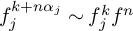in $\pi ^1(M)$ for $n \in \mathbb Z$ and $k \in K_j$ .

This gives the required dynamical series (9) over all free homotopy classes of closed orbits, their inverse, and the constant loop.

3.5 Zeta functions viewpoint

We now turn to identities on the contact analytic torsion from the viewpoint of zeta functions. On the spectral side, let

$$ \begin{align*} Z(s) = \sum_{k=0}^n (-1)^k (n+1-k) \zeta(\boldsymbol{\Delta}_Q\mid \mathcal{E}^k)(s) \,, \end{align*} $$

and on the dynamical side

$$ \begin{align*} Z^{dyn} (s) = \sum_{\gamma \in \mathcal{C}^* } \chi_\rho(\gamma) e(\gamma) |\ell(\gamma)|^{2s-1} \,, \end{align*} $$

where $e(\gamma )$ is defined by (8), and $\gamma $ ranges over all free homotopy classes of non-trivial closed orbits together with their inverse.

On the geometric side at last we consider

(42) $$ \begin{align} Z^{geo}(s) = \sum_{j \in \mathcal{S}} \chi(N_j) \chi_\rho^\zeta (f_j)(s) \,. \end{align} $$

with

$$ \begin{align*} \alpha_j^{2s} \chi_\rho^\zeta (f_j) (s) = \sum_{e^{2i \pi x}\in \operatorname{\mathrm{Spec}}^*(\rho(f_j))} & \dim V_{f_j}^x (\zeta(2s, x) + \zeta(2s,1-x)) \\ & + 2 \zeta(2s) \dim V_{f_j}^1 \end{align*} $$

where $V^x_{f_j} = \ker (\rho (f_j) - e^{2i\pi x} \operatorname {\mathrm {id}})$ , $\zeta $ is the Riemann zeta function and

(43) $$ \begin{align} \zeta(s,x) = \sum_{n \geq 0} \frac{1}{(n+x)^s} \end{align} $$

is the Hurwitz zeta function.

Theorem 3.8. On CR Seifert manifolds the functions Z and $Z^{geo}$ are meromorphic and equal, with a simple pole at $s=1/2$ .

The function $Z^{dyn}$ is meromorphic with a simple pole at $s=0$ , and one has

(44) $$ \begin{align} \Gamma(s) Z(s) = \frac{2^{-2s}}{\sqrt \pi} \Gamma(\frac{1}{2} -s) Z^{dyn} (s) \,. \end{align} $$

Moreover

$$ \begin{align*} \left\{ \begin{gathered} Z(0) = \mathrm{Res}_{0} (Z^{dyn})= - \chi^{\prime}_Q(M,\rho) \\ \mathrm{Res}_{1/2}(Z) = -\frac{1}{2\pi} Z^{dyn}(1/2)= \chi^{orb}(N) \dim V \,, \end{gathered} \right. \end{align*} $$

with

$$ \begin{align*} \chi^{\prime}_Q(M,\rho) = \sum_{k=0}^n (-1)^k (n+1-k)\dim H^k(M, \rho)\,, \end{align*} $$

using the cohomology groups of the flat bundle V over M.

This extends results obtained in [Reference Rumin and Seshadri20] in the three-dimensional case. Note also that Kitaoka computed in [Reference Kitaoka15] the spectral series $Z(s)$ on lens spaces endowed with their symmetric metric and found it reduces to a Hurwitz zeta function.

3.6 Proof of Theorem 3.8

We know from the spectral expression of $\vartheta $ that

$$ \begin{align*} \vartheta(t) = \sum_{k=0}^n (-1)^k (n+1-k) \dim \ker (\boldsymbol{\Delta}_Q \mid \mathcal{E}^k) + O (e^{-Ct}) \end{align*} $$

for some $C> 0$ when $t \rightarrow +\infty $ . According to Proposition 2.2 the limiting constant is the topological number $\chi ^{\prime }_Q(M,\rho )$ .

From $\vartheta = \vartheta ^{geo}$ , one gets using $t\rightarrow +\infty $ that

(45) $$ \begin{align} \chi^{\prime}_Q(M, \rho) = \sum_{j \in \mathcal{S}} \chi(N_j) \dim \ker (\rho(f_j) - \operatorname{\mathrm{id}})\,. \end{align} $$

Whereas when $t \rightarrow 0^+$ , the dynamical expression (9) yields

$$ \begin{align*} \vartheta(t) = \sqrt{\frac{\pi}{t}} \chi^{orb}(N) \dim V + O(e^{-C/t}) \,. \end{align*} $$

Let us consider the function

$$ \begin{align*} \vartheta_0 (t) = \vartheta(t) - c_0 \mathbf{1}_{[1,+\infty[}(t) - \frac{c_{-1/2}}{\sqrt t} \mathbf{1}_{]0,1]}(t) \end{align*} $$

with

$$ \begin{align*} c_0 = \chi^{\prime}_Q(M,\rho) \quad \mathrm{and} \quad c_{-1/2} = \sqrt \pi \chi^{orb}(N) \dim V \,. \end{align*} $$

From the previous discussion, the integral

$$ \begin{align*} I(s) = \int_0^{+\infty} \vartheta_0(t) t^{s-1} dt \end{align*} $$

coming from the Mellin transform defines a holomorphic function over $\mathbb C$ . Writing

$$ \begin{align*} \vartheta_0(t) = \vartheta(t) - c_0 + (c_0 - \frac{c_{-1/2}}{\sqrt t}) \mathbf{1}_{]0,1]}(t) \end{align*} $$

one finds first for $\Re (s)> 1/2$ that

$$ \begin{align*} I(s) = \Gamma(s) Z(s) + \frac{c_0}{s}- \frac{c_{-1/2}}{s-1/2} = \Gamma(s) Z^{geo}(s) + \frac{c_0}{s}- \frac{c_{-1/2}}{s-1/2} \,. \end{align*} $$

Using

$$ \begin{align*} \vartheta_0(t) = \vartheta^{dyn}(t) - \frac{c_{-1/2}}{\sqrt t} + (\frac{c_{-1/2}}{\sqrt t} - c_0) \mathbf{1}_{]1,+\infty]}(t) \end{align*} $$

yields for $\Re (s) < 0$ that

$$ \begin{align*} I(s) = \frac{2^{-2s}}{\sqrt \pi} \Gamma(\frac{1}{2} -s) Z^{dyn}(s) + \frac{c_0}{s} - \frac{c_{-1/2}}{s-1/2} \,. \end{align*} $$

This proves Theorem 3.8.

3.7 The contact analytic torsion from the Lefschetz and dynamical viewpoints

Recall that from (3) the contact analytic torsion is defined by $T_Q(M,\rho ) = \exp (-Z'(0)/2)$ . We shall now compute it using the previous formulae. This extends results obtained in [Reference Rumin and Seshadri20] in the three-dimensional case.

Corollary 3.9. Let M be a CR Seifert manifold endowed with a unitary representation $\rho : \pi _1 (M) \rightarrow U (d)$ . Let $N= \sqcup _{j \in \mathcal {S}} N_j$ be the decomposition of $N= M/\mathbf {S}^1$ into connected strata. Given a primitive orbit $f_j$ in $N_j$ , define

$$ \begin{align*} V^1_{f_j} = \ker (\rho(f_j) - \operatorname{\mathrm{id}}) \end{align*} $$

and denote by $\rho (f_j)^\bot $ the restriction of the holonomies to $(V^1_{f_j})^\bot $ .

Then it holds that

$$ \begin{align*} T_Q(M,\rho) = (2\pi)^{\chi^{\prime}_Q(M,\rho)} \prod_{j \in \mathcal{S}}\Bigl(\big| \det (\rho(f_j)^\bot - \operatorname{\mathrm{id}})\big|\, \alpha_j^{-\dim(V^1_{f_j}) }\Bigr)^{\chi(N_j)}\,. \end{align*} $$

Moreover one has

$$ \begin{align*} -2 \ln (T_Q(M, \rho)) = Z'(0) = \lim_{s \rightarrow 0} \big(Z^{dyn}(s) + \frac{\chi^{\prime}_Q(M,\rho)}{s} \big)\,. \end{align*} $$

The first expression coincides with that found, via topological methods, for the Reidemeister–Franz torsion by Fried [Reference Fried13, p. 198], in the case of an acyclic representation, i.e. $H^*(M,\rho ) = 0$ . Therefore, the contact analytic torsion also coincides with the (Riemannian) Ray–Singer analytic torsion in that case, from works of Cheeger and Müller [Reference Cheeger10, Reference Müller16]. The only new factor for general representations is the cohomological term $(2 \pi )^{\chi ^{\prime }_Q(M,\rho )}$ . Note that by (45) one can also write

$$ \begin{align*} T_Q(M,\rho) = \prod_{j \in \mathcal{S}}\Bigl(\big| \det (\rho(f_j)^\bot - \operatorname{\mathrm{id}})\big|\, \ell(f_j)^{\dim(V^1_{f_j}) }\Bigr)^{\chi(N_j)}\,. \end{align*} $$

The dynamical expression for the analytic torsion also extends a result proved by Fried in the acyclic case on Seifert manifolds [Reference Fried12, Thm 5.1], [Reference Fried13]. There we have

$$ \begin{align*} Z'(0)= Z^{dyn}(0) = \sum_{\gamma \in \mathcal{C}^*} \chi_\rho(\gamma) e(\gamma) /|\ell(\gamma)| \,, \end{align*} $$

which is known as the total twisted Fuller measure of periodic orbits. It has a formal invariance by deformation of the flow, as long as the orbit periods stay bounded; see [Reference Fried12, Section 4].

Proof of Corollary 3.9.

Since $Z =Z^{geo}$ is an explicit function by Theorem 3.8, we compute $(Z^{geo})'(0)$ . We follow the proof in [Reference Rumin and Seshadri20, p. 771] which we recall for completeness.

From [Reference Whittaker and Watson23, p. 271], one has for $x \in ]0,1[$ , $\zeta (0, x) = \frac {1}{2} -x $ , hence $\zeta (0,x) + \zeta (0,1-x) = 0$ . Also by Lerch’s formula $\partial _s \zeta (s,x)_{s=0} = \ln \Gamma (x) - \frac {1}{2} \ln (2\pi )$ , it holds that $\zeta '(0) = - \frac {1}{2} \ln (2\pi )$ and

$$ \begin{align*} \partial_s \zeta(s,x)_{s=0} + \partial_s \zeta(s,1-x)_{s=0} &= \ln (\Gamma(x)\Gamma(1-x) /2\pi) = - \ln (2 \sin(\pi x)) \\ & = -\ln |1 - e^{2i\pi x}| \,. \end{align*} $$

Hence from (42), one finds that

$$ \begin{align*} \chi_\rho^\zeta (f_j)'(0) + 2 \ln(\alpha_j) \chi_\rho^\zeta (f_j)(0) & = - 2 \ln |\det ( \rho(f_j)^\bot - \operatorname{\mathrm{id}})| -2 \dim V^1_{f_j} \ln (2 \pi) \,. \end{align*} $$

Summing these results using the formula (42) for $Z^{geo}$ and (45) gives the first result for $T_Q(M,\rho )$ .

For the second one, it is useful to observe that

(46) $$ \begin{align} 2 \Gamma(2s) \cos (\pi s) Z = Z^{dyn} \,, \end{align} $$

as follows by multiplying (44) by $\Gamma (s+1/2)$ and using the classical identities

$$ \begin{align*} \Gamma(s) \Gamma(s + \frac{1}{2}) = 2^{1-2s} \sqrt \pi \Gamma(2s)\quad \mathrm{and} \quad \Gamma(s+ \frac{1}{2}) \Gamma(s - \frac{1}{2}) = \frac{\pi}{ \cos \pi s}\,. \end{align*} $$

One knows from Theorem 3.8 that $Z(0) = - \chi ^{\prime }_Q(M,\rho )$ . Hence developing (46) when $s\rightarrow 0$ gives the dynamical formula for $T_Q(M,\rho )$ .

4.1 The contact eta trace from the topological viewpoint

We start the study of the eta trace spectral series involved in the eta invariant of $S_Q$ . From (11) it reads

$$ \begin{align*} \vartheta_S (t) = \operatorname{\mathrm{Tr}} (\sqrt t S_Q e^{-t\boldsymbol{\Delta}_Q})\,. \end{align*} $$

We complete arguments already sketched in Section 1.5. From Proposition 4.1, one has $\sigma P S_Q = -S_Q \sigma P$ with $\sigma P = -P \sigma $ . Therefore the spectrum of $S_Q = P + \sigma T$ is symmetric with respect to zero, except on $\mathcal {H}_S = \ker P$ and the eta trace $\vartheta _S$ retracts on it with $S_Q = \sigma T$ . Hence

$$ \begin{align*} \boldsymbol{\Delta}_Q = S_Q^2= -T^2 \quad \mathrm{on} \quad \mathcal{H}_S \,. \end{align*} $$

One can split the domain $\mathcal {E}_S$ of $S_Q$ and $\mathcal {H}_S$ with respect to the action of the involution $\tau = i\sigma = \pm 1 $ . We have

$$ \begin{align*} \vartheta_S(t) = -\sqrt t(\operatorname{\mathrm{Tr}} (iT e^{tT^2} \mid \mathcal{H}_S^+) - \operatorname{\mathrm{Tr}}(iT e^{tT^2 } \mid \mathcal{H}_S^-))\,. \end{align*} $$

On CR Seifert manifolds, the V-valued forms in $\mathcal {H}_S$ split under Fourier decomposition as in Sections 3.1–3.2. Hence we obtain the identity:

Theorem 4.4. One has on connected CR Seifert manifolds

$$ \begin{align*} \vartheta_S(t) = \vartheta_S^{top}(t) =- \sqrt t \sum_{\lambda \operatorname{\mathrm{Spec}}(iT)} \operatorname{\mathrm{ind}}( P^+ \mid V_\lambda) \lambda e^{-t\lambda^2} \,, \end{align*} $$

where $P^+ = P : \mathcal {E}_S^+ \rightarrow \mathcal {E}_S^-$ .

We shall now describe the index involved.

4.2 From the topological to the geometric expression for $\vartheta _S$ .

Let $*_H$ denote the $*$ operator on the Hermitian space H. From [Reference Weil22, Thm. 2] one has

$$ \begin{align*} *_H L^r \alpha = L^r((-1)^{p(p+1)/2} J \alpha) = L^r(\sigma \alpha) \end{align*} $$

on $\Omega ^p_0 H = \mathcal {E}^p$ when $p+2r = n$ . That means that the involution $\tau = i\sigma $ on $\mathcal {E}_S$ is conjugated to $\tau _H = i*_H$ on $\Omega ^nH$ through the Lefschetz decomposition

$$ \begin{align*} \mathcal{E}_S \simeq \Omega^n H\quad \mathrm{with} \quad \mathcal{E}_S^{\tau = \pm 1} \simeq (\Omega^nH)^{\tau_H = \pm 1} \,. \end{align*} $$

From these isomorphisms, $P^+ : \Omega ^{n,+} H \rightarrow \Omega ^{n,-}H$ . Hence its elliptic symbol class as seen from N is associated to the signature index on N; see [Reference Atiyah, Patodi and Singer5, Section 6]. Then let $\mathcal {L}(N)_{orb}$ denote the Hirzebruch L-genus of the orbifold N. As in Section 3.2 we have by the Kawasaki index theorem and [Reference Atiyah, Patodi and Singer5]

$$ \begin{align*} \operatorname{\mathrm{ind}}(P^+ \mid V_\lambda) = \langle \operatorname{\mathrm{ch}}(V_\lambda) \wedge \mathcal{L}(N)_{orb}, [N] \rangle_{orb} \,, \end{align*} $$

and $\vartheta _S(t)$ can be written

(50) $$ \begin{align} \vartheta_S(t) = - \langle \operatorname{\mathrm{ch}}(V)^{\theta}_{odd}(t)\wedge \mathcal{L}(N)_{orb}, [N] \rangle_{orb} \,. \end{align} $$

using the notation

(51) $$ \begin{align} \operatorname{\mathrm{ch}}(V)^{\theta}_{odd}(t) = \sum_{\lambda \in \operatorname{\mathrm{Spec}}(iT)} \sqrt t \lambda \operatorname{\mathrm{ch}}(V_\lambda)e^{-t \lambda^2} \,. \end{align} $$

We need to study this ‘ $\theta $ -regularised’ Chern character of V, which is seen as an infinite dimensional bundle from N by (4). It is also useful to consider its even version

(52) $$ \begin{align} \operatorname{\mathrm{ch}}(V)^{\theta}_{ev}(t) = \sum_{\lambda \in \operatorname{\mathrm{Spec}}(iT)} \operatorname{\mathrm{ch}}(V_\lambda)e^{-t \lambda^2} \,. \end{align} $$

Note that its zero degree part already showed up in (34) in the study of the topological series for the torsion function, that satisfies

$$ \begin{align*} \vartheta^{top} (t) = \langle \operatorname{\mathrm{ch}}(V)^\theta_{ev}(t) \wedge e(N)_{orb} , [N] \rangle_{orb} \,. \end{align*} $$

From (50) we now need to compute these differential forms in their entirety.

The expressions for the G-equivariant Chern class and Hirzebruch L-genus being quite involved in general, see [Reference Atiyah and Singer6, Thm. 6.12], we will restrict ourselves to the case where the singular set of N is finite, i.e. the exceptional orbits $f_i$ are isolated.

This is always satisfied in dimension three because the singular set is at of at least codimension two. In higher dimension, following Section 3.2, that means that all the eigenvalues of the ‘isotopy’ matrices $M_j$ of the strata are of order $\alpha _j$ exactly. In that case one has $\ker (M_j^k - \operatorname {\mathrm {id}}) = \ker (M_j - \operatorname {\mathrm {id}})$ unless $k \in \mathbb Z \alpha _j$ and the summation sets $K_j$ used in Kawasaki’s formula, see (36), reduce to $(\mathbb Z\alpha _j)^c$ . Using Atiyah–Bott’s work [Reference Atiyah and Bott3, Section 6], one can identify the contribution of the isolated singular orbits, and the orbifold pairing in (50) decomposes as follows

(53) $$ \begin{align} \langle \operatorname{\mathrm{ch}}(V)^{\theta}_{odd}(t)\wedge \mathcal{L}(N)_{orb}, [N] \rangle_{orb} = \langle & \operatorname{\mathrm{ch}}(V)^\theta_{odd}(t) \wedge \mathcal{L}(N) , [N_{smooth}] \rangle \\ & + \sum_j \frac{1}{\alpha_j} \sum_{r=1}^{\alpha_j-1} \operatorname{\mathrm{ch}}(V)^\theta_{odd}(f_j^r)(t) \nu(f_j^r) \,,\nonumber \end{align} $$

where, for $\gamma = f_j^n$ with $n\not \equiv 0 \mod \alpha _j$ ,

$$ \begin{align*} \nu(\gamma)= i (-1)^k \prod_{m=1}^{2k-1} \cot (\theta_m(\gamma)/2) \end{align*} $$

for angles $\theta _m(\gamma )$ associated to the unitary return map $d \tau _\gamma $ along $\gamma $ in $H_{p_j}$ and $\dim N = 4k-2$ . Note that these angles are non-zero since the singular orbits $f_j$ are isolated.

It remains to express the regularised Chern characters of V. To compute first the Chern character of $V_\lambda $ , as seen from N, we use the following twisted connection

$$ \begin{align*} \nabla^\lambda = \nabla^\rho + i \lambda \theta \,, \end{align*} $$

where $\nabla ^\rho $ is the flat connection on V. Since $\nabla ^\lambda _T s = 0$ on sections of $\mathbf {V}_\lambda $ , this connection descends to M as a connection on $V_\lambda $ . Its curvature form is given for $X,Y \in H$ by

$$ \begin{align*} R_{\nabla^\lambda}(X,Y) & = \nabla^\lambda_X \nabla^\lambda_Y - \nabla^\lambda_Y \nabla^\lambda_X - \nabla^\lambda_{[X,Y]} \\ & = R_{\nabla^\rho} (X,Y) + i \lambda d\theta(X,Y) \\ & = i \lambda d\theta(X,Y)\,. \end{align*} $$

Hence the bundle $(V_\lambda , \nabla _\lambda )$ has curvature form $\Omega _\lambda = i \lambda d\theta \otimes \operatorname {\mathrm {id}}_{V_\lambda }$ . Then let

$$ \begin{align*} \mathbf{c} = -\frac{d \theta}{2\pi} \,. \end{align*} $$

Note that $\mathbf c = c_1(L)$ is the first Chern class of the line bundle L over N whose circle bundle is M. Using the V-bundle structure of $V_\lambda $ as given in (33), one obtains that

$$ \begin{align*} \operatorname{\mathrm{ch}} (V_\lambda) = \operatorname{\mathrm{Tr}}(e^{\frac{i \Omega_\lambda}{2\pi}}) = \dim V^x e^{\lambda \mathbf c}\,. \end{align*} $$

over smooth points of N, while the equivariant Chern character at $f_j^r$ is

$$ \begin{align*} \operatorname{\mathrm{ch}}(V_\lambda)(f_j^r) = e^{- 2i \pi r\lambda/\alpha_j } \chi_\rho(f_j^r \mid V^x)\,. \end{align*} $$

This leads to the geometrical and dynamical expressions for the $\theta $ -regularised Chern characters $\operatorname {\mathrm {ch}}(V)^\theta _{ev}$ and $\operatorname {\mathrm {ch}}(V)^\theta _{odd}$ using the classical Jacobi theta function $\theta (x,t) = \sum _{n \in \mathbb Z} e^{-t(n+x)^2}$ and the Poisson formula (39) as in Section 3.4.

Proposition 4.5. $\bullet $ Over smooth orbits, it holds that

$$ \begin{align*} \operatorname{\mathrm{ch}}(V)^\theta_{ev} (t) & = \sum_{\lambda \in \operatorname{\mathrm{Spec}}(iT)} \dim V^x e^{\lambda \mathbf c - t \lambda^2} \\ & = \sum_{e^{2i\pi x} \in \operatorname{\mathrm{Spec}} (\rho(f))}\dim V^x e^{\mathbf c^2/4t}\theta (x - \frac{\mathbf c}{2t},t) \\ & = \frac{\ell(f)}{\sqrt{4\pi t}} \sum_{n \in \mathbb Z} \chi_\rho(f^n) e^{- (\ell(f^n) + i \mathbf c)^2/ 4t} \end{align*} $$

and

$$ \begin{align*} \operatorname{\mathrm{ch}}(V)^\theta_{odd}(t) & = \sqrt t \sum_{\lambda \in \operatorname{\mathrm{Spec}}(iT)} \dim V^x \lambda e^{\lambda \mathbf c -t \lambda^2} \\ & = \sqrt t \frac{d}{d\mathbf c} \operatorname{\mathrm{ch}}(V)^\theta_{ev} (t)\\ & = - \frac{i \ell(f)}{4t\sqrt{\pi}} \sum_{n \in \mathbb Z} \chi_\rho(f^n)(\ell(f^n) + i \mathbf c) e^{- (\ell(f^n) + i \mathbf c)^2/ 4t} , \end{align*} $$

in terms of formal derivation as a polynomial in $\mathbf c$ .

$\bullet $ At a singular orbit $f_j^r$ , the equivariant $\theta $ -Chern character satisfies

$$ \begin{align*} \operatorname{\mathrm{ch}}(V)^\theta_{ev}(f_j^r)(t) & = \sum_{\lambda \in \operatorname{\mathrm{Spec}}(iT)} \chi_\rho(f_j^r \mid V^x) e^{-2i\pi r \lambda/\alpha_j -t \lambda^2}\\ & = \sum_{e^{2i\pi x}\in \operatorname{\mathrm{Spec}}(\rho(f))} \chi_\rho(f_j^r \mid V^x) e^{-\pi^2 r^2/t\alpha_j^2} \theta(x + i \frac{\pi r}{t \alpha_j},t) \\ & = \frac{\alpha_j \ell(f_j)}{\sqrt{4 \pi t}}\sum_{n \in \mathbb Z} \chi_\rho(f_j^{r + n \alpha_j}) e^{-\ell(f_j^{r+ n\alpha_j})^2/4t} \end{align*} $$

and

$$ \begin{align*} \operatorname{\mathrm{ch}}(V)^\theta_{odd}(f_j^r)(t) & = \sqrt t \sum_{\lambda \in \operatorname{\mathrm{Spec}}(iT)} \chi_\rho(f_j^r \mid V^x) \lambda e^{-2i\pi r \lambda/\alpha_j -t \lambda^2}\\ & = - \frac{i \alpha_j \ell(f_j)}{4t \sqrt{\pi}}\sum_{n \in \mathbb Z} \chi_\rho(f_j^{r+ n \alpha_j})\ell(f_j^{r + n \alpha_j}) e^{- \ell(f_j^{r + n\alpha_j})^2/ 4t} \,. \end{align*} $$

Note the similar expressions for regular and discrete orbits. All the homotopy classes of closed orbits of the circle action, together with their opposite, enter only once in the various contributions. We also observe that the spectral–dynamical duality in our Selberg–type trace formulae actually shows up at the level of these $\theta $ -regularised Chern characters, and only depends on the classical Poisson formula for the heat kernel on the circle.

Using Proposition 4.5 in (53), we obtain a dynamical expression for the contact eta function.

Theorem 4.6. On a connected CR Seifert manifold with finite singular orbits, one has

$$ \begin{align*} \vartheta_S(t) = \vartheta_S^{dyn}(t)= \frac{1}{\sqrt {4 \pi}} \sum_{\gamma \in \mathcal{C}} \chi_\rho(\gamma) \sigma(\gamma)(t) \,. \end{align*} $$

where powers of the generic orbit $\gamma = f^n$ , with $n \in \mathbb Z$ , contribute to

$$ \begin{align*} \sigma(\gamma)(t) = \frac{i \ell(f)}{2t} \, \big\langle (\ell(\gamma) + i \mathbf c) e^{-(\ell (\gamma) + i \mathbf c)^2 /4t} \wedge \mathcal{L}(N), [N_{smooth}] \big\rangle \,, \end{align*} $$

while powers of the singular orbits $\gamma = f_j^p$ , with $p \not \equiv 0 \mod \alpha _j$ , contribute to

$$ \begin{align*} \sigma(\gamma)(t) = \frac{i \ell(f_j)}{2t} \ell(\gamma) e^{-\ell(\gamma)^2/4t} \, \nu(\gamma) \,. \end{align*} $$

4.3 Applications to the contact eta function $\eta (S_Q)(s)$

In order to get applications to the contact eta invariant we now need to study our theta–regularised contact eta function $\vartheta _S$ from its ‘zeta’ viewpoint $\eta (S_Q)(s)$ .

We first study the odd zeta regularised Chern character of V, i.e. the series

$$ \begin{align*} \operatorname{\mathrm{ch}}(V)^{\zeta}_{odd}(s) = \sum_{\lambda \in \operatorname{\mathrm{Spec}}^*(iT)} \frac{\lambda \operatorname{\mathrm{ch}}(V_\lambda)}{|\lambda|^{2s+1}} = \sum_{\lambda \in \operatorname{\mathrm{Spec}}^*(iT)} \dim V^x \frac{\lambda e^{\lambda \mathbf c}}{|\lambda|^{2s+1}} \,. \end{align*} $$

We proceed by taking the Mellin transform of $\operatorname {\mathrm {ch}}(V)^{\theta }_{odd}(t)$ . From Proposition 4.5 its smooth part reads

$$ \begin{align*} \operatorname{\mathrm{ch}}(V)^{\theta}_{odd}(t) & = \sqrt t \sum_{\lambda \in \operatorname{\mathrm{Spec}}(iT)} \dim V^x \lambda e^{\lambda \mathbf c -t \lambda^2} \\ & = \sum_{\lambda \in \operatorname{\mathrm{Spec}}^*(iT)} \dim V^x \sum_{p=0}^{2k-1} \frac{\mathbf c^p}{p!} \lambda^{p+1} \sqrt t e^{-t \lambda^2} \,, \end{align*} $$

with $\dim N = 4k -2$ . Then one finds by dominated convergence and direct computation that for $\Re (s)> k$ the following integral converges and

$$ \begin{align*} I(s) = \int_0^{+\infty} \operatorname{\mathrm{ch}}(V)^{\theta}_{odd}(t) t^{s-1} dt = \Gamma(s+\frac{1}{2}) \sum_{p=0}^{2k-1} \frac{\mathbf c^p}{p!} \sum_{e^{2i \pi x} \in \operatorname{\mathrm{Spec}}(\rho(f))} Z(p,s,x) \end{align*} $$

with

(54) $$ \begin{align} Z(p,s,x) = \begin{cases} \dim V^x (\zeta(2s-p, x) +(-1)^{p+1} \zeta(2s-p, 1-x)) & \quad \mathrm{if} \ 0< x <1 \\ \dim V^1 (1+(-1)^{p+1})\zeta(2s-p) & \quad \mathrm{if}\ x=1 \end{cases} \end{align} $$

where $\zeta (s,x)$ is the Hurwitz zeta function (43). Therefore $I(s)/\Gamma (s + \frac {1}{2})$ defines a meromorphic function with possible simple poles at $s = \frac {j}{2}$ for $j \in [[ 1, 2k]]$ . Hence we get that the series

(55) $$ \begin{align} \operatorname{\mathrm{ch}}(V)^{\zeta}_{odd}(s) & = \sum_{\lambda \in \operatorname{\mathrm{Spec}}(iT)*} \lambda \frac{\operatorname{\mathrm{ch}}(V_\lambda)}{|\lambda|^{2s+1}} = \frac{I(s)}{\Gamma(s+\frac{1}{2})} \\ & = \sum_{p=0}^{2k-1} \frac{\mathbf c^p}{p!} \sum_{e^{2i \pi x} \in \operatorname{\mathrm{Spec}}(\rho(f))} Z(p,s,x) \nonumber \end{align} $$

are well defined and meromorphic on the same domain.

On the discrete part $\operatorname {\mathrm {ch}}(V)^\theta _{odd}(f_j^r)$ as given in Proposition 4.5, one finds that for $\Re (s)> 1/2$

(56) $$ \begin{align} \operatorname{\mathrm{ch}}(V)^\zeta_{odd}(f_j^r)(s) = \sum_{e^{2i\pi x} \in \operatorname{\mathrm{Spec}}(\rho(f))} \chi_\rho(f_j^r\mid V^x) Z(f_j^r,s,x) \end{align} $$

with

(57) $$ \begin{align} & Z(f_j^r,s,x) = \\ \nonumber & \begin{cases} e^{-2i \pi rx /\alpha_j} L (e^{-2 i \pi r / \alpha_j}, 2s,x) - e^{2i \pi r (1-x)/\alpha_j} L (e^{2 i \pi r / \alpha_j}, 2s,1-x) & \ \mathrm{for}\ 0< x < 1 \\ e^{-2i \pi r/\alpha_j} L(e^{-2i \pi r/ \alpha_j},2s,1) - e^{2i\pi r / \alpha_j}L(e^{2i\pi r /\alpha_j},2s,1) & \ \mathrm{for}\ x =1 \,. \end{cases} \end{align} $$

where

$$ \begin{align*} L(z,s,x) = \sum_{n \geq 0}\frac{z^n}{(n+ x)^s} \end{align*} $$

is the Lerch zeta function. In our case, $z=e^{\pm 2i \pi r /\alpha _j}$ is a root of unity and

(58) $$ \begin{align} L(z,s,x) = \frac{1}{\alpha_j^{s}} \sum_{m=0}^{\alpha_j-1} z^m \zeta(s, \frac{m+x}{\alpha_j}) \end{align} $$

splits into a sum of Hurwitz zeta functions. From [Reference Apostol2, p. 255], $\zeta (s,x)$ is analytic with a simple pole at $s=1$ and residue $1$ . Therefore $\mathrm {Res}_{s=1/2} L(e^{\pm 2i\pi r /\alpha _j}, 2s,0)=0$ and the functions $Z(f_j^r,s,x)$ are entire.

This gives an explicit geometric expression for $\operatorname {\mathrm {ch}}(V)^\zeta _{odd}(s)$ that leads with (50) and (53) to the formula for $\eta (S_Q)(s)$ from

(59) $$ \begin{align} - \eta(S_Q)(s) & = \langle \operatorname{\mathrm{ch}}(V)^\zeta_{odd}(s) \wedge \mathcal{L}(N)_{orb}, [N] \rangle_{orb} \\ & = \langle \operatorname{\mathrm{ch}}(V)^\zeta_{odd}(s) \wedge \mathcal{L}(N) , [N_{smooth}] \rangle + \sum_i \frac{1}{\alpha_i} \sum_{r=1}^{\alpha_i-1} \operatorname{\mathrm{ch}}(V)^\zeta_{odd}(f_i^r)(s) \nu(f_i^r) \,.\nonumber \end{align} $$

Specialising at the regular value $s=0$ gives an explicit formula for the contact eta invariant $\eta (S_Q)(0)$ . Let

$$ \begin{align*} B(t,x) = \frac{t e^{tx}}{e^t-1} = \sum_{n=0}^{+\infty} B_n(x) \frac{t^n}{n!} \end{align*} $$

be the generating function of Bernoulli polynomials; see e.g. [Reference Apostol2], and

$$ \begin{align*} B_{ev}(t,x) = t\frac{\cosh(t(x-\frac{1}{2}))}{2 \sinh(\frac{t}{2})} = \sum_{n=0}^{+\infty} B_{2n}(x) \frac{t^{2n}}{(2n)!} \end{align*} $$

its even part in t. We consider the function

$$ \begin{align*} (\Delta B_{ev})(t,x) & = \frac{1}{t}(B_{ev}(t,x) -1) = \sum_{n=1}^{+\infty} B_{2n}(x) \frac{t^{2n-1}}{(2n)!} \\ & = \frac{\cosh(t(x-\frac{1}{2}))}{2 \sinh(\frac{t}{2})} - \frac{1}{t}\,. \end{align*} $$

We shall also need

$$ \begin{align*} \widetilde B (t,x) = \begin{cases} B(t,x) & \mathrm{for} \ 0< x <1 \\ \frac{1}{2}(B(t,1) + B(t,0)) & \mathrm{for}\ x= 1 \,. \end{cases} \end{align*} $$

In the following statement, we recall that $V_f^x = \ker (\rho (f) - e^{2i \pi x} \operatorname {\mathrm {id}})$ for $0< x \leq 1$ .

Theorem 4.8. On a connected CR Seifert manifold with finite singular orbits, it holds that

$$ \begin{align*} \eta(S_Q)(0) = 2 & \sum_{e^{2i\pi x}\in \operatorname{\mathrm{Spec}}(\rho(f))} \dim V_f^x \langle (\Delta B_{ev})(\mathbf c, x) \wedge \mathcal{L}(N), [N]_{smooth} \rangle \\ &\qquad\qquad\qquad + 2 \sum_{e^{2i\pi x}\in \operatorname{\mathrm{Spec}}(\rho(f))} \sum_j \frac{1}{\alpha_j} \sum_{r=1}^{\alpha_j-1} \chi_\rho(f_j^r \mid V_f^x) \frac{\widetilde B(-2 i \pi r/ \alpha_j, x)}{-2i \pi r /\alpha_j} \nu(f_j^r) \,. \end{align*} $$

Proof. We have to evaluate $Z(0,p,x)$ as given in (54). From e.g. [Reference Apostol2, p. 264], we know that

$$ \begin{align*} \zeta(-p,x) = - \frac{B_{p+1}(x)}{p+1} \quad \mathrm{for}\ p \in\mathbb N \,. \end{align*} $$

Moreover $B_n(1-x) = (-1)^n B_n(x)$ , so that $Z(0,x,p) = 0$ for p even, while for p odd

$$ \begin{align*} Z(0,x,p) = - 2 \dim V^x \frac{B_{p+1}(x)}{p+1} \,. \end{align*} $$

Hence from (55)

$$ \begin{align*} \operatorname{\mathrm{ch}}(V)^\zeta_{odd}(0) & = -2 \sum_{e^{2i \pi x} \in \operatorname{\mathrm{Spec}}(f)} \dim V_f^x \sum_{p=1\, p\,odd}^{2k-1} B_{p+1}(x) \frac{\mathbf c^p}{(p+1) !}\\ & = -2 \sum_{e^{2i \pi x} \in \operatorname{\mathrm{Spec}}(f)} \dim V_f^x (\Delta B_{ev})(\mathbf c, x) \,, \end{align*} $$

as needed. Note that one can replace $\Delta B_{ev}$ by $\Delta B$ in the formula for $\eta (S_Q)(0)$ since $\langle (\Delta B_{odd}(\mathbf c, x) \wedge \mathcal {L}(N), [N]_{smooth}\rangle = 0$ for dimensional reasons.

We compute the discrete contribution of $f_j^r$ . Let $z= e^{\pm 2 i \pi r/\alpha _j}$ . From $\zeta (0, x) = 1/2 -x$ and (58), one gets

$$ \begin{align*} L(z,0, x) & = \sum_{m=0}^{\alpha_j -1} z^m(\frac{1}{2} - \frac{m+x}{\alpha_j}) =- \frac{1}{\alpha_j} \sum_{m=0}^{\alpha_j-1} m z^m \\ & = \frac{1}{1 -z} \,, \end{align*} $$

by differentiating the identity $\displaystyle \sum _{m=0}^{\alpha _i -1} u^{m+1} = \frac {u(1-u^{\alpha _j})}{1 -u}$ at $u=z$ . Inserting it in (57) gives the result.

4.4 Comparison with related results

Theorem 4.8 generalises an expression given in [Reference Biquard, Herzlich and Rumin7, Theorem 8.8] in the three-dimensional case and with a trivial representation. (Note that in [Reference Biquard, Herzlich and Rumin7], $\zeta (P)(s)$ includes $\dim \ker P$ by convention.) There one has

$$ \begin{align*} \eta(S_Q)(0) = \eta (*D + d_Q \delta_Q)(0) = \eta_0(M, \theta) - 1 \,, \end{align*} $$

where $\eta _0(M, \theta )= \mathrm {FP}_{\varepsilon =0}\,\eta (*_{g_\varepsilon } d)$ is the renormalised eta invariant of $*_{g_\varepsilon } d$ for the sub-Riemannian limit of metrics $g_\varepsilon = d \theta (\cdot , J \cdot ) + \varepsilon ^{-1}\theta ^2$ when $\varepsilon \rightarrow 0$ . From [Reference Biquard, Herzlich and Rumin7, Section 3], this also coincides with the adiabatic limit of $\eta (*_{g_\varepsilon } d)$ for $\varepsilon \rightarrow +\infty $ in our fibred case.

In general dimension, the formula for $\eta (S_Q)(0)$ in Theorem 4.8 no longer shows global (over M) cohomological terms, in contrast then to $\eta (*D)(0)$ by Proposition 4.2. This is related to the fact that the spectrum of $S_Q$ is more symmetric than the one of $*D$ by Proposition 4.1. While $*D$ acts on a smaller space than $S_Q$ , it contains un-symmetrised copies of zeta functions of Laplacians, leading to additional cohomological terms at $s=0$ .

Also, from [Reference Albin and Quan1], one knows that $\eta (*D)(0)$ compares on general contact manifolds with the renormalised sub-Riemannian limit $\eta _0(M,\theta )= FP_{\varepsilon =0} (*{g_\varepsilon } d)$ , up to local terms. It coincides with the adiabatic limit of the eta invariant in our CR Seifert situation. This limit has been studied in depth by other means. Building on previous works by Bismut and Cheeger [Reference Bismut and Cheeger8], Dai [Reference Dai11] and Zhang [Reference Zhang24] expressed $\eta _0(M, \theta )$ for circle bundles, in the case of a trivial representation and a smooth quotient N. Taking into account that their eta invariant is twice ours, which is defined using $*D$ only instead of $*D + D*$ , one sees from [Reference Dai11, Theorem 0.3] and [Reference Zhang24, Theorem 1.7] that

(60) $$ \begin{align} \eta_0(M,\theta) = 2 \langle \Delta B_{ev}(\mathbf c, 1) \wedge \mathcal{L}(N), [N]\rangle + \tau \end{align} $$

where $\tau $ is the signature of the ‘collapsing spectrum’ in the adiabatic limit. More precisely, from [Reference Dai11, Section 4.3], $\tau $ is computed using the Leray spectral sequence of the fibration $\mathbf {S}^1 \rightarrow M \rightarrow N$ .

We briefly present this in relation to Proposition 4.2. From [Reference Dai11], (12) and Section 2.2, one finds that the $E_2$ -term of the Leray spectral sequence identifies with

$$ \begin{align*} \ker T \cap \ker d_H \cap \ker \delta_H = \ker \boldsymbol{\Delta}_Q \,, \end{align*} $$

where $\boldsymbol {\Delta }_Q$ is acting diagonally on horizontal, vertical and Lefschetz components of $\Omega ^*M$ . Then, following [Reference Dai11], $\tau $ is the signature of the symmetric bilinear form

$$ \begin{align*} Q : E_2^{2k-1,\theta} \otimes E_2^{2k-1,\theta} & \rightarrow \mathbb R\\ \alpha \otimes \beta & \mapsto \int_M \alpha \wedge d_2 \beta \,. \end{align*} $$

using the second differential of the Leray spectral sequence

$$ \begin{align*} d_2 : E_2^{2k-1,\theta} & \rightarrow E_2^{2k}\\ \theta \wedge \alpha & \mapsto L \alpha \end{align*} $$

Now, by e.g. [Reference Weil22, Theorem 2], one has for $\alpha \in \mathcal {E}^{2p}$

$$ \begin{align*} *_H \alpha = \frac{1}{(2k-1 - 2p)!} L^{2k-1 - 2 p} \sigma \alpha \,, \end{align*} $$

and therefore

$$ \begin{align*} Q(\theta \wedge L^{k-p-1}\alpha , \theta \wedge L^{k-p-1} \beta) & = \int_M \theta \wedge L^{2k-2p-1} \alpha \wedge \beta \\ & = (2k-1 - 2p)! \int_M (\sigma \alpha , \beta)\, \mathrm{dvol} \,, \end{align*} $$

from which it follows that

$$ \begin{align*} \tau = \mathrm{Signature}\, (Q) = \sum_{0 \leq a+b=2p \leq 2 (k-1)} (-1)^p i^{a-b} \dim H^{a,b}(M) \,. \end{align*} $$

This is the cohomological sum in Proposition 4.2. Hence, for smooth quotient N and trivial representation, this relates (60) to the equations

$$ \begin{align*} \eta_0(M,\theta) = \eta(S_Q)(0) + \tau = \eta (*D)(0) + \mathrm{local \ terms}\,. \end{align*} $$

We note in conclusion that in the adiabatic viewpoint, the term $2 \langle \Delta B_{ev}(\mathbf c, 1) \wedge \mathcal {L}(N), [N]\rangle $ comes from the analysis of an eta form constructed by Bismut and Cheeger [Reference Bismut and Cheeger8]. It is associated to a Dirac operator for a superconnection over the fibres. Here, in this smooth case, from our viewpoint

$$ \begin{align*} 2 \langle \Delta B_{ev}(\mathbf c, 1) \wedge \mathcal{L}(N), [N]\rangle = \eta(S_Q)(0) \,, \end{align*} $$

so that this term is interpreted as being the eta invariant of a second order hypoelliptic differential operator over the whole contact manifold M.

4.5 The contact eta function from the dynamical viewpoint

We eventually work out the dynamical aspect of the eta function and eta invariant. We start with the smooth part. From Proposition 4.5 we have that for some $a>0$

$$ \begin{align*} \operatorname{\mathrm{ch}}(V)^\theta_{odd}(t) = O(e^{-at}) \quad \mathrm{when} \quad t \rightarrow +\infty \,. \end{align*} $$

We study the behaviour of $\operatorname {\mathrm {ch}}(V)^\theta _{odd}(t)$ when $t \rightarrow 0^+$ . Its dynamical expression contains terms $e^{-(\ell (\gamma ) + i \mathbf c)^2/4t}$ with $\gamma = f^n$ that can be written

$$ \begin{align*} e^{-(\ell(\gamma) + i \mathbf c)^2/4t} &= e^{- \ell^2(\gamma)/4t} e^{ (- 2 i\mathbf c \ell(\gamma) +\mathbf c^2)/4t} \\ &= e^{- \ell^2(\gamma)/4t} \sum_{p=0}^{2k-1} \frac{1}{p !} \Bigl(\frac{-2i \mathbf c\ell(\gamma) + \mathbf c^2 }{4t} \Bigr)^p\\ & = O(e^{-\ell^2(\gamma)/8t}) \end{align*} $$

when $t \rightarrow 0^+$ and $n \not =0$ . Therefore the divergence of $\operatorname {\mathrm {ch}}(V)^\theta _{odd}(t)$ when $t\rightarrow 0$ only comes from the trivial constant orbit and one has for some $b>0$

$$ \begin{align*} \operatorname{\mathrm{ch}}(V)^\theta_{odd} (t) - \dim V \frac{\ell (f) \mathbf c}{4t \sqrt{\pi}} e^{\mathbf c^2/4t} = O(e^{-b/t}) \,, \end{align*} $$

with

$$ \begin{align*} \frac{\mathbf c}{4t} e^{\mathbf c^2/4t} = \sum_{p=0}^{k-1} \frac{\mathbf c^{2p+1}}{p! (4t)^{p+1}} \,. \end{align*} $$

This shows that the function

$$ \begin{align*} f(t) = \operatorname{\mathrm{ch}}(V)^\theta_{odd}(t) - \dim V \frac{\ell(f)\mathbf c}{4t \sqrt \pi} e^{\mathbf c^2/4t} \mathbf{1}_{]0,1]}(t) \end{align*} $$

has an entire Mellin transform over $\mathbb C$ . Proceeding as in Section 3.6 we first find that for $\Re (s)> k$

$$ \begin{align*} I(s) = \int_0^{+\infty} f(t) t^{s-1} dt & = \Gamma(s + \frac{1}{2}) \operatorname{\mathrm{ch}}(V)^\zeta_{odd}(s) \\ &\quad - \dim V \sum_{p=0}^{k-1}\frac{\ell(f) \mathbf c^{2p+1}}{p! 4^{p+1} \sqrt \pi} \times \frac{1}{s-p-1} \,, \end{align*} $$

While writing

$$ \begin{align*} f(t) = \operatorname{\mathrm{ch}}(V)^\theta_{odd}(t) - \dim V \frac{\ell(f) \mathbf c}{4t \sqrt \pi} e^{\mathbf c^2/4t} + \dim V \frac{ \ell(f) \mathbf c }{4t \sqrt \pi} e^{\mathbf c^2/4t} \mathbf{1}_{]1,+\infty]}(t) \end{align*} $$

and using the dynamical expression for $\operatorname {\mathrm {ch}}(V)^\theta _{odd}(t)$ one has for $\Re (s) < 0$

$$ \begin{align*} I(s) = \Gamma(1 - s)\big( & \sum_{n \in \mathbb Z^*}- \frac{i\ell(f)}{4^s\sqrt \pi} \chi_\rho(f^n) (\ell(f^n) + i\mathbf c) \big( (\ell(f^n) + i\mathbf c)^2\big)^{s-1} \big)\\ & - \dim V\sum_{p=0}^{k-1}\frac{ \ell(f) \mathbf c^{2p+1}}{p! 4^{p+1} \sqrt \pi} \times \frac{1}{s-p-1} \,. \end{align*} $$

Here $z^s$ denotes the principal branch of the power function. We then get the identity of meromorphic functions through analytic continuation

$$ \begin{align*} \Gamma(s+1/2) \operatorname{\mathrm{ch}}(V)^\zeta_{odd}(s) = \Gamma(1-s) \sum_{n \in \mathbb Z^*}- \frac{i\ell(f)}{4^s\sqrt \pi} \chi_\rho(f^n) (\ell(f^n) + i\mathbf c) \big( (\ell(f^n) + i\mathbf c)^2\big)^{s-1} \,. \end{align*} $$

One more easily finds the discrete dynamical contribution of $f_j^r$ due to rapid decay of $\operatorname {\mathrm {ch}}(V)^\theta _{odd}(f_j^r)$ both at $0$ and $+\infty $ from Proposition 4.5. It gives that

$$ \begin{align*} \Gamma(s+1/2) \operatorname{\mathrm{ch}}(V)^\zeta_{odd}(f_j^r)(s) = \Gamma(1-s) \sum_{n \in \mathbb Z}- \frac{i\alpha_j \ell(f_j)}{4^s\sqrt \pi} \chi_\rho(f_j^{r + n \alpha_j}) \ell(f_j^{r + n \alpha_j}) \big(\ell(f_j^{r + n \alpha_j})^2\big)^{s-1} \end{align*} $$

is an entire function. Gathering this with (59) we get the following.

Theorem 4.9. The following identity defines a meromorphic function $\varphi $ with simple poles at $s = 1, \cdots , k$ :

$$ \begin{align*} \varphi(s)= \Gamma(s+\frac{1}{2}) \eta(S_Q)(s) = \frac{\Gamma(1-s)}{4^s \sqrt\pi} \sum_{\gamma \in \mathcal{C}^*} \chi_\rho(\gamma) \eta(\gamma)(s) \end{align*} $$

with

$$ \begin{align*} \eta(\gamma)(s) & = i\ell(f) \langle(\ell(\gamma) + i\mathbf c) \big( (\ell(\gamma) + i\mathbf c)^2\big)^{s-1}\wedge \mathcal{L}(N), [N_{smooth}] \rangle \ \mathrm{if}\ \gamma= f^n \,, \end{align*} $$

and

$$ \begin{align*} \eta(\gamma)(s) & = i \ell(f_j) \ell(\gamma) (\ell(\gamma)^2)^{s-1} \nu(\gamma) \ \mathrm{if} \ \gamma = f_j^n ,\ n \not\equiv 0 \mod \alpha_j \,. \end{align*} $$

Moreover

$$ \begin{align*} \mathrm{Res}_{s = p}(\varphi) = \dim V \frac{\ell(f)}{\sqrt \pi (p-1) ! 4^p} \langle\mathbf c^{2p-1}\wedge \mathcal{L}(N), [N_{smooth}]\rangle \,. \end{align*} $$

The function being regular at $s=0$ we get a dynamical formula for the eta invariant.

Corollary 4.10. On a connected CR Seifert manifold with finite singular orbits, one has

$$ \begin{align*} \eta(S_Q)(0) = \sum_{\gamma\in \mathcal{C}^*} \chi_\rho(\gamma) \eta(\gamma)(0) \,. \end{align*} $$

with

$$ \begin{align*} \eta(\gamma)(0) = \frac{i\ell(f)}{\pi} \langle\frac{1}{\ell(\gamma) + i\mathbf c} \wedge \mathcal{L}(N), [N_{smooth}] \rangle \quad \mathrm{if}\ \gamma= f^n \,, \end{align*} $$

and

$$ \begin{align*} \eta(\gamma)(0) = \frac{i \ell(f_j)}{\pi \ell(\gamma)}\nu(\gamma) \quad\mathrm{if} \ \gamma = f_j^n ,\ n \not\equiv 0 \mod \alpha_j \,. \end{align*} $$

This is a decomposition of the eta invariant into its dynamical ‘atoms’. These dynamical series are a priori formal expressions coming from analytic continuation. However, they can be turned into convergent ones. The smooth contribution is actually an absolutely convergent series using the $\mathbf c \leftrightarrow - \mathbf c$ symmetry; see Remark 4.7. It comes as a limit of the smooth dynamical expression in Theorem 4.9 when $s \rightarrow 0^-$ . The discrete contributions are semi-convergent series when gathering the orbit contributions of $\gamma = f_j^{r + n \alpha _j}$ and $\overline \gamma = f_j^{r - n \alpha _j}$ . Using Abel’s lemma one sees that it is also the limit coming from the corresponding dynamical expression of Theorem 4.9 when $s \rightarrow 0^-$ .