



1. Introduction
Most technological industries have been highly reliant on the Global Navigation Satellite System (GNSS) for positioning, navigation and timing applications due to its better accuracy, speed, cost efficiency and accessibility. Owing to its very low power nature, one of the areas that GNSS is constantly struggling with is safety, which can deem all its best above-mentioned qualities as ineffective. Apart from physical degradation in GNSS caused by ionospheric scintillation resulting in signal fading and scattering, which may lead to signal power loss, GNSS is also vulnerable to intentional and unintentional threats as described by Zidan et al. (Reference Zidan, Adegoke, Kampert, Birrell, Ford and Higgins2021). Unintentional threats may originate from multipath propagation and other radio frequency interferences due to unanticipated events, aberrant spurious neighbouring bands or harmonic radiation. Deliberate threats include jamming and spoofing. Typical jammers just use power and spectrum occupation to block GNSS signals because they are blind to the signals they overpower. A rogue spoofing device, however, needs to accurately imitate the features of real GNSS signals. As a result, spoofing depends heavily on the signals’ alignment in terms of time, phase and power with regards to the real signals as shown by Curran et al. (Reference Curran, Bavaro, Closas and Navarro2017), which makes it more dangerous than jamming as it is not always detected. One of the realistic GNSS spoofing attacks happened in 2011 when an Iranian engineer claimed the seizure of an RQ-170 aircraft from the United States by taking advantage of the navigation system’s vulnerabilities through spoofing as mentioned by Meng et al. (Reference Meng, Yang, Yang and Zhang2022). This, among many other incidents, has sparked the interest for developing GNSS anti-spoofing techniques, making it an active research area to date.
As of now, most proposed spoofing countermeasures can be categorised into four groups as was done by Schmidt et al. (Reference Schmidt, Radke, Camtepe, Foo and Ren2016). First is cryptographic defence, which includes techniques such as spreading code encryption shown by Pozzobon (Reference Pozzobon2011) and navigation message authentication/encryption described by Pozzobon (Reference Pozzobon2011) and Fernandez-Hernandez et al. (Reference Fernandez-Hernandez, Rijmen, Seco-Granados, Simón, Rodríguez and Calle2016). This is however limited by the hardship of adding an encryption mechanism to the already existing devices. Second is correlation with other position/timing sources as explained by Warner et al. (Reference Warner, Johnston and Alamos2012) and Miller et al. (Reference Miller, O’Keefe and Gao2012). The benefit of this strategy compared with the cryptographic method is that it avoids the need to change the signal protocols or the satellites that carry them. Third is the radio spectrum and antenna defences such as Angle of Arrival (AoA) discrimination as applied by Montgomery et al. (Reference Montgomery, Humphreys and Ledvina2009), moving antennae by Nielsen et al. (Reference Nielsen, Broumandan and Lachapelle2011) and Psiaki et al. (Reference Psiaki, Powell and O’Hanlon2013), and using two distinct antenna types as done by Psiaki et al. (Reference Psiaki, O’Hanlon, Powell, Bhatti, Wesson, Humphreys and Schofield2014). Last yet salient is signal processing defences such as Receiver Autonomous Integrity Monitoring (RAIM) used by Heng et al. (Reference Heng, Makela, Domínguez-García, Bobba, Sanders and Gao2014), signal to interference plus noise ratio (SINR/SNR) by Kulshreshtha and Chauhan (Reference Kulshreshtha and Chauhan2020), absolute power by Jafarnia-Jahromi et al. (Reference Jafarnia-Jahromi, Daneshmand and Lachapelle2013) and Gao and Li (Reference Gao and Li2022), and correlation peak monitoring by Fang et al. (Reference Fang, Yue, Xu and Hsu2023). These strategies differ from physical and cryptographic defences in that they just call for firmware updates on the devices instead of actual physical changes to the equipment or signal protocols that are already in place.
Most of the spoofing defence techniques falling into the categories above are single metric oriented; however, in many cases, this has proven to be insufficient. Several methods that combine two metrics to obtain even better spoofing detection results have been proposed. Zhang et al. (Reference Zhang, Chen, Xie, Yu and Zhen2021) and Zhang et al. (Reference Zhang, Chen, He and Jin2021) analysed the performance of Automatic Gain Control (AGC) combined with cross ambiguity function/acquisition function. Esswein and Psiaki (Reference Esswein and Psiaki2019) suggested another technique that involves the combination of Direction of Arrival (DoA) measurements and pseudorange. Furthermore Tao et al. (Reference Tao, Li and Lu2016) presented, using a strategy to assign the belief function for spoofing detections, a feasible method of detections’ fusion based on Dempster–Shafer theory (DST). One of the compelling methods is the combination of received power and distortion of the autocorrelation function suggested by Wesson et al. (Reference Wesson, Evans and Humphreys2013, Reference Wesson, Gross, Humphreys and Evans2018) and Gross et al. (Reference Gross, Kilic and Humphreys2019).
The approach for the combination of received power and distortion of the autocorrelation function is based on the fact that in the early stages of a tracking-points-carry-off spoofing attack, the interaction between the authentic and spoofed GNSS signals is almost inescapable, which greatly increases the likelihood that the spoofing will be visible from the received power, signal distortion or both. In a scenario where the attacker transmits a low signal power, it is either insufficient to cause the intended spoofing or will cause notable distortion in the correlation function that will raise an alarm to the anti-spoofer. Conversely, if the spoofer opts for high power, although the correlation function will not be affected, the anti-spoofer will notice the significant jump in received power.
For practical implementation, the Generalised Likelihood Ratio Test (GLRT) framework is proposed by Rothmaier et al. (Reference Rothmaier, Chen, Lo and Walter2021). The authors were able to identify the majority of attacks by using an OR gate, AND gate and their combination JOINT metric. An additional AND gate was proposed to deal with the elevated number of false alerts under multipath. Although the GLRT framework has shown better spoof detection in several cases, one of its flaws was, even though adding metrics can increase the resilience in identifying a wider range of attacks, it can impair detection efficiency in some edge instances. For instance, in some extreme cases, even the combined metrics were outperformed by just a simple but powerful individual metric.
In this paper, a Multilayer Auto Switcher Comparator (MLASC) is proposed because of an expansion of the idea behind the metric combination proposed by Rothmaier et al. (Reference Rothmaier, Chen, Lo and Walter2021). We start by exploring the results obtained by Rothmaier et al. (Reference Rothmaier, Chen, Lo and Walter2021) by monitoring the individual metrics and the combination through AND, OR and JOINT metrics, and look for a unique arrangement that can maximise the detection probability in different attacking scenario. Based on the GLRT framework as a foundation, our framework uses three-input gates for logic synthesis grouped into two sets and different metric monitors connected to form a single layer. More layers can be added in the framework where monitors will be configured differently, as discussed in later sections, for each layer in a multilayer system. This proposed method, a Multilayer Auto Switcher Comparator (MLASC), is therefore a multi-metric combination system made of layers that are each configured to maximise the probability of correct spoof detection during the attack by minimising the chance of missed detections. To provide the best detection result in every spoofing situation, an algorithm that manages the automated switching of the operation between the two sets of multi-logic gates is provided to optimise the process. This study is carried out by creating a software tool based on the modification of the code provided by Rothmaier et al. (Reference Rothmaier, Chen, Lo and Walter2021), where the simulation results show an achievement of at least a 91.1% to 98.7% probability of correct detection (
 ${P_{CD}}$
), which is a good improvement compared with its predecessors such as JOINT combination as discussed later in the result analysis.
2. Background and problem
Most anti-spoofing technique improvements are done by focusing on minimising the chances for missing a detection or using a missed detection criteria to detect something else such as detection of a minimum tracking error with a given probability of the missed detection requirement done by Kujur et al. (Reference Kujur, Khanafseh and Pervan2021), and/or minimising its chances for reporting a false alarm such as monitoring the false alarm rate as done by Mao et al. (Reference Mao, Yuan, Chen, Gong, Li, Li, Luo, Zhao, Fu and Xu2023). The background framework we mentioned adheres to the Neyman–Pearson paradigm (Van Trees, Reference Van Trees2001) to minimise missed detections while meeting a limit on the maximum probability of false alarms. As described in Figure 1, the end goal is to balance the missed detection and false alerts in their most minimum probabilities which consequently maximise the correct detection probability of a particular approach.
Maximisation of correct detection by minimising both false alerts and missed detections.

2.1. Measurement models
Processing the received power and the autocorrelation of the distortion function, each as a mutually statistically independent metric in a separate detection test, is an easy approach to use several metrics for spoofing detection. Several models have been proposed by Wesson et al. (Reference Wesson, Evans and Humphreys2013, Reference Wesson, Gross, Humphreys and Evans2018) and Gross et al. (Reference Gross, Kilic and Humphreys2019). Rothmaier et al. (Reference Rothmaier, Chen, Lo and Walter2021) calibrated the model as
 $${S_A} = \sqrt {\left({{{10}^{\left({C/{N_0} + {\rm{\;}}{N_0}} \right)/10}}} \right)} {\rm{\;}} \times{10^{15}}/2$$
to measure the power in dB, where
 ${S_A}$
is the signal amplitude from the correlator and N
0 is the background noise, and
 $C/{N_0}$
is the carrier-to-noise density ratio.
For signal distortion measurement,
 $$D = {{{Z_i}\left({ - \Delta T} \right) - \;{Z_i}\left({\Delta T} \right)} \over {{Z_i}\left(0 \right)}}$$
is used where D is mapped to the distortion metric using the correlator taps outputs, ΔT is the spacing between early/late correlator pairs and
 ${Z_i}$
is the in-phase signal.
While derived from shared baseband correlator outputs, P and D are treated as statistically independent due to their functionally orthogonal formulations. Because the distortion metric in Equation (2) is normalised by the prompt tap
 ${Z_i}\left(0 \right)$
, it evaluates relative peak symmetry independent of absolute amplitude. Uniform power scaling, such as AGC adjustments, mathematically cancels out within this ratio. This pseudo-independence is an established, necessary simplification for joint probability tractability, consistent with foundational GLRT frameworks (Rothmaier et al., Reference Rothmaier, Chen, Lo and Walter2021). Furthermore, any residual unmodelled correlations are structurally mitigated by the MLASC framework’s multi-layer averaging mechanisms.
The condition for spoof detection is then set as H i , where i = 0 for nominal/null condition, in which when an alert is raised, it is considered as a false alert FA, and i = 1,2,… for alternate spoofed conditions, in which if an alert is not raised, it is considered as a missed detection MD.
The mutually statistically independent metrics monitors are then combined through the AND, OR and JOINT gates. By assigning the budget for the false alert probability as α and β to each monitor connected through OR as well as AND gates, respectively, their maximum false alert probability,
 ${P_{FAmax}}$
, is the sum and product of individual monitor budgets, respectively. The product of each individual missed detection probability determines the total P
MD
of N monitors connected via OR gates.
 $${\left({{P_{MD}}} \right)_{OR}} = \mathop \prod \limits_{n = 1}^N {P_{MD}},n{\rm{\;}}$$
Since the sum of individual detection probabilities equals the overall detection probability, for N monitors connected through an AND gate,
 $${\left({{P_{MD}}} \right)_{AND}} = 1 - \mathop \prod \limits_{n = 1}^N (1 - {\rm{\;}}{P_{MD}},n){\rm{\;}}$$
The false alert probability constraint is therefore given by
 $${P_{F{A_{max}}}} = \mathop \int \nolimits_{ - \infty }^\gamma P(\vartheta |{H_0})d\vartheta $$
and the probability of missed detections is given by
 $${P_{M{D_i}}} = \mathop \int \nolimits_\gamma ^\infty P(\vartheta |{H_i})d\vartheta $$
where
 $\vartheta $
is a decision variable
 $log\Lambda $
described by Rothmaier et al. (Reference Rothmaier, Chen, Lo and Walter2021), and
 $\gamma $
is a detection threshold based on the distribution under nominal and spoofed conditions. The JOINT GLRT combination proposed by the Rothmaier et al. (Reference Rothmaier, Chen, Lo and Walter2021) framework can be derived by stacking the measurements of N monitors in the vector y such that
 $${\vartheta _{1:N}} = \mathop \sum \limits_{ n= 1}^N {\vartheta _n}$$
The final decision for determining the probability of missed detection and false alerts is therefore the culmination of several independent choices made using logical gates, where the metric monitors are connected.
2.2. Analysis of the previous works
To set a good foundation for our work, we use the method provided by Rothmaier et al. (Reference Rothmaier, Chen, Lo and Walter2021) to investigate the characteristics of the metrics P and D separately, and through the OR gate and AND gate. We study the performance of these metrics to later help us decide the best configuration and optimisation. The aim is to find a more effective and specific monitors and gates arrangement for the spoofing detection via power and distortion monitoring. The continuity fault tree provided by Rothmaier et al. (Reference Rothmaier, Chen, Lo and Walter2021) and implemented for the JOINT configuration showed better performance results compared with individual metrics and gates. However, the continuity fault tree is still in a very generalised form. In this specific section, we will not consider the analysis of JOINT metrics since this method already showed better results than separate metrics; however, we shall compare its performance with our proposed configuration in Section 4.
We simulated 1,000,000 Monte Carlo runs at every 107 epochs with the following parameters.
-
1. Nominal signal strength,
 $C/{N_0}$
= 40 dB-Hz
-
2. Spoofer power advantage, SPA = 3 dB to 20 dB
-
3. Background noise,
${N_0}$
in Equation (1) −203 dBW/Hz -
4. Early/late correlator positions in chips from prompt Δτ = 0.052, considering an attack that modifies its code phase at a consistent rate while maintaining a constant signal strength, where the delta metric can only indicate the attack during lift-off if there is a coding phase discrepancy of no more than 1 + chips between genuine and spoof signals
-
5. The Delta metric can only indicate the attack during lift-off if there is a coding phase discrepancy of no more than 1 + Δτ chips between authentic and spoof signals
-
6. Budget shared equally among monitors in the OR as well as AND combination case,
${P_{F{A_{max}}}}$
=
${10^{ - 8}}$


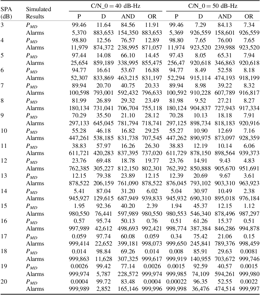
The results are presented in Table 1. For general performance analysis, we assume the threshold for a good performance to be at least 90% of spoof detection, in this case, this can translate at most 10% average P MD . We observe that in the P metric alone, for the spoofer power advantage ranging from 3 dB to 13 dB, the percentage average P MD during lift-off is above 10% with as bad as 99% in 3 dB spoofer power advantage, which only showed 5,370 alarms. Only with spoofer power advantage ranging from 14 dB to 20 dB, the percentage average P MD during lift-off is below 10% with as good as 0.0004% on 20 dB spoofer power advantage which only showed 999,989 alarms.
PMD and alarms for P, D, AND, OR metrics.

Table 1. Long description
A table comparing simulated results for P, D, AND, OR metrics at different SPA levels and C/N_0 values. The table has 20 rows and 8 columns. Columns are labeled SPA (dB), Simulated Results, P, D, AND, OR for C/N_0 = 40 dB-Hz and C/N_0 = 50 dB-Hz. Each row provides values for P_MD and Alarms for the metrics P, D, AND, OR at specific SPA levels. Row 1: SPA 3, P_MD 99.46, Alarms 5,370, P 11.64, D 883,653, AND 154,350, OR 883,653. Row 2: SPA 4, P_MD 98.80, Alarms 11,979, P 12.56, D 874,372, AND 238,995, OR 871,057. Row 3: SPA 5, P_MD 97.44, Alarms 25,654, P 14.08, D 859,189, AND 338,995, OR 855,475. Row 4: SPA 6, P_MD 94.77, Alarms 52,307, P 16.61, D 833,869, AND 463,215, OR 831,197. Row 5: SPA 7, P_MD 89.94, Alarms 100,598, P 20.70, D 793,001, AND 592,432, OR 796,633. Row 6: SPA 8, P_MD 81.99, Alarms 180,134, P 26.89, D 731,041, AND 706,704, OR 755,118. Row 7: SPA 9, P_MD 70.29, Alarms 297,133, P 35.50, D 645,045, AND 781,794, OR 718,741. Row 8: SPA 10, P_MD 55.28, Alarms 447,261, P 46.18, D 538,185, AND 831,738, OR 707,545. Row 9: SPA 11, P_MD 38.83, Alarms 611,721, P 57.97, D 420,283, AND 837,395, OR 737,020. Row 10: SPA 12, P_MD 23.76, Alarms 762,385, P 69.48, D 305,227, AND 812,150, OR 802,301. Row 11: SPA 13, P_MD 12.15, Alarms 878,522, P 79.38, D 206,159, AND 761,090, OR 878,522. Row 12: SPA 14, P_MD 5.41, Alarms 945,927, P 87.04, D 129,615, AND 687,949, OR 939,833. Row 13: SPA 15, P_MD 1.95, Alarms 980,550, P 92.36, D 76,441, AND 597,989, OR 980,550. Row 14: SPA 16, P_MD 0.57, Alarms 997,989, P 95.74, D 42,612, AND 498,693, OR 992,421. Row 15: SPA 17, P_MD 0.059, Alarms 999,414, P 97.74, D 22,652, AND 399,181, OR 998,073. Row 16: SPA 18, P_MD 0.014, Alarms 999,863, P 98.84, D 11,628, AND 307,325, OR 999,617. Row 17: SPA 19, P_MD 0.0026, Alarms 999,974, P 99.42, D 5,787, AND 228,572, OR 999,974. Row 18: SPA 20, P_MD 0.0004, Alarms 999,989, P 99.72, D 2,852, AND 165,146, OR 999,996.
In the D metric alone, for all the spoofer power advantages ranging from 3 dB to 20 dB, none of the percentage average P MD during lift-off fell below 10%. Only with 3 dB SPA did the performance came close to the threshold with 11.64%, while at 20 dB SPA, it is as bad as 99.72% with only 2,852 alarms.
In the AND combination alone, for all the SPA ranging from 3 dB to 20 dB, none of the percentage average P MD during lift-off fell below 10%. Only with 10 dB and 11 dB SPA, the performance came close to the threshold with approximately 16% and approximately 830,000 alerts, while performing worse when diverging to both ends of the range, with 84.56% and 154,350 alarms at 3 dB SPA, and 83.48% with 165,146 alarms at 20 dB SPA.
In the AND combination, the overall better performance is observed with less than 10% average P MD during lift-off from 14 dB to 20 dB with as low as 0.0004% and 999,996 alarms observed at 20 dB SPA. The worst performance peaked at 10 dB SPA with 29.25% and 707,545 alarms, which is still relatively better than the worst of the other gates and metrics. Furthermore, from the worst peak towards the lower SPA, the performance kept getting better with 11.91% and 883,653 alerts at 3 dB SPA, which is close to the 10% threshold.
To get further analysis results of the individual metrics and gate performances, we adjusted other variables and repeated the simulation. Since the nominal GPS receiver
 $C/{N_0}$
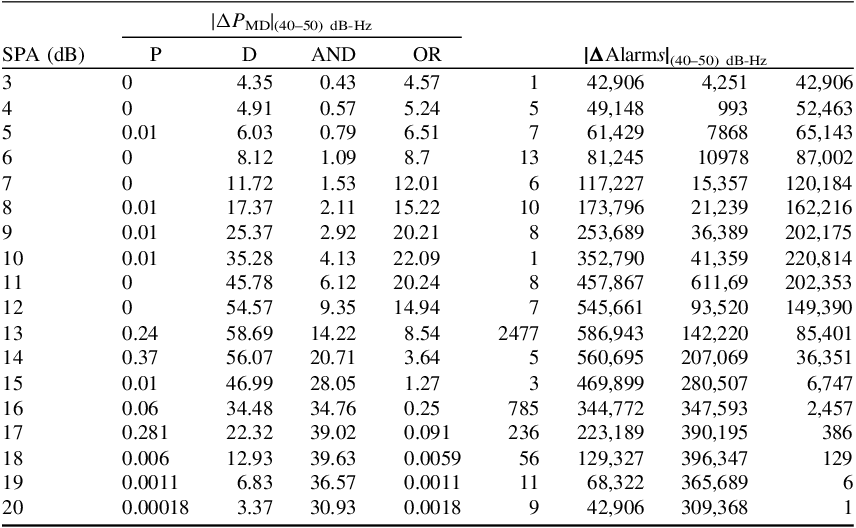
values often are in the 40–50-dB-Hz range, we tried all the values in this range with the same SPA range of 3 dB to 20 dB. We only include the simulation results at 50 dB-Hz. The results are presented in the right half of Table 1. To compare the performance difference at 40 dB-Hz to 50 dB-Hz, from Table 1, we deduce value differences and present the result in Table 2 for percentage average P
MD
and number of alarms differences.
PMD and alarms difference for P, D, AND, OR metrics between C/N0 = 40 and 50 dB-Hz.

Table 2. Long description
A table comparing performance metrics and alarm differences for various signal-to-noise ratios. The table has 18 rows and 9 columns. The columns are labeled as follows: SPA (dB), P, D, AND, OR, and four columns for Alarms with different conditions. Each row provides specific values for these metrics. The table presents data for SPA values ranging from 3 dB to 20 dB. The values in the columns represent different performance metrics and alarm differences at specific signal-to-noise ratios. The table is divided into two main sections: one for PMD values and one for Alarms values, each with different conditions. The data shows variations in performance metrics and alarm differences across different SPA values.
From Table 2, for the P metric, we observe negligible performance change with different
 $C/{N_0}$
values from 40 to 50 dB-Hz. For the D metric, we noticed a very large performance change with as high as 58.69% difference of average P
MD
from 40 to 50 dB-Hz. It can also be observed from Table 1 that 3 dB to 8 dB also fall below the 10% threshold unlike in Table 1, which means the D metric performed better in the case of higher
 $C/{N_0}$
values.
For the AND gate combination, the performance gap is observed to increase from the lower to higher
 $C/{N_0}$
values. The performance was worse at lower
 $C/{N_0}$
, for instance for 40 dB-Hz and 20 dB SPA, the percentage average P
MD
was 83.48%, but got significantly better for 50 dB-Hz with the same 20 dB SPA where the percentage average P
MD
was 52.55%.
For the OR gate combination, the performance gap between these different
 $C/{N_0}$
values is very insignificant on lower and higher SPA values, and a significant change is in the middle range values from 7 dB to 12 dB. The performance was worse in lower
 $C/{N_0}$
, for instance, for 40 dB-Hz and 10 dB SPA, the percentage average P
MD
was 29.25%, but got significantly better for 50 dB-Hz with the same 10 dB SPA, where the percentage average P
MD
was 7.16%.
These observations are crucial in understanding individual metrics with which we will be dealing to find a specific combination arrangement and its performance optimisation in Section 3.
3. Proposed approach: nature of the contribution and design trade-offset
Before detailing the decision framework, it is necessary to establish the theoretical scope of the proposed methodology. The Multilayer Auto Switcher Comparator (MLASC) constitutes an architectural and heuristic engineering solution rather than a strictly derived, statistically optimal detector. Formulating a theoretically optimal joint likelihood test across dynamic, uncooperative spoofing vectors requires real-time resolution of complex, multidimensional probability density functions. Such mathematical rigour, while theoretically ideal, imposes processing overheads that are largely intractable for the resource-constrained firmware of legacy civil aviation GNSS receivers. Consequently, the MLASC framework deliberately trades strict statistical optimality for computational pragmatism. By using combinations of three-input logic gates to route metrics based on the inferred threat regime, the architecture acts as a lightweight, low-latency surrogate. This heuristic approach relies on structural redundancy, via layer swapping and selective metric averaging, to approximate optimal detection bounds while remaining operationally feasible for real-time legacy hardware integration.
3.1. Decision framework
For N metrics that are mutually independent, as shown by Rothmaier et al. (Reference Rothmaier, Chen, Lo and Walter2021), Equation (8) is the optimisation problem for different scenarios, that is, scenario simple
 ${H_0}$
, composite
 ${H_1}$
combined with scenario composite
 ${H_0}$
, simple
 ${H_1}$
or scenario simple
 ${H_0}$
, composite
 ${H_1}$
combined with scenario simple
 ${H_0}$
, simple
 ${H_1}$
by allocating the same
 ${P_{F{A_{max}}}}$
to each monitor,
 $$P\left(\mathop \sum \limits_{n = 1}^N log{\Lambda _m} \lt \;\gamma {\rm{\;|\;}}{H_0}\right) \le {P_{F{A_{max}}}}{\rm{\;}}$$
where Pm,λ(x) is the cumulative density function of the noncentral chi-squared distribution with k degrees of freedom and no centrality parameter λ evaluated at x and
 $C_m^{ - 1}\left( p \right)$
is the inverse χ2 cumulative density function with k degrees of freedom evaluated at p.
Figure 2 describes a three decision guidance for the detector. If there is spoof but no alert, that is a missed detection and if there is an alert but there was no spoof, that is a false alert. The correct detection is when the alert is triggered when a spoofing attack is detected and when no alert is triggered when no spoofing attack is detected.
-
Model assumptions and limitations
Alerts in null and spoofed conditions to determine the correct and incorrect detections.

The MLASC framework is designed as a single-antenna, signal-processing defence mechanism. Consequently, the operational threat model evaluated here is scenario-based, focusing specifically on tracking-points-carry-off attacks during the lift-off phase. During this phase, the interaction between the authentic and counterfeit signals provides the necessary physical overlap to trigger the autocorrelation distortion metric.
This framework does not currently evaluate capability-based attacks such as perfect seamless takeovers using phase-aligned signal nulling. In a perfect nulling scenario, the authentic signal is eliminated, stripping the system of the distortion metric and leaving it reliant solely on power monitoring. Furthermore, defences against spatial-domain spoofing (requiring multi-antenna arrays) and data-level navigation-domain manipulations (requiring downstream PVT cross-checks) are considered out of the scope for this specific framework. MLASC is intended to serve as a highly optimised, firmware-updatable, pre-correlation detection layer within a broader, defence-in-depth receiver architecture.
-
Practical implementation and regime robustness
While Spoofer Power Advantage (SPA) serves as an independent variable for simulation design, true SPA is unobservable in practice; the physical receiver instead triggers the adaptive switching via observable power deviations
 $\sqrt C $
, against a nominal
 $C/{N_0}$
baseline. Near boundary thresholds (e.g. 8 dB), estimation noise introduces risks of regime misclassification. The MLASC framework inherently mitigates this via its final Comparator combination modalities. By blending detection probabilities across multiple layers, the framework prevents single-point boundary failures, ensuring overall detection robustness even under imperfect power regime estimation.
-
Detection-theoretic performance metrics
To maintain strict detection-theoretic rigour and avoid the statistical ambiguities associated with arbitrary threat prevalence, the performance of the MLASC framework is quantified purely via conditional probabilities within the Neyman–Pearson paradigm. Rather than reporting generalised classification accuracy over an arbitrary mix of nominal and spoofed epochs, performance is evaluated via the conditional Probability of Correct Detection (
 ${P_{CD}}$
). By evaluating
 ${P_{CD}}$
(or its complement,
 ${P_{MD}}$
) across a continuous spectrum of SPA values while maintaining a strictly frozen, bounded maximum false alarm configuration, the framework’s sensitivity is mapped directly to the physical threat magnitude. This presentation provides an operationally clear assessment of receiver integrity under worst-case false-alert constraints without requiring an arbitrary assumption of attack prevalence.
3.2. Gate sets and monitors arrangement
The following is a structural hierarchy for the components comprising the MLASC framework.
-
1. Monitors: the foundational algorithmic units that independently calculate specific telemetry metrics (e.g. the Power monitor for P and the Distortion monitor for D)
-
2. Gates: the binary logic operators (AND/OR) that process the threshold outputs of the monitors
-
3. Sets: a specific, hardcoded topological arrangement of gates and monitors. The system uses asymmetric designs, categorised by their dominant logical influence (e.g. an OR-dominant Main Set versus an AND-dominant Minor Set)
-
4. Layer: a complete, independent operational configuration consisting of exactly two complementary Sets (one Main and one Minor) sharing a distributed false-alert budget (
${P_{F{A_{max}}}}$
) -
5. MLASC Framework: the overarching dynamic system that manages multiple parallel Layers, routing logic based on the SPA regime and using a backend Comparator to aggregate the final detection decision.

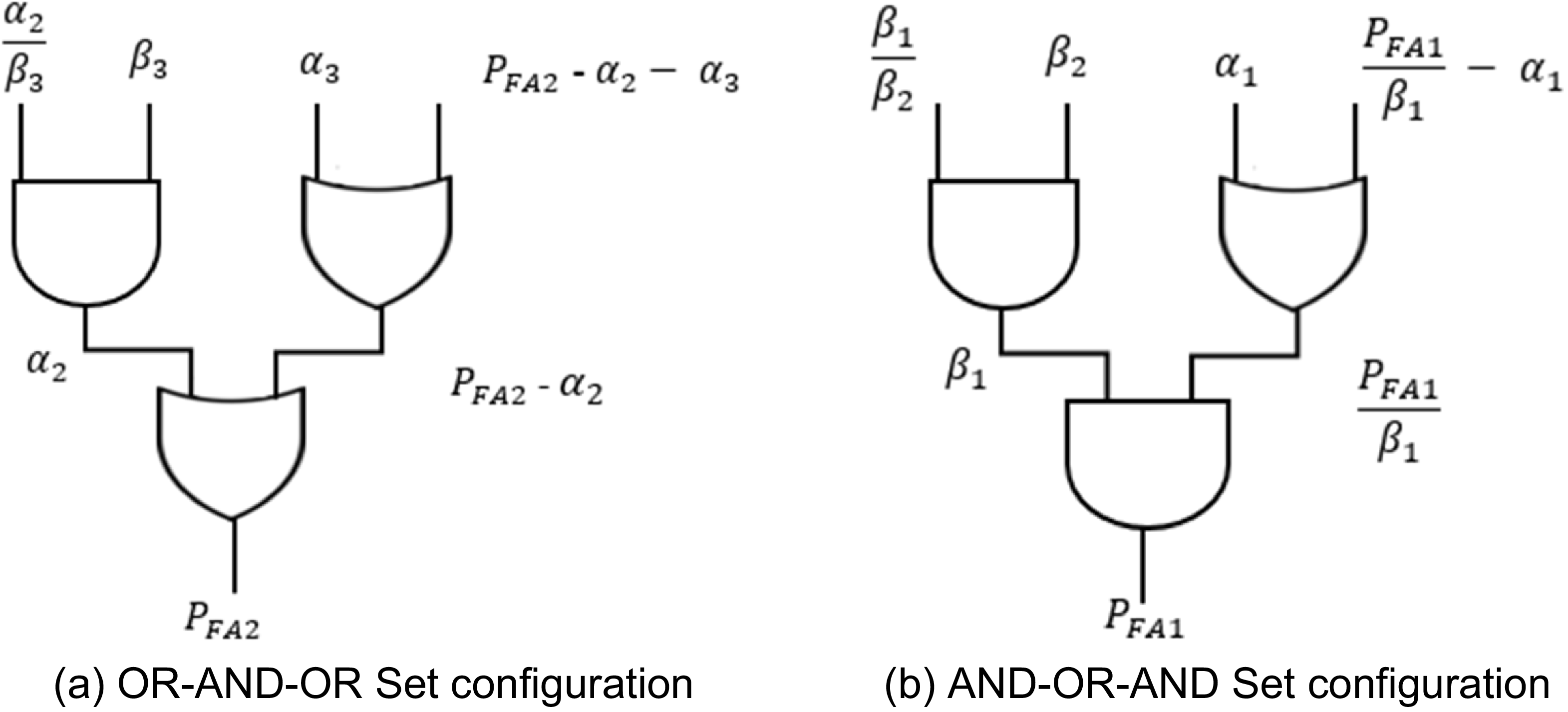
Logic gates come with their caveats such as their susceptibility to transient faults as evaluated by Schvittz et al. (Reference Schvittz, Franco, da Rosa and Butzen2019) and Schvittz et al. (Reference Schvittz, Butzen and Rosa2020). It is crucial to have an effective building block for the overall metric combination. We will intently implement similar principles as the three-input gates for logic synthesis (Marakkalage et al., Reference Marakkalage, Testa, Riener, Mishchenko, Soeken and De Micheli2021) to create sets made of three logic gates for metric combinations. Considering the performance difference of AND gates and OR gates in different scenarios, as briefly analysed in Tables 1 and 2, it is in our best interest to include both in our setup. Since there are scenarios where the AND gate performs better than the OR gate and vice versa, the foundational setup will consist of two sets, one which takes more advantage of the AND gate, while the other capitalises on the OR gate.
Consider three AND gates assigned the budget for the false alert probability as
 ${\beta _1},{\beta _2}{\rm{\;\;}}and{\rm{\;}}{\beta _3},$
and three OR gates assigned the budget for the false alert probability as
 ${\alpha _1}$
,
 ${\alpha _2}$
and
 ${\alpha _3}$
. The first set shown in Figure 3a has two OR gates and one AND gate, which makes the OR gate the dominant one, while the second set in Figure 3b has two AND gates and one OR gate, which makes the AND gate the dominant one.
Logic gates sets: (a) OR-AND-OR set configuration; (b) AND-OR-AND set configuration.

Each set is assigned its own
 ${P_{FA}}$
budget and totals to
 ${P_{F{A_{max}}}}$
as
 $${P_{F{A_{max}}}} = {P_{FA1}} + {P_{FA2}}$$
The designer may distribute the monitors among the two sets based on any of their distinguishing factors, if any, such as, but not limited to, the type or number of metrics each monitor contains.
Based on their contribution to performance of the overall combination involving both sets, the more impactful set is referred to as the Main set and the less impactful as the Minor set. The two sets complete what we refer in this paper to as a layer, discussed further in the next section.
3.3. Multilayer configuration
As shown in the last subsection, monitors that characteristically require their own
 ${P_{FA}}$
budget can be configured into their own sets where they will share a maximum
 ${P_{FA}}$
budget set for them. Here,
 ${P_{FA}}$
for every set is assigned such that the total the
 ${P_{FA}}$
of all the sets of the available monitors is
 ${P_{F{A_{max}}}}$
. This configuration is what forms a single layer, as shown in Figure 4(a).
Due to some factors such as shared error accumulation from monitors in the same set, it is a good practice for the designer to have different sets selection for the same monitor. For instance, hypothetically say there are 8 monitors, 4 for power and 4 for distortion, and the designer put m1, m2, m3 and m4 in the same set to share
 ${P_{FA1}}$
and the rest of the monitors into another set to share the
 ${P_{FA2}}$
due to their similarities. If the monitors m1 and m3 cause higher error accumulation regardless of their similarity, it is logical to try a different sets configuration of such monitors, for instance, swapping m3 with another monitor from the OR-AND-OR SET, hence having m1, m2, m5 and m4 in the same set to share
 ${P_{FA1}}$
and the rest of the monitors into another set to share
 ${P_{FA2}}$
. This will form another layer with its own
 ${P_{F{A_{max}}}}$
.
Per the designer’s analysis of the available monitors, different multiple layers can be configured for the same monitors to form what we refer to here as a multi-layer configuration, which is shown in Figure 4(b). From each layer, the P MD can be deduced and implemented as seems fit.
We suggest a few ways to go about it. First is implementing a comparator to decide which layer configuration performs better in which scenarios, such as spoofer power advantages, and use all the layers interchangeably to the benefit of the anti-spoofer. The second is to get the average of the P MD from all the layers to take advantage of every layer strength contribution in the weakness of the other. The average of all the layers can also be compared with the performance of the individual layers.
Since the combination of both an OR gate and an AND gate into another OR gate, as in Figure 3, has similar output patterns as a standalone OR gate, the
 ${P_{MD}}$
of OR-AND-OR can be deduced using the concept of Equation (3). Similarly, with the combination of an OR gate and an AND gate into another AND gate as in Figure 3b, the
 ${P_{MD}}$
of AND-OR-AND SET can be deduced using the concept of Equation (4).
From Equations (3) and (4), we get
 $${\left( {{P_{MD}}} \right)_{SET1}} = \mathop \prod \limits_{M = n + 1}^N {P_{MD}},n{\rm{\;\;}}$$
 $${\left( {{P_{MD}}} \right)_{SET2}} = 1 - \mathop \prod \limits_{M = 1}^n (1 - {\rm{\;}}{P_{MD}},n){\rm{\;\;}}$$
In a similar manner, the JOINT metric was formed by Rothmaier et al. (Reference Rothmaier, Chen, Lo and Walter2021), and we can deduce the
 ${P_{MD}}$
of each layer in the simplest form as
 $${({P_{MD}})_{LAYER}} = 1 - \;\prod\limits_{m = 1}^n {\left( {1 - \;{P_{k,{\lambda _m}}}\left( {C_m^{ - 1}\left( {1 - {1 \over n}{P_{FA1}}} \right)} \right)} \right)} \; + \prod\limits_{m = n + 1}^N {{P_{k,{\lambda _m}}}} \left( {C_m^{ - 1}\left( {1 - {1 \over {N - n}}{P_{FA2}}} \right)} \right)\;$$
where k is the degree of freedom in the cumulative density function (cdf) and
 ${\lambda _m}$
encodes the metrics in the respective set for different attack scenarios.
In the case of more than one layer, the average of the layers is deduced and the comparator at the end of the two layers can decide the best possible output as we suggested earlier, that is to go with either of the layers or their average. For the number of layers used,
 ${N_L}$
, the average P
MD
is
 $$\eqalign{ & {({P_{MD}})_{AVERAGE}} = {1 \over {{N_L}}}\sum\limits_{Layer = 1}^{{N_L}} {\left(1 - \;\prod\limits_{m = 1}^n {\left( {1 - \;{P_{k,{\lambda _m}}}\left( {C_m^{ - 1}\left( {1 - {1 \over n}{P_{FA1}}} \right)} \right)} \right)} \right.} \cr & \ \ \ \ \ \ \ \ \ \ \ \ \ \ \ \ \ + \prod\limits_{m = n + 1}^N {{P_{k,{\lambda _m}}}} \left.\left( {C_m^{ - 1}\left( {1 - {1 \over {N - n}}{P_{FA2}}} \right)} \right)\right) \cr}$$
3.4. Performance optimisation
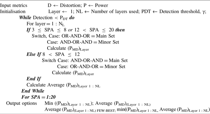
To maximise the efficiency of the monitors and gates in the arrangement within the set and layers, the optimisation is done and summarised in Algorithm 1
. Some of the decisions such as spoofer power advantage set switching within the algorithms are not fixed and can be adjusted depending on the specific scenarios. Based on the number and relationships of the power and distortion metric monitors available, the designer will distribute them into an OR-AND-OR set as described earlier and initialise the resulting number of layers. The detection threshold set in
 $\gamma $
is also initialised. Within the detection threshold, the optimisation of one layer after another begins until the end of all the number of layers used. The reasonable spoofer power advantage is from 3 dB to 20 dB, but the values can be adjusted in the optimisation as seen fit per specific scenarios. Since the P
MD
in any layer is contributed by two sets, one can be considered as the Main Set and another as the Minor Set based on their contribution to performance.
For instance, considering the results of Table 1, the OR gate showed better performance for a lower spoofer power advantage of approximately 3 dB to 8 dB. As described in the previous section, the OR-AND-OR set is the best option as the Main Set because the OR gates are dominant. Switching it as the Main Set in the optimisation process can be implemented in several ways such as accumulating more monitors in this set or assigning it a lower probability of false alerts, PFA, as less false alerts are expected from the Main Set compared with the Minor Set. Then from a medium spoofer power advantage of approximately 8 dB to 12 dB, the AND gate showed better performance. Here, the AND-OR-AND set is the best option as the Main Set since the AND gates are dominant. Switching it as the Main Set in the optimisation process can also be implemented in several ways such as accumulating more monitors in this set or assigning it a lower probability of false alerts, PFA, as less false alerts are expected from the Main Set compared with the Minor Set. Thereafter, the OR gate again showed better performance on a higher spoofer power advantage of approximately 12 dB to 20 dB. The Main Set will be switched to the OR-AND-OR set again, for the same reason and by the same implementation mentioned prior.
MLASC optimisation

Algorithm 1 Long description
An equation describing an algorithm for optimization. The algorithm starts with input metrics for distortion and power. Initialization involves setting the number of layers and detection threshold. A while loop runs until detection is less than the detection threshold. For each layer, if the spoofer power advantage is between 3 and 20, it switches between main and minor sets based on specific conditions. The power of the main distortion is calculated for each layer. The average power of the main distortion across all layers is then calculated. A for loop runs for spoofer power advantage values from 1 to 20. Output options include the minimum and average power of the main distortion across all layers, and the few-best average power of the main distortion.
On every switching, the P MD is calculated from the sets and the final, and after the end of the layer, the P MD is the compilation of those calculated on each set. In this manner, we optimise the use of gates in each set and assure the best possible detection on every scenario. After the first layer results are in, the same step is repeated for every layer until NL and at the end, all average P MD is deduced as Equation (13). Finally, the comparator is used to decide which final P MD should be used as the usable detector result. There are four best ways to go about this. First, the output may be P MD from one of the layers that produced the best results, that is, the overall minimum P MD in different scenarios. Second is the average P MD from all the layers. Third is the average P MD of only the few best performing layers. Fourth is the best among individual layers and their average.
While Algorithm 1
uses power deviation estimates to dictate layer transitions, this dependency is physically required to prevent detection blindness during high-power attacks. During overpowering spoofing scenarios (e.g. SPA > 14), the spoofed signal completely dominates the correlator, causing non-power monitors like the distortion metric (D) to return to a nominal, symmetric state and fail to detect the attack. Therefore, power metrics are strictly necessary to establish the macro-state of the attack environment, while non-power monitors act as complementary threshold drivers primarily within the high-interaction, low-to-medium power domains (
 $3{\rm{\;dB}} \le {\rm{SPA}} \ge 12{\rm{\;dB}}$
).
This proposed method contains the multilayer configuration and auto-switcher comparator as described in this section and we summarise its name as the Multi-layer Auto-switcher Comparator, MLASC, as a spoofing detection technique. The overall multi-layer configuration is shown in Figure 5.
3.4.1. Computational complexity and real-time feasibility
For an anti-spoofing mechanism to be viable for real-time integration into legacy civil aviation GNSS receivers, its computational overhead must be minimal. The MLASC framework achieves this by decoupling its detection logic from the receiver’s high-rate correlator engine. The constituent Power (P) and Distortion (D) metrics are derived directly from standard tracking-loop telemetry (the prompt, early and late correlator accumulation taps), meaning the framework requires no additional signal replication or tracking channels.
The secondary optimisation layer governed by Algorithm 1
and the backend Comparator relies purely on discrete, low-rate algebraic operations. The switching rule consists of basic conditional boundary checks, and the logic gates process binary or scalar probability values. The primary computational expense within the framework lies in the evaluation of the non-central chi-squared cumulative density functions (
 ${P_{k,{\lambda _m}}}$
) and their inverses (
 $C_m^{ - 1}$
) during the
 ${({P_{MD}})_{LAYERS}}$
calculations. For a system configured with
 ${N_L}$
layers, the worst-case computational complexity per tracking epoch is deterministic and scales linearly as O(
 ${N_L}$
). Because
 ${N_L}$
is a small static integer constant (
 ${N_L} = 5$
in this study), the execution requires only a negligible number of clock cycles per epoch. The architecture completely avoids matrix inversions, iterative optimisation algorithms or high-dimensional search grids, rendering it fully compatible with the real-time processing budgets of legacy firmware architectures and standard embedded digital signal processors (DSPs).
4. Simulation results and analysis
For simulation and result analysis of our work, we implement the method given by Rothmaier et al. (Reference Rothmaier, Chen, Lo and Walter2021), which is from where our work expands, and modify it accordingly per this study’s proposed approach. It is necessary to get the best variety of spoofing detection methods and any new or improvement of the previous methods is important since in GNSS, the quality of service is always held at high standards due to its significance. For instance, in civil aviation, according to Eurocae (2023), Novella et al. (Reference Novella, Pena, Macabiau, Martineau, Ladoux, Estival and Troubet-Lacoste2022) and RTCA (2018), the GNSS receivers for aviation applications have an acquisition threshold certification. The current generation of GNSS receivers used in civil aviation are called legacy receivers. This type of receiver exclusively uses GPS L1 C/A signals for location and timing. For position and time, these receivers exclusively use GPS L1 C/A signals.
In our experiment, we simulated data based on standard GPS L1 C/A parameters and use them for spoofing detection performance analysis based on the proposed approach. We simulated 1,000,000 Monte Carlo runs at every 107 epochs with the following parameters:
-
1. nominal signal strength,
$C/{N_0}$
= 40 dB-Hz -
2. spoofer power advantage, SPA = 3 dB to 20 dB
-
3. background noise,
${N_0}$
in Equation (1) is 203 dBW/Hz -
4. early/late correlator positions in chips from prompt, Δτ = 0.052, considering an attack that modifies its code phase at a consistent rate, while maintaining a constant signal strength where the delta metric can only indicate the attack during lift-off if there is a coding phase discrepancy of no more than 1 + chips between genuine and spoof signals
-
5. the Delta metric can only indicate the attack during liftoff if there is a coding phase discrepancy of no more than 1 + Δτ chips between authentic and spoof signals
-
6. budget shared equally among monitors in the OR as well as AND combination case,
${P_{F{A_{max}}}}$
=
${10^{ - 8}}$
-
7. budget shared equally among monitors in the Main Set combination case,
${P_{F{A_{main}}}}$
=
$6 \times {10^{ - 9}}$
-
8. budget shared equally among monitors in the Minor Set combination case,
${P_{F{A_{minor}}}}$
=
$4 \times {10^{ - 9}}$


Some of the parameters such as shared budgets for Main and Minor Sets will be adjusted in the later tests for comparison analysis. All the simulations were run on an 11th Gen Intel(R) Core(TM) i7-1165G7 @ 2.80GHz 2.80 GH 64-bit operating system, x64-based processor, 32.0 GB RAM machine.
The output from the software tool can be displayed in two-dimensional (2D) and three-dimensional (3D) graphs showing the average P MD during lift-off or the alarms at different Spoofer power advantages. Figure 6a shows the 3D planes of individual P and D metrics, and gates AND, OR, Main Set, Minor Set and MLASC combined metrics. Any point selected from the plane will give important information about detection at that point in that particular metric plane. We will isolate and analyse some of the planes individually, a process that can be done easily from the software tool.
Single layer versus multi-layer sets configuration: (a) single layer; (b) multi-layer.

Overall multi-layer configuration.

Figure 5. Long description
A diagram of a multi-layer configuration for spoofing countermeasures. The diagram is divided into three layers: Layer 1, Layer 2, and Layer 3. Each layer contains sets of monitors and logical gates. Layer 1 includes SET 1 and SET 2, each with monitors labeled M1 to Mn and Mn+1 to MN, respectively. These sets feed into logical gates. Layer 2 includes SET 3 and SET 4, similarly structured with monitors and logical gates. The outputs from Layer 1 and Layer 2 are combined and processed in Layer 3, which includes additional logical gates and a final output section labeled with L1, P MD, L1L2, Ave P MD, and L2, P MD. The diagram shows the flow of information through these layers, indicating a hierarchical structure for processing and monitoring signals.
3D planes for performance of multiple metrics, AND gate, OR gate and Minor Sets. (a) The multiple metrics. (b) The AND gate. (c) The OR gate. (d) The Minor Sets within one layer and five layers.

The building blocks for the JOINT combination may be considered to be the AND gate and OR gate, while for the MLASC method are Main Set and Minor Set, which are made of multiple gates.
To compare the performance of these building blocks, first consider the AND gate and OR gate results in Figures 6b and 6c, respectively. It can be observed that the planes provide almost the same results as in Table 1 for both gates.
On a plane at any spoofer power advantage, there are several values for alarms and P MD where the best selection is obtained from the end points of the plane in that particular SPA. One end gives the minimum alarms and the other end gives its corresponding P MD . For instance, for the OR gate in Figure 6c, consider the spoofer power advantage of 10 dB, the alarms at the minimum end of alarms are 707,545 alarms, which is the same value obtained in Table 1, and its P MD is roughly 29.19, which is almost the same as 29.25 in Table 1. As expected, the planes for the AND gate and OR gate produce the same results as Table 1 in a more insightful visualisation manner.
The performance of the Minor Set alone shows satisfactory performance from a configuration with only one layer and gets better in configuration with higher number of layers as it can be observed from Figure 6d showing the 3D planes for detection performance of the Minor Sets in a configuration with one layer versus a configuration with four layers. Consider SPA of 3 dB, the P MD of 0.036 is achieved in four-layer configuration compared with 0.103 in the one-layer configuration and 963,596 alarms in the four-layer configuration compared with the 897,727 in the one-layer configuration.
The performance of the Main Set also shows satisfactory performance from a configuration with only one layer and gets better in configuration with higher number of layers as it can be observed from Figure 7a showing the 3D planes for detection performance of the Main Sets in a configuration with one layer versus a configuration with four layers. The comparison of the main and Minor Sets P MD and alarms performance in a one-layer configuration can be observed in Figures 7b and7c.
PMD versus alarms for Main and Minor Sets. (a) The 3D planes for performance of Main Sets within a one layer and a five-layers configuration. (b) PMD. (c) Alarms.

Figure 7. Long description
The image contains three panels. Panel A shows a 3D surface plot illustrating the performance of main sets within a one-layer and a five-layers configuration. The x-axis represents the number of alarms, the y-axis represents the spoofing power advantage (SPA) in decibels (dB), and the z-axis represents the missed detection probability. The plot includes multiple layers, each with different colors, indicating varying detection probabilities. Panel B is a line graph showing the average probability of missed detection (P_MD) during lift-off in percent on the y-axis versus the spoofer power advantage in dB on the x-axis. Two lines are plotted: one for the minor set (blue dashed line) and one for the main set (orange dashed line). The minor set line shows a decreasing trend, while the main set line shows a more stable trend. Panel C is another line graph depicting the number of alarms on the y-axis versus the spoofer power advantage in dB on the x-axis. Again, two lines are plotted: one for the minor set (blue dashed line) and one for the main set (orange dashed line). The minor set line shows an increasing trend, while the main set line shows a more stable trend.
The main and Minor Sets are proven to be better building blocks than the individual gates and their performance is compared in Figures 8a and 8b.
Results of PMD and alarms using different methods. (a) PMD for Main and Minor Sets versus AND and OR gate. (b) Alarms for Main and Minor Sets versus AND and OR gate. (c) PMD for Main versus Minor Sets and MLASC versus JOINT. (d) Alarms for Main versus Minor Sets and MLASC versus JOINT.

Take SPA of 3 dB for instance, the Minor Set in one layer configuration raises 897,727 alarms compared with 88,099 and only 15,429 for the AND gate and OR gate, respectively, and has P MD of 0.103 compared with 0.119 and 0.846 for the AND gate and OR gate, respectively.
The OR gate is observed to have a slightly better performance from SPA of approximately 15 dB to 20 dB; however, the gap is closed and OR is outperformed when having configuration with a higher number of layers.
This performance observed from the AND gate and OR gate, as well as the Main and Minor Sets as building blocks, is carried over to their resulting combinations, that is, the JOINT combination and MLASC, respectively, and their performance is compared in Figures 8c, 8d and 9.
3D planes for MLASC with different number of layers. (a) MLASC with different number of layers. (b) MLASC with only one layer versus with five layers.

Figure 9. Long description
Panel A: A 3D plane graph titled ‘MLASC with different number of layers’ shows the relationship between missed detection probability, signal-to-power ratio (SPA) in decibels, and the number of alarms. The x-axis represents the number of alarms, the y-axis represents the signal-to-power ratio (SPA) in decibels, and the z-axis represents the missed detection probability. The graph includes multiple data points labeled with different configurations such as ‘JOINT’, ‘SPA (dB) 3’, and ‘MLASC - L5’, each with corresponding values for alarms and probability of missed detection (PMD). The color gradient from blue to red indicates increasing detection probability. Panel B: Another 3D plane graph titled ‘MLASC with only one layer vs. with 5 layers’ compares the missed detection probability for configurations with one layer and five layers. The x-axis represents the number of alarms, the y-axis represents the signal-to-power ratio (SPA) in decibels, and the z-axis represents the missed detection probability. The graph shows two distinct surfaces labeled ‘MLASC - L1’ and ‘MLASC - L5’, with a color gradient from blue to red indicating increasing detection probability.
The MLASC method implementing only one layer performs better than the JOINT method especially for the SPA from 3 dB to 15 dB. Taking 7 dB, for instance, the MLASC has the average P MD of 6.54% compared with a JOINT combination of 10.37%. This difference is significant especially if we are set to achieve at least 90% detection. At higher SPA from 15 dB to 20 dB, the JOINT method slightly outperforms the MLASC, for instance, with 17 dB SPA, the P MD of 1.266% for MLASC is achieved compared with 0.199% in JOINT combination. This difference is very small and the performance of both methods can be considered good enough in high SPA values.
As the MLASC is configured with higher number of layers, the gap in performance difference between the MLASC and JOINT at higher SPA values shrinks more while it expands more at lower SPA values. This means the overall performance of the MLASC is getting better if it is configured with more layers, while the JOINT method remains the same. Figure 9b shows the 3D planes for MLASC with only one layer compared with the other configured with 5 layers using the same PFA1 and PFA2 distribution in each layer. The number of alarms and P MD between the two shows how more layers mean better performance.
What determines whether or not to use more than one layer if there is a different configuration compared with the first layer, with a potential of improving performance? We consider the MLASC method implemented by one layer to five layers configuration using the same PFA1 and PFA2 distribution, and presented their the P MD results in Figure 10a and they can be compared with the JOINT combination. As observed in their 3D planes, below 15 dB SPA, the gap between the JOINT and MLASC increases with the number of layers, while above 15 dB SPA, the gap decreases. The overall performance of MLASC is excellent especially with higher number of layer configurations, while in comparison, the JOINT performs excellently at higher SPA values and less at lower SPA values.
PMD for JOINT versus MLASC with different number of layers. (a) JOINT versus MLASC with different number of layers. (b) MLASC with different shared PFA values.

Different PFA1 and PFA2 distributions can also be set differently in each layer. To analyse their impact on the performance, the parameters were also adjusted to analyse the change in PFA budgets share among the sets. The overall findings show the better MLASC performance is obtained when the Main Set has more PFA budget than the Minor set, which is an expected finding. Since the
 ${P_{F{A_{max}}}}$
is set to
 ${10^{ - 8}}$
, we can distribute it between the two sets in 90%–10%, 50%–50% and 10%–90% based on Equation (9).
For instance, for the first case of 90%–10%:
-
1. the budget shared equally among monitors in the OR as well as AND combination case,
${P_{F{A_{max}}}}$
=
${10^{ - 8}}$
-
2. the budget shared equally among monitors in the Main Set combination case,
${P_{F{A_{main}}}}$
=
$9 \times {10^{ - 9}}$
-
3. the budget shared equally among monitors in the Minor Set combination case,
${P_{F{A_{minor}}}}$
=
${10^{ - 9}}$


As observed in Figure 10b, the MLASC performance is better when the Main Set takes 90% of the
 ${P_{F{A_{max}}}}$
, while the Minor Set takes 10%. The performance keeps dropping as more budget share is assigned to the Minor Set. The
 ${P_{F{A_{max}}}}$
budget is to be shared strategically among the sets within each layer based on its monitors to maximise the overall MLASC performance.
The parameters were adjusted testing different
 $C/{N_0}$
from 40 dB-Hz to 50 dB-Hz and the performance discrepancy of MLASC was minimal for their individual results to be presented here.
As demonstrated in Table 3, extracting discrete operational points from the continuous simulation landscape highlights the clear quantitative advantage of the proposed MLASC architecture. At the critical tracking-point-carry-off transition boundaries (particularly between 4 dB and 12 dB SPA), single-gate baselines exhibit severe performance asymmetries, where the OR gate degrades at mid-range power profiles and the AND gate suffers at lower advantages. While the legacy JOINT combination partially smooths these vulnerabilities, the MLASC framework dynamically switches between optimal sub-set topologies across parallel layers. This architectural flexibility yields a lower probability of missed detection (
 ${P_{MD}}$
) across the entire gradient, bridging the performance gaps inherent to traditional fixed-logic structures.
Quantitative comparison of missed detection probability (
 ${P_{MD}}\% $
) (evaluated at a fixed
 ${P_{F{A_{max}}}}$
=
 ${10^{ - 8}}$
under nominal
 $C/{N_0}$
= 40 dB-Hz).

Table 3. Long description
A table comparing the performance of different gates and architectures at various SPA levels. The table has 4 rows and 5 columns. The columns are labeled SPA level (dB), OR gate (%), AND gate (%), JOINT (%), and MLASC (5 layers) (%). The rows are labeled with SPA levels 4, 8, 12, and 16. Row 1: SPA level, 4; OR gate, 12.89 percent; AND gate, 76.57 percent; JOINT, 10.683 percent; MLASC (5 layers), 2.73 percent. Row 2: SPA level, 8; OR gate, 23.49 percent; AND gate, 29.32 percent; JOINT, 9.878 percent; MLASC (5 layers), 0.852 percent. Row 3: SPA level, 12; OR gate, 19.77 percent; AND gate, 18.78 percent; JOINT, 4.193 percent; MLASC (5 layers), 0.582 percent. Row 4: SPA level, 16; OR gate, 0.51 percent; AND gate, 50.13 percent; JOINT, 0.201 percent; MLASC (5 layers), 0.539 percent.
4.1. Framework generalisation and parameter calibration
To ensure the proposed framework is robust and not overfitted to the specific simulation parameters used in this study, it is important to distinguish between the generalised architecture of the MLASC and its calibrated thresholds. The adaptive switching rules defined in Algorithm 1 , specifically the transition to OR-dominant sets at boundary SPA regimes and AND-dominant sets in the mid-power regime, are not merely statistical artefacts of the simulation grid. Rather, they reflect the deterministic physical behaviour of spoofing interactions, where single-metric dominance occurs at power extremes and metric ambiguity occurs during mid-power signal overlap. Consequently, architectural routing generalises across different operational bounds.
The framework’s ability to generalise was verified by evaluating performance across varying nominal carrier-to-noise ratios (
 $C/{N_0}$
ranging from 40 to 50 dB-Hz). As demonstrated in Table 2, while individual constituent metrics experienced significant performance volatility across varying noise floors, the MLASC framework maintained cohesive detection accuracy. It is acknowledged that in practical physical deployment, the specific numeric switching boundaries (e.g. 8 dB and 12 dB) and
 ${P_{FA}}$
budget splits are not universally static. They function as tuneable receiver parameters that a manufacturer would calibrate offline based on the specific thermal noise floor, integration time and front-end characteristics of the target hardware.
5. Conclusion
This work improves the spoofing detection technique using a combination of power and distortion metrics through a special metrics configuration. We analysed the framework used in the previous related approach and used it as a foundation for the new approach. We proposed a multi-metric combination system made of layers, each configured to take advantage of multiple logic gates grouped in two sets where different metric monitors are connected to ensure the minimised probability of missed detections and consequently maximise the probability of correct spoof detection during the attack. The method is also optimised through an auto switcher of the sets, which are the building blocks of the layer, in a way that assures the maximum detection capability in different spoof attack scenarios. The implementation of the proposed technique is illustrated through the development of a spoof detection software tool. The experiment results show a significant leap in spoofing detection compared with the previous frameworks. The practical application may require further development to integrate the software into a particular device for monitoring. While this study establishes the theoretical viability and optimal detection boundaries of the MLASC architecture through high-fidelity Monte Carlo simulations, practical implementation introduces additional physical complexities. Real-world environments contain unmodelled multipath interference and uncalibrated front-end receiver noise that inherently couple with the spoofer’s power profile. Therefore, future work will focus on hardware-in-the-loop (HWIL) testing using physical Intermediate Frequency (IF) datasets and multi-ray fading channels. This will evaluate the framework’s robustness against real-world latent variables and validate the adaptive switching logic under dynamic, physical spoofing conditions.
Acknowledgements
Research for this paper is supported in part by the aviation science foundation of China (201908052002). The authors also gratefully acknowledge the helpful comments and suggestions of the reviewers, which have improved the presentation.





 PMD%
 PFAmax
 10−8
 C/N0


