2.1. Numerical method

The configuration used in this study is an open-channel as depicted in figure 1. It is comprised of a bulk flow region with height $\delta$ and a porous substrate region of depth $h$. The direct numerical simulations using this set-up were conducted using the open-source solver PARIS simulator (Aniszewski et al. Reference Aniszewski2021) with in-house modifications. The code solves the incompressible Navier–Stokes equations,

(2.1a)$$\begin{gather} \boldsymbol{\nabla}\boldsymbol{\cdot}{\boldsymbol{u}} = 0, \end{gather}$$

(2.1b)$$\begin{gather}\frac{\partial \boldsymbol{u}}{ \partial t} + \left(\boldsymbol{u}\boldsymbol{\cdot}\boldsymbol{\nabla}\right){\boldsymbol{u}} =-\frac{1}{\rho}\boldsymbol{\nabla}{p} + \nu{\nabla}^2{\boldsymbol{u}}, \end{gather}$$

where $\boldsymbol {u} = (u,v,w)$, $p$ and $\nu$ are the velocity vector, pressure and kinematic viscosity, respectively. The velocity can be decomposed into its mean and fluctuating components through the Reynolds decomposition (Reynolds Reference Reynolds1895)

(2.2)\begin{equation} {\boldsymbol{u}(x,y,z,t)=\boldsymbol{U}(y)+\boldsymbol{u^{\prime}}(x,y,z,t), } \end{equation}

where $\boldsymbol {u}$ is the instantaneous velocity vector, $\boldsymbol {U}$ is the time- and plane-averaged mean velocity and $\boldsymbol {u^{\prime }}$ is the fluctuating velocity varying over both space and time. Later on in this paper when examining the modulated flow inside the porous substrates, the further decomposition of $\boldsymbol {u^{\prime }}$ into a time-steady and time-varying component (Reynolds & Hussain Reference Reynolds and Hussain1972)

(2.3)\begin{equation} {\boldsymbol{u^{\prime}}(x,y,z,t)=\boldsymbol{\tilde{u}}(x,y,z)+\boldsymbol{u^{\prime\prime}}(x,y,z,t)} \end{equation}

will also be used.

Figure 1.

Sketch of the computational domain.

The dimensions of the computational domain are $(L_x,L_y,L_z)=(6.3\delta,1.3\delta,3.15\delta )$ in the streamwise ($x$), wall-normal ($\,y$) and spanwise ($z$) directions. The domain is periodic along $x$ and $z$ while being bounded by a free-slip surface at $y=\delta$ and a no-slip wall at ${y=-0.3\delta}$. The thickness of the porous substrate is $h=0.3\delta$. The simulations were conducted at a constant mass flow rate, which was adjusted to target a nominal ${Re_{\tau }={u_{\tau }\,{\delta }}/{\nu }=360}$. Here, $u_{\tau }=\sqrt {{\tau _{w}}/{\rho }}$ is the friction velocity at $y=0$ (the substrate surface), with $\tau _{w}$ obtained from the integral balance

(2.4)\begin{equation} {\tau_{w} =-{P_x}\delta,} \end{equation}

where $P_x$ is the mean pressure gradient. Note that at $y=0$, due to presence of a permeable surface $\tau _{w}$ will have contributions from both viscous and turbulent stresses,

(2.5)\begin{equation} {\tau_{w} = \left.{{\mu}\frac{{\rm d}U}{{\rm d} y}}\right\rvert_{y=0} + {{\rho}{\overline{{u^\prime}{v^\prime}}}}\rvert_{y=0}.} \end{equation}

Throughout this paper, the superscript ‘$+$’ indicates scaling in inner units, where quantities are normalized using $u_{\tau }$ and $\nu$. The numerical grid has a resolution of $(N_x,N_y,N_z)=(1620, 324, 810)$. The grid spacing is uniform along $x$ and $z$ while being non-uniform along $y$. The grid is stretched in the region above the substrate using a hyperbolic tangent function and uniform within the substrate. The simulation results are grid independent at the chosen resolution. The grid independence was determined by conducting simulations at coarser and finer resolutions. The results of these simulations are gathered in Appendix A.

The equations are spatially discretized on a staggered Cartesian grid using central second-order finite differences. The fractional-step method (Kim & Moin Reference Kim and Moin1985) is used to solve the discretized incompressible Navier–Stokes equations. At each time step an intermediate non-divergence free velocity field is first calculated. The Poisson equation obtained by imposing the incompressibility constraint is then solved using the fast-Fourier-transform-based solver of Costa (Reference Costa2018) to obtain the pressure correction. The pressure correction is then used to project the velocity field onto a divergence free vector space. The time integration uses a triple-substep Runge–Kutta method where both the advective and diffusive terms are treated explicitly.

The immersed boundary method of Breugem & Boersma (Reference Breugem and Boersma2005) is used to numerically realize the porous substrates. Unlike direct-forcing or penalization-based methods, it involves modifying the discretized advective and diffusive flux terms of the Navier–Stokes equations such that the no-slip and no-penetration conditions become exactly imposed for the regions of the numerical domain which are defined as solids. This makes it a more accurate method for realizing geometries which are Cartesian conforming, as demonstrated by Paravento, Pourquie & Boersma (Reference Paravento, Pourquie and Boersma2008).

In addition to the simulations including porous substrates, an open-channel flow over a smooth wall at $Re_{\tau }=360$ was also simulated to serve as a baseline for comparisons. Quantities normalized using the smooth-wall friction velocity and kinematic viscosity are indicated by the subscript ‘$o$’.

2.2. Porous geometries

The porous substrates investigated are lattices where the pores are repeating rectangular cuboids (figure 2). The solid matrix is made of rods with a cross-section of $d \times d$. The spacings (pitches) $s_x$, $s_y$ and $s_z$ determine the cross-sections of the pores and their resulting void volume. Consistent with previous experimental and numerical studies (Manes et al. Reference Manes, Poggi and Ridolfi2011; Kuwata & Suga Reference Kuwata and Suga2017; Gómez-de Segura & García-Mayoral Reference Gómez-de Segura and García-Mayoral2019), the substrates are characterized in terms of their permeabilities obtained from Darcy's law (Darcy Reference Darcy1856),

(2.6)\begin{equation} {\boldsymbol{u}_D} =-\frac{1}{\mu}{{{\boldsymbol{\mathsf{K}}}}}\boldsymbol{\cdot}\boldsymbol{\nabla}{p}, \end{equation}

where ${\boldsymbol {u}_D}$ is the Darcy velocity vector, ${p}$ is the pressure averaged over the fluid phase and ${{\boldsymbol{\mathsf{K}}}}$ is the permeability tensor. As such, the law represents the balance between the pressure gradient that drives the flow through a porous medium and the resistance exerted by the medium's solid structure upon the flow. As the Darcy permeabilities are only dependent on the geometry of a substrate, they are suitable parameters for encapsulating the geometrical differences between different porous media. Similar to porous structures studied by Kuwata & Suga (Reference Kuwata and Suga2017), the Cartesian structure of the substrates makes the off-diagonal terms of the permeability tensor zero, giving a tensor with only the three diagonal components ${\mathsf{K}}_{xx}$, ${\mathsf{K}}_{yy}$ and ${\mathsf{K}}_{zz}$, which are written as ${\mathsf{K}}_x$, ${\mathsf{K}}_y$ and ${\mathsf{K}}_z$ for simplicity. These components were computed from the results of Stokes flow simulations conducted using representative element volumes (REVs) of each substrate using the same solver that was used for the turbulent flow simulations. The dimensions of the REVs were $(L_x,L_y,L_z)=(0.3\delta,0.3\delta,0.3\delta )$ and the grid resolution similar to the turbulent simulations in terms of grid spacing. The inner-scaled lengths $\sqrt {{{\mathsf{K}}_x}^+}$, $\sqrt {{{\mathsf{K}}_y}^+}$ and $\sqrt {{{\mathsf{K}}_z}^+}$ are used to characterize the porous substrates throughout the paper.

Figure 2.

(a) Schematic of general substrate geometry along with (b,c) its nomenclature.

The main cases (${\rm HP}1$, ${\rm HP}2$, ${\rm HP}3$, ${\rm MP}$, ${\rm LP}1$, ${\rm LP}2$, ${\rm LP}3$) span a range of wall-normal permeabilities, $\sqrt {{{\mathsf{K}}_y}^+}$, to facilitate investigating how near-wall turbulence becomes altered due to a progressively weakening wall-impedance. Here, ${\rm HP}$ designates higher permeability substrates $(\sqrt {{{\mathsf{K}}_y}^+}>2)$, ${\rm LP}$ designates lower permeability substrates $\left (\sqrt {{{\mathsf{K}}_y}^+}<1\right )$ and ${\rm MP}$ a moderate permeability case falling between the other two groups $\Big(1<\sqrt {{{\mathsf{K}}_y}^+}<2\Big)$. Cases ${\rm HP}2'$ and ${\rm HP}3'$ – where the wall-parallel spacings of ${\rm HP}2$ and ${\rm HP}3$ have been swapped – retain the wall-normal permeability of ${\rm HP}2$ and ${\rm HP}3$ but have increased streamwise permeability and hence anisotropy, $\varPhi _{xy}={\mathsf{K}}_x/{\mathsf{K}}_y$.

The simulation parameters along with the characteristics of their porous substrates are gathered in table 1. Representative elements for the ${\rm HP}$ and ${\rm LP}$ porous geometries examined are shown in figure 3. The substrates will first be assessed with regards to certain aspects of permeable-wall turbulence which have been reported in the literature. This includes the transition of turbulence from the canonical near-wall regime to the K–H-like regime (Gómez-de Segura & García-Mayoral Reference Gómez-de Segura and García-Mayoral2019) and the resulting drag changes. An important difference exists between pore-scale resolving simulations, and other simulation approaches such as volume-averaged Navier–Stokes simulations (Breugem et al. Reference Breugem, Boersma and Uittenbogaard2006; Rosti, Brandt & Pinelli Reference Rosti, Brandt and Pinelli2018) and permeable-wall boundary conditions (Jiménez et al. Reference Jiménez, Uhlmann, Pinelli and Kawahara2001; Gómez-de Segura & García-Mayoral Reference Gómez-de Segura and García-Mayoral2019). In the latter approaches, the permeability and porosity are predefined numerical parameters and independent from one another.

Table 1.

The DNS cases of open-channel turbulent flow over porous substrates. The porosity for each substrate is given by $\varphi$. The pore spacings are ${s_{x_o}}^+$, ${s_{y_o}}^+$ and ${s_{z_o}}^+$, while ${\sqrt {{{\mathsf{K}}_{x_o}}^+}}$, ${\sqrt {{{\mathsf{K}}_{y_o}}^+}}$ and ${\sqrt {{{\mathsf{K}}_{z_o}}^+}}$ are the effective permeabilities, which are analogous to the permeability Reynolds number, $Re_{K}$. The ratio of streamwise to wall-normal permeability is ${\varPhi _{xy}}$. The rod or filament thickness of the solid matrix is $d/\delta ={0.039}$ or ${d_{o}}^+={14}$ for all cases. Labels, colours and symbols remain consistent throughout the manuscript.

Figure 3.

Representative elements of the ${\rm LP}$ and ${\rm HP}$ substrates in table 1. (a) ${\rm HP}1$; (b) ${\rm HP}2$; (c) ${\rm HP}3$; (d) ${\rm LP}1$; (e) ${\rm LP}2$; ( f) ${\rm LP}3$. Cases ${\rm HP}2'$ and ${\rm HP}3'$ (not shown) are rotated versions of ${\rm HP}2$ and ${\rm HP}3$ around the $y$ axis by ${\rm \pi} /2$.

For the cases considered in this work, the substrate's geometry determines both the permeability and the porosity. This imposes constraints on the permeabilities and the degree of anisotropy that can be obtained. For example, a change in $s_x$ will change the pore cross-section along both $y$ and $z$, leading to changes in ${\mathsf{K}}_y$ and ${\mathsf{K}}_z$. The Reynolds numbers of DNS studies are also generally low relative to experiments. As such, achieving effective permeabilities $(\sqrt {{{\mathsf{K}}_x}^+}, \sqrt {{{\mathsf{K}}_y}^+}, \sqrt {{{\mathsf{K}}_z}^+})$ which are large (such as those in Manes et al. (Reference Manes, Poggi and Ridolfi2011)) becomes challenging.

3.1. Surface region flow

The changes in the overlying turbulent flow are first assessed qualitatively by examining the flow field above the permeable surface at $y^+\approx 5$. Figure 4 shows instantaneous snapshots of the velocity and pressure fluctuations for ${\rm HP}1$ and ${\rm LP}1$. These two cases have the highest $\sqrt {{{\mathsf{K}}_y}^+}$ of the ${\rm HP}$ and ${\rm LP}$ groups, respectively. This allows for a better assessment of the role wall impedance plays in causing changes in turbulence near the surface. Note that at the surface, the relevant permeability component is ${{\mathsf{K}}_y}$ as the flow must first be able to penetrate into the substrate before becoming redirected into the horizontal directions, for which ${{\mathsf{K}}_x}$ and ${{\mathsf{K}}_z}$ are important.

Figure 4.

Instantaneous (a–c) streamwise velocity, (d–f) wall-normal velocity and (g–i) pressure fluctuations at $y^+\approx 5$: (a,d,g) ${\rm HP}1$; (b,e,h) ${\rm LP}1$; (c, f,i) smooth-wall. Flow direction is from left to right.

Beginning with observations for the streamwise velocity component, ${\rm LP}1$ (figure 4b) exhibits regions of elongated positive and negative fluctuations which are similar to the streaky pattern observed over a smooth-wall (figure 4c). This streamwise coherency is diminished in ${\rm HP}1$ (figure 4a), where the aforementioned regions are instead more clump-like and also exhibit a degree of regularity along the spanwise dimension of the domain. This is indicative of the near-wall turbulence becoming altered. For the wall-normal velocity component, the similarity between ${\rm LP}1$ (figure 4e) and the smooth-wall (figure 4f) is reflective of the similarity seen in their streamwise velocity fields. Case ${\rm LP}1$ has a greater degree of intensity but remains structurally similar to its smooth-wall counterpart; ${\rm HP}1$ (figure 4d), however, shows not only a noticeably stronger intensity in wall-normal velocity fluctuations but also structural differences, with there seemingly being an emergent spanwise coherency. The differences in the pressure fields are consistent with the observations made for the velocity fields. Case ${\rm HP}1$ (figure 4g) demonstrates a spanwise patch along $x^+\approx 1200$ which is coincident with the spanwise coherent regions seen at the same position in its $u$ and $v$ fields. The pressure fluctuations of ${\rm HP}1$ are also more intense compared with ${\rm LP}1$ (figure 4h) and the smooth-wall case (figure 4i). Another distinctive quality of ${\rm HP}1$ is the visible signature of the permeable surface in its flow field, particularly when examining the wall-normal velocity (figure 4d). This indicates that the surface granularity becomes perceived by the turbulent flow, such that it leaves a visible footprint in the flow field. This is similar to what has been observed in flows over roughness (Abderrahaman-Elena, Fairhall & García-Mayoral Reference Abderrahaman-Elena, Fairhall and García-Mayoral2019) and canopies (Sharma & García-Mayoral Reference Sharma and García-Mayoral2020).

3.2. Changes in mean flow, velocity fluctuations and Reynolds shear stress

Surfaces which depart from a hydrodynamically smooth behaviour change the overall level of momentum carried by the bulk flow, i.e. the amount of drag generated at the surface changes. As explained by Spalart & McLean (Reference Spalart and McLean2011) and Chung et al. (Reference Chung, Hutchins, Schultz and Flack2021), a suitable metric for quantifying this is the shift in the logarithmic region of the mean velocity profile, $\Delta {U^+}$, which was introduced by Hama (Reference Hama1954) and Clauser (Reference Clauser1954) and is more commonly known as the roughness function. As such, $\Delta {U^+}$ accounts for the mean momentum deficit of the flow relative to smooth-wall flow. For the porous substrates, this is examined in figure 5(a,b), showing the mean velocity profiles, ${U^+}(y^+)$, and the velocity difference, $\Delta {U^+}(y^+) = {U^+}(y^+)_{{porous}} - {U^+}(y^+)_{{smooth}}$, respectively. All of the porous substrates examined increase drag compared with the baseline smooth-wall case ($\Delta {U^+}<0$), although the ${\rm LP}$ cases do not impose a significant drag penalty. The structural differences observed in the flow over the different substrates are also reflected here, such that they become distinguishable into two overall groups. The substrates with lower wall-normal permeability (${\rm LP}1$, ${\rm LP}2$, ${\rm LP}3$, ${\rm MP}$) do not deviate greatly from the smooth-wall ($\Delta {U^+}>-1$) and the ${\rm LP}$ cases are almost indistinguishable from the smooth-wall case. The substrates with higher wall-normal permeability (${\rm HP}1$, ${\rm HP}2$, ${\rm HP}2'$, ${\rm HP}3$, ${\rm HP}3'$) on the other hand result in $\Delta {U^+}$ values which are notable ($\Delta {U^+}\lessapprox -2$). The same distinction can be made for the Reynolds shear stress (figure 6), where substrates ${\rm LP}1$, ${\rm LP}2$, ${\rm LP}3$ and ${\rm MP}$ result in slightly greater levels of turbulent activity close to the permeable surface whereas this activity is more pronounced for the ${\rm HP}$ substrates with a gap emerging between the former and the latter substrates in terms of their surface-level $-\overline {u^{\prime }v^{\prime }}^+$ activity.

Figure 5.

(a) Mean velocity profiles of the bulk flow region above the porous substrates. (b) Difference in porous-wall and smooth-wall velocities. Symbols and colours follow the descriptions in table 1. The black line in (a) is a reference smooth-wall solution at $Re_{\tau }=360$.

Figure 6.

Reynolds shear-stress profiles of the bulk flow region above the porous substrates. The black line is a reference smooth-wall solution at $Re_{\tau }=360$.

Following the approach of MacDonald et al. (Reference MacDonald, Chan, Chung, Hutchins and Ooi2016) and García-Mayoral, Gómez-de Segura & Fairhall (Reference García-Mayoral, Gómez-de Segura and Fairhall2019), to assess the contributing factors to $\Delta {U^+}$, the mean momentum equation for the bulk flow region above the substrate is considered

(3.1)\begin{equation} {\nu\frac{{\rm d}U}{{\rm d} y}}-\overline{u'v'} = {{u^2_{\tau}}}\left (1 - \frac{y}{\delta}\right ). \end{equation}

Scaling (3.1) in inner units gives

(3.2)\begin{equation} {\frac{{\rm d}U^+}{{{\rm d}y}^+}}-{\overline{u'v'}}^{\,+} = 1 - \frac{y^+}{\delta^+}. \end{equation}

Integrating (3.2) between $y^+=0$ (the substrate surface) and a position far above the substrate where the flow statistics are smooth-wall-like, $y^+=H^+$, results in

(3.3)\begin{equation} \int_{y^+= 0}^{y^+= H^+} -{\overline{u'v'}}^{\,+} \,{{\rm d} y}^++ {U^+}\left(y^+=H^+\right)- {U^+}\left(y^+=0\right) = H^+- \frac{{H^+}^2}{2\delta^+}. \end{equation}

For a smooth-wall flow, there will be no mean velocity at $y^+=0$ (no-slip) and hence ${U^+}(y^+=0)={U^+}_{{slip}}=0$. Taking the difference of (3.3) between a porous case and the smooth-wall case allows for quantifying the contributions of the interfacial slip velocity and changes in Reynolds stress to $\Delta {U^+}$,

(3.4) \begin{align} \Delta{U^+} &= {U^+}\left(y^+=H^+\right)_{{porous}} - {U^+}\left(y^+=H^+\right)_{{smooth}}\nonumber\\ & = U^+_{{slip}} - \int_{y^+= 0}^{y^+= H^+} \left[\left(-{\overline{u'v'}}^{\,+}_{{porous}}\right) - \left(-{\overline{u'v'}}^{\,+}_{{smooth}}\right)\right]\,{{\rm d} y}^+\nonumber\\ &\quad - \frac{{H^+}^2}{2}\left(\frac{1}{{\delta^+}_{{porous}}} - \frac{1}{{\delta^+}_{{smooth}}}\right)\nonumber\\ &= \Delta{U^+_{{slip}}} + \Delta{U^+_{uv}} + \Delta{U^+_{Re}} \approx \Delta{U^+_{{slip}}} + \Delta{U^+_{uv}}. \end{align}

The term $\Delta {U^+_{Re}}$ quantifies the contributions from additional turbulence scales and emerges due to the differences in $Re_{\tau }$, i.e. ${\delta ^+}_{{porous}}$ and ${\delta ^+}_{{smooth}}$. However, it remained negligible for the simulations conducted here and is therefore omitted. Note that differences in $Re_{\tau }$ would also result in non-zero $\Delta {U^+_{Re}}$ between smooth-wall flows and that this component is not due to the wall having a non-smooth characteristic.

The decomposition of (3.4) was applied to the different substrate cases by setting $H^+=200$, which measures $\Delta {U^+}$ inside the region where it has achieved a flat value (figure 5b). Table 2 lists the corresponding $\Delta U^+$ values for each configuration. The contributions obtained from (3.4) are shown in figure 7. There, it can be observed that the slip velocity contribution, $\Delta {U^+_{{slip}}}$, to $\Delta {U^+}$ does not vary significantly across the different cases. The Reynolds shear stress contribution, $\Delta {U^+_{uv}}$, is drag degrading and hence always negative. The magnitude of $\Delta {U^+_{uv}}$ decreases monotonically from ${\rm HP}1$, which has the overall highest permeability, to the ${\rm LP}$ cases which are similar in terms of $\Delta {U^+}$. The dominant component across all cases is $\Delta {U^+_{uv}}$ and grows larger for substrates with greater wall-normal permeabilities. It is notably larger in magnitude than $\Delta {U^+_{{slip}}}$ for the ${\rm HP}$ cases. These results are consistent with what was observed for the profiles of the mean velocity (figure 5a) and Reynolds shear stress (figure 6). A jump in $\Delta {U^+_{uv}}$ is also seen here when going from the ${\rm LP}$ cases to the ${\rm HP}$ cases, suggestive of additional contributions resulting from the structural changes in turbulence that were observed in figure 4. The same trend holds for ${\rm HP}2'$ and ${\rm HP}3'$ which have weak streamwise-preferential anisotropy unlike their baseline counterparts ${\rm HP}2$ and ${\rm HP}3$. However, their increased anisotropy leads to increased drag. In the ${\rm LP}$ cases on the other hand, as the anisotropy increases from ${\rm LP}3$ to ${\rm LP}1$ the drag becomes reduced, although the changes are small. Overall, none of the substrates allow for the development of any significant slip velocity at their surfaces. Therefore, the differences in $\Delta {U^+}$ are primarily due to the differences in $-\overline {u^{\prime }v^{\prime }}^+$ close to the permeable surface.

Table 2.

The von Kármán constant, $\kappa$, and virtual origin (or zero-plane displacement height), $\epsilon$, resulting from the fitting of the log-law (3.5) to the mean velocity profiles of the different cases in table 1. The values of $\Delta {U^+}$ for each case are also reported. The last two columns report the root mean square (r.m.s.) error and goodness of fit, respectively.

Figure 7.

The slip velocity, $\Delta {U^+_{{slip}}}$, and Reynolds shear stress, $\Delta {U^+_{uv}}$, contributions to $\Delta {U^+}$.

The DNS of Gómez-de Segura & García-Mayoral (Reference Gómez-de Segura and García-Mayoral2019) where permeable-wall boundary conditions were used to effectively model anisotropic porous substrates suggested that streamwise-preferential configurations can result in drag reduction when turbulence is smooth-wall-like. Unfortunately, the mostly isotropic configurations of the substrates considered here do not permit investigating whether this applies to them. An earlier effort by the authors of this paper (Habibi Khorasani, Luhar & Bagheri Reference Habibi Khorasani, Luhar and Bagheri2022a) was directed towards this. The substrates used then were streamwise-preferential but still did not demonstrate drag reduction for those belonging to the smooth-wall-like turbulence regime. However, the flow in the porous region was weakly resolved due to the insufficient resolution of the simulations. A definitive conclusion could therefore not be made about drag reduction being achievable or not.

3.3. Logarithmic law and outer-layer similarity

Throughout the literature, assessments have been made about the applicability of the log-law, expressed as

(3.5)\begin{equation} {{U^+} = \frac{1}{\kappa}{\ln\left( y^+ \right)} + B,} \end{equation}

to non-smooth-wall flows. If the mean velocity of a non-smooth flow demonstrates a logarithmic scaling similar to a smooth-wall flow, the von Kármán constant, $\kappa$, should also be similar to the smooth-wall value. This similarity then also serves as an indicator that the two flows are outer-layer similar. When examining the log-law for non-smooth flows, a modified form of it,

(3.6)\begin{equation} {{U^+} = \frac{1}{\kappa}\,{\ln\left( y^+- \epsilon^+ \right)} + A + \Delta{U^+},} \end{equation}

is used instead. Here, $A$ is the log-law intercept for a smooth-wall profile and $\Delta {U^+}$ is the previously introduced mean velocity shift. Here $\epsilon ^+$ is the zero-plane displacement height or virtual origin and accounts for the differences in the origin of the logarithmic region. It therefore sets the location of the wall-normal coordinate origin, i.e. $y^+ = -\epsilon ^+$. Different approaches have been used for determining $\epsilon ^+$. The method introduced by Jackson (Reference Jackson1981) for rough-wall flows, where the virtual origin is associated with the centre of the drag forces acting on the rough wall, is a popular one. However, MacDonald et al. (Reference MacDonald, Ooi, García-Mayoral, Hutchins and Chung2018) showed that a more suitable choice for $\epsilon ^+$ is the location at which the Reynolds shear stress, $\overline {u'v'}$, decays to zero. This definition of the virtual origin has also been used by Ibrahim et al. (Reference Ibrahim, Gómez-de-Segura, Chung and García-Mayoral2021) in their framework of quantifying drag changes for smooth-wall-like turbulence, where it accurately accounts for the turbulent contribution to drag. Using the same approach, for the porous substrates considered here, virtual origins are obtained that do not exceed a few wall units (${\epsilon ^+}<5$). The values of $\epsilon ^+$ are gathered in table 2. Comparing these values with the permeabilities of table 1, it is clear that the virtual origin is of the order of the permeabilities, with values close to $\sqrt {{\mathsf{K}}_z^+}$. For permeable-walls which retain smooth-wall-like turbulence, $\epsilon$ has been shown to relate to the spanwise slip caused by the permeable substrate (Gómez-de Segura & García-Mayoral Reference Gómez-de Segura and García-Mayoral2019), and the slip itself was shown by Abderrahaman-Elena & García-Mayoral (Reference Abderrahaman-Elena and García-Mayoral2017) to relate to $\sqrt {{{\mathsf{K}}_z}^+}$ through analytical solutions of the Brinkman equation. However, it should be emphasized that this is only applicable to the viscous-dominated smooth-wall-like regime of drag change established in Luchini, Manzo & Pozzi (Reference Luchini, Manzo and Pozzi1991) and Luchini (Reference Luchini1996). Additionally, the presence of tangential permeability is not necessary for slip to occur. This is evident from the DNS of Shahzad et al. (Reference Shahzad, Hickel and Modesti2023), who also reported ${\epsilon ^+}<5$ but for acoustic liners where $\sqrt {{{\mathsf{K}}_x}^+}=\sqrt {{{\mathsf{K}}_z}^+}=0$.

After determining $\epsilon ^+$, the values of $\kappa$ were obtained by fitting (3.6) to the mean velocity profiles of each case. These values are gathered in table 2. $\kappa \approx 0.39$ across all cases which is the value commonly reported for smooth-wall turbulence. Similar to the virtual origins, this result also mirrors that of Shahzad et al. (Reference Shahzad, Hickel and Modesti2023). For the reasons described earlier in § 1, the approach of Breugem et al. (Reference Breugem, Boersma and Uittenbogaard2006) has not been adopted to determine $\epsilon ^+$ and $\kappa$. The Reynolds number for the flows examined here is too low for the diagnostic function, $y^+\, {\rm d}U^+/{{\rm d} y}^+$, to be reliably used. It should also be reiterated that the flow configuration used here is an open channel, whereas those of Breugem et al. (Reference Breugem, Boersma and Uittenbogaard2006) and Kuwata & Suga (Reference Kuwata and Suga2017) were asymmetric confined channels. This undermines any direct comparisons. Regarding the $\kappa$ values obtained in prior work and the choice of method to do so, the interested reader is referred to the work of Chen & García-Mayoral (Reference Chen and García-Mayoral2023) which directly deals with subjects of log-law analysis and outer-layer similarity in obstructed flows. The recent work of Luchini (Reference Luchini2024) may also provide insight regarding log-laws in general.

Setting aside log-law behaviour, the similarity hypothesis of Townsend (Reference Townsend1976) requires that the inner-scaled turbulent fluctuations be similar away from the wall. In figure 8, the r.m.s. velocity fluctuations (figure 8b) and Reynolds shear stress (figure 8a) distributions in outer-scaled wall-coordinates are similar beyond $y/\delta \approx 0.25$. This reflects figure 5(b), where $\Delta U^+$ became flat beyond $y^+/Re_{\tau } \approx 0.25$. Therefore, the effect of the porous substrates does not extend far into the overlying flow, reinforcing the existence of outer-layer similarity.

Figure 8.

(a) Reynolds shear stress and (b) r.m.s. velocity fluctuations above the substrates in outer-scaled wall coordinates.

3.4. Flow regime distinction based on permeability

The separation of the substrates into two groups becomes more clearly distinguishable when plotting the drag change, $\Delta {U^+}$, against the square root of the wall-normal permeability (figure 9a). The leap in $\Delta {U^+}$ when going from the ${\rm LP}$ to the ${\rm HP}$ cases has been attributed to the near-wall turbulence dynamics undergoing a transition and departing the canonical regime for a K–H-like one (Gómez-de Segura & García-Mayoral Reference Gómez-de Segura and García-Mayoral2019). Using linear stability analysis with boundary conditions derived from the Darcy–Brinkman equation, Gómez-de Segura, Sharma & García-Mayoral (Reference Gómez-de Segura, Sharma and García-Mayoral2018) proposed the following relation for quantifying the influence of a substrate's permeability on triggering this transition:

(3.7)\begin{equation} {{\mathsf{K}}_{Br_{1}}}^+= {{{\mathsf{K}}_{y}}^+}\tanh\left( \frac{\sqrt{2 {{\mathsf{K}}_x}^+}}{9} \right)\tanh^2\left( \frac{h^+}{\sqrt{12{{\mathsf{K}}_y}^+}} \right) \approx {{{\mathsf{K}}_{y}}^+}\tanh\left( \frac{\sqrt{2 {{\mathsf{K}}_x}^+}}{9} \right). \end{equation}

For sufficiently deep substrates, the second hyperbolic tangent term becomes $\approx 1$ and the relation becomes simplified, with the dominant term becoming ${{{\mathsf{K}}_{y}}^+}$. Gómez-de Segura & García-Mayoral (Reference Gómez-de Segura and García-Mayoral2019) determined $\sqrt{{\mathsf{K}}_{Br_1}^+}\approx {0.4 - 0.6}$ as the threshold in which the onset and transition to the K–H-like regime occurs. The results of applying (3.7) to the DNS data in this work is shown in figure 9(c). It indicates that case ${\rm MP}$ and beyond should belong to the fully developed K–H-like regime, since $\sqrt {{\mathsf{K}}_{Br_1}^+}\approx {0.68}$ for ${\rm MP}$. Cases ${\rm HP}2'$ and ${\rm HP}3'$, which differ in terms of their ${\varPhi _{xy}}$ anisotropy from the other ${\rm HP}$ cases (figure 9b), also conform to (3.7). However, as will be shown later in § 3.5 through spectral analysis, case ${\rm MP}$ does not fall into the fully developed K–H-like regime, but does show evidence of the onset of the regime. It should be noted that (3.7) was originally obtained for conditions where $\sqrt {{{\mathsf{K}}_x}^+} > \sqrt {{{\mathsf{K}}_y}^+}$, i.e. streamwise-preferential substrates, therefore it may not be suitable for the substrates under consideration here. For conditions where $\sqrt {{{\mathsf{K}}_x}^+} < \sqrt {{{\mathsf{K}}_y}^+}$, Sharma et al. (Reference Sharma, Gomez-de Segura and Garcia-Mayoral2017) demonstrated that linear stability analysis leads to different results, described using

(3.8)\begin{equation} {{\mathsf{K}}_{Br_{2}}}^+= \sqrt{{{\mathsf{K}}_{x}}^+{{\mathsf{K}}_{y}}^+}\tanh\left( \frac{h^+}{18} \sqrt{\frac{{{\mathsf{K}}_x}^+}{{{\mathsf{K}}_y}^+}} \right)\tanh^2\left( \frac{h^+}{\sqrt{{{\mathsf{K}}_x}^+}} \right) \approx \sqrt{{{\mathsf{K}}_{x}}^+{{\mathsf{K}}_{y}}^+}, \end{equation}

where the hyperbolic tangent terms again become $\approx 1$. The results from applying (3.8) to the simulation data of the cases in table 1 are shown in figure 9(d). They are similar to those in figure 9(c) obtained using (3.7). Anisotropy becomes reflected more prominently when characterizing the substrates using (3.8), as ${\rm HP}2'$ and ${\rm HP}3'$ become more separated from ${\rm HP}2$ and ${\rm HP}3$ in figure 9(d) compared with figure 9(c). Sharma et al. (Reference Sharma, Gomez-de Segura and Garcia-Mayoral2017) reported that for $\sqrt {{{\mathsf{K}}_{Br_2}}^+}>{2}$ the K–H-like instability becomes fully developed. For ${\rm HP}3$, $\sqrt {{{\mathsf{K}}_{Br_2}}^+}\approx {2.2}$, and in § 3.5 it will be shown through spectral analysis that the ${\rm HP}$ cases belong to the K–H-like regime. As such, the instability criteria of Gómez-de Segura et al. (Reference Gómez-de Segura, Sharma and García-Mayoral2018) and Sharma et al. (Reference Sharma, Gomez-de Segura and Garcia-Mayoral2017) are good predictors of when the turbulence dynamics over porous structures cease to be canonical. The first-order influence of ${{\mathsf{K}}_y}^+$ becomes evident when taking into account that the weakening of the wall-blocking effect at the surface is directly tied to this permeability component. Once permeability at the surface is present to a sufficiently large degree to permit the penetration of momentum into the substrate, the fluid moving below the surface must then contend with the horizontal blockage imposed by the substrate which is characterized by ${{\mathsf{K}}_x}^+$ and ${{\mathsf{K}}_z}^+$, giving these permeability components second-order significance. The two criteria of (3.7) and (3.8) will probably exhibit more distinguishable results from one another for substrates with higher anisotropy, whereas here they give results which are mostly similar to one another.

Figure 9.

Mean velocity shift plotted against (a) wall-normal permeability, (b) the streamwise to wall-normal anisotropy ratio, (c) effective permeability of (3.7) and (d) effective permeability of (3.8). Here ${\square }$, blue, ${\rm LP}1$; ${\Diamond }$, blue, ${\rm LP}2$; ☆, blue, ${\rm LP}3$; ${\bigcirc }$, purple, ${\rm MP}$; ${\Diamond }$, red, ${\rm HP}3$; ☆, red, ${\rm HP}2$; ${\bigcirc }$, red, ${\rm HP}1$; ${\Diamond }$, blue, ${\rm HP}3'$; ☆, green, ${\rm HP}2'$. The vertical lines mark the thresholds beyond which the cases are expected to fall into the fully developed K–H-like regime according to Gómez-de Segura & García-Mayoral (Reference Gómez-de Segura and García-Mayoral2019) and Sharma, Gomez-de Segura & Garcia-Mayoral (Reference Sharma, Gomez-de Segura and Garcia-Mayoral2017).

Earlier in the introduction, it was mentioned that the predominance of ${{\mathsf{K}}_y}^+$ may seem to contradict the results of Kuwata & Suga (Reference Kuwata and Suga2017) for their porous structure which only had the ${{\mathsf{K}}_y}^+$ permeability component but differed little from smooth-wall turbulence. This can be made more confusing when one considers the earlier work of Jiménez et al. (Reference Jiménez, Uhlmann, Pinelli and Kawahara2001), where a permeability boundary condition was used to allow for wall transpiration and the resulting flows became K–H-like. For the case of Kuwata & Suga (Reference Kuwata and Suga2017), the lack of any wall-parallel permeability prevents flow from recirculating within the substrate. This has the effect of inhibiting wall transpiration since there is no room for the fluid to achieve recirculation underneath. This restriction does not exist for the boundary condition used by Jiménez et al. (Reference Jiménez, Uhlmann, Pinelli and Kawahara2001), which implicitly assumes that the permeable wall has a plenum chamber underneath it. This is also the reason why the acoustic liners of Shahzad et al. (Reference Shahzad, Hickel and Modesti2023) demonstrate non-smooth-wall behaviour, despite only having ${{\mathsf{K}}_y}^+$. The liners consist of arrays of cavities with a perforated lid on top of them. Each cavity has multiple orifices with diameters larger than 80 in wall units over it, making the cavity volume relatively large. Each cavity in effect then behaves as a plenum chamber where the fluid can recirculate.

3.5. Turbulence structure

In figure 6, it was shown that the ${\rm HP}$ cases are distinguished by higher Reynolds shear stresses in the region close to the permeable surface. Quadrant analysis of the velocity fluctuations can be leveraged to examine the change in turbulence intensities with respect to flow events, in particular the contribution from ejections (${\rm Q}2$, $u'<0$ and $v'>0$) and sweeps (${\rm Q}4$, $u'>0$ and $v'<0$). This is shown for the $y^+\approx 5$ plane above the surface in figure 10. Going from an impenetrable smooth-wall (figure 10a) to the permeable case of ${\rm LP}1$ (figure 10b) and finally the greater permeable case of ${\rm HP}1$ (figure 10c), a tilting and expansion of the joint probability distributions of $u'$ and $v'$ is observed. As explained by Manes et al. (Reference Manes, Poggi and Ridolfi2011), the tilting is attributable to an increase in ${v'}$ activity, which is also evident when viewing the r.m.s. velocity fluctuations in figure 11, particularly when going from the ${\rm LP}$ to the ${\rm HP}$ cases. In terms of flow events, sweeps become increasingly dominant as the permeability increases, in both strength and number of occurrences, contributing to a greater generation of Reynolds shear stress in the near-surface region. Structurally, the rounder distribution for the ${\rm HP}1$ is also indicative of turbulence growing less anisotropic (Suga, Mori & Kaneda Reference Suga, Mori and Kaneda2011). These features are common to flows over permeable surfaces, be they canopies (Finnigan, Shaw & Patton Reference Finnigan, Shaw and Patton2009) or porous media (Manes et al. Reference Manes, Poggi and Ridolfi2011).

Figure 10.

Quadrant maps of $u^{\prime }$ and $v^{\prime }$ at $y^+\approx 5$: (a) smooth-wall, (b) ${\rm LP}1$, (c) ${\rm HP}1$. The dashed lines are hyperbolas marking $|{{u'}^+}{{v'}^+}|=8\times {-\overline {u'v'}^{+}}$. The colour bar indicates the frequency of events in each bin of the map.

Figure 11.

Distributions of the r.m.s. velocity fluctuations for the bulk turbulent flow overlying the porous substrates.

The experiments of Manes et al. (Reference Manes, Poggi and Ridolfi2011) also showed the distribution of points initially growing and then subsequently shrinking when going from their lowest permeability to their highest permeability case (refer to figure 15 of their manuscript). They attributed this behaviour to the near-surface flow mechanism changing to a mixing-layer type for the highest permeability porous media they investigated, similar to what occurs for turbulence over canopies (Finnigan Reference Finnigan2000). The highest permeability examined by Manes et al. (Reference Manes, Poggi and Ridolfi2011), for which they observed mixing-layer behaviour, was $\sqrt {K^+}\approx 17$ at $Re_{\tau }\approx 3848$. This is considerably greater than the highest effective wall-normal permeability investigated here $(\sqrt {{{\mathsf{K}}_y}^+}\approx 3.4)$, suggesting that the cases in this study do not fall into the category of mixing-layer type behaviour.

The differences in turbulence structure become better established by examining the spectral energy densities of the velocity fluctuations. The spectra of cases ${\rm HP}1$ and ${\rm LP}1$ in figure 12 are different from one another, with ${\rm HP}1$ exhibiting energetic scales at large spanwise wavelengths which are absent in ${\rm LP}1$. For case ${\rm MP}$, the onset of the instability can be inferred from the emergence of energetic scales at large $\lambda _z^+$, but it is not yet intensified. This spanwise coherent component is attributable to the existence of spanwise rollers associated with a K–H-like instability over permeable boundaries (Gómez-de Segura & García-Mayoral Reference Gómez-de Segura and García-Mayoral2019). A visualization of the vortical structures appearing in the ${\rm HP}$ cases is shown in figure 13. Additionally, by using spectral proper orthogonal decomposition (SPOD), modes are obtained for ${\rm HP}1$ which capture the spanwise coherent rollers but for ${\rm LP}1$, and indeed all of the ${\rm LP}$ cases, no such modes are obtained. These SPOD modes for ${\rm HP}1$ may be viewed in Appendix B, but have been omitted from the main text for brevity. The emergence of these K–H-like structures is the cause behind the intensification of turbulent activity in the proximity of the substrate surface and drag increase.

Figure 12.

Premultiplied two-dimensional spectral energy densities: (a,e,i) $k_x k_z E_{uu}$; (b, f,j) $k_x k_z E_{vv}$; (c,g,k) $k_x k_z E_{ww}$; (d,h,l) $k_x k_z E_{uv}$ at $y^+\approx 5$. Here (a–d) ${\rm HP}1$; (e–h) ${\rm MP}$; (i–l) ${\rm LP}1$.

Figure 13.

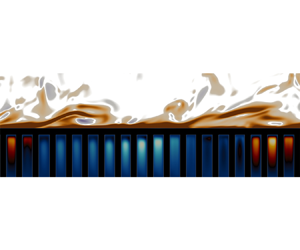
Vortex visualization using the $Q$-criterion above substrate ${\rm HP}1$ in an $x$–$y$ slice through the simulation domain. Vortex cores (light colour) are regions of $Q>0$ (high vorticity) and surrounded by a sheet (dark colour) of $Q<0$ (high shear). The hot and cold regions below the surface represent positive and negative wall-normal velocity fluctuations, respectively. Flow direction is from left to right.

Recalling the drag decomposition in figure 7, it was observed that increased streamwise-preferential anisotropy had a drag reducing effect in the ${\rm LP}$ cases, albeit a small one. As it is clear now that these cases belong to the smooth-wall-like turbulence regime, this makes the trend observed for drag change in line with the results of Gómez-de Segura & García-Mayoral (Reference Gómez-de Segura and García-Mayoral2019). In the smooth-wall-like regime, the changes in drag are due to the ‘virtual-origin’ effect (Luchini et al. Reference Luchini, Manzo and Pozzi1991; Jiménez Reference Jiménez1994; Luchini Reference Luchini1996; García-Mayoral et al. Reference García-Mayoral, Gómez-de Segura and Fairhall2019; Ibrahim et al. Reference Ibrahim, Gómez-de-Segura, Chung and García-Mayoral2021; Habibi Khorasani et al. Reference Habibi Khorasani, Lcis, Pasche, Rosti and Bagheri2022b), where the Reynolds shear stress generating quasistreamwise vortices can become displaced farther away from the surface where a slip velocity is present, resulting in a net drag reduction. This linear mechanism of passive drag reduction is only achievable so long as the flow surrounding the surface remains quasilaminar (Luchini Reference Luchini2015) and becomes negated beyond it. Owing to their smooth-wall-like quality, the drag components of ${\rm LP}1$, ${\rm LP}2$ and ${\rm LP}3$ are likely quantifiable in terms of virtual origins using the approach of Ibrahim et al. (Reference Ibrahim, Gómez-de-Segura, Chung and García-Mayoral2021), but this has not been carried out here.

5.1. Mean flow, fluctuating velocities and Reynolds shear stress

First, the mean velocity along with the fluctuations of the different velocity components are examined. Figure 16 demonstrates that the mean flow develops a region of negative shear beneath the surface. This negative shear is induced by the overlying K–H-like structures (Endrikat et al. Reference Endrikat, Modesti, García-Mayoral, Hutchins and Chung2021). As such, it is notable for the ${\rm HP}$ cases, while a very weak mean flow develops inside the substrates for the ${\rm LP}$ cases. Within the region of negative shear, the mean flow undergoes flow reversal. Larger wall-normal pore spacings cause this region to become extended and the position at which the flow undergoes reversal corresponds to the bottom of the first pore layer, i.e. $y^+\approx -{s_y}^+$. The exponential decay exhibits similarity across the different ${\rm HP}$ cases, but requires both a large enough wall-normal pore spacing and K–H-like flow to develop at the surface since the ${\rm LP}$ cases do not exhibit such a quality.

Figure 16.

Mean velocity profiles inside the substrates for the cases of table 1.

The Reynolds shear stress undergoes a sign reversal for the ${\rm HP}$ cases which the ${\rm LP}$ cases do not (figure 17). As the first pore layer becomes deeper, this reversal region becomes extended. Overall, however, $-\overline {u^{\prime }v^{\prime }}^+$ is weak below the surface. Cases ${\rm HP}2^{\prime }$ and ${\rm HP}3^{\prime }$ exhibit the same pattern as the other ${\rm HP}$ cases.

Figure 17.

Reynolds shear stress profiles inside the substrates for the cases of table 1.

For the velocity fluctuations (figure 18), all of them gradually decay towards the floor of the porous substrates where they become forcibly dampened due to the no-slip condition. However, both $u^{\prime }$ and $w^{\prime }$ undergo dampening at the bottom of each pore layer as evident by their oscillatory patterns, whereas $v^{\prime }$ largely demonstrates a monotonic decay. Considering the downward path from a surface pore-opening; the wall-normal flow entering an opening will not come across any barriers along the way towards the substrate floor since it moves through what is essentially a narrow duct. For wall-parallel flow, however, at the bottom of each pore layer the interconnected rods of the substrate's geometry will impede any in-plane motion. The overall magnitude of the spanwise velocity fluctuations is less than those of the streamwise and wall-normal velocity fluctuations, which follows from the spanwise velocity also being the least energetic velocity component at the surface of the substrates. Note that the magnitude of $v^{\prime }$ entering the substrate remains the same as it is above-surface, while the magnitudes of both $u^{\prime }$ and $w^{\prime }$ become strongly diminished. This relates to what was said earlier about $v^{\prime }$ facing less impediment as it moves through the substrate. The dense layer of solid at the substrate top strongly impedes wall-parallel motion as it penetrates into the substrate compared with wall-normal motion. Here ${\rm HP}2^{\prime }$ and ${\rm HP}3^{\prime }$ have stronger streamwise fluctuations compared with ${\rm HP}2$ and ${\rm HP}3$. This can primarily be attributed to their larger ${\mathsf{K}}_x^+$, resulting in less impedance of streamwise momentum, but may also be attributable to the stronger turbulence at the surface (figures 6 and 11), resulting in a greater modulation of the subsurface flow, an aspect which will be examined in § 6.

Figure 18.

Streamwise (a), wall-normal (b) and spanwise (c) r.m.s. velocity fluctuations within the porous substrates.

Some of the observations made here have been similarly reported for turbulent flows over engineered dense canopies (Sharma & García-Mayoral Reference Sharma and García-Mayoral2020), such as the gradual decay of the wall-normal fluctuations. Periodic dampening of the fluctuations were not reported for the canopy flows, but this is attributable to the porous substrates having layers of interconnected solid elements whereas canopy posts are isolated from one another and do not place similar restrictions on in-plane fluid motion. Similar dampening patterns were observed in the DNS of Kuwata & Suga (Reference Kuwata and Suga2017) and the experiments of Suga, Okazaki & Kuwata (Reference Suga, Okazaki and Kuwata2020).

5.2. Flow structure and features

The surface flow was described in § 4 and bearing in mind the observations made there the subsurface flow is now examined by assessing the instantaneous fluctuations within the first pore layer at $y^+\approx -15$ in figure 19. The flow fields of both ${\rm HP}2$ and ${\rm HP}3$ show spanwise elongated patterns in both their streamwise and wall-normal velocity fluctuations (figure 19a,e,b, f). The pressure fluctuations of both ${\rm HP}2$ (figure 19i) and ${\rm HP}3$ (figure 19j) reflect the patterns of their streamwise and wall-normal velocity fluctuations. Kuwata & Suga (Reference Kuwata and Suga2016) attributed the velocity fluctuations occurring within the porous substrate to the pressure fluctuations caused by the K–H-like flow at the surface. The observations made here seem to agree with this, as the turbulence in the near-surface region of both ${\rm HP}2$ and ${\rm HP}3$ falls into the K–H-like regime. The flow field of ${\rm HP}3^{\prime }$ (figure 19d,h,l) is similar to ${\rm HP}3$ (figure 19b, f,j) with no discernible differences existing between them. The flow field of ${\rm HP}2^{\prime }$ in figure 19(c,g,k) shows a stronger spanwise coherency than ${\rm HP}2$ in figure 19(a,e,i) (this greater coherency can also be observed in the flow field at $y^+=0$ in figure 32, and is attributed to the stronger K–H-like scales visible in the spectra of figure 33).

Figure 19.

Instantaneous fluctuations of (a–d) streamwise velocity, (e–h) wall-normal velocity and (i–l) pressure at $y^+\approx -15$: (a,e,i) ${\rm HP}2$; (b, f,j) ${\rm HP}3$; (c,g,k) ${\rm HP}2^{\prime }$; (d,h,l) ${\rm HP}3^{\prime }$. Flow direction is from left to right. The white regions are due to the presence of the porous substrate's rods.

More details are revealed by examining the spectra of the fluctuations within the first pore layer at $y^+=-15$, shown in figure 20. The spectra of ${\rm HP}2$ and ${\rm HP}3$ (figures 20a–d and 20e–h) show that almost no ambient turbulence scales penetrate into the substrate. Only the pore-coherent flow remains energetically discernible, as seen by its spectral signature enclosed by the green lines of figure 20. The pore-coherent flow is also diminished compared with the surface region (figure 33), but not as strongly as the ambient turbulence.

Figure 20.

Premultiplied spectral densities: (a,e,i,m) $k_x k_z E_{uu}$; (b, f,j,n) $k_x k_z E_{vv}$; (c,g,k,o) $k_x k_z E_{ww}$; (d,h,l,p) $k_x k_z E_{uv}$ at $y^+\approx -15$. Here (a–d) ${\rm HP}2$; (e–h) ${\rm HP}3$; (i–l) ${\rm HP}2^{\prime }$; (m–p) ${\rm HP}3^{\prime }$. Note the differences in the overall magnitude of the contours for the different cases. The ${\mathrm {green}}$ lines enclose the most energetically significant parts of the pore-coherent flow and the ${\mathrm {red}}$ lines those of the K–H-like rollers.

For ${\rm HP}2^{\prime }$, its stronger K–H-like scales at the surface level lead to the survival of those scales down to this depth within the substrate (the regions enclosed by the red lines in figure 20i,j,l), although they are quite weak. Despite having the same wall-normal permeability as ${\rm HP}2$, the streamwise favourable anisotropy of ${\rm HP}2'$ leads to stronger turbulent scales at the surface which are then able to penetrate deeper into the substrate.

Owing to the fact that turbulence does not survive this deep into the porous substrates for ${\rm HP}2$, ${\rm HP}3$, ${\rm HP}2'$ and ${\rm HP}3'$, the coherent patterns observed in their flow fields (figure 19) must be attributed to the pore-coherent flow which remains detectable at this depth. The broadband spanwise intensification of the pore-coherent flow, however, is imparted to it from the surface level turbulence which possess spanwise coherent energetic scales. The modulation persists throughout the substrate and hence why the spectra in figure 20 show long patches of spanwise energetic scales, particularly for the wall-normal velocity.

Ultimately, for the porous substrates under consideration here, there exists a notable pore-coherent flow component below the surface, and in some cases weak scales of ambient turbulence related to the K–H-like instability. Similarly, in flows over canopies the fluctuations below the canopy tip-plane are attributed to the strong overlying cross-flow rollers that develop due to the existence of a perturbed mixing layer (Sharma & García-Mayoral Reference Sharma and García-Mayoral2020). As mentioned previously in § 3.5, for a mixing layer to emerge over porous media, very high effective surface permeability (or permeability Reynolds number) is required (Jiménez et al. Reference Jiménez, Uhlmann, Pinelli and Kawahara2001; Manes et al. Reference Manes, Poggi and Ridolfi2011). Outside of this mixing layer regime, the notable flow activity below the surface mainly resides in the pore-coherent scales of the flow which undergo modulation by the turbulence at substrate's surface. Manes et al. (Reference Manes, Poggi and Ridolfi2011) examined whether the resulting eddy structures over their porous foams shared the same characteristics as those reported over canopies and which are associated with an inflectional instability of the mean velocity (White & Nepf Reference White and Nepf2007). They observed this to not be the case for low to intermediate ranges of permeability. This also applies to the porous substrates examined in this paper and the analysis done to quantify this is gathered in Appendix B.

Before proceeding further, as a final examination to see whether the flow structure inside the substrates undergoes any notable change deeper inside the substrate, the instantaneous fluctuations as well as the spectra at $y^+\approx -55$ for case ${\rm HP}1$ alone are shown in figure 21. One can witness that the patterns are overall similar to those observed at $y^+\approx -15$ for the rest of the ${\rm HP}$ cases, with the most notable scales of motion again being those of the pore-coherent flow, while a weak footprint of the K–H-like scales are also present. The existence of the latter at this depth is of course attributable to the stronger overlying K–H-like structures of ${\rm HP}1$. In addition, ${\rm HP}1$ also lacks interconnected rod layers inside the substrate which would impede downward directed flow. The explanation for the spanwise coherence of the flow field is similar to what was previously described for the flow at the shallower depth of $y^+\approx -15$. The spectral signature of the pore-coherent flow which encompasses a range of streamwise scales is repeated along the spanwise direction at intervals equal to the spanwise spacing (${\lambda _z}^+={s_z}^+$), i.e. between two consecutive pores along this direction. In essence, the patches are collections of narrow fingers of streamwise velocity which are confined to the pores due to a microchannelization effect. These flow elements appear as a spanwise coherent region macroscopically due to being modulated in amplitude, which is what will be examined next.

Figure 21.

Instantaneous velocity fluctuations and premultiplied spectral energy densities of case ${\rm HP}1$ at $y^+\approx -55$: (a) streamwise fluctuations, (b) wall-normal fluctuations, (c) pressure fluctuations; (d) $k_x k_z E_{uu}$, (e) $k_x k_z E_{vv}$, ( f) $k_x k_z E_{ww}$ and (g) $k_x k_z E_{uv}$. The ${\mathrm {green}}$ lines enclose the most energetically significant parts of the pore-coherent flow and the ${\mathrm {red}}$ lines the surviving turbulence belonging to the K–H-like scales.