1 Introduction
An improved understanding of the physical mechanisms governing supersonic jet-impingement flows and their associated noise generation mechanisms is of great practical relevance for aeronautical and astronautical applications. A few example applications where jet-impingement noise is relevant are jet impingement during rocket launch, initial stage of launch abort, multi-stage rocket separation, jet-engine exhaust impingement for short take-off and landing (STOL) and powered vertical take-off and landing (VTOL) aircraft. The noise generation during rocket launch is a major safety concern because high-amplitude pressure oscillations may lead to sonic fatigue failure of nearby sensitive structural or electronic components (Clarkson Reference Clarkson1994). These types of flow problems are very complex and involve a variety of interconnected flow physics. Despite the wide relevance of these types of flows, there are few research studies investigating the flow physics and the noise generation process for non-vertical jet impingement. This paper is concerned with the noise generation mechanisms for a supersonic Mach number
 $M=1.8$
perfectly expanded jet impinging on a
 $45^{\circ }$
inclined plate. The noise source identification and characterization methods employed for the jet-impingement problem are based on methods that were mainly developed for free jets. To understand noise generation for jet impingement, it is beneficial to revisit some of the methods and findings for noise generation in free jets.
1.1 Identification of noise sources and noise generation mechanisms for free jets
In contrast to non-vertical jet-impingement flows, the physical mechanisms for acoustic sound generation in subsonic and supersonic free jets have been analysed in great detail by a large number of researchers, including Tam & Chen (Reference Tam and Chen1994), Tam (Reference Tam1995), Tam, Golebiowski & Seiner (Reference Tam, Golebiowski and Seiner1996), Freund (Reference Freund2001), Panda & Seasholtz (Reference Panda and Seasholtz2002), Bogey, Bailly & Juvé (Reference Bogey, Bailly and Juvé2003), Panda, Seasholtz & Elam (Reference Panda, Seasholtz and Elam2005), Bogey & Bailly (Reference Bogey and Bailly2007) and Tam et al. (Reference Tam, Viswanathan, Ahuja and Panda2008), among many others. An early fundamental finding – turbulent jet flows contain both fine- and large-scale turbulent structures – is now generally accepted and has great importance for understanding noise generation in free jets. Crow & Champagne (Reference Crow and Champagne1971) and Brown & Roshko (Reference Brown and Roshko1974) were among the first researchers to report the occurrence of large coherent flow structures in turbulent flows, in contrast to the previous belief that these flows consist only of multiple distributed small eddies. The large coherent flow structures emerging in turbulent jet flows are regarded as a manifestation of Kelvin–Helmholtz type instabilities of the turbulent shear layer which saturate at nonlinear amplitudes (Michalke Reference Michalke1984). The instability-wave-based models for sound generation by Morris & Tam (Reference Morris and Tam1979) and Tam & Burton (Reference Tam and Burton1984) came about by the aforementioned finding. For the current jet-impingement problem, these large coherent flow structures are expected to also play an important role in the noise generation process. Tam & Chen (Reference Tam and Chen1994) and Tam (Reference Tam1995) proposed a two-noise source model which is explicitly based on the realization that fine-grained turbulence and large coherent structures are generating distinct noise signatures. The two universal spectra put forward by Tam et al. (Reference Tam, Golebiowski and Seiner1996) were able to fit all jet-noise data in their database. Tam et al. (Reference Tam, Viswanathan, Ahuja and Panda2008) refer to the noise spectrum predominantly generated by large-scale coherent flow structures as the ‘F-spectrum’ or ‘peaky spectrum’. The noise spectrum that fits the data in the upstream and sideline directions is referred to as the ‘G-spectrum’ or ‘broad spectrum’ and is dominated by noise generation from small-scale turbulence. A superposition considering both spectra is used to fit the data in the intermediate regions. Various research studies by Tam (Reference Tam1998), Dahl & Papamoschou (Reference Dahl and Papamoschou2000), Viswanathan (Reference Viswanathan2002), Viswanathan (Reference Viswanathan2004) and Tam et al. (Reference Tam, Viswanathan, Ahuja and Panda2008) provide convincing evidence of the validity of these two acoustic similarity spectra for free jets.
The noise generation mechanisms associated with these large-scale coherent flow structures can be (and have been) studied by utilizing the causality method. Appendix B provides the theoretical background on the causality method as it was employed in this research. The causality method involves the computation of cross-correlations between flow quantities inside the source region and the acoustic pressure in the far field. It is the most direct way of identifying noise sources (Tam et al.
Reference Tam, Viswanathan, Ahuja and Panda2008). In some of the first applications of this method, Rackl (Reference Rackl1973) and Hurdle, Meecham & Hodder (Reference Hurdle, Meecham and Hodder1974) used the incompressible pressure inside the jet to study the relevant flow physics. More recently, Panda & Seasholtz (Reference Panda and Seasholtz2002) employed a Rayleigh-scattering-based technique to obtain density fluctuations in the plume of a fully expanded unheated free jet. These density fluctuations were cross-correlated with acoustic pressure measurements in the far field to investigate the noise generation process. Strong correlations from the centreline of the jet were obtained in a region downstream of the potential core, extending over many diameters for Mach numbers
 $0.6\leqslant M\leqslant 1.8$
. In Panda et al. (Reference Panda, Seasholtz and Elam2005), this work was extended by cross-correlating the acoustic pressure in the far field with additional flow quantities, such as the density
 ${\it\rho}$
, axial velocity
 $u$
, radial velocity
 $v$
and momentum fluxes
 ${\it\rho}uu$
and
 ${\it\rho}vv$
, inside the jet plume. The strongest cross-correlation, here denoted by
 $\langle \ast ;\ast \rangle$
, occurred for
 $\langle {\it\rho}uu;p^{\prime }\rangle$
, where the cross-correlations for the first-order terms,
 $\langle {\it\rho}^{\prime }\overline{u}\overline{u};p^{\prime }\rangle$
and
 $\langle \overline{{\it\rho}}\overline{u}u^{\prime };p^{\prime }\rangle$
, and third-order term,
 $\langle {\it\rho}^{\prime }u^{\prime }u^{\prime };p^{\prime }\rangle$
, were higher than the cross-correlations for the second-order terms,
 $\langle \overline{{\it\rho}}u^{\prime }u^{\prime };p^{\prime }\rangle$
and
 $\langle {\it\rho}^{\prime }\overline{u}u^{\prime };p^{\prime }\rangle$
. The correlations for
 $\langle v^{\prime };p^{\prime }\rangle$
and
 $\langle {\it\rho}vv;p^{\prime }\rangle$
were weaker in the downstream direction and not measurable in the sideline direction. All of the above findings are based on the normalized cross-correlation function. In this paper, we employ both normalized and non-normalized cross-correlation functions because the findings provided by these functions complement one another by highlighting different aspects of the noise generation process. The analysis of the results in Panda et al. (Reference Panda, Seasholtz and Elam2005) demonstrated that the measured correlations are strong for fluctuations from large coherent flow structures, whereas the correlations from small-scale structures are below the noise floor.
Michalke (see Michalke Reference Michalke1984, Reference Michalke1983, Reference Michalke1977) demonstrated, by analysing the noise generation of a round jet decomposed into azimuthal modes with axial and radial coherence, that low-order azimuthal modes are significant noise contributors. For a non-compact noise source, a significant amount of the noise at the receiver microphone originates from an extended coherent volume. The weak correlations for the compact noise sources composed of fine-scale turbulence are expected considering that the receiver microphone obtains noise from a large number of compact sources in the jet. Since the noise source is small and localized, the correlation of acoustic pressure with a small region of turbulent fluctuations is statistically insignificant (Tam et al. Reference Tam, Viswanathan, Ahuja and Panda2008). Although small eddies are inefficient radiators (Panda et al. Reference Panda, Seasholtz and Elam2005), the accumulated sound from a large number of small eddies in the large volume of turbulent shear flow is significant. In this paper, we focus on noise generation from non-compact sources similar to the work by Panda et al. (Reference Panda, Seasholtz and Elam2005), considering that the correlations from small-scale turbulent structures are weak. This approach is justified since it can be assumed that the predominant noise generation mechanisms for the current jet-impingement problem are associated with non-compact noise sources (according to Tsutsumi et al. (Reference Tsutsumi, Takaki, Nakanishi, Okamoto and Teramoto2014), Akamine et al. (Reference Akamine, Nakanishi, Okamoto, Teramoto, Okunuki and Tsutsumi2014) and Nakanishi et al. (Reference Nakanishi, Okamoto, Teramoto, Okunuki and Tsutsumi2012)).
Another important study was conducted by Freund (Reference Freund2001), who solved Lighthill’s equation numerically and verified the procedure by comparison with direct numerical simulation (DNS). The source terms based on Lighthill’s theory were obtained by utilizing direct numerical simulation results of a cold Mach 0.9, Reynolds number 3600 turbulent jet. Prior to applying the volume integration, the source terms were Fourier transformed in the axial coordinate direction and time, and then filtered to separate out the radiating part of the solution. Space–time correlations demonstrated that the sources predominantly emitting noise in the downstream direction are non-compact, and the fraction of the source emitting noise at angles larger than
 $45^{\circ }$
is (spatially) stationary. This study affirms that by correctly accounting for the radiating part in the source terms of Lighthill’s equation, the far-field noise signature can be predicted by Lighthill’s theory. Thus, the causality method based on Lighthill’s theory and accounting for the radiating part of the solution, as employed in this paper, can be used to identify and characterize the noise sources. In another application of the causality method, Bogey & Bailly (Reference Bogey and Bailly2007) employed large-eddy simulations (LES) of subsonic (
 $M=0.6$
and
 $M=0.9$
) isothermal jets for two Reynolds numbers
 $Re_{D}=1700$
and
 $Re_{D}\geqslant 10^{5}$
to analyse cross-correlations between fluctuating quantities in the turbulent flow and the sound pressure field. Bogey & Bailly (Reference Bogey and Bailly2007) carried out a detailed analysis to further the understanding of how the coherent flow structures generate noise. The analysis suggests that the noise source, which dominates in the downstream direction, is located on the centreline of the jet at the end of the potential core, which is supported by findings of Panda et al. (Reference Panda, Seasholtz and Elam2005). This area of the jet extends over a large axial distance with a dominant Strouhal number and is characterized by strong levels of intermittency and high convection velocities. It was conjectured that the directional jet-noise source, which is dominant in the downstream direction, is associated with the periodic and intermittent intrusion of vortical structures into the jet core, as described in Bogey et al. (Reference Bogey, Bailly and Juvé2003).
1.2 Vertical jet impingement
The flow physics for vertical jet impingement has been studied by many researchers in the past (Ginzburg, Semiletenko & Uskov Reference Ginzburg, Semiletenko and Uskov1970; Nakatogawa, Hirata & Kukita Reference Nakatogawa, Hirata and Kukita1971; Ho & Nosseir Reference Ho and Nosseir1981; Powell Reference Powell1988; Henderson & Powell Reference Henderson and Powell1993; Krothapalli et al. Reference Krothapalli, Rajkuperan, Alvi and Lourenco1999; Henderson Reference Henderson2002; Henderson, Bridges & Wernet Reference Henderson, Bridges and Wernet2005; Dauptain, Gicquel & Moreau Reference Dauptain, Gicquel and Moreau2012). When a jet impinges on a surface, high-pressure amplitude fluctuations are generated on the solid surface. For certain nozzle pressure ratios and plate-to-nozzle distances, discrete acoustic tones may occur in the far-field acoustic spectra. This tonal noise can be explained by a feedback loop between the large-scale coherent flow structures convected downstream and the pressure waves propagating upstream producing resonance frequencies. The acoustic far field generated by a launching rocket does not, however, commonly contain signs of tonal noise but rather broadband noise characteristics that appear to be associated with various interactions of large-scale turbulent structures (Eldred Reference Eldred1971; Varnier Reference Varnier2001). Furthermore, prior numerical simulations by Brehm et al. (Reference Brehm, Sozer, Moini-Yekta, Housman, Barad, Kiris, Vu and Parlier2013) and Tsutsumi et al. (Reference Tsutsumi, Takaki, Nakanishi, Okamoto and Teramoto2014) and the experimental results of Nakanishi et al. (Reference Nakanishi, Okamoto, Teramoto, Okunuki and Tsutsumi2012) and Akamine et al. (Reference Akamine, Nakanishi, Okamoto, Teramoto, Okunuki and Tsutsumi2014) did not exhibit a feedback phenomenon for the current configuration.
1.3 Jet impingement on an inclined plate
Non-vertical jet impingement of a supersonic ideally expanded cold jet with different nozzle-to-plate distances and different impingement angles has been previously studied both numerically (see Nonomura & Fujii Reference Nonomura and Fujii2010, Reference Nonomura and Fujii2011; Nonomura, Goto & Fujii Reference Nonomura, Goto and Fujii2011; Tsutsumi et al.
Reference Tsutsumi, Nonomura, Fujii, Nakanishi, Teramoto and Okamoto2012, Reference Tsutsumi, Takaki, Nakanishi, Okamoto and Teramoto2014; Brehm et al.
Reference Brehm, Sozer, Moini-Yekta, Housman, Barad, Kiris, Vu and Parlier2013) and experimentally (see Nakanishi et al.
Reference Nakanishi, Okamoto, Teramoto, Okunuki and Tsutsumi2012; Akamine et al.
Reference Akamine, Nakanishi, Okamoto, Teramoto, Okunuki and Tsutsumi2014). The flow conditions employed in this paper are identical or very similar to the flow conditions used in the numerical simulations or experiments discussed in this section. Solving the three-dimensional Navier–Stokes equations with a modified weighted compact nonlinear scheme, Nonomura et al. (Reference Nonomura, Goto and Fujii2011) studied the effects of nozzle-to-plate distance and jet temperature on the acoustic field of ideally expanded supersonic jets impinging on a
 $45^{\circ }$
inclined plate. Analysing distributions of the overall sound pressure level (OASPL) and octave-banded sound pressure level (SPL) in the symmetry plane, Nonomura et al. (Reference Nonomura, Goto and Fujii2011) observed at least three types of possible noise sources: (i) Mach wave radiation associated with supersonically convected large-scale turbulent flow structures (similar to free jets), (ii) acoustic waves generated in the impingement region and (iii) Mach waves generated in the shear layer of the supersonic wall jet downstream of the impingement region. They also emphasized that study of the second mechanism of noise generation is important since frequently employed empirical methods (in Eldred (Reference Eldred1971) and Haynes & Kenny (Reference Haynes and Kenny2009)) for the estimation of rocket-plume acoustics do not account for these waves. Nonomura & Fujii (Reference Nonomura and Fujii2011) simulated a supersonic Mach
 $2$
ideally expanded jet with a Reynolds number of
 $Re=25\,000$
impinging on an inclined plate with an impingement angle of
 $45^{\circ }$
and a plate-to-nozzle distance of
 $5D$
. Two computational grids with vastly different grid sizes were used to study the effects from near-wall turbulent structures on the aeroacoustic noise field. The larger computational grid was carefully designed to resolve the turbulent boundary layer. By comparing the acoustic data in the far field, it was concluded that the essential flow features responsible for noise generation appear to be insensitive to the resolution of the turbulent boundary layer. This information proved useful for the present simulation set-up.
Honda et al. (Reference Honda, Nonomura, Fujii and Yamamoto2011) studied the effect of the plate angle on the aeroacoustic wave-propagation pattern for three different impingement angles
 $30^{\circ }$
,
 $45^{\circ }$
and
 $60^{\circ }$
using a higher-order modified weighted compact nonlinear scheme at
 $Re=100\,000$
. For all three impingement angles, they found that the same three acoustic noise sources observed by Nonomura et al. (Reference Nonomura, Goto and Fujii2011) are present. Shock-induced separation was observed on the impingement plate for all impingement angles. It was conjectured to play an important role in the noise generation process from the wall jet region. The impingement angle affects the predominant wave-propagation direction and the magnitudes of sound pressure levels in the far field. Akamine et al. (Reference Akamine, Nakanishi, Okamoto, Teramoto, Okunuki and Tsutsumi2014) obtained microphone measurements in the far field, Schlieren visualization and static wall pressure measurements for an ideally expanded Mach 1.8 jet impinging on a
 $45^{\circ }$
inclined plate. The conditions are identical to the ones used in this work with
 $Re=1.6\times 10^{6}$
. Two main propagation directions were identified, at
 $75^{\circ }$
and
 $120^{\circ }$
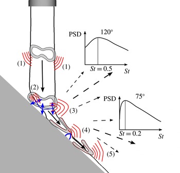
relative to the jet axis, in agreement with previous experimental findings by Nakanishi et al. (Reference Nakanishi, Okamoto, Teramoto, Okunuki and Tsutsumi2012). The far-field acoustic spectrum of an observer point in the
 $75^{\circ }$
direction to the jet axis exhibits a broadband peak at a Strouhal number of approximately
 $St=fD/u_{j}\approx 0.2$
where
 $f$
is frequency,
 $D$
is nozzle exit diameter and
 $u_{j}$
the mean velocity at the nozzle exit. The far-field acoustic spectrum of an observer point in the
 $120^{\circ }$
direction has a wider broadband peak at approximately
 $St\approx 0.5$
. Tsutsumi et al. (Reference Tsutsumi, Takaki, Nakanishi, Okamoto and Teramoto2014) conducted numerical simulations for the same flow conditions (
 $Re=1.6\times 10^{6}$
) employing a zonal hybrid LES/Reynolds-averaged Navier–Stokes (RANS) methodology with a sixth-order accurate compact scheme and a tenth-order accurate low-pass filter. They were able to predict the main features of the overall SPL in the far field (within
 $\pm$
5 dB) and the power spectral density (PSD) spectrum at each of the six microphone locations recorded in experiments. By employing conditional sampling, they were able to visualize that the peak at
 $120^{\circ }$
is related to acoustic waves originating in the impingement region around the plate shock. Similarly, the pressure waves originating at the first tail shock appear to predominantly propagate in the
 $75^{\circ }$
direction.
Although the most dominant noise source regions have been identified in previous experimental and computational studies, the detailed mechanisms of noise generation are not well understood at this point. Hence, this work aims at providing a deeper physical understanding of the relevant noise generation mechanisms. The present paper is organized as follows. The numerical methods, computational set-up and a discussion of the simulation strategy are provided in § 2. The analysis of the turbulent flow field in § 3 is divided into two parts, namely the turbulent jet upstream of the impingement point and the deflected turbulent wall jet flow downstream of the impingement point. The coherence in the source region is analysed by employing proper orthogonal decomposition (POD). The acoustic near-field and far-field wave-propagation patterns are investigated in § 4. The computational results in §§ 3 and 4 are compared with a limited set of available experimental data by Akamine et al. (Reference Akamine, Nakanishi, Okamoto, Teramoto, Okunuki and Tsutsumi2014). In § 5, the causality method is used to further the understanding of the noise generation process for jet-impingement flows. The main objective in § 5 is to link the flow characteristics of the source region discussed in § 3 to the emitted acoustic pressure field discussed in § 4. Section 6 provides a detailed discussion on the identified noise sources and the noise generation mechanisms.
2 Computational methods
2.1 Numerical methods
For the current simulation of the jet-impingement problem, the unsteady compressible Navier–Stokes equations are solved in a conservative finite-difference formulation on block-structured Cartesian grids employing a sharp immersed boundary method (see Mittal et al. Reference Mittal, Dong, Bozkurttas, Najjar, Vargas and von Loebbecke2008; Brehm & Fasel Reference Brehm and Fasel2013; Brehm, Hader & Fasel Reference Brehm, Hader and Fasel2015b ) and an adaptive mesh refinement (AMR) scheme utilizing an entropy adjoint approach following Fidkowski & Roe (Reference Fidkowski and Roe2010). The solver is designed to dynamically track important flow features as they develop over time by utilizing the AMR solution procedure. To account for flow discontinuities, a sixth-order accurate shock-capturing weighted essentially non-oscillatory (WENO) scheme is utilized. The characteristic variable transformation is applied to a Rusanov-type flux vector splitting scheme. The accuracy and computational efficiency of the higher-order shock-capturing schemes of the current solver have been previously analysed in Brehm et al. (Reference Brehm, Barad, Housman and Kiris2015a ). The viscous terms are discretized with fourth-order accuracy. The fourth-order accurate explicit Runge–Kutta scheme is used for time integration. Additional information about the numerical schemes and their properties can be found in Kiris et al. (Reference Kiris, Barad, Housman, Sozer, Brehm and Moini-Yekta2014).
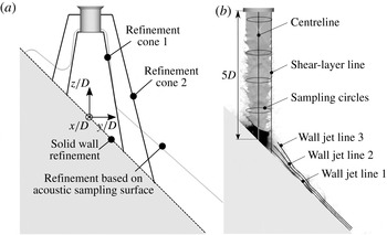
(a) Mesh refinement regions in the computational domain. (b) Sampling lines used for postprocessing of the unsteady flow field, with greyscale contours of temperature.

2.2 Computational set-up
The mesh topology for the current simulation is schematically illustrated in figure 1(a). Grid refinement was applied in the turbulent jet, the impingement region and the wall jet where high unsteadiness and large gradients were expected. Different volume tagging surfaces were used to control the grid spacing in the impingement region (figure 1
a). Two cone sections (refinement cones 1 and 2) were used to control the volume mesh spacing in the turbulent jet, and the acoustic sampling surface used in § 4 was employed for volume tagging of the wall jet, as illustrated in figure 1(b). Within the turbulent jet, we used a grid spacing that corresponded to
 $D/{\rm\Delta}x=200$
grid points across the nozzle diameter. The mesh was subsequently coarsened by a factor of 2 in the second cone and in the wall jet. Overall, a total of approximately
 $0.6$
billion grid points were used in the current mesh. A grid refinement study was previously conducted in Brehm et al. (Reference Brehm, Sozer, Moini-Yekta, Housman, Barad, Kiris, Vu and Parlier2013) and Housman, Brehm & Kiris (Reference Housman, Brehm and Kiris2013). For the current simulation, the origin of the coordinate system is located at the intersection point of the nozzle centre axis with the impingement plate, where the
 $z$
-axis points towards the nozzle. The nozzle exit is located five nozzle exit diameters (
 $z=5D$
) above the origin (figure 1
b). Figure 1(b) also shows different sampling lines and sampling circles that are used throughout the paper for probing the unsteady flow field. The computational domain extends
 $50D$
in each coordinate direction, and characteristic boundary conditions are used to avoid wave reflections from the domain boundaries. Further, the computational mesh coarsens towards the domain boundaries, providing additional numerical dissipation to eliminate spurious reflections. The nozzle ejects an approximately ideally expanded jet which impinges on the
 $45^{\circ }$
inclined plate. The impingement angle is defined as the angle between the y-axis and the normal vector of the impingement plane, thus vertical impingement is obtained for
 $90^{\circ }$
.
The flow conditions are based on two experiments carried out by Nakanishi et al. (Reference Nakanishi, Okamoto, Teramoto, Okunuki and Tsutsumi2012) and Akamine et al. (Reference Akamine, Nakanishi, Okamoto, Teramoto, Okunuki and Tsutsumi2014) at the UT-Kashiwa hypersonic and high-temperature wind tunnel (Kashiwa wind tunnel). The experimental investigations have been accompanied by several numerical studies (see Nonomura & Fujii Reference Nonomura and Fujii2010; Nonomura et al.
Reference Nonomura, Goto and Fujii2011; Nakanishi et al.
Reference Nakanishi, Okamoto, Teramoto, Okunuki and Tsutsumi2012; Tsutsumi et al.
Reference Tsutsumi, Nonomura, Fujii, Nakanishi, Teramoto and Okamoto2012, Reference Tsutsumi, Takaki, Nakanishi, Okamoto and Teramoto2014). The jet in this experiment was cold with
 $T=300$
K to exclude any high-temperature effects. The supersonic perfectly expanded jet reached a Mach number of
 $M=1.8$
at the nozzle exit. In an RANS precursor calculation, the nozzle flow was solved separately to provide boundary conditions for the LES. The boundary layer and momentum thicknesses at the nozzle exit were roughly
 $5.5\times 10^{-2}D$
and
 $8.7\times 10^{-3}D$
. For the high-fidelity simulation, the exterior of the nozzle was modelled in accordance with the experimental set-up. The simulations were performed by assuming an ideal gas with a specific heat ratio of
 ${\it\gamma}=1.4$
and a constant specific heat capacity of
 $c_{p}=1005~\text{J}~\text{kg}^{-1}~\text{K}^{-1}$
. The molecular viscosity was calculated using Sutherland’s law assuming air. For the current simulations, the flow conditions at the actual nozzle exit were
 $M=1.8045$
,
 $V_{e}=488.14~\text{m}~\text{s}^{-1}$
and
 $p_{e}=100\,794$
Pa. The differences from a theoretical perfectly expanded Mach
 $1.8$
jet were
 ${\rm\Delta}M/M\approx 0.25\,\%$
,
 ${\rm\Delta}V_{e}/V_{e}\approx 0.52\,\%$
and
 ${\rm\Delta}p_{e}/p_{e}\approx 0.24\,\%$
. Close to a billion grid points were used to simulate the jet flow with a Reynolds number of
 $Re=V_{e}D/{\it\nu}=1.6\times 10^{6}$
, where
 $V_{e}$
is the nozzle exit velocity,
 $D$
is the nozzle exit diameter and
 ${\it\nu}$
is the kinematic viscosity of air at the nozzle exit temperature. The physical time step was
 ${\rm\Delta}tV_{e}/D=2\times 10^{-3}$
and the simulation ran for about
 $250\,000$
time steps (
 $TV_{e}/D=500$
). Only the last
 $100\,000$
time steps (
 $TV_{e}/D=200$
) were used for postprocessing. For the POD analysis, only about half of the postprocessing time interval was used due to large memory requirements. The POD results for three windows with
 $50\,\%$
overlap showed close agreement. The analysis in this paper is mainly focused on two-dimensional cut-planes, while the noise sources are truly three-dimensional. The analysis based on two-dimensional cut-planes provides, however, a good idea about the essential features of the noise generation mechanisms. A three-dimensional analysis may provide additional insight about the acoustic noise generation mechanisms. Throughout the paper, all flow quantities (if not otherwise stated) are normalized with exit flow conditions, where the reference length scale
 $L_{ref}$
, pressure
 $p_{ref}$
and velocity
 $V_{ref}$
are
 $D$
,
 $p_{e}$
and
 $V_{e}$
respectively. The velocity components of
 $\boldsymbol{v}_{cart}=[u,v,w]$
refer to the components in the Cartesian reference frame. In some parts a cylindrical coordinate system is utilized with the velocity vector in the form
 $\boldsymbol{v}_{cyl}=[v_{r},v_{{\it\Theta}},w]$
, where
 $v_{r}$
and
 $v_{{\it\Theta}}$
refer to the radial and azimuthal velocity components.
2.3 Computational simulation strategy
It is well known that DNS is currently limited to Reynolds number regimes of up to
 $O(10^{4})$
due to cost constraints. Hence, DNS is not feasible for the current flow conditions and we will rely on large-eddy simulation (LES) in which molecular viscosity has little effect on the large-scale flow structures (probably less effect than the inflow shear-layer thickness or state, laminar versus turbulent, as suggested by Shur, Spalart & Strelets (Reference Shur, Spalart and Strelets2005b
)). The current computational simulation strategy with respect to nozzle inflow conditions and the subgrid-scale modelling is closely aligned with the recommendations of Shur, Spalart & Strelets (Reference Shur, Spalart and Strelets2005a
) and Shur et al. (Reference Shur, Spalart and Strelets2005b
), who discuss strategies for turbulent jet flow simulations. They demonstrated that their simulation approach to predict the noise field is very accurate and computationally efficient.
For the current simulations, we are employing an implicit large-eddy simulation (ILES) approach. In contrast to classical LES, which employs an explicitly computed subgrid scale (SGS) closure, ILES relies on the inherent regularization mechanism through the truncation error of the convective fluxes, which is also referred to as the implicit SGS model (Hu & Adams Reference Hu and Adams2011) or numerical LES (Pope Reference Pope2004). The primary role of the SGS model is to remove the energy that would cascade down to the unresolved scales. Hence, the numerical scheme must be chosen carefully to provide a physically consistent implicit SGS model. In the current study, the modified sixth-order accurate WENO scheme (Hu, Wang & Adams Reference Hu, Wang and Adams2010) was used due to its superior physically motivated scale separation properties. Hu & Adams (Reference Hu and Adams2011) have demonstrated that the modified sixth-order accurate WENO scheme reproduces the Kolmogorov range of the turbulent kinetic-energy spectrum at the limit of infinite Reynolds number independent of grid resolution, while maintaining the shock-capturing capabilities of the original WENO-CU6. A detailed discussion and comparison of higher-order shock-capturing schemes within the current solver for various test problems containing turbulent flows and shocks is provided in Brehm et al. (Reference Brehm, Barad, Housman and Kiris2015a ). It is important to point out that our experience, as well as the results from other research studies (see Shur et al. Reference Shur, Spalart and Strelets2005a ,Reference Shur, Spalart and Strelets b ; Brehm et al. Reference Brehm, Sozer, Moini-Yekta, Housman, Barad, Kiris, Vu and Parlier2013), confirms that for simulations of turbulent flows away from solid boundaries, the ILES approach is a well-suited simulation strategy. Moreover, the ILES approach is very efficient in utilizing the available grid resolution for capturing the shear-layer transition process and modelling salient features of the turbulent flow. Preliminary studies and other researchers (Shur et al. Reference Shur, Spalart, Strelets and Travin2003, Reference Shur, Spalart and Strelets2005b ) have even demonstrated that the transition of the shear layer can be delayed and the proper amount of turbulence generation is not generated as well when utilizing a suboptimal explicit SGS model for these flow conditions. In addition, as pointed out in § 1.3, Nonomura & Fujii (Reference Nonomura and Fujii2011) confirmed for very similar flow conditions that the near-wall turbulent structures within the wall jet boundary layer play an insignificant role in the noise generation process.
Another important detail for the computational set-up is the specification of the nozzle exit boundary conditions. As pointed out in Zaman (Reference Zaman2012), the internal nozzle geometry plays a critical role in determining the nozzle exit boundary layer state. Recent studies for free jets (Bogey & Bailly Reference Bogey and Bailly2003; Lew et al. Reference Lew, Uzun, Blaisdell and Lyrintzis2004; Zaman Reference Zaman2012; Brès et al. Reference Brès, Jaunet, Le Rallic, Jordan, Colonius and Lele2015, and others) have shown that the far-field acoustic spectra are affected by the details of the nozzle exit boundary layer flow, such as boundary layer thickness and turbulent intensity. Zaman (Reference Zaman2012) showed for subsonic jet flows how the nozzle exit boundary layer state affects the emitted noise signature. He found that a noisier nozzle involved a highly disturbed laminar (or nominally laminar) boundary layer in contrast to the turbulent exit boundary layer of a more silent nozzle. Ideally, the nozzle exit flow would be modelled appropriately as a nominally laminar or turbulent boundary layer convecting unsteadiness into the jet shear layer. In the experimental set-up, however, the nozzle exit boundary layer state was not determined, making it difficult to provide the correct level of turbulence intensity. Since the available computational resources are not adequate for simulating the entire interior nozzle flow, we are relying on the fact that the shear layer will essentially transition and create a more energetic unsteadiness (ultimately a turbulent flow state) than in the nozzle boundary layer flow. For free jet flow simulations, some researchers (for example Freund Reference Freund2001; Bogey & Bailly Reference Bogey and Bailly2007) have applied unsteady forcing to seed unsteadiness in the transitional shear layer. One natural choice would be to introduce perturbations based on linear stability theory (LST), as discussed in Michalke (Reference Michalke1984), i.e. Tollmien–Schlichting waves in boundary layers and Kelvin–Helmholtz waves in shear layers. Bogey & Bailly (Reference Bogey and Bailly2007) followed a different strategy and excited the mean flow with randomized perturbations in the form of induced velocities from a vortex ring (see also Bogey et al. Reference Bogey, Bailly and Juvé2003). This was done very carefully to ensure a proper breakup of the potential core within a reasonable distance. It is cumbersome to achieve a realistic scenario with respect to frequencies and amplitudes not knowing the actual conditions in the experiment. Previous studies for jet-impingement flows, however, have demonstrated that the dominant noise sources are located in the vicinity of the impingement plate. These noise sources appear to be far less sensitive to the details of the nozzle exit boundary layer.
Hence, in the current simulation, we did not use any type of forcing based on linear stability theory and/or random noise, which on the other hand prevents accidental introduction of parasitic noise (Shur et al.
Reference Shur, Spalart and Strelets2005b
). For the jet-impingement problem, an elevated acoustic background noise level was continuously generated by the impinging jet, seeding unsteadiness in the shear layer. No numerical artefacts such as a preferred frequency response that could cause some type of artificial feedback were observed in the simulations. The grid convergence study previously presented in Brehm et al. (Reference Brehm, Sozer, Moini-Yekta, Housman, Barad, Kiris, Vu and Parlier2013) and Housman et al. (Reference Housman, Brehm and Kiris2013) ensured that the relevant flow features captured with the ILES approach were sufficiently grid converged and did not contain a spurious numerical feedback mechanism. Moreover, comparison of the current grid resolution with computational set-ups of similar research studies suggested that the current grid resolution was sufficient to study the relevant flow physics associated with noise generation. For example, at similar flow conditions (
 $Re_{D}=1\times 10^{6}$
) the spatial resolution in Dauptain et al. (Reference Dauptain, Gicquel and Moreau2012) was coarser than the final mesh used here, despite the fact that the temporal and spatial resolution accuracy of the current simulation was higher. Dauptain et al. (Reference Dauptain, Gicquel and Moreau2012) obtained excellent agreement in a detailed comparison with experimental data reported by Henderson et al. (Reference Henderson, Bridges and Wernet2005). Their finest grid spacing at the nozzle lip corresponded to roughly
 $60$
points per nozzle diameter. The azimuthal resolution along the circumference of the nozzle was approximately
 $160$
points. Dauptain et al. (Reference Dauptain, Gicquel and Moreau2012) used a third-order Taylor–Galerkin method (Donea Reference Donea1984) in space with hyperviscosity at shocks on an unstructured mesh. Within the turbulent jet, our temporally fourth-order accurate and spatially sixth-order accurate solver utilized
 $200$
grid points per diameter in all directions on a Cartesian grid, which corresponds to
 $290$
to
 $500$
grid points along the circumference of the nozzle. (On a Cartesian grid, it is not clear how the circumferential grid spacing should be defined. The lower grid point estimate takes the diagonal spacing (
 $\sqrt{3}{\rm\Delta}x$
) within a cubic cell and the larger grid point estimate uses the actual edge length (
 ${\rm\Delta}x$
) of the cell.)
3 Characterization of jet-impingement flow features
The first part of this paper focuses on characterizing the flow features within the source region, which we also refer to as the LES region. Shortly after leaving the nozzle exit, the jet goes through a complicated transition process that is initiated in the shear layer. The turbulent shear layer subsequently thickens towards the downstream direction to encompass more of the potential core region. In the current configuration, jet impingement occurs before the entire jet core transitions. This results in widely different flow characteristics in the jet centre versus the shear layer, which will be shown to be important for noise source identification. Consistent with our observations, previous experiments by Panda & Seasholtz (Reference Panda and Seasholtz2002) and Akamine et al. (Reference Akamine, Nakanishi, Okamoto, Teramoto, Okunuki and Tsutsumi2014) determined that the potential core length of an equivalent free jet is approximately
 $8D$
. The turbulent shear layer interacts with the impingement plate and impingement shock structure, causing large pressure fluctuations on the plate. Downstream of the impingement location, the deflected turbulent jet turns into a wall jet. The large-scale turbulent flow structures can survive the interactions in the impingement zone and convect with the wall jet. Their interaction with the tail shocks along the wall causes pressure fluctuations, as reported in previous studies by Brehm et al. (Reference Brehm, Sozer, Moini-Yekta, Housman, Barad, Kiris, Vu and Parlier2013) and Tsutsumi et al. (Reference Tsutsumi, Takaki, Nakanishi, Okamoto and Teramoto2014).
3.1 Mean flow
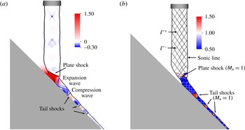
An overview of the mean flow is provided in figure 2(a). The time-averaged pressure distribution is visualized with coloured contours, and a solid contour line is used for the sonic line. The compression and expansion wave patterns are schematically displayed. By time averaging the unsteady flow, the gradients are significantly smoothed out. A weak Mach diamond structure downstream of the nozzle exit is present and it is caused by the mild overexpansion, as discussed in § 2. The pressure averaged over the nozzle exit area is approximately
 $0.5\,\%$
below the reference atmospheric pressure. For noise source identification using the causality method, it is important to keep in mind that the Mach diamond structure moves due to unsteadiness in the flow field. It was decided to use an ‘ideally’ or ‘perfectly’ expanded jet because the current study as well as prior investigations is concerned with the interaction of the turbulent jet with the plate shock and its downstream development. In the presence of a more pronounced Mach diamond structure, the local flow conditions at the impingement location vary greatly depending on the relative location in the jet structure (Henderson et al.
Reference Henderson, Bridges and Wernet2005). In addition, a strong interaction of the large coherent flow structures with the Mach cone structure is expected. Hence, the complexity of the jet-impingement problem is greatly reduced by employing a perfectly expanded jet flow.
Mean flow visualization in the
 $(y,z)$
-plane at
 $x=0$
. (a) Colour contours of the mean pressure field,
 $(p-p_{ref})/p_{ref}$
, the black solid line displays the sonic line, and schematic detailing the structure of compression and expansion waves. (b) Colour contours of normal Mach number
 $M_{n}$
with black lines for
 $M_{n}=1$
and
 ${\it\Gamma}^{\pm }$
marking characteristics.

The shock structures in the impingement region and in the wall jet were identified using a shock identification method based on the normal Mach number discussed in Lovely & Haimes (Reference Lovely and Haimes1999),
 $$\begin{eqnarray}M_{n}=\frac{\boldsymbol{M}\boldsymbol{\cdot }\boldsymbol{{\rm\nabla}}p}{|\boldsymbol{{\rm\nabla}}p|}=\frac{\boldsymbol{v}\boldsymbol{\cdot }\boldsymbol{{\rm\nabla}}p}{a|\boldsymbol{{\rm\nabla}}p|},\end{eqnarray}$$
where
 $\boldsymbol{M}$
is the Mach number vector in the direction of the local flow velocity vector
 $\boldsymbol{v}$
and
 $a$
is the local speed of sound. Normal Mach number isocontours are shown in figure 2(b) (starting slightly above the plate shock). Additionally, a black solid line marks
 $M_{n}=1$
contour lines to highlight possible shock locations. It should be noted that the isocontours need to be interpreted carefully because only isocontours of
 $M_{n}=1$
, where
 $M_{n}$
varies from supersonic (
 $M_{n}>1$
) to subsonic (
 $M_{n}<1$
), are shock locations (Lovely & Haimes Reference Lovely and Haimes1999). The normal Mach number contours identify an impingement plate shock and a shock train downstream of the primary impingement location. The interaction of the turbulent jet with these shock structures induces significant pressure oscillations which are believed to be relevant for noise generation. Moreover, solid (black/white) lines are used to portray characteristics inside the supersonic jet denoted by
 ${\it\Gamma}^{\pm }$
. The characteristics were obtained with the method of characteristics applied to the linearized compressible small-disturbance potential equation utilizing the Prandtl–Glauert transformation.
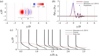
For the purposes of validating the current computational approach, the time-averaged wall pressure distribution is compared with the limited available experimental data by Nakanishi et al. (Reference Nakanishi, Okamoto, Teramoto, Okunuki and Tsutsumi2012) and Akamine et al. (Reference Akamine, Nakanishi, Okamoto, Teramoto, Okunuki and Tsutsumi2014). The time-averaged pressure distribution comprises two regions, A and B, as marked in figure 3(a). The large pressure values in region A are associated with the plate shock. Tail shocks are observed in region B downstream of the plate shock, causing oscillations in the pressure distribution. The peak in the surface pressure distribution extracted at the centreline shown in figure 3(b) is slightly off centre, located at
 $y/D=0.1{-}0.11$
. This result corresponds well with
 $y/D\approx 0.1$
reported by Tsutsumi et al. (Reference Tsutsumi, Takaki, Nakanishi, Okamoto and Teramoto2014). The near-field flow measurements reported in Akamine et al. (Reference Akamine, Nakanishi, Okamoto, Teramoto, Okunuki and Tsutsumi2014) are only available at a few pressure sensor locations placed at the wall, shown in figure 3(b) as solid square symbols. The maximum pressure in the jet-impingement region matches the computational fluid dynamics (CFD) data by Tsutsumi et al. (Reference Tsutsumi, Takaki, Nakanishi, Okamoto and Teramoto2014), with
 ${\rm\Delta}p_{ave}/p_{ref}\approx 2.63$
. Assuming isentropic expansion, the stagnation pressure on the plate would be
 ${\rm\Delta}p_{ave}/p_{ref}\approx 1.67$
. The formation of the plate shock raises the maximum pressure on the wall by roughly
 $36\,\%$
. The velocity profiles in the wall jet are compared with previous hybrid RANS/LES simulations by Housman et al. (Reference Housman, Brehm and Kiris2013). Good agreement of the wall-normal velocity profiles between the two simulations is obtained on considerably different computational grids and by utilizing different simulation strategies. Neither one of the two CFD approaches compared in figure 3 employed wall-resolved LES due to the large computational resources that would be required for such a simulation. A wall-resolved LES may provide some additional insight into the relevance of near-wall unsteadiness and possible separation on the wall as observed by Honda et al. (Reference Honda, Nonomura, Fujii and Yamamoto2011) and Nagata et al. (Reference Nagata, Nonomura, Fujii and Yamamoto2013) for a lower Reynolds number.
(a) Contours of the time-averaged gauge pressure on the impingement plane and (b) comparison of the pressure distribution with experimental data. The experimental data are digitized from Tsutsumi et al. (Reference Tsutsumi, Takaki, Nakanishi, Okamoto and Teramoto2014). (c) Comparison of wall-normal velocity profiles in the wall jet with the hybrid RANS/LES simulation by Housman et al. (Reference Housman, Brehm and Kiris2013). The sonic line is shown as a dashed line.

3.2 Unsteady flow visualization
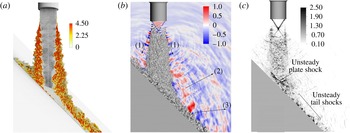
Instantaneous flow visualization of a turbulent jet impinging on a
 $45^{\circ }$
inclined plate in the
 $(y,z)$
-cut-plane: (a) passive trace particle visualization coloured by vorticity magnitude, (b) isocontour of
 $Q$
-criterion,
 $QD/V_{ref}=1.2\times 10^{5}$
, and normalized gauge-pressure contours and (c) greyscale contours of dilatation.

The following discussion is concerned with characterizing the turbulent jet upstream of the impingement location, the jet–plate interaction and the particularities of the unsteady wall jet containing tail shocks. A wide range of relevant temporal and spatial scales can be observed from the passive trace particle visualization (coloured by vorticity) and the
 $Q$
-criterion isocontour surface (with
 $QD/V_{ref}=1.2\times 10^{5}$
) in figure 4(a,b). The unsteady plate and tail shocks can be identified in the dilatation contours in figure 4(c). Fine-grained turbulence and small turbulent eddies organized in large-scale coherent flow structures are visible. Due to the short plate-to-nozzle distance, large levels of vorticity are mainly concentrated in the jet and wall jet shear layers. A general idea about the wave-propagation pattern can be obtained in the normalized gauge-pressure contours in the
 $(y,z)$
-cut-plane in figure 4(b). At least three distinct wave directivities are apparent. The wave fronts emitted by the turbulent jet shear layer (marked with arrows and labelled ‘(1)’) have been carefully studied in the literature for free jets. Tam et al. (Reference Tam, Viswanathan, Ahuja and Panda2008) provided a simple model for the generation of these acoustic waves. The large-scale coherent flow structures may be regarded as a wavy wall moving with supersonic speed past the ambient air, thus emitting Mach waves.
The flow visualizations in figure 4(b,c) clearly depict Mach radiation from large-scale coherent flow structures in the turbulent jet upstream of the impingement location. It is assumed that noise generation from fine-scale turbulence is also present for the current setting. However, the wave fronts are diffused in figure 4(b,c) because the generated noise is nearly omnidirectional, as noted by Tam et al. (Reference Tam, Viswanathan, Ahuja and Panda2008). The two additional types of wave-propagation patterns marked in figure 4(b) have been previously observed by other researchers (see Nonomura et al. Reference Nonomura, Goto and Fujii2011; Nakanishi et al. Reference Nakanishi, Okamoto, Teramoto, Okunuki and Tsutsumi2012; Tsutsumi et al. Reference Tsutsumi, Takaki, Nakanishi, Okamoto and Teramoto2014). The wave fronts ‘(2)’ appear to be emitted from the jet-impingement region and the wave fronts ‘(3)’ seem to originate from the unsteadiness in the wall jet. The relevant physical mechanisms governing the generation of these acoustic waves are, however, not well understood at this point.
3.3 Unsteady flow features: from nozzle exit to impingement point
The vortical flow structures shown in figure 4(b) are initially obliquely aligned to the jet axis. The initial low-amplitude disturbances downstream of the nozzle lip rapidly reach large amplitudes where they saturate and higher modes are nonlinearly generated (or through secondary, tertiary, etc. instability mechanisms). The exact nature of the transition process is not analysed here but some estimates are provided below. Further breakdown of the jet into small-scale structures can be observed in figure 4(b), where the flow field in the shear-layer region is assumed to be ‘fully turbulent’ approximately
 $1D$
downstream of the nozzle exit. The appearance of small-scale turbulent eddies in the instantaneous flow visualization in figure 4(a–c) indicates that the current simulation approach is able to capture the ‘second transition’ of the jet, as it was referred to by Shur et al. (Reference Shur, Spalart and Strelets2005a
,Reference Shur, Spalart and Strelets
b
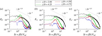
). Additional evidence is provided by analysing the power spectra of different disturbance flow quantities in figure 5(a–c). Ideally, the state of the boundary layer at the nozzle exit would contain resolved turbulence which enters the jet flow in the shear layer (resolution requirements are out of reach for the current Reynolds number). Due to the strong shear-layer instability mechanism, the flow is quickly transitioning in the shear layer. This seems acceptable considering that the instabilities and turbulence are much stronger in the shear layer than in the boundary layer.
Power spectra of flow quantities (a)
 $p^{\prime }=(p-\overline{p})/p_{ref}$
, (b)
 $v_{r}^{\prime }=(v_{r}-\overline{v}_{r})/V_{ref}$
and (c)
 $w^{\prime }=(w-\overline{w})/V_{ref}$
extracted at sample points on the shear-layer line in figure 1(b). It should be noted that the spectra were smoothed to ease the comparison of the data.

Figure 5(a–c) displays the spectral energy
 $E$
of normalized disturbance pressure
 $p^{\prime }=(p-\langle p\rangle )/p_{ref}$
and disturbance velocities
 $v_{r}^{\prime }=(v_{r}-\langle v_{r}\rangle )/V_{ref}$
and
 $w^{\prime }=(w-\langle w\rangle )/V_{ref}$
at four different locations in the shear layer of the jet. The point probes are located at four vertical positions, i.e.
 $z/D=4.75$
,
 $4.50$
,
 $4.25$
and
 $2.00$
, on the shear-layer line right below the lip of the nozzle exit displayed in figure 1(b). Two dashed lines have been added which correspond to the theoretically expected asymptotic behaviour of a turbulent flow in the inertial subrange with
 $E\sim St^{-5/3}$
and the dissipation range with
 $E\sim St^{-7}$
of the von Kármán energy spectrum (Pope Reference Pope2000). The initial high-frequency peak at
 $St\approx 30$
decays quickly in the downstream direction. The cause of this high-frequency peak, whether it is numerical or physical, is not clear at this point. It can be disregarded since it did not seem to play a major role in the current study. This conjecture was scrutinized by comparing the current results with other (Tsutsumi et al.
Reference Tsutsumi, Takaki, Nakanishi, Okamoto and Teramoto2014) and lower-resolution simulations (Brehm et al.
Reference Brehm, Sozer, Moini-Yekta, Housman, Barad, Kiris, Vu and Parlier2013).
According to Michalke (Reference Michalke1984), the largest amplification rates in the jet shear layer are expected for frequencies around
 $St=O(1)$
(and
 $St\approx 2{-}3$
with a phase speed of
 $v_{ph}/V_{ref}\approx 0.6{-}0.7$
for the helical mode with
 $k_{{\it\phi}}=1$
) due to the aforementioned Kelvin–Helmholtz (K–H) type instability mechanism. The dominant frequencies in the initial shear layer observed in the current simulations are within the range of the most amplified frequencies in a round free jet estimated by linear stability theory (see Michalke Reference Michalke1984). By computing the shear-layer thickness of the mean flow and considering the stability analysis results by Michalke (Reference Michalke1984), the region of unstable K–H modes contains frequencies up to approximately
 $St\approx 4{-}6$
(for
 $k_{{\it\phi}}=1$
) for
 $z/D=4{-}5$
. For the current Mach number, it is expected that the helical mode with
 $k_{{\it\phi}}=1$
is more amplified than the axisymmetric mode with
 $k_{{\it\phi}}=0$
. The initial oblique alignment of the
 $Q$
-criterion isosurface in figure 4(b), slightly downstream of the nozzle lip, supports this conjecture. The space–time resolution in the present simulation was based on the estimated relevant frequency range that is needed to resolve the initial shear-layer breakdown. Indeed, a comparison of the spectra in figure 5(a–c) for different grid resolutions (Brehm et al.
Reference Brehm, Sozer, Moini-Yekta, Housman, Barad, Kiris, Vu and Parlier2013) indicates that the present ILES is able to capture the initial growth of the primary instability waves correctly as well as the subsequent breakdown of the flow to turbulence.
The disturbance flow energy spectra for
 $1<z/D<4$
are basically identical to the spectra at
 $z/D=2$
in terms of their asymptotic behaviour. For the current grid resolution, the inertial subrange in the von Kármán energy spectrum following the asymptotic behaviour with
 $f^{-5/3}$
seems to be well established. Hence, from this location (
 $z/D\approx 4$
) forward (with
 $z/D$
decreasing towards the impingement plate) the flow in the shear layer may be considered to be fully turbulent. In the dissipation range with the
 $f^{-7}$
asymptotic behaviour, most of the turbulent kinetic energy is supposed to be dissipated by the physical action of the molecular viscosity. For the current not fully resolved simulations (not DNS), it is assumed that most of the dissipation is actually introduced by the numerical scheme acting as a filter to the unresolved scales and not by the physical action of the molecular viscosity. Comparison of the spectra in figure 5(a–c) with spectra from lower-grid-resolution simulations in Brehm et al. (Reference Brehm, Sozer, Moini-Yekta, Housman, Barad, Kiris, Vu and Parlier2013) suggests that the energy spectra are resolved for up to roughly
 $St=6$
, well into the frequency range relevant here. The simulation accuracy is further validated in § 4 by comparing the acoustic noise signature in the far field with acoustic measurements by Akamine et al. (Reference Akamine, Nakanishi, Okamoto, Teramoto, Okunuki and Tsutsumi2014). Assuming a normal-mode representation of turbulent fluctuations based on LST, one could assume that the disturbance flow spectra are identical for all flow quantities. It is well known, and indeed Panda et al. (Reference Panda, Seasholtz and Elam2005) demonstrated, however, that the normal-mode assumption is not necessarily a good assumption for fully turbulent jet flows. An obvious difference in the spectra is that
 $E_{w^{\prime }}$
contains more energy in the lower-frequency range (
 $St<1$
) than
 $E_{v_{r}^{\prime }}$
and
 $E_{p^{\prime }}$
.
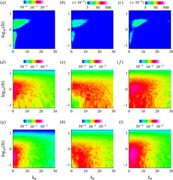
Spectral energy distribution versus Strouhal frequency,
 $St$
, and azimuthal wavenumber,
 $k_{{\it\phi}}$
, for different jet-axis locations
 $z/D=4.5$
,
 $3.0$
and
 $1.0$
((a–c), (d–f) and (g–i)) and flow quantities
 $p^{\prime }$
,
 $v_{r}^{\prime }$
and
 $w^{\prime }$
((a,d,g), (b,e,h) and (c,f,i)).

As the turbulent jet evolves, the unsteady flow goes through significant changes with respect to frequency and azimuthal wavenumber content. In the next step, the three-dimensional nature of the flow field was analysed by applying a double Fourier transform in time and azimuthal direction
 ${\it\phi}$
. To perform these transforms, the unsteady flow data were recorded on
 $20$
circles centred around the jet axis with a radius
 $r/D=0.5$
, as shown in figure 1(b). Each circle contained
 $200$
equispaced sample points. Figure 6 displays the spectral energy content for the disturbance flow quantities at three vertical positions
 $z/D=4.5$
,
 $3.0$
and
 $1.0$
. It should be noted that
 $St$
is plotted on a logarithmic scale, and for this analysis the radial velocity,
 $v_{r}^{\prime }$
, was used. The characteristics of the unsteady flow field between the nozzle exit and the impingement plate can be roughly divided into three regions: (i) transitional shear layer (
 $5\geqslant z/D>4$
), (ii) turbulent jet flow (
 $4\geqslant z/D>1.5$
) and (iii) impingement region (
 $z/D\leqslant 1.5$
). These three regions can be characterized by their particular frequency and wavenumber spectra in figure 6. The transitional jet flow (figure 6
a–c) is dominated by frequencies
 $St=O(1)$
and azimuthal wavenumbers up to roughly
 $k_{{\it\phi}}=10$
. As one may expect for a Mach
 $1.8$
cold jet (Michalke Reference Michalke1984), the oblique modes
 $k_{{\it\phi}}>0$
appear to be initially more amplified than the axisymmetric mode
 $k_{{\it\phi}}=0$
. All spectra also display a region with large amplitudes for low frequencies (
 $0.1<St<0.8$
) and low azimuthal wavenumbers. Further downstream, the spectra broaden, in both frequency and azimuthal wavenumber space. The spectral energy distribution for
 $z/D=3$
is ‘typical’ for the spectral energy distributions of the turbulent jet in region (ii). Distinct differences can be observed between the spectra of disturbance pressure and disturbance velocities with respect to the azimuthal wavenumber content. The energy spectra of the disturbance velocities are dominated by a wider range of azimuthal wavenumbers (up to
 $k_{{\it\phi}}\approx 20$
) in comparison to the energy spectrum of the disturbance pressure (up to
 $k_{{\it\phi}}\approx 10$
). The power spectrum for
 $w^{\prime }$
contains more low-frequency content at low azimuthal wavenumbers than
 $E_{p^{\prime }}$
and
 $E_{v_{r}^{\prime }}$
. With decreasing distance to the plate, the spectral energy shifts towards lower frequencies for all flow quantities, whereby the differences in the spectral wavenumber content remain. Slightly upstream of the impingement location (figure 6
g–i), where the turbulent jet interacts with the oblique plate shock, all three energy spectra,
 $E_{p^{\prime }}$
,
 $E_{v_{r}^{\prime }}$
and
 $E_{w^{\prime }}$
, are dominated by low frequencies with
 $St<1$
and lower azimuthal wavenumbers than upstream. The
 $E_{v_{r}^{\prime }}$
spectrum peaks at larger azimuthal wavenumbers than the
 $E_{p^{\prime }}$
and
 $E_{w^{\prime }}$
spectra. The shift towards lower azimuthal wavenumbers at
 $z/D=1.0$
may be partially explained by the fact that the circle cuts through the impingement region. It shows that the effects of the inclined plate can be felt over a significant distance upstream of the impingement point. The differences in the Fourier spectra are very subtle, and we will demonstrate that the employment of auto-correlation functions is advantageous to distinguish particularities in the unsteady time signals for the different flow quantities.
In the following temporal correlation analysis, three important aspects for characterizing the unsteady flow field between the nozzle exit (
 $z/D=5$
) and the impingement location (
 $z/D=0$
on the centreline) are investigated: (i) temporal (and derived streamwise) length scales of the disturbance flow quantities, (ii) disparity in scales between the shear layer, jet axis and in the vicinity of the plate shock, and (iii) the relationship between different disturbance flow quantities. To understand the noise generation mechanisms, it is important to identify the relevant scales in the different regions of the flow field as well as how the flow quantities are interconnected in the process. Due to the nonlinear nature of the Navier–Stokes equations, it may not be expected that individual flow quantities can be isolated in this process because a coupling between these quantities will probably occur. However, in the following analysis, it will be demonstrated that the dominant temporal scales in the disturbance velocities and pressure can be different in the vicinity of the plate shock.
The dominant scales in the flow field were analysed by computing the temporal auto-correlation function of the different disturbance flow quantities,
 $\boldsymbol{q}^{\prime }(\boldsymbol{x},t)$
, where
 $q_{n}^{\prime }(\boldsymbol{x},t)$
is the
 $n$
th component of the primitive variable vector
 $\boldsymbol{q}^{\prime }=[p^{\prime },v_{r}^{\prime },v_{{\it\Theta}}^{\prime },w^{\prime },T^{\prime }]^{\text{T}}$
recorded at location
 $\boldsymbol{x}$
. For a free jet, Tam et al. (Reference Tam, Viswanathan, Ahuja and Panda2008) employed a similar strategy to identify the coherence time scale that is associated with far-field acoustic noise in the upstream and sideline directions due to small-scale turbulence and in the downstream direction due to Mach radiation. The normalized auto-correlation function,
 $C_{q_{n}^{\prime },q_{n}^{\prime }}^{0}$
, is given by
 $$\begin{eqnarray}C_{q_{n}^{\prime },q_{n}^{\prime }}^{0}({\it\tau})=\frac{\langle q_{n}^{\prime }(t+{\it\tau});q_{n}^{\prime }(t)\rangle }{\langle q_{n}^{\prime }(t)^{2}\rangle }.\end{eqnarray}$$
Throughout this paper,
 $\langle \,\rangle$
denotes time averaging and the superscript
 $0$
is used for normalized correlation functions. The auto-correlation function is merely the Fourier transform of spectra of the disturbance flow quantities,
 $q_{n}^{\prime }$
. Furthermore, according to Tam et al. (Reference Tam, Viswanathan, Ahuja and Panda2008), a coherence time scale can be associated with the shape of the auto-correlation function. In this work, the integral temporal scales,
 $T_{q_{n}^{\prime }}$
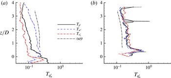
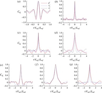
in figure 7(a,b), were obtained by integrating the auto-correlation functions in figure 8. The plots in figure 8 present the auto-correlation functions at particular streamwise locations upstream of the impingement location. Assuming Taylor’s hypothesis, this coherence time scale can also be converted into a physical length scale using an appropriate propagation speed.
Integral temporal scales along (a) the shear-layer line and (b) the centreline. The smoothed data are shown with thick lines and the original data with thin lines.

Auto-correlation functions of disturbance pressure,
 $v_{r}^{\prime }$
velocity and
 $w^{\prime }$
velocity for sample points in the shear layer (a–d) and on the centreline (e–g) of the jet: (a)
 $z/D=4.50$
, (b)
 $z/D=2$
, (c)
 $z/D=0.20$
, (d)
 $z/D=0.25$
, (e)
 $z/D=2$
, (f)
 $z/D=0.46$
, (g)
 $z/D=0.15$
.

The auto-correlation functions for all disturbance flow quantities are very similar close to the nozzle exit, displaying deep undershoots. The deep negative peaks in the auto-correlation function for all flow quantities are typical features (or imprints) of large coherent flow structures in the transitional jet flow, as explained in Tam et al. (Reference Tam, Viswanathan, Ahuja and Panda2008). Further downstream, due to the randomization of the time signals, the initial deep undershoot disappears as the jet shear layer progresses further through the ‘second transition’ process and ultimately breaks down to turbulence. Upstream of the impingement region, the temporal integral scale
 $T_{w^{\prime }}$
is always larger than
 $T_{v_{r}^{\prime }}$
and
 $T_{p^{\prime }}$
in the shear layer. Once the turbulent jet flow reaches the jet-impingement region (
 $z/D=0.20$
and
 $-0.25$
), the interaction of the unsteady jet with the plate shock causes significant changes in the physical scales. The integral temporal scales
 $T_{p^{\prime }}$
and
 $T_{v_{r}^{\prime }}$
increase in the vicinity of the plate shock while
 $T_{w^{\prime }}$
decreases;
 $T_{v_{r}^{\prime }}$
approaches the value of
 $T_{w^{\prime }}$
below the plate shock. The large disparity in the temporal scales for the time signals of the velocity and pressure fields below the plate shock suggests that in this region, the pressure and velocity fields are dictated by widely different physical scales, possibly indicating anisotropies in the flow or even decoupling of flow quantities. A likely explanation of the disparity in scales between the velocity and pressure fields is provided in § 3.4. It will be shown in § 3.4 that the wall jet contains coherent flow structures as well as a stationary mode mostly perceivable in the pressure field spatially extending from the impingement region to the tail shocks in the wall jet.
Next, the differences between the unsteadiness in the shear-layer region and the centre of the turbulent jet are analysed. In § 5, we utilize this information to explain why stronger normalized correlations are obtained in the turbulent jet core than in the shear layer. Based on prior research studies for free jets (by, for example, Panda & Seasholtz Reference Panda and Seasholtz2002; Panda et al.
Reference Panda, Seasholtz and Elam2005; Bogey & Bailly Reference Bogey and Bailly2007; Tam et al.
Reference Tam, Viswanathan, Ahuja and Panda2008), the flow features in the jet centre and inside the shear layer can be expected to be different. These differences are aggravated for the impinging jet analysed here because the potential core length of an equivalent free jet (
 ${\rm\Delta}z_{c}/D\approx 8$
) is larger than the actual plate-to-nozzle distance. Therefore, the turbulence originating in the shear-layer region cannot penetrate into the centre of the jet before impinging on the inclined plate. The integral temporal scales for all flow quantities in the jet core are very similar until the jet reaches the impingement region. Hence, it appears that the disturbance flow quantities are closely related to each other. Assuming a nearly constant propagation speed of the dominant flow structures at the centreline, it seems that the integral scales along the centreline scale perfectly with the momentum thickness,
 ${\it\theta}$
, of the jet.
At
 $z/D=2.0$
, the auto-correlation functions in the centre,
 $y/D=0$
, and in the shear layer,
 $y/D=0.5$
, display some differences. The disturbance flow field in the jet centre appears to be more coherent, which can be noted by larger undershoots right next to the peak. The increased temporal integral scales
 $T_{v_{r}^{\prime }}$
and
 $T_{p^{\prime }}$
in the jet core indicate larger temporal coherence for
 $v_{r}^{\prime }$
and
 $p^{\prime }$
in the centre of the jet. The integral temporal scales rise significantly around the location of the plate shock (
 $z/D=0.40$
). Right above the impingement plate,
 $z/D=0.15$
,
 $C_{v_{r}^{\prime },v_{r}^{\prime }}^{0}$
displays a significantly smaller width of the peak, and thus a smaller integral time scale, than
 $C_{p^{\prime },p^{\prime }}^{0}$
. It should be noted that we repeated the analysis of the disturbance flow field along a line with a
 ${\rm\Delta}y/D=0.1$
offset to centreline and obtained nearly identical results. In this way any possible artefacts that may only occur just in the centre of the jet could be excluded. The key finding of this discussion is that the integral temporal scales and relationships between the different disturbance flow quantities are widely different along the jet centreline and the shear-layer line.
Space–time plots of the streamwise disturbance velocity along (a) the shear-layer line and (b) the jet axis, as shown figure 1(b). (c) Instantaneous snapshot of the shock indicator function in the symmetry plane displaying weak shocks in the core of the jet.

The space–time (or
 $(z,t)$
) plots in figure 9(a,b) for the streamwise disturbance velocity are used to determine the propagation speeds in the core,
 $v_{p,c}$
, and shear layer,
 $v_{p,s}$
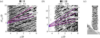
, of the jet. The widely different patterns in the space–time plots are another indicator for the differences in temporal scales in the core and the shear layer of the jet. The following discussion is aimed at obtaining an understanding of the unsteady nature of the flow in the jet shear layer and the jet core. The propagation speed of the most dominant flow features can be estimated by following a peak (light grey region) or valley (black region) in the
 $(z,t)$
plots. Dashed lines have been added which visualize the propagation speed of the most dominant flow features, the backward travelling acoustic wave with
 $v_{a}^{-}=1-a_{ref}/V_{ref}=0.44$
and the jet exit velocity,
 $V_{e}=V_{ref}$
. The most dominant flow features inside the shear layer propagate significantly faster than along the jet axis. The coherent flow structures inside the shear layer propagate supersonically with approximately
 $v_{p,s}=0.69V_{ref}$
, where the speed of sound is approximately
 $a=0.56V_{ref}$
. The estimated propagation speed of roughly
 $v_{p,c}=0.34V_{ref}$
in the centre of the jet is shown as a dashed line in figure 9(b). In flow visualizations of a planar jet by Shariff & Manning (Reference Shariff and Manning2013) employing ray tracing, fine-scale features inside the jet can be identified to travel significantly slower than the coherent flow structures in the shear layer. Based on the propagation speed of the dominant flow features in the centre of the jet (
 $v_{p,c}<v_{a}^{-}$
) in figure 9(b), it is, however, unlikely that these flow features are associated with (backward travelling) acoustic waves. Although it is theoretically possible that an interference pattern of acoustic waves travels faster than the speed of sound, it is more likely that small shock structures propagate inside the jet. In figure 9(c), the shock identification method of Lovely & Haimes (Reference Lovely and Haimes1999) was used to visualize possible shock locations inside the jet. Equation (3.1) was extended to account for unsteadiness (the movement of the shocks). Greyscale contours of the normal Mach number
 $M_{n}$
are shown in figure 9(c). Small shock structures appear to originate at the edge of the shear layer and propagate to the centre of the jet. Estimation of the speeds of these shock structures utilizing simple shock relations produces velocities that are very close to the previously estimated propagation speed of roughly
 $v_{p,c}=0.34V_{ref}$
.
3.4 Unsteady flow features: wall jet
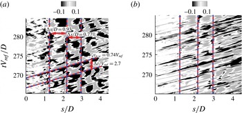
Space–time plots of (a) disturbance pressure and (b) streamwise velocity fluctuations extracted along streamline 1 in figure 1(b). The vertical lines mark the approximate locations of the tail shocks.

The role of the large-scale coherent flow structures in the wall jet is explored here. Upstream of jet impingement, Mach radiation is clearly emitted by supersonically convecting large-scale structures, as can be seen in figure 4(b,c). Previously, it was assumed that the interaction of these flow structures with the plate shock and the solid wall defines their predominant role in the noise generation process. The flow visualizations in figure 4(a–c) indicate, however, that large structures persist in the wall jet past the impingement region. It remains to be shown whether these flow structures propagate downstream supersonically relative to the ambient medium and, thereby, are also able to emit Mach radiation. Further, the interaction of these flow structures with the tail shocks may provide an additional mechanism for the generation of sound waves. These two-noise sources are assumed to be different with respect to their particular wave-propagation pattern. While the acoustic waves generated by coherent flow structures are mainly directional, the unsteady shock motion generates more omnidirectional wave patterns.
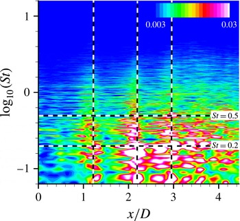
The FFT amplitude of
 $p^{\prime }$
along sampling line 3. The vertical lines mark the approximate locations of the tail shocks.

Figure 10 shows space–time (
 $s,t$
) plots of disturbance pressure and streamwise velocity fluctuations along a streamline in the wall jet with arclength
 $s$
(see figure 1
b). In the
 $(s,t)$
plots of disturbance pressure, the imprints from the tail shocks are clearly visible and the mean tail shock positions are marked with vertical dashed lines. For the streamlines further away from the wall (not shown), these distinct features are progressively less pronounced. The tail shock interaction with the unsteady flow is less visible in the
 $(s,t)$
plots for streamwise disturbance velocity. The velocity field is less affected by the presence of the tail shocks. Figure 10(a,b) can provide some possible clues about the expected frequency content of the emitted acoustic waves from the shear-layer shock train interaction. The dominant spacings of the streaks in the streamwise disturbance velocity pattern that can be attributed to dominant flow features are fairly constant, with
 ${\rm\Delta}tV_{ref}/D\approx 2.7$
. This would lead to an interaction frequency of
 $St\approx 0.38$
for the shear-layer (single) tail shock interaction. Further, the spacings of the tail shocks introduce another frequency scale considering that the tail shocks are being distorted by the unsteady shear layer. Assuming a propagation speed of the coherent flow structures in the wall jet of
 $v_{p,w}=0.74$
and approximating the distances
 $L_{1,2}=0.93$
(between tail shocks 1 and 2) and
 $L_{2,3}=0.77$
(between tail shocks 2 and 3), this interaction frequency can be estimated as
 $St\approx 0.8$
–1. This is clearly a simplified view because the shear-layer shock train interactions are more complicated and nonlinear in nature, providing a broader frequency content. A better estimate of the frequency content associated with the tail shock oscillations is obtained by applying a Fourier transform to the pressure field in the wall jet. Figure 11 shows the fast Fourier transform (FFT) amplitude of
 $p^{\prime }$
along sampling line 3. Large Fourier amplitudes are shown around the tail shocks (marked with vertical dashed lines). As expected, the unsteady tail shocks contain a wide spectrum of frequencies. The largest amplitudes are, however, obtained for low Strouhal numbers.
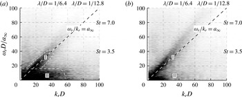
The space–time plots provide mainly a qualitative description of the flow features. A more quantitative analysis of the unsteady flow features in the wall jet is obtained by computing the frequency–wavenumber spectra. The spectra contain information about the wave phase speeds (
 $v_{p}={\it\omega}/k$
) and modal characteristics inside the unsteady wall jet. The frequency–wavenumber spectra for disturbance pressure and streamwise disturbance velocity are displayed in figure 12(a,b). The plots were generated by placing sample points on a streamline following the wall jet (in figure 1
b) and applying a double Fourier transform in time and streamwise direction to the disturbance flow quantities. To reduce spectral leakage, a windowing function was utilized similar to the one used in Freund (Reference Freund2001). The windowing function follows as
 $$\begin{eqnarray}w(s)=\frac{1}{2}\left(\tanh \left(5\frac{s_{1}-s}{s_{s}-s_{1}}\right)+\tanh \left(5\frac{s_{2}-s}{s_{e}-s_{2}}\right)\right),\end{eqnarray}$$
where
 $s_{s}$
and
 $s_{e}$
define the first and last points on the sampling line, and
 $s_{1}$
and
 $s_{2}$
were chosen so that the solution was ramped over the first and last
 $5\,\%$
of the total length of the sampling line. Two distinct regions can be identified in the spectra for disturbance pressure. Region ‘I’ contains the propagating part of the solution. Region ‘II’ is associated with a non-propagating (
 $\text{d}s/\text{d}t=0$
) part of the solution, and may be linked to the unsteady shock structure above the wall that is quasistationary in space (standing wave). While region II extends over a large area in the frequency–wavenumber spectra for the disturbance pressure, it is less present in the disturbance velocity spectra. In § 3.3, we showed that the auto-correlation functions of the disturbance pressure and velocity fields are significantly different in the impingement region. Region II is associated with the unsteady shock structure and, therefore, becomes more visible in pressure.
Frequency–wavenumber spectra for (a) disturbance pressure and (b) disturbance velocity fluctuations extracted along streamline 1 in figure 1(b).

The main motivation for computing the frequency–wavenumber spectra is that we can extract information about which parts of the solution are radiating and non-radiating. The wave equation has the important property that the part of the solution with
 ${\it\omega}>0$
and a real wavenumber
 $k$
(in the propagation direction) can only be acoustically radiating if the frequency and the wavenumber follow the inequality
 $|k|<{\it\omega}/a_{\infty }$
. Hence, only the fraction in the spectrum above the dashed line following the equation
 ${\it\omega}D/a_{\infty }=k_{r}D$
can be part of the acoustically radiating solution. A large portion of the spectra are evanescent pressure waves that are negligible a few wavelengths away from the source region without an associated sound field. The analysis seems to support the fact that the wall jet contains coherent flow structures that travel supersonically and thereby emit Mach radiation. The current analysis purely accounts for sound generation in the mean streamline propagation direction. It is likely, however, that the unsteady shock structures mainly generate sound radiation in directions that are not aligned with the mean streamline. The fact that a large fraction of the frequency–wavenumber pairs associated with the unsteady shock structure are located in the non-radiating part of the spectrum does not downplay their importance for the noise generation process originating from the wall jet. From the analysis of the noise generation mechanisms in underexpanded supersonic jets, it is known that sound waves emanate from the terminal locations of shock waves in the shear layer. In contrast to Mach radiation originating from large-scale coherent structures convecting supersonically, which has a dominant directivity, these sound waves appear to be more omnidirectional, spreading out almost spherically from the point of generation. Thus, only a very small fraction of the shock noise (in the direction of the wavenumber vector) can be captured in the current frequency–wavenumber analysis.
3.5 Proper orthogonal decomposition
Application of POD results in a decomposition of the flow field into a set of basis functions which represents most of the flow energy, as defined by a user-defined energy norm, with the least number of modes (Lumley Reference Lumley, Yaglom and Tatarsky1967). For many fluid dynamics applications, POD has been used to identify the most energetic flow structures. At this point, it must be noted, however, that it is not guaranteed that existing POD modes have dynamical significance. Therefore, the POD analysis results need to be carefully interpreted. For example, Freund & Colonius (Reference Freund and Colonius2002) applied POD to a Mach 0.9 turbulent jet. They alluded to the fact that the radiated sound from turbulence amounts to a very small fraction of the total energy. Hence, a POD approach in the temporal domain may not be able to capture the physics of the radiated sound waves. Furthermore, beforehand it is not necessarily clear which energy norm should be used to capture the relevant flow physics. Freund & Colonius (Reference Freund and Colonius2002) found that the efficiency of representing the flow data depends strongly upon the norm used and which data are represented. When analysing the acoustic field, it may be advantageous to follow an approach similar to the one described in Suzuki et al. (Reference Suzuki, Bodony, Ryu and Lele2007). Instead of using snapshots in time, Suzuki et al. (Reference Suzuki, Bodony, Ryu and Lele2007) used Fourier coefficients as snapshots for the POD. Suzuki et al. (Reference Suzuki, Bodony, Ryu and Lele2007) argued that this approach is preferable for acoustics because the acoustic waves contain much less energy than the turbulent jet or the unsteady shock structures. In the current study, POD is applied in the temporal domain since we are mainly interested in analysing the coherence in the source region. The spectral energy content of the different POD modes can be retained from the time coefficients. The spectra can be compared with the far-field noise signature, and thus we can infer information about the relative importance of the most energetic flow structures with respect to the sound field produced. The reader is referred to appendix A for details about the current implementation of the POD method.
3.5.1 Proper orthogonal decomposition results
To properly interpret the POD results, it is important to establish what type of information about the relevant flow physics this mathematical construct is able to attain. A single POD mode that is composed of the mode shape function and time coefficient can be viewed as a global mode ansatz in the form
 $\hat{{\it\phi}}(\boldsymbol{x})\exp (\text{i}{\it\omega}t)$
, where
 $\hat{{\it\phi}}$
and
 ${\it\omega}$
are generally complex. In the context of POD analysis, however, we exclude any type of growing or decaying solutions in time, i.e.
 ${\it\omega}\in \mathbb{C}$
, because it is assumed that we are dealing with statistically stationary processes, and in this sense a temporal equilibrium has been reached, i.e.
 ${\it\omega}\in \mathbb{R}$
. The key limitation for a single POD mode is that the solution is essentially spatially stationary. Noting that in their most simplistic form, large-scale coherent flow structures can be described by a travelling wave ansatz in the form
 $u(x,t)\propto \exp (\text{i}(kx-{\it\omega}t))$
, where the wave amplitude changes in time (here,
 ${\it\omega}\in \mathbb{R}$
) are omitted for the aforementioned reason. This means that at least two POD modes are required in order to mathematically describe a travelling wave in terms of POD. This also is the reason why POD modes frequently occur in pairs. Thus, the basic physical phenomena relevant to the current flow problem, i.e. shock oscillations, large-scale coherent flow structures, acoustic waves and their interactions, cannot be captured by a single POD mode and the dynamics is imprinted onto several modes.
The most energetic POD modes, with mode 1 to mode 3 ((a,d,g), (b,e,h), (c,f,i)) considering different energy norms based on pressure (a–c), entropy fluctuation term (d–f) and kinetic disturbance energy (g–i): (a)
 $p^{\prime (1)}$
, (b)
 $p^{\prime (2)}$
, (c)
 $p^{\prime (3)}$
, (d)
 $s^{\prime (1)}$
, (e)
 $s^{\prime (2)}$
, (f)
 $s^{\prime (3)}$
, (g)
 $K^{\prime (1)}$
, (h)
 $K^{\prime (2)}$
, (i)
 $K^{\prime (3)}$
. Colour contours of the projected pressure field are shown outside the source region.

The fraction of total energy captured by the first
 $m$
POD modes in terms of the coherence factor shown as solid, dashed and dashed-dotted lines and the
 $n$
th eigenvalue shown as square, circular and triangle symbols.

Figure 13(a–i) displays the three most energetic POD modes for three energy norms considering the disturbance pressure,
 $p^{\prime }$
, the entropy fluctuation term,
 $s^{\prime }$
, and the kinetic disturbance energy,
 $K^{\prime }$
. The POD mode energy distributions are shown as greyscale contours and the colour contours denote the pressure field outside the source region. The pressure field associated with the POD mode is obtained by projecting the unsteady pressure data onto the right eigenvectors in equation (A 2). To provide an idea about the propagation direction in the pressure field away from the source region, we added dotted lines marking four observation angles of
 ${\it\Theta}=75^{\circ }$
,
 $90^{\circ }$
,
 $105^{\circ }$
and
 $120^{\circ }$
. The POD mode shapes for the different energy norms differ significantly and, thus, they appear to capture particular flow features in the unsteady source region. The pressure POD modes mainly highlight the dynamics of the unsteady plate shock. The POD mode shapes provide some similarities with the shock structure in the instantaneous visualization of dilatation in figure 4(b). The dominant motion of the shock structures may be inferred by considering the different pressure POD mode shapes. Qualitatively, the shock can be assumed to move back and forth between two opposing peaks in the pressure POD mode. The interpretation is clearly limited due to the fact that the overall motion is a superposition of several POD modes. For vertical jet impingement, the interpretation of the shock motion is more straightforward, as discussed in Brehm et al. (Reference Brehm, Sozer, Moini-Yekta, Housman, Barad, Kiris, Vu and Parlier2013). Smaller amplitudes of the pressure POD mode are also detected in the supersonic flow region of the wall jet.
The POD modes based on the energy norm considering the entropy fluctuation term display large amplitudes in the jet shear layer extending into the impingement region. The mode shapes appear to capture the interaction of the coherent flow structures with the solid wall. The dominant wavelength of these flow structures can be roughly estimated by the streamwise distance between two consecutive peaks in mode shapes. Assuming a propagation speed of
 $v_{p}/V_{ref}=0.69$
extracted in the space–time plots in figure 9(a) and an approximate wavelength of
 ${\it\lambda}/D=1.2$
from the
 $s^{\prime }$
-based POD mode shapes, the frequency
 $St=0.58$
is close to the peak frequency in the
 $120^{\circ }$
observer direction. The distinct peaks in the wall jet region highlight areas in the flow of increased unsteadiness in the tail shock structure. The
 $s^{\prime }$
-based POD modes appear to identify an interaction of coherent flow structures with the tail shocks. The most distinguishing feature of the POD mode shapes based on
 $K^{\prime }$
is that they accentuate the shear layer in the turbulent jet extending into the wall jet region. For all POD modes, two dominant pressure wave-propagation directions are apparent. The projected pressure field for the
 $s^{\prime }$
-based POD modes seems to be dominant in the
 ${\it\Theta}=100^{\circ }{-}120^{\circ }$
observer direction. For the
 $K^{\prime }$
-based POD modes, a larger wavelength and a different propagation pattern emerge with predominantly lower propagation angles.
In order to measure the coherence in the flow field we introduce the coherence factor
 ${\it\psi}_{m}$
. The coherence factor provides a measure of how the energy is distributed over the different POD modes:
 $$\begin{eqnarray}{\it\psi}_{m}=\left.\left(\mathop{\sum }_{n=1}^{m}{\it\lambda}^{n}\right)\right/\left(\mathop{\sum }_{n=1}^{M_{tot}}{\it\lambda}^{n}\right),\end{eqnarray}$$
where
 ${\it\lambda}^{n}$
is the
 $n$
th eigenvalue of the eigenvalue problem described in (A 3),
 $M_{tot}$
is the total number of POD modes and
 $m\leqslant M_{tot}$
. For a free turbulent jet, a significant number of POD modes (in the temporal domain) are required to capture a large amount of the energy in the unsteady flow field. Due to the impingement of the jet involving large fluctuation amplitudes in the impingement region, the coherence of the flow field is significantly increased. A large amount of energy of the disturbance flow field is contained within the impingement region. Figure 14 illustrates that the coherence in the flow field depends strongly on the choice of the energy norm. The pressure-based POD modes show significantly stronger coherence than for the other two energy norms. While the first
 $50$
pressure POD modes capture
 $70\,\%$
of the flow energy, approximately
 $75$
and
 $110$
POD modes are needed to capture the same amount of energy for the
 $K^{\prime }$
- and
 $s^{\prime }$
-based energy norms. For the entropy-based energy norm, the energy is most evenly distributed over the different POD modes.
Discrete Fourier transform of the POD time coefficients for the three most energetic POD modes considering different energy norms based on (a) pressure,
 $p^{\prime }$
, (b) entropy,
 $s^{\prime }$
, and (c) kinetic disturbance energy,
 $K^{\prime }$
.

Lastly, it remains to analyse the temporal characteristics of the POD modes. The time coefficients in (A 5) are Fourier transformed in time and the spectra are displayed in figure 15(a–c). It should be noted that the Fourier spectra were smoothed to ease the comparison of the data, and the original data are shown in the background with grey lines. The Fourier coefficients are normalized with the largest Fourier coefficient in the spectrum of the original data set (grey solid lines). For all chosen energy norms, the maxima in the Fourier spectra generally shift towards higher frequencies with increasing mode number (
 $n>10$
) (quickly filling up the entire frequency range in figure 15). The time-spectral characteristics of the most energetic POD modes are distinctly different depending on the choice of the energy norm. Whereas the time coefficients of the three most energetic POD modes of the entropy term peak around
 $St=0.4{-}0.6$
, the time coefficients for turbulent kinetic disturbance energy contain large amplitudes for lower Strouhal numbers. The Fourier transformed time coefficients for the pressure-based POD modes do not show a clear trend. While modes
 $1$
and
 $2$
display maximum Fourier amplitudes at around
 $St=0.4{-}0.5$
, mode 3 displays a low-frequency peak. An interesting finding is that the peaks in the spectra of the time coefficients for turbulent kinetic disturbance energy at low frequencies and the entropy fluctuation term at
 $St\approx 0.5$
appear to coincide with the dominant frequencies for the two maxima at
 ${\it\Theta}=75^{\circ }$
and
 ${\it\Theta}=120^{\circ }$
in the far-field OASPL in figure 16(b).
4 Acoustic wave-propagation pattern
Noise source identification relies on the fact that the radiated sound field contains features that can be linked to flow characteristics in the noise source region. Hence, the current objective is to carefully analyse the far-field sound signature and trace it back into the source region. While § 3 was concerned with the unsteady nonlinear flow in the source region, here we will study the near-field and far-field acoustic features, while mainly focusing on the directivity pattern. Furthermore, experimental data are available for validating our numerical simulation approach.
4.1 Far-field acoustic noise predictions
First, our computational results are compared with far-field acoustic noise measurements by Nakanishi et al. (Reference Nakanishi, Okamoto, Teramoto, Okunuki and Tsutsumi2012). The acoustic data comparison was performed at six microphone locations,
 $40D$
away from the impingement location, as shown in figure 16. Here, the Ffowcs-Williams and Hawking (FW–H) integral method was utilized to propagate the unsteady flow data in the near field from the permeable surfaces (acoustic control surface) to the six microphone locations in the far field. The FW–H method was chosen over the Kirchhoff method because the FW–H method is less sensitive to nonlinearities at the control surface. A more detailed discussion of this approach and the acoustic control surface selection is provided in Housman et al. (Reference Housman, Brehm and Kiris2013). To study surface scattering effects, we also computed the noise field with a linear acoustic scattering code based on the equivalent source method presented in Kiris et al. (Reference Kiris, Barad, Housman, Sozer, Brehm and Moini-Yekta2014) and Brehm et al. (Reference Brehm, Housman, Kiris and Hutcheson2015c
). It was found that the results were insensitive to surface scattering effects provided that the correct location for the acoustic surface was chosen. The different permeable surfaces and the far-field sample locations are shown in figure 16(a). The far-field predictions are based on flow field information on the selected FW–H surfaces. Hence, it is important to construct an FW–H surface suitable for this purpose. It is crucial to avoid a large contribution from hydrodynamic pressure fluctuations on the permeable surfaces. The placement of the FW–H surface is based on a widely used practice discussed in Liu et al. (Reference Liu, Corrigan, Kailasanath, Heeb, Munday and Gutmark2014). Considering the FW–H equation, it can be shown (see Lyrintzis Reference Lyrintzis2003) that when the surfaces are placed in the near-field region where
 $\hat{p}^{\prime }\sim 1/r(x)$
the far-field predictions will converge (here,
 $r(x)$
is the local radius on the FW–H surface and
 $\hat{p}^{\prime }$
is the pressure fluctuation intensity).
(a) The permeable surfaces used in the FW–H method and the far-field sample locations. (b) The overall acoustic sound pressure levels (OASPLs) extracted at
 $r=40D$
.

In figure 16(b), the overall acoustic sound pressure level (OASPL) is compared with the experimental data considering four different permeable FW–H surfaces displayed in figure 16(a). The temporal Fourier transforms were computed using five windows with
 $T\approx 120D/V_{ref}$
and 50 % overlap. Hanning windowing was applied to reduce spectral leakage and accumulated noise in the spectra. Two distinct local maxima can be identified in the OASPL distribution. The first maximum occurs at roughly
 $75^{\circ }$
and may be associated with noise generated from the deflected wall jet. The second local maximum occurs at roughly
 $120^{\circ }$
and is mainly associated with pressure waves originating in the jet-impingement region. Surface 1 is clearly too small to capture all of the important dynamics in the wall jet region, thus the first maximum at
 $75^{\circ }$
is underpredicted. The addition of a vertical extension to surface 1 down to the impingement plane (denoted by surface
 $1+2$
) results in a large increase in the OASPL at low observation angles
 ${\it\Theta}$
. This is not surprising and has been observed in many other studies, such as Liu et al. (Reference Liu, Kailasanath, Boris, Heeb, Munday and Gutmark2012, Reference Liu, Corrigan, Kailasanath, Heeb, Munday and Gutmark2014). Surface 2 cuts directly through the deflected turbulent jet flow and is, thereby, contaminated by significant hydrodynamic pressure fluctuations. The significantly larger FW–H surfaces 3 and
 $3+4$
provide similar OASPLs. These results capture the overall trends of the OASPL with respect to the observation angle, albeit at slightly higher noise levels than in experiments. The absolute values are predicted within an acceptable range of
 $\pm 3$
dB.
Power spectral density (PSD) versus Strouhal number at six probe locations with
 $r=40D$
and observation angles of (a)
 ${\it\Theta}=60^{\circ }$
, (b)
 ${\it\Theta}=75^{\circ }$
, (c)
 ${\it\Theta}=90^{\circ }$
, (d)
 ${\it\Theta}=105^{\circ }$
, (e)
 ${\it\Theta}=120^{\circ }$
and (f)
 ${\it\Theta}=135^{\circ }$
.

In addition to the OASPL, a comparison of the power spectral density (PSD) at the same six far-field point probes is presented in figure 17(a–f). The PSD is defined as
 $$\begin{eqnarray}L_{p}=20\log _{10}(\hat{p}/(f_{min}p_{a}))[\text{d}B/St],\end{eqnarray}$$
where
 $p_{a}=20~{\rm\mu}\text{Pa}$
is the audible reference pressure,
 $f_{min}=1/T$
is the lowest frequency in the sample,
 $T$
is the length of the time interval and
 $\hat{p}$
is the pressure Fourier amplitude at the sensor location. The FW–H surface
 $3+4$
in figure 16(b) was used for the present results. The data were smoothed to remove large oscillations. The CFD results compare well with the experimental far-field measurements for all observation angles. For smaller observation angles (
 ${\it\Theta}=75^{\circ }$
and
 $90^{\circ }$
), the maximum in the SPL distributions occurs at smaller Strouhal numbers than for larger observation angles (
 ${\it\Theta}=105^{\circ },120^{\circ }$
and
 $135^{\circ }$
). For the two most dominant propagation directions, i.e.
 ${\it\Theta}=75^{\circ }$
and
 ${\it\Theta}=120^{\circ }$
, the maxima occur at two distinct frequencies,
 $St\approx 0.2$
and
 $St\approx 0.5$
respectively.
Although the universal spectra of Tam et al. (Reference Tam, Golebiowski and Seiner1996) were only validated for free jets, it appears that these spectra can be employed to match the data at
 $75^{\circ }$
and
 $120^{\circ }$
. It should be noted that for these two spectra the main contribution comes from the F-spectrum at low frequencies. The G-spectrum is, however, required to obtain the correct decay for high frequencies. The best match of the spectrum at
 $75^{\circ }$
was obtained when using different peak frequencies for the F-spectrum,
 $St_{F}=0.22$
, and the G-spectrum,
 $St_{G}=0.55$
. It must also be noted that the local peak in the spectrum at
 $90^{\circ }$
cannot be recovered using these two spectra, similarly to peaks in the spectra associated with shock noise presented in Tam et al. (Reference Tam, Golebiowski and Seiner1996).
The validated results provide great confidence that our computational simulation approach is able to capture the key physical mechanisms responsible for noise generation in the nonlinear flow region enclosed by the FW–H surfaces. The current predictions of the far-field noise signature exceed the prediction accuracy provided by previous high-fidelity simulations of the same flow field by Tsutsumi et al. (Reference Tsutsumi, Takaki, Nakanishi, Okamoto and Teramoto2014). The improved prediction accuracy of our results may be attributed to increased grid resolution and the use of numerical schemes with lower numerical dissipation.
The magnitude of the Fourier coefficients (in SPLs) for four octave-banded frequencies,
 $St=0.16$
,
 $0.33$
,
 $0.66$
and
 $1.31$
(a–d).

4.2 Near-field acoustic noise analysis
The noise-propagation pattern in the near field was analysed by computing temporal Fourier transforms of the unsteady pressure field in the
 $(y,z)$
-plane with
 $x=0$
. The magnitude (in SPLs) and phase (in radians) of the complex Fourier coefficients are shown in figures 18 and 19, which portray a general idea about the noise source distribution and the wave-propagation pattern. The apparent wave fronts in the phase plots and fluctuation intensity in the SPL contours clearly point towards two pre-eminent noise source regions: the jet-impingement region and the wall jet. One needs to be very careful when interpreting SPL and phase plots. Phase plots, for example, are insensitive to the wave amplitude. Although clear wave fronts may emerge in the phase plots, they can be associated with low-amplitude waves. Further, phase plots do not discriminate against acoustic and, for example, evanescent or hydrodynamic instability waves. Tracing the wave fronts back to possible noise sources may also be problematic considering that the radiated sound experiences refraction due to high gradients in the velocity and density fields. Lastly, an important well-known issue of noise source identification is that measurement of the acoustic field outside the source region is not sufficient to uniquely determine the acoustic sources (Rienstra & Hirschberg Reference Rienstra and Hirschberg2004). This issue is addressed in more detail in the following section when introducing the causality approach. In the context of noise source identification, the spectral analysis of the acoustic near field provides information that will be explored to guide the placement of observer locations for the causality approach in § 5. In order to obtain a sensible cause and effect relationship between the source region and the two distinct maxima observed in the OASPL in figure 16(b), the observer locations (also referred to as field points) must be placed in regions where we can clearly separate the physical mechanisms responsible for the two predominant noise-propagation directions.
The SPL contours are shown in figure 18(a–d) for four octave-banded frequencies
 $St=0.16$
,
 $0.33$
,
 $0.66$
and
 $1.31$
(with centre frequency
 $St_{0}=0.041$
). For higher frequencies, the sharp decay in the SPL can be attributed to the coarsening grid far away from the source region. The largest amplitudes in the near field are observed for
 $St=0.33$
and
 $St=0.65$
. Arrows have been added to roughly identify distinct near-field source regions that may be associated with different noise generation mechanisms. It is highly unlikely that distinct noise sources have similar directional dependence (Tam et al.
Reference Tam, Viswanathan, Ahuja and Panda2008). Nevertheless, it can be expected that some of the regions in the SPL plots are partially overlapping in certain areas. Based on the shape of the SPL contours, at least three distinct regions of noise generation can be identified, i.e. the shear layer of the turbulent jet (1), the jet-impingement region (2) and the wall jet (3). For high frequencies, Mach radiation from the turbulent jet (1) upstream of the impingement plane propagates downstream, and some radiation originating from the wall jet (3) can be identified. The unsteadiness at the inception of the shear layer is dominated by high frequencies, and the SPL contours spread away from the shear layer. In § 3.3, it was shown that further downstream lower frequencies become increasingly more dominant. For
 $St=0.33$
and
 $St=0.66$
, the SPL contours display two distinct maxima expanding out from the impingement region (2) and the unsteadiness in the wall jet (3). The pre-eminent noise sources are suspected to be located in these two regions. For the smallest octave-band frequency shown here,
 $St=0.16$
, the second maximum in the SPL contours, associated with the impingement region, almost disappears and the noise from the wall jet region becomes the dominant noise contributor.
Phase plots for four frequencies,
 $St=0.16$
,
 $0.33$
,
 $0.66$
and
 $1.31$
(a–d).

Phase plots are used to unveil the directivity pattern of the acoustic pressure waves outside the source region. The phase plots in figure 19(a–d) are obtained at the centre frequencies that were used for the SPL plots. The phase angles are displayed in radians, varying from
 $-{\rm\pi}$
to
 ${\rm\pi}$
with a black–white–black colour map. Different types of waves, such as acoustic, vorticity, entropy, etc., can be identified in the phase plots. Dashed lines and arrows have been added to highlight the directivity of the wave fronts. Although refraction is captured in this analysis, it is not straightforward to determine the actual acoustic noise source regions from these plots. It is generally not clear whether the phase contours in the source regions are associated with purely acoustic pressure waves or other waves, such as vorticity waves, entropy waves, etc. For low Strouhal numbers (
 $St=0.16$
and
 $St=0.33$
), the phase contour lines continuously extend in a wide arc into the wall jet. Thus, it can be conjectured that the noise generated in the impingement region appears to be phase-locked to the noise originating from the wall jet for these frequencies. In the intermediate frequency range (
 $St=0.33$
and
 $St=0.66$
), black dashed lines mark wedges that may be associated with different acoustic sources. In figure 19(d), wave fronts within the unsteady jet shear layer are clearly visible for
 $St=1.31$
. These wave fronts are almost perpendicular to the sonic line of the mean flow, implying that these waves propagate downstream with the mean flow inside the shear layer. It must be noted that the instability waves in the transitional jet close to the nozzle lip are not clearly distinguishable from the acoustic sound waves once they reach larger amplitudes. These vortical flow structures with a dominant frequency around
 $St=O(1)$
generate acoustic waves by travelling supersonic past the ambient air. The acoustic speed of the ambient fluid is close to the phase speed of the dominant flow structures. The plate and tail shock oscillations on the impingement plate cannot easily be identified in the phase plot because they do not behave like a travelling wave and do not contain a pronounced propagation direction. The POD analysis in § 3.5 was able to capture the dynamics of the shocks.
5 Noise source identification
In order to identify the dominant noise sources and reveal the relevant physical mechanisms responsible for noise generation it is not sufficient to separately analyse the flow dynamics in the source region and the radiated acoustic sound field. The key to obtaining an in depth understanding of the noise generation mechanisms is to link the dynamics of the unsteady flow field discussed in § 3 to the features in the radiated sound field discussed in § 4. Simultaneous visualization of the instantaneous flow and acoustic fields can provide an idea of which specific events are responsible for noise generation, see for example Hileman & Samimy (Reference Hileman and Samimy2001), Bogey & Bailly (Reference Bogey and Bailly2003) and Hileman et al. (Reference Hileman, Thurow, Caraballo and Samimy2005). In the current study, however, we employ a different approach by using the causality method. Appendix B provides additional background information about the causality method as it was employed in this paper. In summary, the causality method relies on computing cross-correlations between flow quantities inside the jet-impingement flow field and the radiated acoustic pressure outside the nonlinear flow regime. An attractive feature of this method is that the effects of scattering, absorption and refraction on sound radiation are automatically included by virtue of simultaneously extracting information from both the flow and acoustic fields.
Although noise generation has been studied in great detail for free jets, the available literature on noise source identification lacks studies targeting jet-impingement noise. The current approach follows in the steps of many previous investigations (Panda & Seasholtz Reference Panda and Seasholtz2002; Panda et al.
Reference Panda, Seasholtz and Elam2005; Bogey & Bailly Reference Bogey and Bailly2007; Liu et al.
Reference Liu, Corrigan, Kailasanath, Heeb, Munday and Gutmark2014) utilizing the causality method for the identification of noise sources in a turbulent free jet, but we apply it to the jet-impingement problem. It is clear that the contributions from unsteady fluctuations on the surface (accounted for by the surface integral in (B 3)) are non-negligible for jet impingement. In contrast to the volume term, which represents acoustic quadrupoles, the surface integral term involves only one derivative and, therefore, represents acoustic dipoles. In addition, the contribution of the second term in Lighthill’s stress tensor, namely the entropy fluctuation term
 $p^{\prime }-a_{\infty }^{2}{\it\rho}^{\prime }$
, is assumed to be significant for supersonic jet impingement since it involves unsteady shock structures. This term is, however, difficult to obtain experimentally because two thermodynamic quantities need to be measured independently. This is one of the reasons why the entropy fluctuation term has not been thoroughly studied. A differentiation is made between normalized and non-normalized correlations. Previous studies employing the causality approach (see, for example, Bogey & Bailly Reference Bogey and Bailly2007; Liu et al.
Reference Liu, Corrigan, Kailasanath, Heeb, Munday and Gutmark2014) have not elaborated on the importance of their differentiation. Indeed, we expand on some thoughts put forward on this matter by Panda (Reference Panda2005). He clarifies that simply utilizing normalized correlations may lead to an incorrect interpretation of the noise source distribution. In the current paper, we follow the physical expectation that by employing non-normalized correlation functions, the strongest fluctuations can be differentiated as the source and the weaker fluctuations as the effect (Panda Reference Panda2005).
5.1 Normalized cross-correlations
The normalized cross-correlation functions
 $C^{0}$
(where the superscript
 $0$
denotes the normalization) provide valuable information about the interplay of vortical flow structures with the unsteady shocks and solid surface, which leads to significant hydrodynamic pressure fluctuations and the generation of acoustic waves. In order to differentiate between shear and self-noise, the stress tensor is decomposed into its first- and higher-order contributions,
 $$\begin{eqnarray}\langle {\it\rho}V_{r}^{2};p^{\prime }\rangle =\langle 2\langle {\it\rho}\rangle \langle V_{r}\rangle V_{r}^{\prime };p^{\prime }\rangle +\langle {\it\rho}^{\prime }\langle V_{r}\rangle ^{2};p^{\prime }\rangle +\langle 2\langle V_{r}\rangle {\it\rho}^{\prime }V_{r}^{\prime };p^{\prime }\rangle +\langle \langle {\it\rho}\rangle V_{r}^{\prime 2};p^{\prime }\rangle +\langle {\it\rho}^{\prime }V_{r}^{\prime 2};p^{\prime }\rangle ,\end{eqnarray}$$
where
 ${\it\rho}=\langle {\it\rho}\rangle +{\it\rho}^{\prime }$
and the fluctuating part of the velocity component in the observer direction is
 $V_{r}^{\prime }=V_{r}-\langle V_{r}\rangle$
. It should be noted that approximation of Lighthill’s stress tensor in the form
 ${\it\rho}u_{i}u_{j}\approx \langle {\it\rho}\rangle u_{i}u_{j}$
by neglecting density fluctuations is reasonable for low-speed unheated flows. For the current high-speed turbulent jet flow impinging on an inclined plate, density fluctuations are inherent to the physics. Thus, all terms in Lighthill’s stress tensor contain a non-negligible dependence on density. The flow quantities in the source region, such as
 ${\it\rho}^{\prime }$
,
 $V_{r}^{\prime }$
and
 $p^{\prime }$
, are normalized with
 ${\it\rho}_{ref}$
,
 $V_{ref}$
and
 ${\it\rho}_{ref}V_{ref}^{2}$
respectively. The far-field acoustic pressure is normalized with
 ${\it\rho}_{\infty }a_{\infty }^{2}$
, as is common in the traditional acoustic analogy approach, where
 ${\it\rho}_{\infty }$
and
 $a_{\infty }$
are the ambient density and speed of sound outside the source region. Before computing the cross-correlation functions, the signals were bandpass filtered with
 $St_{low}=0.05$
and
 $St_{high}=4$
.
Colour contours of peak normalized cross-correlation with the observer point in the
 ${\it\Theta}=120^{\circ }$
direction and contour lines of time delay with solid lines for
 ${\it\tau}>0$
and dashed lines for
 ${\it\tau}<0$
: (a)
 $C_{p^{\prime },p^{\prime }}^{0}$
, (b)
 $C_{p^{\prime },V_{r}^{\prime }}^{0}$
, (c)
 $C_{p^{\prime },s^{\prime }}^{0}$
.

In order to impart a clear interpretation of the results, we computed the peak normalized cross-correlation functions for the different components of Lighthill’s stress tensor in the entire
 $(y,z)$
-plane (see figure 20) instead of limiting ourselves to sample points and lines (as in previous works). The employment of the spatial distribution of the peak normalized cross-correlation function eases the way for an improved interpretation of the results. It is important to keep in mind that regions with large values of the peak normalized cross-correlation function do not inevitably identify acoustic source regions. They highlight parts of the flow field where the unsteady flow features, irrespective of their amplitudes, strongly correlate with the acoustic pressure at the observer location. This information can be utilized to obtain a physical understanding of how the noise is being generated. In this context, it seems clear that the large-scale coherent flow structures convecting with the turbulent jet, before interacting with the shock structures or the solid surface, are not able to directly generate noise that is detectable upstream of the jet flow direction, for example at an observation angle of
 ${\it\Theta}=120^{\circ }$
.
The peak normalized cross-correlation functions for the first-order and entropy fluctuation terms are visualized in figure 20(a–c). Solid (
 ${\it\tau}>0$
) and dashed (
 ${\it\tau}<0$
) contour lines of the time delay
 ${\it\tau}$
are used to portray the propagation direction of the fluctuating flow quantities that are highly correlated with the acoustic pressure. For the cross-correlation study, two field points were placed outside the LES region with a radial distance to the impingement location of
 $r/D=5$
and observation angles of
 ${\it\Theta}=75^{\circ }$
and
 $120^{\circ }$
relative to the jet axis. The field points were placed in a region where the grid resolution is still sufficient to support the relevant frequency range. A solid circle (
 $\bullet$
) is used to mark the position of the observer location in the flow field (see figures 20 and 21). The chosen observer angles correspond to the two angles where the local maxima in the OASPL were observed in § 4. Further, the two observer locations were placed in the two distinct regions with large SPLs in figure 18(a–d) of the acoustic near field (see § 4.2), where the two acoustic noise signatures associated with noise sources in the impingement and wall jet regions can be virtually separated. Although the two point probes were placed much closer to the source region than the far-field sensors, the spectra display very similar characteristics to the far-field spectra. Nakanishi et al. (Reference Nakanishi, Okamoto, Teramoto, Okunuki and Tsutsumi2012) also confirmed experimentally that the acoustic spectra at
 $r/D=15$
and
 $r/D=40$
are similar to each other.
Colour contours of peak normalized cross-correlation with the observer point in the
 ${\it\Theta}=75^{\circ }$
direction and contour lines of time delay with solid lines for
 ${\it\tau}>0$
and dashed lines for
 ${\it\tau}<0$
: (a)
 $C_{p^{\prime },p^{\prime }}^{0}$
, (b)
 $C_{p^{\prime },V_{r}^{\prime }}^{0}$
, (c)
 $C_{p^{\prime },s^{\prime }}^{0}$
.

Away from the immediate source region, the distribution of the peak normalized cross-correlation function
 $C_{p^{\prime },p^{\prime }}^{0}$
as shown in figure 20(a) provides a depiction of how the acoustic waves propagate away from the source region. As one may expect, the acoustic pressure correlates well in a large area sufficiently far away from the source region, and the distances between the time-delay contour lines are fairly constant, implying wave propagation with
 $a_{\infty }$
. The region where the noise is generated can be estimated by tracing the contour lines of time delay back into the source region. Dashed lines have been added to mark the area (or wedge) with large correlations outside the source region. Interestingly, the regions with high fluctuation intensities (in the source region) obtain small values of the normalized cross-correlation function. Although large fluctuations are generated in the source region, a large portion of this unsteadiness is not acoustically radiating.
For all three normalized cross-correlation functions displayed in figure 20(a–c), large correlations are obtained inside the turbulent jet. The alignment of the time-delay contour lines provides information about the propagation direction of the highly correlated flow features. A small illustration has been added in figure 20(b), highlighting the propagation direction. The highlighted region is assumed to propagate in the direction of decreasing time delays normal to the contour lines of time delay. The abrupt changes in the peak correlation functions
 $C_{p^{\prime },p^{\prime }}^{0}$
and
 $C_{p^{\prime },s^{\prime }}^{0}$
follow the directions of the characteristics that are visualized in figure 20(a). The abrupt changes of regions of large
 $C_{p^{\prime },p^{\prime }}^{0}$
and
 $C_{p^{\prime },s^{\prime }}^{0}$
(aligned with characteristics) are probably associated with an interaction of the flow features inside the jet with the weak Mach diamond structure. It should be noted that the particular shapes of these regions are not sufficiently statistically converged to allow for a more detailed interpretation.
For the observer point in the
 ${\it\Theta}=120^{\circ }$
direction, the largest correlation values are realized in the centre of the jet for
 $V_{r}^{\prime }$
. The region of large
 $C_{p^{\prime },V_{r}^{\prime }}^{0}$
stretches over a significant streamwise extent of roughly
 $2D$
. Large correlation values are detected even downstream of the plate shock after an abrupt reduction of
 $C_{p^{\prime },V_{r}^{\prime }}^{0}$
in the vicinity of the plate shock. For a free turbulent jet, Bogey & Bailly (Reference Bogey and Bailly2007) observed large values of the correlation function at the end of the potential core region. They used this and additional flow visualization to conjecture that the noise generation mechanism for the downstream jet-noise component is linked to periodic and intermittent intrusion of vortical structures into the jet core. We are following a similar train of thought here. The current data support the presumption that large coherent structures with a coherence length comparable to the diameter of the jet are indirectly detectable (through normalized cross-correlation) in the jet centre. The obvious conjecture is that these flow structures interact with the solid wall as well as the plate shock, causing large fluctuations of Lighthill’s stress tensor and pressure fluctuations on the impingement plate.
Significantly lower correlations are observed towards the edges of the jet in the shear layer. The radial dependence of the peak normalized cross-correlations with the velocity fluctuations agrees with similar observations from other studies considering free jets (see, for example, Panda et al.
Reference Panda, Seasholtz and Elam2005; Bogey & Bailly Reference Bogey and Bailly2007). Various explanations for the radial dependence of the cross-correlation function are plausible. From prior studies by Panda & Seasholtz (Reference Panda and Seasholtz2002) and Tsutsumi et al. (Reference Tsutsumi, Takaki, Nakanishi, Okamoto and Teramoto2014) considering a free jet with the same flow conditions, it is known that the potential core length extends over roughly
 $8D$
downstream of the nozzle exit. Because the plate-to-nozzle distance is only
 $5D$
, the turbulence initiated in the shear layer does not contaminate the entire jet cross-section before jet impingement. Therefore, the shear layer containing highly energetic vortical flow structures consists of a richer frequency spectrum (see also § 3) than the jet centre, resulting in a strong decorrelation between the time signals in the jet shear layer and the acoustic far field. In an analysis utilizing correlation functions, it is common to point towards regions with large correlation values. However, an interesting observation here is that for the entropy fluctuation term, distinct regions of very low correlation appear at the edge of the source region. None of the other cross-correlation functions share this distinguishing feature.
For the second observer location in the
 ${\it\Theta}=75^{\circ }$
direction, the cross-correlation function
 $C_{p^{\prime },p^{\prime }}^{0}$
depicted in figure 21(a) clearly indicates that the noise is mainly originating from the wall jet. Large values of
 $C_{p^{\prime },V_{r}^{\prime }}^{0}$
are obtained in the wall jet downstream of the plate shock inside the supersonic flow region. Further, strong correlations with the entropy fluctuation term are obtained at the edge of the shear layer of the wall jet in figure 21(c). The large values of
 $C_{p^{\prime },s^{\prime }}^{0}$
inside the shear layer of the wall jet in figure 21(c) could be linked to coherent flow structures that propagate in the direction of the sonic line. This, however, begs the question of why we did not observe similarly large values of
 $C_{p^{\prime },s^{\prime }}^{0}$
inside the turbulent jet for the first observer point. The strong correlations suggest that these flow features are involved in the generation of noise predominantly observed in the
 ${\it\Theta}=75^{\circ }$
direction. We assume that these strong correlations are not associated with the unsteady shock structures in the wall jet due to the fact that
 $C_{p^{\prime },p^{\prime }}^{0}$
did not display similarly large correlations in this region.
A simple derivation can be used to describe how the entropy fluctuation term can be physically interpreted. We start with a well-known thermodynamic relation
 $$\begin{eqnarray}\frac{\text{D}p}{\text{D}t}=a^{2}\frac{\text{D}{\it\rho}}{\text{D}t}+\frac{\partial p}{\partial s}\bigg|_{{\it\rho}}\frac{\text{D}s}{\text{D}t},\end{eqnarray}$$
where
 $\text{D}/\text{D}t$
represents the material time derivative and
 $s$
is the entropy. Writing equation (5.2) in terms of the disturbance quantities, subtracting
 $\text{D}{\it\rho}^{\prime }/\text{D}t$
from the right- and left-hand sides and introducing the so-called excess density as
 ${\it\rho}_{ex}={\it\rho}^{\prime }-p^{\prime }/a_{\infty }^{2}$
leads to
 $$\begin{eqnarray}-\frac{\partial ^{2}{\it\rho}_{ex}}{\partial t^{2}}=\frac{\partial }{\partial t}\left[\left(\frac{a^{2}}{a_{\infty }^{2}}-1+\frac{{\it\rho}_{e}}{{\it\rho}}\right)\frac{\text{D}{\it\rho}^{\prime }}{\text{D}t}+\frac{{\it\rho}^{2}}{a_{\infty }^{2}}\frac{\partial T}{\partial {\it\rho}}\bigg|_{s}\frac{\text{D}s}{\text{D}t}+\boldsymbol{{\rm\nabla}}\boldsymbol{\cdot }(\boldsymbol{v}{\it\rho}_{e})\right],\end{eqnarray}$$
where the first right-hand side term vanishes for constant heat capacity, as assumed here. It follows that sound is produced though the entropy fluctuation term by spatial density variations (last term) and due to non-isentropic processes (second term), such as large gradients in the shear layer and discontinuities across shock waves. The entropy fluctuations in the shear layer may be related to large gradients in this region. The impingement zone also contains large gradients as well as flow discontinuities that may spawn entropy fluctuations.
Coloured contours of peak normalized cross-correlation
 $C_{p^{\prime },{\it\rho}^{\prime }(V_{r}^{\prime })^{2}}^{0}$
and contour lines of time delay with solid lines for
 ${\it\tau}>0$
and dashed lines for
 ${\it\tau}<0$
: (a)
 $120^{\circ }$
, (b)
 $75^{\circ }$
.

The (normalized) cross-correlation analysis for second-order terms (not shown) demonstrated that the second-order disturbance flow quantities correlate significantly less with acoustic pressure than the first-order disturbance flow quantities. This observation agrees with what was reported for free jets in prior research studies by Panda et al. (Reference Panda, Seasholtz and Elam2005) and Bogey & Bailly (Reference Bogey and Bailly2007). The normalized cross-correlation results for the third-order terms are displayed in figure 22. Correlations of the third-order term are not negligible, which is consistent with observations for free jets by Panda et al. (Reference Panda, Seasholtz and Elam2005). The magnitudes of the peak cross-correlations are, however, not as large as those of the first-order terms. The spatial distribution of
 $C_{p^{\prime },{\it\rho}^{\prime }(V_{r}^{\prime })^{2}}^{0}$
is similar to what was observed for the first-order terms. For the first observation angle of
 ${\it\Theta}=120^{\circ }$
, larger magnitudes of the cross-correlation function are noted in the potential core region of the jet upstream of the plate shock. For the second observation angle of
 ${\it\Theta}=75^{\circ }$
, no regions with large cross-correlations are clearly detectable inside the source region.
5.2 Non-normalized cross-correlations
Based on the causality relation in (B 6), the sound-producing regions in the source region are identified by computing the non-normalized cross-spectral density (or cross-correlation) function between the acoustic pressure in the far field and different parts of Lighthill’s stress tensor. It should be noted that when simply computing Reynolds stresses only regions with large fluctuations are highlighted, but there is no differentiation between sound-producing and ‘silent’ unsteadiness. The following analysis utilizing non-normalized cross-correlation functions, on the other hand, extracts the part of the solution in the source region that is correlated with the acoustic pressure. The first- and higher-order contributions of the source term (integrand of (B 6)) are visualized in figure 23(a–f) considering the field point in the
 ${\it\Theta}=120^{\circ }$
observation direction (marked with ▪). All first-order terms display similar maximum amplitudes, whereas their spatial distributions are distinctly different. Large amplitudes of
 $C_{p^{\prime },V_{r}^{\prime }}$
are observed in the region where the shear layer impinges on the wall as well as in the shear layer itself. The cross-correlation function of the entropy fluctuation term peaks where the shear layer interacts with the plate shock. Interestingly, while
 $C_{p^{\prime },V_{r}^{\prime }}$
peaks in the vicinity of the sonic line,
 $C_{p^{\prime },s^{\prime }}$
peaks closer to the centreline of the turbulent jet. A possible explanation is that
 $C_{p^{\prime },V_{r}^{\prime }}$
captures the interaction of the impinging shear layer with the solid wall and
 $C_{p^{\prime },s^{\prime }}$
captures the interaction with the plate shock. Figure 23(c) displays the source contribution from the pressure term. Although the contribution of the surface integral in (B 5) is visualized in the entire
 $(y,z)$
-plane, it must be noted that only the pressure fluctuations on the solid wall are relevant for the acoustic intensity in the far field (left-hand side of (B 5)). Indeed,
 $C_{p^{\prime },p^{\prime }}$
reaches its maximum on the wall just below the shear-layer impingement point. The higher-order terms shown in figure 23(d–f) reach significantly lower values in comparison to the first-order terms. For all three higher-order terms, the peak amplitudes are obtained right above the impingement plate below the oblique shock. The term
 $C_{p^{\prime },(V_{r}^{\prime })^{2}}$
shows similar features to
 $C_{p^{\prime },V_{r}^{\prime }}$
, while the amplitudes in the shear layer are lower. When including density fluctuations, the third-order term
 $C_{p^{\prime },{\it\rho}^{\prime }(V_{r}^{\prime })^{2}}$
peaks at around the same location as
 $C_{p^{\prime },p^{\prime }}$
.
Colour contours of peak non-normalized cross-correlation for
 $120^{\circ }$
observation angle: (a)
 $C_{p^{\prime },V_{r}^{\prime }}$
, (b)
 $C_{p^{\prime },s^{\prime }}$
, (c)
 $C_{p^{\prime },p^{\prime }}$
, (d)
 $C_{p^{\prime },(V_{r}^{\prime })^{2}}$
, (e)
 $C_{p^{\prime },u^{\prime }v^{\prime }}$
, (f)
 $C_{p^{\prime },{\it\rho}^{\prime }(V_{r}^{\prime })^{2}}$
.

For the sample point in the
 $75^{\circ }$
observation direction, the distributions of the different non-normalized peak cross-correlation functions (not shown here) look almost identical to the results for the sample point in the
 $120^{\circ }$
observation direction. Although the non-normalized cross-correlation function contains information about the linear dependence between two time signals, regions with large fluctuation amplitudes are weighted more strongly than regions with small fluctuation amplitudes, such as the potential core region inside the turbulent jet. This explains why the non-normalized cross-correlation function is less sensitive to the observer location.
An expected finding is that the distributions of the normalized and non-normalized cross-correlation functions are widely different. For example,
 $C_{p^{\prime },V_{r}^{\prime }}^{0}$
displays large amplitudes inside the jet axis (for the first field point), whereas
 $C_{p^{\prime },V_{r}^{\prime }}$
peaks in the shear layer and in the region where the shear layer impinges on the plate. This study demonstrates that the normalized cross-correlation function provides information about how the noise is physically generated, but it does not necessarily highlight the actual source locations. In contrast, the non-normalized cross-correlation function retains information about fluctuation amplitudes in the source region and, therefore, it can be used to detect the noise source distribution. Considering the large fluctuation amplitudes and the low normalized cross-correlation in the impingement region, it is evident that this part of the unsteady flow field is not very efficient in generating sound waves. This is not surprising because only a small fraction of the unsteadiness is contributing to the acoustic field.
6 Discussion
The noise sources and noise generation mechanisms for a perfectly expanded supersonic jet impinging on a
 $45^{\circ }$
inclined plate were investigated by employing a three-step approach. (i) The unsteady flow field was analysed to obtain a detailed understanding of the relevant flow physics in the source region. (ii) The acoustic far-field noise signature was characterized with respect to its wave directivity pattern and frequency content. (iii) The causality approach was used to link the acoustic pressure signature to characteristics in the unsteady source region. The current study is based on numerical simulations which were successfully validated against experimental data, such as far-field noise data and pressure measurements in the source region. Two local maxima were identified in the far-field noise signature in figure 16(b) at
 ${\it\Theta}=75^{\circ }$
and
 ${\it\Theta}=120^{\circ }$
. The PSD plots for
 ${\it\Theta}=75^{\circ }$
and
 ${\it\Theta}=120^{\circ }$
in figure 17(b,e) display peaks around
 $St=0.2$
and
 $St=0.5$
respectively. The SPL plots in figure 18(a–d) provide a rough overview of regions in the flow field where the noise is being generated. For the octave-band frequency of
 $St=0.16$
, only the wall jet region displays large SPL. For larger Strouhal numbers, such as
 $St=0.33$
and
 $St=0.66$
, two regions with elevated SPLs can be found to originate from the jet-impingement region as well as the wall jet.
Schematic illustration of the identified most relevant noise generation mechanisms in the jet-impingement flow.

This study aimed at identifying the most dominant non-compact noise sources. Figure 24 gives a schematic illustration of the most relevant noise generation mechanisms that were identified in the current study. Predominantly omnidirectional radiation from fine-scale turbulent structures observed for turbulent free jets is not included in this schematic. One of the reasons is that the different methods employed here (POD, causality method, etc.) to analyse the unsteady flow field and to conduct noise source identification are not well suited for studying this type of noise source. When reconstructing the acoustic spectra in the
 ${\it\theta}=75^{\circ }$
and
 ${\it\theta}=120^{\circ }$
observer directions it was noted, however, that in order to match the spectra at high frequencies some contribution from the G-spectrum is needed.
The analysis of the unsteady flow field in § 3.2 provided various findings that substantiated the existence of large-scale coherent flow structures in the turbulent jet flow upstream of the impingement plate. For example, the unsteady flow visualization utilizing passive trace particles coloured by vorticity magnitude in figure 4(a) displays an agglomeration of fine-scale eddies convecting together in an organized fashion. Additionally, the strong Mach radiation detectable in the gauge-pressure contours in figure 4(b) provides indirect evidence of the presence of these flow structures. The space–time plot in figure 9(a) shows traces of dominant coherent flow structures in the shear layer which propagate supersonically. As has been analysed in the past for free jets by many researchers, the acoustic waves generated by these large-scale flow structures mainly propagate in the downstream direction. The directional Mach radiation is marked in figure 24 with the label (1) and is in agreement with similar observations by other researchers, such as Honda et al. (Reference Honda, Nonomura, Fujii and Yamamoto2011) and Nagata et al. (Reference Nagata, Nonomura, Fujii and Yamamoto2013).
In the correlation analysis, the presence of the coherent flow structures appears to be detectable inside the potential core region of the jet flow. The integral scales in the jet core (assuming constant propagation speed) seem to scale with the momentum thickness of the shear layer. Most importantly, the normalized cross-correlation function
 $C_{p^{\prime },V_{r}^{\prime }}^{0}$
shows strong correlations with the acoustic pressure in the
 ${\it\Theta}=120^{\circ }$
observer direction in the centre of the turbulent jet over a large streamwise extent of
 $O(D)$
. The strong cross-correlations in the centre of the jet with the acoustic pressure in the
 ${\it\Theta}=120^{\circ }$
observer direction suggest that these flow structures take on an important role in the noise generation predominantly observed at
 ${\it\Theta}=120^{\circ }$
.
In addition to Mach radiation, these vortical flow structures play another important role in the noise generation process for jet impingement. Neglecting effects of compressibility, it can be shown that the source term in Lighthill’s equation (B 1) can be written as
 $\partial \unicode[STIX]{x1D61B}_{ij}/\partial x_{i}\partial x_{j}=\langle {\it\rho}\rangle \boldsymbol{{\rm\nabla}}\boldsymbol{\cdot }(\boldsymbol{v}\times \boldsymbol{w})$
, where
 $\boldsymbol{w}=\boldsymbol{{\rm\nabla}}\times \boldsymbol{v}$
is the vorticity. Considering the simplified version of Lighthill’s stress tensor, the theory of vortex sound (Powell Reference Powell1964; Howe Reference Howe2003) can be used to explain that the impinging vortices generate noise through vortex distortion, such as vortex stretching and tearing. This process is marked in figure 24 with the label (2). Various findings were provided throughout the paper that point to this phenomenon. The strong non-normalized correlations of
 $C_{p^{\prime },V_{r}^{\prime }}$
at the shear-layer impingement point can be partially attributed to the impingement of the highly unsteady shear layer (containing coherent flow structures). Moreover, the
 $s^{\prime }$
-based POD analysis highlighted this region as being highly energetic, and large POD mode amplitudes extend from the shear-layer impingement point into the shear layer. The
 $s^{\prime }$
-based POD mode shapes display wave-like characteristics in this region that are typically observed for coherent flow structures. An interesting finding is that the most energetic
 $s^{\prime }$
-based POD modes display a dominant frequency around
 $St=0.4{-}0.6$
.
The jet-impingement noise problem is very complicated in the way in which the overall noise generation process involves various physical mechanisms. Highly unsteady shock structures were identified in the instantaneous visualization of dilatation contours and by employing a shock identification method by Lovely & Haimes (Reference Lovely and Haimes1999). The shock shear-layer interaction was assumed to play an important role in the noise generation process as reported by Tsutsumi et al. (Reference Tsutsumi, Takaki, Nakanishi, Okamoto and Teramoto2014). The most energetic
 $p^{\prime }$
-based POD modes capture the large pressure fluctuations in the vicinity of the plate shock. Furthermore, the large non-normalized cross-correlations of
 $C_{p^{\prime },s^{\prime }}$
around the plate shock structure point towards significant contributions from shock associated noise. The particular shape of the local maximum in the SPL plot at
 ${\it\Theta}=90^{\circ }$
has some resemblance with peaks associated with shock noise in spectra presented in Tam et al. (Reference Tam, Golebiowski and Seiner1996). The shock oscillations are induced by the motion of the vortical flow structures, making it difficult to effectively isolate shock-induced noise and the aforementioned vortex impingement noise generation mechanisms. In this work, however, we assume that the interaction of the vortical flow structures with the plate shock provides its own noise generation mechanism (denoted by label (3) in figure 24). The arrows schematically illustrate the unsteady motion of the oblique shock that is held responsible for the generation of acoustic pressure waves.
The entropy fluctuation term in Lighthill’s stress tensor is inherently attributed to non-isentropic processes, such as entropy generation across shocks. However, there are other shock-related noise generation mechanisms that can be understood by reconsidering Lighthill’s source term in the presence of flow discontinuities. These flow discontinuities can be accounted for by utilizing the definition of the generalized derivative. In 1D, Lighthill’s stress tensor is a scalar
 $\unicode[STIX]{x1D61B}_{11}$
and the source term can be rewritten as
 $$\begin{eqnarray}\frac{\hat{\partial }^{2}\unicode[STIX]{x1D61B}_{11}}{\partial x^{2}}=\frac{\partial ^{2}\unicode[STIX]{x1D61B}_{11}}{\partial x^{2}}+\frac{\partial }{\partial x}({\rm\Delta}\unicode[STIX]{x1D61B}_{11}{\it\delta}(x-x_{s}))+{\it\Delta}\left(\frac{\partial \unicode[STIX]{x1D61B}_{11}}{\partial x}\right){\it\delta}(x-x_{s}),\end{eqnarray}$$
where
 $\hat{\partial }/\partial x$
is the generalized derivative,
 ${\rm\Delta}\unicode[STIX]{x1D61B}_{11}$
is the jump term in
 $\unicode[STIX]{x1D61B}_{11}$
and
 ${\it\delta}(x-x_{s})$
is the delta function applied at the assumed shock location
 $x_{s}$
. In addition to the original quadrupole term, the modified source term contains unsteady forces in terms of dipoles and mass addition in terms of monopole sources. A detailed theoretical and numerical analysis of the shock noise mechanisms was provided in Meadows (Reference Meadows1997). This analysis demonstrated that all three terms, i.e. monopole, dipole and quadrupole contributions, are potentially important. For the current Mach number and frequency range, it can be assumed that the contribution from the monopole term is most dominant, but also that dipole and quadrupole contributions are not negligible (according to the analysis by Meadows (Reference Meadows1997)). Although only the quadrupole term was included in the application of the causality method, large magnitudes of the other terms in the vicinity of the plate shock can be expected based on the results for the non-normalized cross-correlation functions in figure 23(a–f).
Next, the noise generation mechanisms in the wall jet are discussed. Two main noise generation mechanisms marked by labels (4) and (5) were identified somewhat similarly to previous observations by Honda et al. (Reference Honda, Nonomura, Fujii and Yamamoto2011), Nonomura et al. (Reference Nonomura, Goto and Fujii2011) and Nagata et al. (Reference Nagata, Nonomura, Fujii and Yamamoto2013) for lower Reynolds numbers. Honda et al. (Reference Honda, Nonomura, Fujii and Yamamoto2011), Nonomura et al. (Reference Nonomura, Goto and Fujii2011) and Nagata et al. (Reference Nagata, Nonomura, Fujii and Yamamoto2013) observed shock-induced separation for the same (
 $45^{\circ }$
) and larger impingement angles. For these flow conditions, noise generation from shock-induced separation seemed to play an important role in the noise generation process. These findings could not be confirmed for the current flow conditions with a significantly higher Reynolds number and an impingement angle of
 $45^{\circ }$
. It should be noted that the noise generation mechanism associated with tail shock interaction can be viewed as a separate mechanism from the noise generated through shock-induced separation as it was reported in Honda et al. (Reference Honda, Nonomura, Fujii and Yamamoto2011) and Nagata et al. (Reference Nagata, Nonomura, Fujii and Yamamoto2013). The noise generation mechanism associated with the separation bubble contains unsteadiness that is mainly generated in the shear layers and their interactions. The shock motion, however, may also affect the unsteadiness of the separation bubble. Therefore, a clear distinction between the separation-bubble-induced noise generation mechanism discussed in Honda et al. (Reference Honda, Nonomura, Fujii and Yamamoto2011) and Nagata et al. (Reference Nagata, Nonomura, Fujii and Yamamoto2013) and the noise generation mechanism (4) is non-trivial. For larger impingement angles, unsteady separation and its associated noise generation mechanisms may become important even for higher Reynolds numbers. Various findings support the conjecture that Mach radiation originating from the wall jet shear layer (5) and also the interaction of the coherent flow structure with the tail shock structure (4) provide mechanisms for noise generation. In § 3.2, it was demonstrated that the frequency–wavenumber spectrum for pressure contains a significant fraction that fulfils the radiation condition (region I in figure 12(a,b)). Furthermore, the frequency–wavenumber spectrum shows a second region in figure 12(a,b) that was characterized as a standing wave type solution. This part of the spectrum (region II) contains comparable amplitudes to the propagating part of the solution (region I). The strong coupling in the wall jet complicates matters significantly because the different noise generation mechanisms are highly interconnected. Particular regions in the wall jet were highlighted by different methods to play an important role in the noise generation process. The Fourier transformed pressure signal along a streamline in the wall jet showed large localized peaks around the tail shocks with predominantly low-frequency content. Furthermore, large values of
 $C_{p^{\prime },V_{r}^{\prime }}^{0}$
in figure 20(b) were also detected inside the wall jet below the sonic line. The normalized cross-correlation function
 $C_{p^{\prime },s^{\prime }}^{0}$
in figure 20(c) also showed strong correlations between the acoustic pressure in the
 ${\it\Theta}=75^{\circ }$
observer direction and the entropy fluctuation term in the wall jet around the sonic line.
In the POD analysis, the
 $K^{\prime }$
-based POD mode shapes highlight the shear layers of the jet upstream of the impingement region and a large coherent region in the wall jet. The most energetic
 $K^{\prime }$
-based POD modes are dominated by low-frequency content. The pressure field associated with the most energetic
 $K^{\prime }$
-based POD modes appears to propagate predominantly towards smaller observer angles and they seem to originate from the unsteady wall jet region. The large coherent region of the
 $K^{\prime }$
-based POD modes in the wall jet with low-frequency content may be attributed to the fact that the tail shock structures are closely coupled to the upstream flow conditions which are dictated by the flow conditions at the plate shock. The localized peaks of the most energetic
 $s^{\prime }$
-based POD modes in figure 13(d–f) suggest that they are associated with the interaction of vortical structures in the shear layer and the tail shock structures within the wall jet.
Appendix A. Background on proper orthogonal decomposition
In the current analysis, the snapshot method is utilized. For problems where the spatial dimension,
 $m$
, is much greater than the number of available time steps,
 $N$
, it is more efficient to employ the snapshot method (Sirovich Reference Sirovich1987) for POD. For more details about the POD snapshot method used here, see Chatterjee (Reference Chatterjee2000) for a basic introduction to POD and Rowley (Reference Rowley2001) and Freund & Colonius (Reference Freund and Colonius2002) for details on how it can be applied to fluid dynamics problems. In the current discussion, it is assumed that a vector of flow quantities
 $\boldsymbol{q}(\boldsymbol{x},t)=(p^{\prime },u^{\prime },v^{\prime },w^{\prime },s^{\prime })$
is defined over a region of interest
 ${\it\Omega}$
, and additional weighting factors
 $\boldsymbol{w}$
weight the contribution of the components of
 $\boldsymbol{q}(\boldsymbol{x},t)$
in the vector norm,
 $$\begin{eqnarray}|\boldsymbol{q}|_{{\it\Omega}}^{2}=\int _{{\it\Omega}}\left(\mathop{\sum }_{k=1}^{N_{q}}w_{k}q_{k}^{2}\right)\,\text{d}\boldsymbol{x},\end{eqnarray}$$
where
 $N_{q}$
is the number of components of
 $\boldsymbol{q}$
. By employing POD, the series expansion converges optimally with respect to the
 $L_{2}$
-norm defined in (A 1). The kinetic disturbance energy, the entropy fluctuation term, the pressure or other combination of
 $\boldsymbol{q}$
can be used in the
 $L_{2}$
-norm by choosing the weighting vector as
 ${\bf\omega}=(0,1,1,1,0)$
,
 $(0,0,0,0,1)$
and
 $(1,0,0,0,0)$
respectively. In Brehm et al. (Reference Brehm, Sozer, Moini-Yekta, Housman, Barad, Kiris, Vu and Parlier2013), the dominant flow features in the LES region were analysed by employing a pressure-based POD approach for different impingement angles. It was shown that the plate shock motion can be inferred from the spatial distribution of the most energetic pressure POD modes. The objective here is to tie the present POD analysis to the previous results obtained with the causality method. Hence, different components of Lighthill’s stress tensor are used in the energy norm, and the respective POD modes are linked to the acoustic pressure field away from the source region.
The POD eigenmodes are computed as
 $$\begin{eqnarray}{\bf\psi}^{(n)}(\boldsymbol{x})=\mathop{\sum }_{i=0}^{N}r_{i}^{(n)}\boldsymbol{q}(\boldsymbol{x},t_{i}),\end{eqnarray}$$
where the subscript
 $i$
indicates the time step (
 $i=0$
to
 $N$
),
 $\boldsymbol{q}(\boldsymbol{x},t_{i})$
is the vector of flow quantities at time step
 $i$
, and
 $r_{i}^{(n)}$
are individual elements of
 $\boldsymbol{r}^{(n)}$
. The right eigenvectors,
 $\boldsymbol{r}^{(n)}$
, are solutions to the algebraic eigenvalue problem
 $$\begin{eqnarray}\unicode[STIX]{x1D63E}\boldsymbol{r}^{(n)}={\it\lambda}^{(n)}\boldsymbol{r}^{(n)},\end{eqnarray}$$
where the correlation tensor
 $\unicode[STIX]{x1D63E}$
is defined in index notation as
 $$\begin{eqnarray}\unicode[STIX]{x1D60A}_{ij}=\frac{1}{N+1}[\boldsymbol{q}(\boldsymbol{x},t_{i}),\boldsymbol{q}(\boldsymbol{x},t_{j})].\end{eqnarray}$$
Here, the brackets denote the inner product
 $[\boldsymbol{q},\boldsymbol{q}]=\int _{{\it\Omega}}(\sum _{k=0}^{N_{q}}{\it\omega}_{k}q_{k}^{2})\,\text{d}\boldsymbol{x}$
(see (A 1)). The eigenfunctions are normalized with their corresponding eigenvalues
 $[{\bf\psi}^{(n)},{\bf\psi}^{(n^{\prime })}]$
 $={\it\delta}_{nn^{\prime }}{\it\lambda}^{(n)}$
, and the time coefficients are computed as
 $$\begin{eqnarray}a^{(n)}(t)=\frac{1}{{\it\lambda}^{(n)}}[\boldsymbol{q}(\boldsymbol{x},t),{\bf\psi}^{(n)}(\boldsymbol{x})].\end{eqnarray}$$
The flow field can be reconstructed/recovered from the eigenmodes and time coefficients:
 $$\begin{eqnarray}\boldsymbol{q}(\boldsymbol{x},t)\approx \mathop{\sum }_{n=0}^{M}a^{(n)}(t){\bf\psi}^{(n)}(\boldsymbol{x}).\end{eqnarray}$$
The POD modes are spatially orthogonal to each other and are sorted by their respective energy contents (defined in (A 1)), whereby the drop-off in mode energy towards higher-mode numbers is typically significant. Therefore, a small number of modes,
 $M$
, will suffice for capturing a large percentage of the flow energy defined in (A 1). This is particularly the case when the flow dynamics is governed by large energetic structures of organized (or coherent) fluid motion.
Appendix B. Background on the causality method
The present noise source identification approach is based on the causality idea proposed in earlier works by Siddon (Reference Siddon1973), Seiner (Reference Seiner1974) and Rackl & Siddon (Reference Rackl and Siddon1979). Computation of the correlations between turbulent fluctuations inside the jet and the radiated noise in the far field is the most direct and unambiguous way of identifying the relevant noise sources. The current theoretical framework is based on Lighthill’s acoustic analogy. It is well known that the decomposition proposed in Lighthill’s analogy is not unique. Flow–acoustic interactions are generally not distinguished from true acoustic sources (Freund Reference Freund2001). However, more elaborate formulations aiming at extending the acoustic analogy to account for some of the flow–acoustic interactions lose the inherent simplicity of Lighthill’s original approach. In the current paper, flow–acoustic interactions are not explicitly accounted for and noise sources shall be interpreted in terms of Lighthill’s sources. As was demonstrated for shear layers by Goldstein (Reference Goldstein1975, Reference Goldstein1982), flow–acoustic interactions may be important and, therefore, the results need to be interpreted carefully.
Lighthill’s equation can be written as
 $$\begin{eqnarray}\frac{\partial {\it\rho}}{\partial t}-a_{\infty }^{2}{\rm\nabla}^{2}{\it\rho}=\frac{\partial ^{2}\unicode[STIX]{x1D61B}_{ij}}{\partial x_{i}\partial x_{j}},\end{eqnarray}$$
where the right-hand side contains Lighthill’s stress tensor
 $\unicode[STIX]{x1D61B}_{ij}={\it\rho}u_{i}u_{j}+{\it\delta}_{ij}(p-a_{\infty }^{2}{\it\rho})$
,
 $u_{i}$
is the unsteady velocity field and
 $p$
is the unsteady pressure field. In the current discussion, it is assumed that viscous effects are negligible for noise generation as well as feedback from the acoustic field to the flow in the source region. Lighthill’s equation is simply a reformulation of the mass and momentum equations and holds true for every solution that obeys these equations. Hence, Lighthill’s equation cannot distinguish between radiating and non-radiating disturbances. In other words, a subset of the source terms contains fluid dynamics that does not follow the homogeneous-medium second-order wave equation. Theoretically, the relationship
 $a_{\infty }<{\it\omega}/{\it\alpha}$
can be used to distinguish between the radiating and non-radiating parts, as was discussed in § 3.4. When applying the causality method, however, we follow a slightly different route. We pursue the notion expressed in Panda et al. (Reference Panda, Seasholtz and Elam2005) that multiplying the solution with acoustic pressure fluctuations in the far field acts simply as a filter operation on the solution since the sampling points located in the far field only sense the radiated part of the disturbances.
The upcoming discussion elucidates the theoretical foundation of our noise source identification strategy. The right-hand side of (B 1) can be regarded as a forcing term to the wave equation. Acoustically, the source terms represent a distribution of acoustic quadrupoles embedded in an ambient medium whereby flow discontinuities are not explicitly contemplated. To derive the solution of (B 1) in terms of the desired integral equation, we utilize the time-domain free-space Green’s function
 $G={\it\delta}(t-{\it\tau}-r/a_{\infty })/(4{\rm\pi}ra_{\infty })$
, which can be obtained by solving
 $$\begin{eqnarray}\frac{\partial ^{2}G}{\partial t^{2}}-a_{\infty }^{2}{\rm\nabla}^{2}G={\it\delta}(t-{\it\tau}){\it\delta}(\boldsymbol{x}-\boldsymbol{y}),\quad \text{with }\lim _{r\rightarrow \infty }r\left(\frac{\partial G}{\partial t}+a_{\infty }\frac{\partial G}{\partial r}\right)=0.\end{eqnarray}$$
Using the free-space Green’s function, the solution to (B 1) for a field point,
 $\boldsymbol{x}_{f}$
, can be obtained from the known flow field at distributed source points,
 $\boldsymbol{x}_{s}$
, in terms of
 $$\begin{eqnarray}\displaystyle {\it\rho}^{\prime }(\boldsymbol{x}_{f},t) & = & \displaystyle \int _{t_{1}}^{t}\int _{V}\unicode[STIX]{x1D61B}_{ij}(\boldsymbol{x}_{s},{\it\tau})G(\boldsymbol{x}_{f},t;\boldsymbol{x}_{s},{\it\tau})\,\text{d}V\,\text{d}{\it\tau}\nonumber\\ \displaystyle & & \displaystyle -\,a_{\infty }^{2}\int _{t_{1}}^{t}\int _{S}\left({\it\rho}^{\prime }(\boldsymbol{x}_{s},{\it\tau})\frac{\partial G}{\partial y_{i}}-G\frac{\partial {\it\rho}^{\prime }(\boldsymbol{x}_{s},{\it\tau})}{\partial y_{i}}\right)n_{i}\,\text{d}S\,\text{d}{\it\tau}\nonumber\\ \displaystyle & & \displaystyle -\,\int _{V}\left({\it\rho}^{\prime }(\boldsymbol{x}_{s},t_{1})\frac{\partial G}{\partial {\it\tau}}-G\frac{\partial {\it\rho}^{\prime }(\boldsymbol{x}_{s},t_{1})}{\partial {\it\tau}}\right)\,\text{d}V.\end{eqnarray}$$
The last volume integral accounts for the initial condition at
 ${\it\tau}=t_{1}$
, and it can be assumed to vanish for
 $t_{1}\rightarrow -\infty$
. For free jets, the surface integral vanishes assuming that the solution obeys the Sommerfeld radiation condition in (B 2). For the impinging jet, the free-space Green’s function is not tailored to the physical boundary conditions on the surface. The contribution from the surface integral is important considering the strong interaction of the flow field with the solid wall. The integral equation is further manipulated by applying partial integration twice and utilizing the symmetry property of the Green’s function, i.e.
 $\partial G/\partial x_{i}=-\partial G/\partial y_{i}$
. Carrying out the time integration, the integral solution for a far-field point is
 $$\begin{eqnarray}\displaystyle p^{\prime }(\boldsymbol{x}_{f},t)=a_{\infty }^{2}{\it\rho}^{\prime }(\boldsymbol{x}_{f},t) & = & \displaystyle \frac{\partial ^{2}}{\partial x_{i}\partial x_{j}}\int _{V}\frac{\unicode[STIX]{x1D61B}_{ij}(\boldsymbol{x}_{s},t^{\prime })}{4{\rm\pi}|\boldsymbol{x}_{f}-\boldsymbol{x}_{s}|}\,\text{d}V+\frac{\partial }{\partial t}\int _{S}\frac{{\it\rho}u_{i}}{4{\rm\pi}|\boldsymbol{x}_{f}-\boldsymbol{x}_{s}|}n_{i}\,\text{d}S\nonumber\\ \displaystyle & & \displaystyle -\,\frac{\partial }{\partial x_{j}}\int _{S}\frac{{\it\delta}_{ij}p+{\it\rho}u_{i}u_{j}}{4{\rm\pi}|\boldsymbol{x}_{f}-\boldsymbol{x}_{s}|}n_{i}\,\text{d}S.\end{eqnarray}$$
The integrands are evaluated at the retarded time
 $t^{\prime }=t-{\it\tau}_{0}$
because the acoustic signals emitted in the source region propagate to the field point at finite speed. The time of propagation between the source and field points can be computed from
 ${\it\tau}_{0}=|\boldsymbol{x}_{f}-\boldsymbol{x}_{s}|/a_{\infty }$
, where
 $a_{\infty }$
is the local speed of sound. Assuming that the far-field approximation with
 $\boldsymbol{x}_{f}\gg \boldsymbol{x}_{s}$
holds, it can be shown that the solution in (B 4) can be approximated as
 $$\begin{eqnarray}\displaystyle p^{\prime }(\boldsymbol{x}_{f},t) & {\approx} & \displaystyle \frac{x_{i}x_{j}}{4{\rm\pi}a_{\infty }^{2}r^{2}}\frac{\partial ^{2}}{\partial t^{2}}\int _{V}\frac{\unicode[STIX]{x1D61B}_{ij}(\boldsymbol{x}_{s},t^{\prime })}{|\boldsymbol{x}_{f}-\boldsymbol{x}_{s}|}\,\text{d}V+\frac{1}{4{\rm\pi}}\frac{\partial }{\partial t}\int _{S}\frac{{\it\rho}u_{i}}{|\boldsymbol{x}_{f}-\boldsymbol{x}_{s}|}n_{i}\,\text{d}S\nonumber\\ \displaystyle & & \displaystyle +\,\frac{x_{j}}{4{\rm\pi}r}\frac{\partial }{\partial t}\int _{S}\frac{({\it\delta}_{ij}p+{\it\rho}u_{i}u_{j})}{|\boldsymbol{x}_{f}-\boldsymbol{x}_{s}|}n_{i}\,\text{d}S.\end{eqnarray}$$
Utilization of the far-field approximation is convenient because application of the double divergence operator to the cross-correlation function (in (B 4)) is numerically problematic. Following the analysis in Proudman (Reference Proudman1952), as more recently revisited by Panda et al. (Reference Panda, Seasholtz and Elam2005), we introduce the scalar component of the stress tensor
 $T_{r}$
that represents longitudinal quadrupoles. The scalar quantity is the fluctuating stress tensor component
 $T_{r}$
in the direction of the source point to the far-field observer location, i.e.
 $\boldsymbol{r}=\boldsymbol{x}_{f}-\boldsymbol{x}_{s}$
. For a compact source, the variation of the retarded time over the surface can be neglected. The first surface integral is not important for the current analysis since it represents monopole sound field contributions due to mass flux through the surface. The second surface integral captures the interaction of the jet with the inclined plate and represents dipole sound field contributions generated by an unsteady force on the wall. In the following step, we omit the surface integrals for brevity, but they will be reconsidered when discussing the results. The acoustic intensity at a far-field point is finally obtained by multiplying (B 5) with the far-field acoustic pressure and computing the mean,
 $$\begin{eqnarray}\displaystyle \langle p^{\prime },p^{\prime }\rangle (\boldsymbol{x}_{f},{\it\tau}) & = & \displaystyle \left\langle \frac{1}{4{\rm\pi}a_{0}^{2}\boldsymbol{r}}\int _{V}\frac{\partial ^{2}}{\partial t^{\prime 2}}T_{r}(\boldsymbol{x}_{s},t^{\prime }+{\it\tau})\,\text{d}V,p^{\prime }(\boldsymbol{x}_{f},t)\right\rangle \nonumber\\ \displaystyle & = & \displaystyle \frac{1}{4{\rm\pi}a_{0}^{2}\boldsymbol{r}}\int _{V}\frac{\partial ^{2}}{\partial {\it\tau}^{2}}C_{T_{r},p^{\prime }}(\boldsymbol{x}_{s},\boldsymbol{x}_{f},{\it\tau})\,\text{d}V,\end{eqnarray}$$
where the correlation function
 $C_{T_{r},p^{\prime }}$
is evaluated after shifting the near-field data
 $T_{r}$
by the propagation time. Equation (B 6) provides an elegant way of linking the near-field dynamics to the far-field acoustic pressure fluctuations. As mentioned previously, application of the cross-correlation is extremely powerful since it naturally separates the hydrodynamic and acoustic fluctuations (Panda et al.
Reference Panda, Seasholtz and Elam2005).
To avoid the computation of the second derivatives in time, we apply a temporal Fourier transform to (B 6) and find
 $$\begin{eqnarray}\text{PSD}_{p^{\prime }}(\boldsymbol{x}_{f},f)=-\frac{{\rm\pi}f^{2}}{ra_{\infty }^{2}}\int _{V}\text{CSD}_{T_{r},p^{\prime }}(\boldsymbol{x}_{f},\boldsymbol{x}_{s},f)\,\text{d}V,\end{eqnarray}$$
where the auto-correlation function of
 $p^{\prime }$
is transformed to the power spectral density
 $\text{PSD}_{p^{\prime }}$
and the cross-correlation function between
 $T_{r}$
and
 $p^{\prime }$
turns into the cross-spectral density
 $\text{CSD}_{T_{r},p^{\prime }}$
. It should be noted that the way in which the acoustic intensity is computed is different from a common approach in which the auto-correlation function is obtained by multiplying space–time separated stress tensors (see Panda & Seasholtz Reference Panda and Seasholtz2002). This procedure implies cross-correlating two source points with each other (spatially and temporally). Neither of the two approaches, the application of the causality method as shown in (B 6) or using the space–time separated stress tensors, resolves the well-known non-uniqueness issues for noise source identification (Dowling & Ffowcs Williams Reference Dowling and Ffowcs Williams1983). In theory, there are many possible distributions of the correlation functions that lead to the same acoustic far field after applying the volume integral. The advantage of the current approach versus using the space–time separated stress tensors is that the difference between propagating and non-propagating solutions is accounted for (see Panda et al. (Reference Panda, Seasholtz and Elam2005) for additional details). Furthermore, the current strategy is to utilize the numerical simulations and assemble sufficient data to identify the correct acoustic source distribution in the flow field, thus resolving the non-uniqueness issue.