

For three decades, political scientists have developed and refined polymeric models of presidential elections comprising a variety of inputs and methods to forecast the outcome of American presidential elections. Because most of these forecasts appeared in PS: Political Science & Politics in quadrennial symposia edited by James E. Campbell, I took the liberty of naming the collection after him.Footnote 1 In this brief article, I evaluate the relative accuracy of this work, looking at the performance first of the forecasts as a group and then of the individual forecasters—the forecasters or modelers—not the models, because their authors revised or discarded and replaced them over time.Footnote 2 This permits the tracking of any learning that may have taken place among the forecasters.
THE CAMPBELL COLLECTION
This collection includes 13 scholars who designed polymetric models to forecast the incumbent party’s share of the two-party vote for president and who appeared in at least one of the symposia edited by James E. Campbell. Two forecasters appeared only once, and two were in two symposia; the remaining nine appeared in all or nearly all of them. Altogether, more than 65 forecasts are publicly available for analysis. If in any one year a forecaster posted more than one forecast or used more than one model in forecasting the election, those forecasts were averaged, unless the author indicated that one was preferred. This reduced the number of forecasts to 63. To simplify labeling the figures, where the forecast was coauthored by two or more forecasters, I used the name of the author who appears in the largest number of them. If all names appear every time, then they are given in alphabetical order.
HYPOTHESES
Findings extracted from work on the PollyVote project (PollyVote.com) supply the rationale for the following hypotheses:
H1: The more forecasts are included and the greater their variety of inputs and methods, the lower the expected error of the ensemble forecast.
Rationale: Given that the number of modelers and the diversity of approaches have increased over time to include state-level predictors, not just national ones (e.g., Jerome Reference Jerôme and Jerôme-Speziari2016; Klarner Reference Klarner2012), the collective forecast is expected to have become more accurate in more recent elections. The intuition is that, in constructing their models, forecasters rely on different, even overlapping sets, of information (Graefe et al. Reference Graefe, Armstrong, Jones and Cuzán2014; Reference Graefe, Armstrong, Jones, Cuzán, Cavari, Powell and Mayer2017). Thus, the more forecasts, the larger the quantity of information captured in the ensemble forecast and the higher the chance for bracketing the actual value, which make for greater accuracy in forecasting. Ironically, errors, even large ones, may help, rather than hinder, accuracy as long as they occur on opposite sides of the actual.Footnote 3
H2: No one forecaster will emerge consistently as the most accurate across all elections.
Rationale: Again, this has to do with the different slices of information captured by various models. The circumstances in which every election takes place makes each one, in some sense, unique. Thus, different models will fit some elections and not others, depending on context.
ANALYSIS
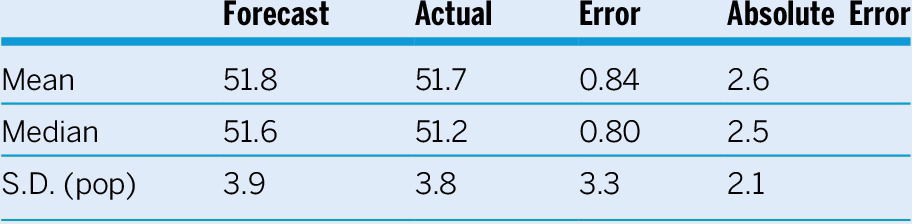
Table 1 displays the descriptive statistics—the mean, median, and standard deviation of the population, because the collection represents a universe, not a sample—of four variables: the forecasts, the actual incumbent share of the two-party vote (Leip Reference Leip2020), the arithmetic error, and the absolute error. Remarkably, the average ensemble forecast is within one percentage point of the actual. The mean (MAE) and median (MdAE) of the absolute error are within three percentage points of the actual, which is within range of the two-point error in the final preelection poll taken in late October or early November for the same elections;Footnote 4 this high level of accuracy was obtained even though most of the forecasts were issued months in advance of the election.
Forecasts of Incumbent Two-Party Vote, 1984–2016, Descriptive Statistics
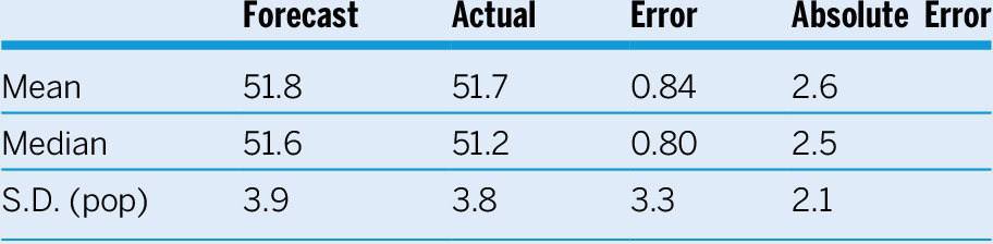
Note: N=13 forecasters, 63 forecasts.
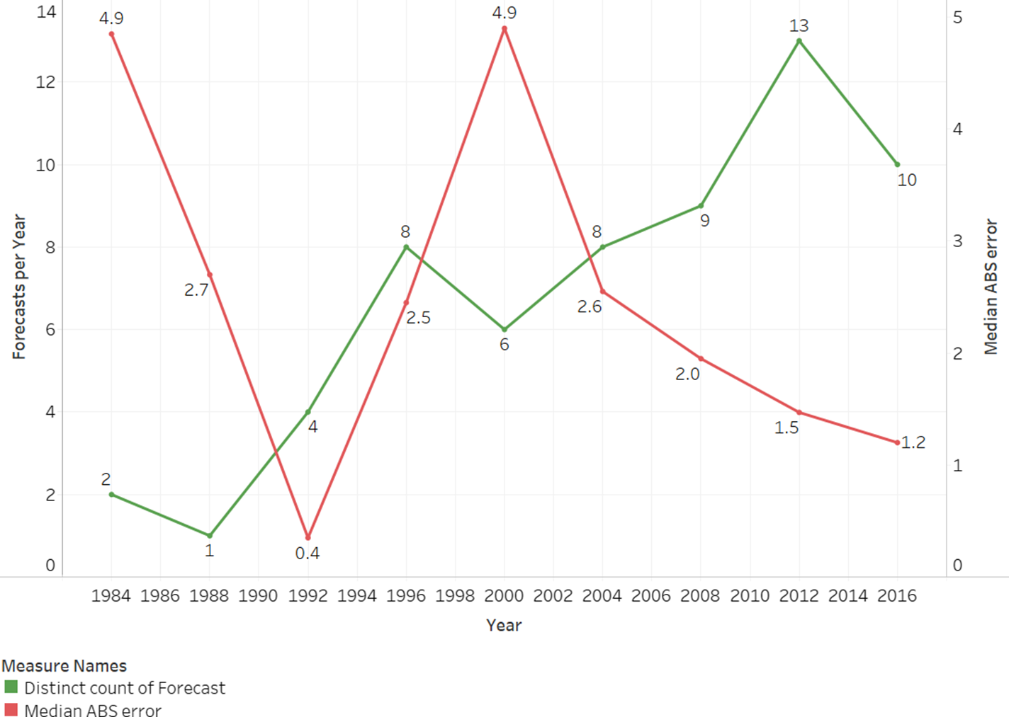
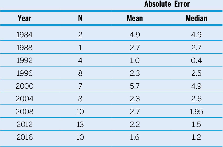
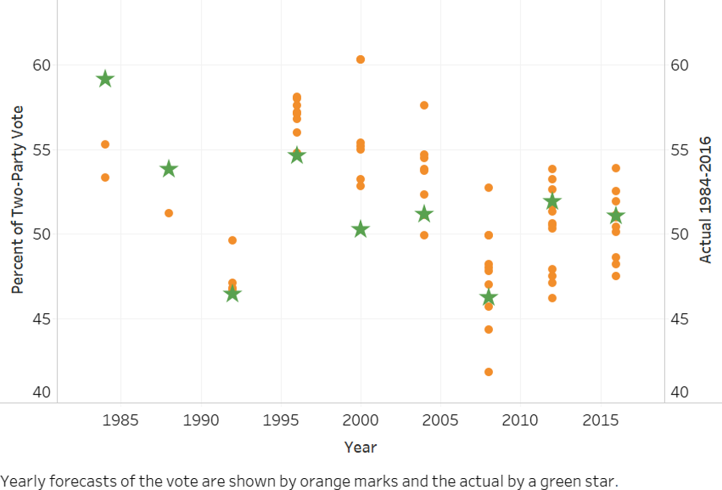
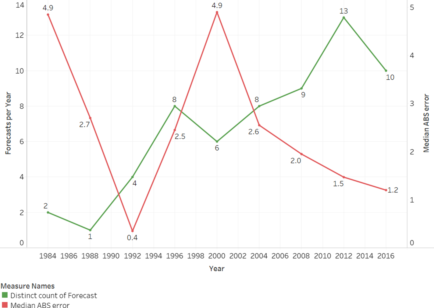
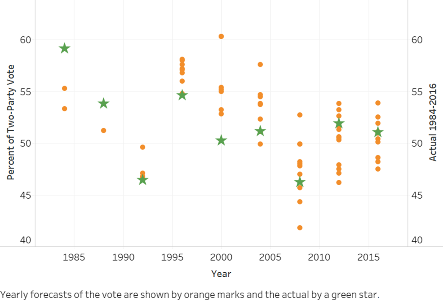
Figure 1 shows that, as the number of forecasts increased, the average error fell. Observe, in table 2, that the Pearson’s correlation coefficient measuring the relationship between the number of forecasts and the absolute error is weak over the entire period but strengthens substantially after the first three elections are dropped. Additionally, figure 2 reveals that the more recent forecasts bracket the actual value, which goes a long way in accounting for the greater accuracy of the ensemble forecasts. Thus, H1 receives empirical support: as the number of forecasts increased, they bracketed the actual value more frequently, making for greater accuracy.
Median Absolute Error by Number of Forecasts
Absolute Error by Number of Forecasts
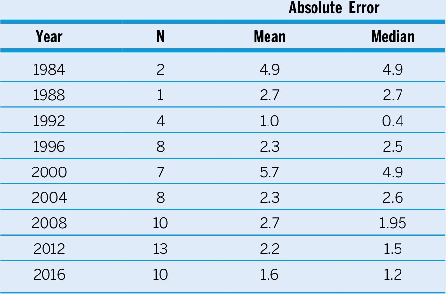
Note: Correlation coefficients: 1984–2016: r=-0.27 (MAE); r=-0.38 (MdAE) and 1996–2016: r=-0.54 (MAE); r=-0.74 (MdAE).
Incumbent Vote: Forecasts and Actual, by Year
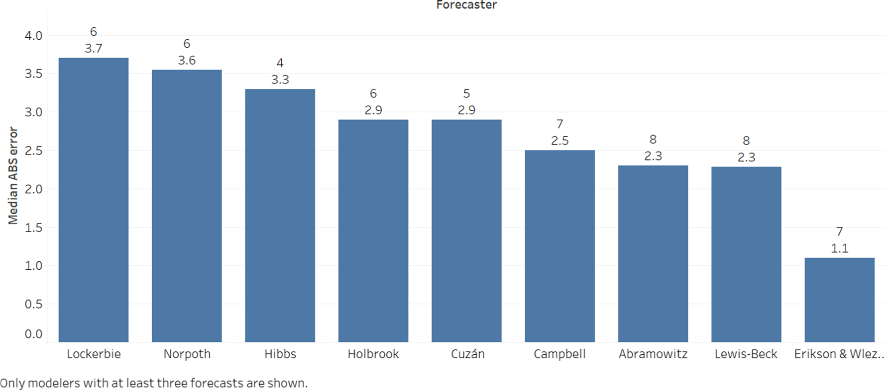
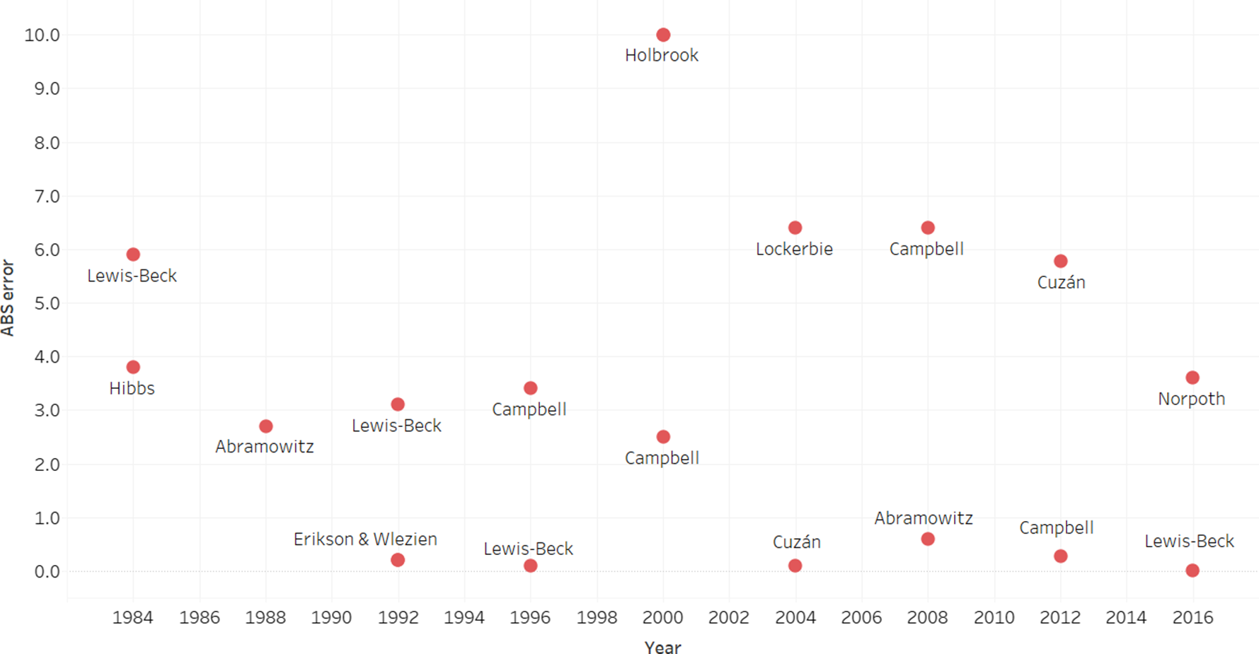
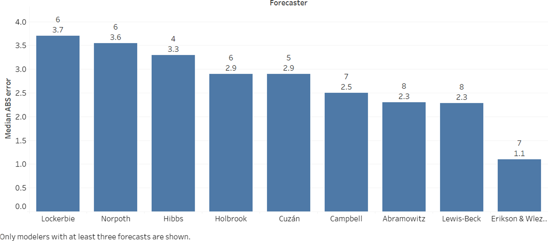
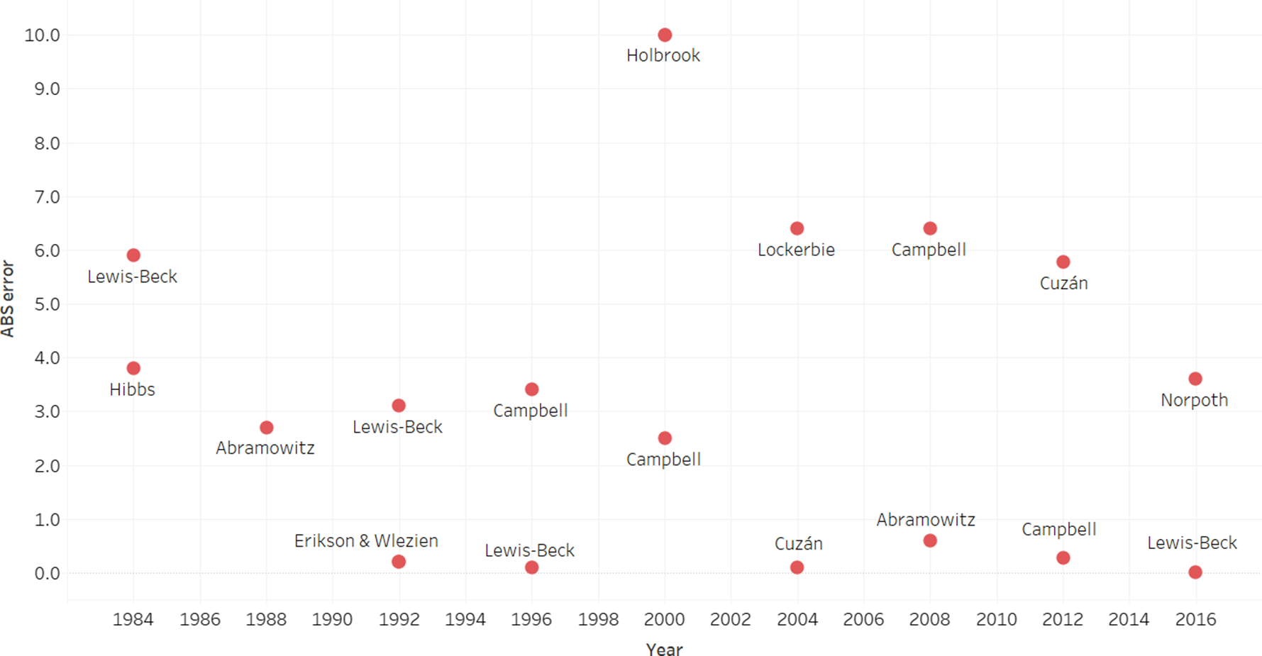
Turning to the modelers, figure 3 arranges the MdAE of their forecasts from left (highest) to right (lowest). The median is more applicable, because, with so few observations, outliers exert a distorting effect. The figure also shows the number of forecasts made by each member of the collection. Among those with at least five forecasts, Abramowitz, Campbell, Lewis-Beck, and Erikson and Wlezien have the best record for accuracy. However, as figure 4 demonstrates, this does not mean any one model comes closest to the actual year after year. In fact, in some cases the forecaster incurred the largest error only to win the gold an election or two later (e.g., Lewis-Beck 1992–96, Campbell 1996–2000)—or vice versa (Cuzán 2004–2012). Hypothesis 2, then, also finds support: no one modeler arrived first (or last) every time.
Median Absolute Error by Modeler and Number of Forecasts
Lowest and Largest Absolute Error, by Year
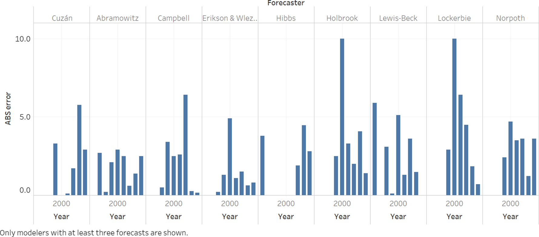
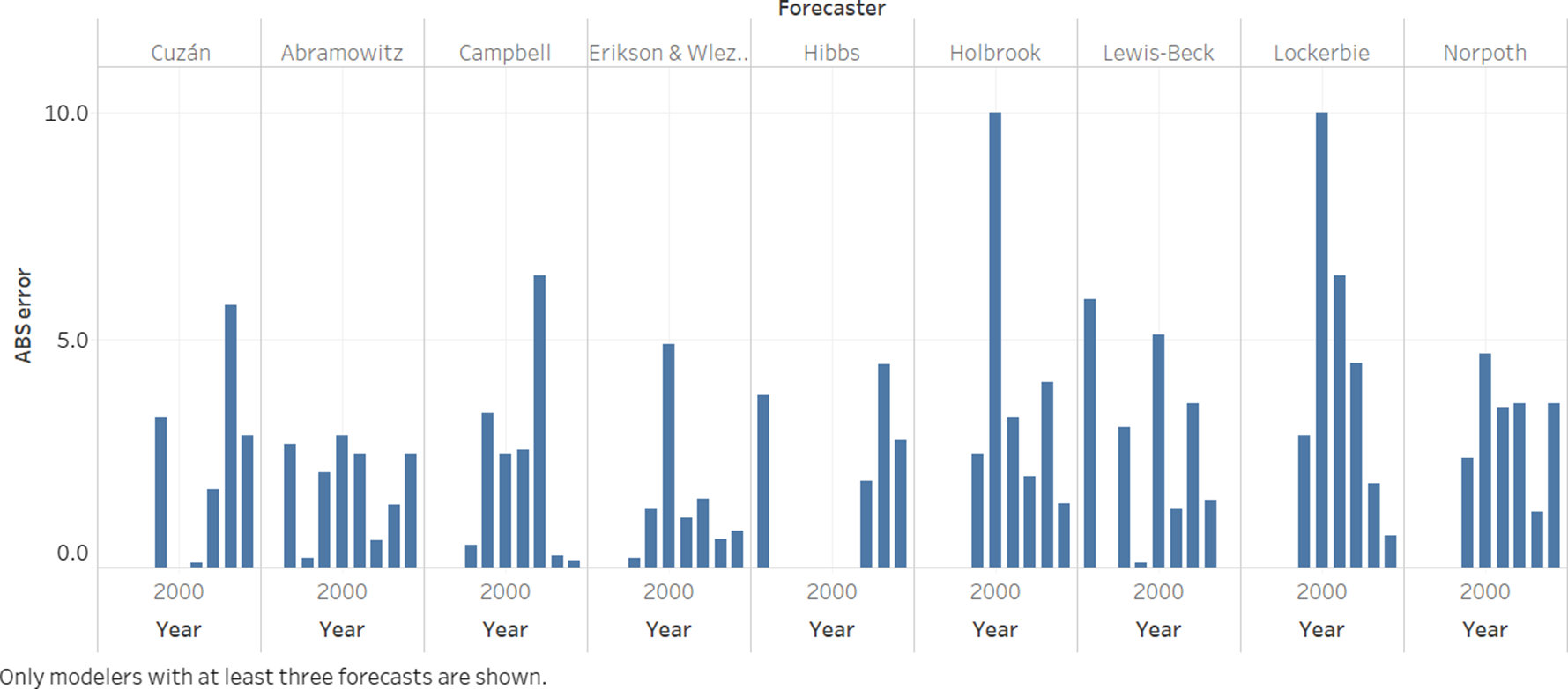
Finally, figure 5 displays the AE by forecaster by year. This allows us to determine whether any learning took place over time. It appears that this is the case with Holbrook, Lewis-Beck, and Lockerbie. In all three, following an early outlier the error progressively shrank and is now among the lowest. No other forecaster shows such improvement, although Campbell, and Erikson and Wlezien did recover nicely from the 2008 and 2000 outliers, respectively. In Cuzán’s case, however, the trend appears to go the other way.Footnote 5 For Abramowitz, Hibbs, and Norpoth, the error is trendless. Of course, in the case of Abramowitz, whose absolute error has consistently remained below 3.0, little learning was called for in the first place. Also, as Wink (Reference Wink2018–19, 206) points out, Abramowitz and Norpoth are the only ones who correctly called the winner in all three of the most recent elections. In any case, although outside the scope of this review, studying the changes that Holbrook, Lewis-Beck, and Lockerbie made in their models may well be instructive.
Forecaster Error by Year, 1992–2016
DISCUSSION AND CONCLUSION
As a group, the models in the Campbell Collection of Presidential Election Forecasts perform remarkably well over the 1984–2016 period. The aggregate may not do as well as other methods in any one election (Graefe et al., Reference Graefe, Armstrong, Jones and Cuzán2014), but across the entire period the record is impressive. Ironically, according to one study, the experts assembled in the quadrennial PollyVote Project appear to be more influenced by polls than by the models (Graefe Reference Graefe2018; see, also, Jones and Cuzán Reference Jones and Cuzán2013).
The foregoing analysis lends empirical support for both of the hypotheses set at the outset. As the Campbell Collection grew in numbers and diversity of inputs and methods, the ensemble forecast became more accurate; it did so because, with more models, it became more likely that at least two members of the group would bracket the actual value. Yet no one modeler turned out to be consistently the best performer across all elections. The lesson is that one should not place too much confidence in any one model but instead should look to the group mean or median forecast, a recommendation that is in keeping with the findings of the PollyVote Project.
As the Campbell Collection grew in numbers and diversity of inputs and methods, the ensemble forecast became more accurate; it did so because, with more models, it became more likely that at least two members of the group would bracket the actual value.
Peering into the future is always fraught with risk, but given these findings, and considering that the number and variety of models lined up in this symposium exceed that in all previous collections, there is one prediction I am willing to make. The error of the vote forecast will be, if not the lowest, among the lowest on record.
ACKNOWLEDGMENTS
I am grateful to the University of West Florida for the generous support and benign academic environment. For their comments and suggestions, I thank Randall J. Jones Jr. (who also found some of the early forecasts), Carl Klarner, Kyle Kondik, and Christopher Wlezien, as well as anonymous reviewers and the editors of this journal and of this symposium in particular. I am also appreciative of the work done on the PollyVote project in collaboration with J. Scott Armstrong, Randall J. Jones Jr., and Andreas Graefe. Finally, the usual disclaimer applies: all errors of fact or interpretation are my own.
SUPPLEMENTARY MATERIALS
To view supplementary material for this article, please visit http://dx.doi.org/10.1017/S1049096520001341.