


1. Introduction and results
1.1 Kinetically constrained models
Kinetically constrained models (KCM) are a class of interacting particle systems used since the 1980s to model the liquid-glass transition [Reference Fredrickson and Andersen12, Reference Fredrickson and Andersen13] (see [Reference Garrahan, Sollich and Toninelli14, Reference Ritort and Sollich31] for reviews). We will be interested in the very general class of
 $\,\mathcal{U}$
-KCM first introduced by Cancrini, Martinelli, Roberto and Toninelli in 2008 [Reference Cancrini, Martinelli, Roberto and Toninelli6], which includes all previously considered cases on
 ${{\mathbb{Z}}}^d$
.
Let us start by introducing these models directly on the two-dimensional lattice, to which we restrict our attention. A KCM is a Markov process with state space
 $\Omega=\{0,1\}^{{{\mathbb{Z}}}^2}$
. For a configuration
 $\eta\in\Omega$
and a site
 $x\in{{\mathbb{Z}}}^2$
, we denote
 $\eta_x$
the value of
 $\eta$
at x. We say that x is empty or infected if
 $\eta_x=0$
and that it is occupied or healthy if
 $\eta_x=1$
. We thus naturally identify a configuration
 $\eta\in\Omega$
with the set of its infected sites, so that
 $\eta\subset {{\mathbb{Z}}}^2$
.
A
 $\mathcal{U}$
-KCM is specified by two parameters—an update family
 $\mathcal{U}$
and an equilibrium measure
 $\mu$
. The measure
 $\mu$
on
 $\Omega$
is chosen to be the product Bernoulli measure such that each site is infected with probability
 $q>0$
and healthy with probability
 $1-q$
. All asymptotics hereafter are taken as
 $q\rightarrow0$
. The update family
 $\mathcal{U}$
is a finite set of finite nonempty subsets of
 ${{\mathbb{Z}}}^2\backslash \{0\}$
called update rules. The dynamics is the following. For each site
 $x\in{{\mathbb{Z}}}^2$
at rate 1 (i.e. at the times given by a Poisson point process on
 $\mathbb{R}_+$
with intensity 1) we attempt to update
 $\eta_x$
by replacing it by an independent Bernoulli
 $(1-q)$
variable. However, the update is only performed if there exists an update rule
 $U\in\mathcal{U}$
such that
 $\eta\supset (x+U)$
, while otherwise the configuration remains unchanged. In more formal terms the generator of the Markov process is the following for any function
 $f\,{:}\,\Omega\mapsto{{\mathbb{R}}}$
depending on a finite number of sites.
 \begin{equation*}\mathcal{L}(\,f)(\eta)=\sum_{x\in {{\mathbb{Z}}}^2}{{\mathbb{m}{1}}}_{\{\exists U\in\mathcal{U},\eta_{x+U}=0\}}(\mu_x(\,f)-f)(\eta),\end{equation*}
where
 $\eta_X$
denotes the restriction of
 $\eta$
to
 $X\cap{{\mathbb{Z}}}^2$
for
 $X\subset{{\mathbb{R}}}^2$
and
 $\mu_x(\,f)$
denotes the average of f with respect to
 $\eta_x$
conditionally on all other occupation variables. We further view
 $\eta_X$
as the element of
 $\{0,1\}^{{{\mathbb{Z}}}^2}$
equal to
 $\eta$
in
 $X\cap{{\mathbb{Z}}}^2$
and to 1 elsewhere. For background on the theoretical foundations of such interacting particle systems the reader is referred to [Reference Liggett24]. In particular,
 $\mu$
is indeed a reversible invariant measure for the
 $\mathcal{U}$
-KCM.
For any KCM arguably the most natural quantity of interest describing the speed at which memory of the initial state is lost is the first infection time of the origin
 \begin{equation*}\tau_0=\inf\{t\geqslant 0, (\eta(t))_0=0\}\in[0,\infty],\end{equation*}
where
 $(\eta(t))_{t \geqslant 0}$
denotes the
 $\mathcal{U}$
-KCM process. As we will concentrate on the equilibrium properties of the KCM, we will rather be concerned with
 ${{\mathbb{E}}}_\mu[\tau_0]$
, that is the expectation of
 $\tau_0$
with respect to the law of the stationary
 $\mathcal{U}$
-KCM with initial condition distributed according to its equilibrium measure
 $\mu$
.
1.2 Bootstrap percolation and universality
Bootstrap percolation is a close relative of KCM, though the two fields remained relatively independent for decades. Formally, the continuous time version of
 $\mathcal{U}$
-bootstrap percolation is the
 $\mathcal{U}$
-KCM with
 $q=1$
. However, bootstrap percolation has important additional properties and has attracted a great deal of attention with different motivation, also in non-lattice settings, as well as from computer science and sociological perspectives. We direct the reader to [Reference de Gregorio, Lawlor and Dawson9, Reference Morris30] and the references therein for an overview of this rich field.
In
 $\mathcal{U}$
-bootstrap percolation (the update family
 $\mathcal{U}$
being as above), for each integer
 $t \geqslant 0$
, a set
 $A_t$
of infected sites at time t is constructed as follows. Given an initial set of infected sites
 $A_0\subset {{\mathbb{Z}}}^2$
we set for all integers
 $t\geqslant 0$
 \begin{equation*}A_{t+1}=A_t\cup\{x\in{{\mathbb{Z}}}^2\,{:}\,\exists U\in\mathcal{U},x+U\subset A_t\}.\end{equation*}
That is, at each discrete time step the sites such that the translate of a rule by the corresponding site is already fully infected also become infected, while infections never heal. Thus, given the initial condition,
 $\mathcal{U}$
-bootstrap percolation is a monotone deterministic cellular automaton. For any set
 $A_0\subset {{\mathbb{Z}}}^2$
we denote by
 $[A_0]=\bigcup_{t\geqslant0}A_t$
its closure with respect to the
 $\mathcal{U}$
-bootstrap percolation process, that is the sites that are eventually infected when the initial infection is
 $A_0$
(we may also use this notation when
 $A_0 \not\subset{{\mathbb{Z}}}^2$
; it will then mean
 $[A_0 \cap {{\mathbb{Z}}}^2]$
). The best-studied setting, which is also the one relevant to us, is taking
 $A_0$
random with law
 $\mu$
, so that each site is infected independently with probability q. In this case the most prominent questions are for which values of q we have
 $[A_0]={{\mathbb{Z}}}^2$
a.s. and, for such values of q, what is the typical order of magnitude of the infection time of the origin
 $\tau_0$
defined as for KCM.
The general
 $\mathcal{U}$
-bootstrap percolation framework only gained visibility after the work of Bollobás et al. [Reference Bollobás, Smith and Uzzell5]. They introduced several crucial notions, which we discuss next. We invite the reader unfamiliar with these notions to systematically consult the examples in Figure 1 and apply the definitions to them.
We denote by
 $S^1=\{z\in{{\mathbb{R}}}^2,\|z\|=1\}$
the unit circle, which we standardly identify with
 ${{\mathbb{R}}}/2\pi{{\mathbb{Z}}}$
, where
 $\|\!\cdot\!\|$
is the Euclidean norm of
 ${{\mathbb{R}}}^2$
(all distances in this work will be Euclidean, denoted by
 $d(\cdot,\cdot)$
). A direction
 $u \in S^1$
will be called rational when
 $\tan u \in {{\mathbb{Q}}} \cup \{\infty\}$
. For a direction
 $u\in S^1$
and a scalar
 $x\in{{\mathbb{R}}}$
, we define the open half-plane
 ${{\mathbb{H}}}_u(x)=\{y\in{{\mathbb{R}}}^2,\langle u,y\rangle<x\}$
directed by u translated by x, and
 $\bar {{\mathbb{H}}}_u(x)=\{y\in{{\mathbb{R}}}^2,\langle u,y\rangle\leqslant x\}$
the corresponding closed half-plane. We further set
 ${{\mathbb{H}}}_u={{\mathbb{H}}}_u(0)$
. A direction
 $u\in S^1$
is said to be unstable (for
 $\mathcal{U}$
) if there exists
 $U\in\mathcal{U}$
such that
 $U\subset {{\mathbb{H}}}_u$
and stable otherwise. It is not hard to see (Theorem 1.10 of [Reference Bollobás, Smith and Uzzell5], Lemma 2.6 of [Reference Bollobás, Duminil-Copin, Morris and Smith4]) that the set of stable directions is a finite union of closed intervals of
 $S^1$
with rational endpoints. Bollobás et al. [Reference Bollobás, Smith and Uzzell5] introduced the following partition of update families into three classes. In order to state their results and others, we will need the following standard asymptotic notation. For any real functions f(q), g(q) defined for
 $q>0$
sufficiently small, with
 $g>0$
, we write
-
•
 $f(q)=\Theta(g(q))$
when
$c g(q) \leqslant f(q) \leqslant C g(q)$
,
-
•
$f(q)=\Omega(g(q))$
when
$f(q) \geqslant c g(q)$
, -
•
$f(q)=O(g(q))$
when
$|\,f(q)| \leqslant Cg(q)$


for some constants
 $0 < c \leqslant C < +\infty$
when
 $q>0$
is sufficiently small. Finally, we write
 $f(q)=o(g(q))$
when
 $\frac{|\,f(q)|}{g(q)} \rightarrow 0$
when
 $q \rightarrow 0$
. Let us note that all such implicit constants are allowed to depend on the update family
 $\mathcal{U}$
and all (finite sets of) directions considered, but never on q.
Definition 1.1 (Definition 1.3 of [Reference Bollobás, Smith and Uzzell5]) An update family
 $\mathcal{U}$
is called
-
• supercritical if there exists an open semicircle of unstable directions,
-
• critical if it is not supercritical, but there exists an open semicircle with a finite number of stable directions,
-
• subcritical otherwise.
In [Reference Bollobás, Smith and Uzzell5] it was proved that for supercritical models
 $\tau_0=q^{-\Theta(1)}$
with high probabilityFootnote 1 as
 $q\rightarrow0$
, while for critical ones
 $\tau_0=\exp(q^{-\Theta(1)})$
. Completing the justification of Definition 1.1, Balister et al. [Reference Balister, Bollobás, Przykucki and Smith2] proved that for subcritical models
 $\tau_0=\infty$
with positive probability for q small enough. Albeit very general, these results were much less precise than what was known for most specific models studied previously, so one may view them as only qualitatively identifying the three different possible behaviours.
Supercritical models are fairly simple from the bootstrap percolation point of view, while still very little is known in general about subcritical ones [Reference Hartarsky16]. The remaining critical models are the most pursued. Bollobás, Duminil-Copin, Morris and Smith [Reference Bollobás, Duminil-Copin, Morris and Smith4] established much more precise quantitative results for this class. To state their results, we need some more notation.
Definition 1.2 (Definition 1.2 of [Reference Bollobás, Duminil-Copin, Morris and Smith4]) Let
 $\mathcal{U}$
be a critical update family and
 $u\in S^1$
be a direction. Then the difficulty of
 $u,\alpha(u)$
, is defined as follows.
-
• If u is unstable, then
$\alpha(u)=0$
. -
• If u is an isolated stable direction (isolated in the topological sense), then
that is the minimal number of additional infections allowing
\begin{equation*} \alpha(u)=\min\{n\in[1,\infty) \,{:}\, \exists\ Z\subset{{\mathbb{Z}}}^2,|Z|=n,|[{{\mathbb{H}}}_u\cup Z]\backslash {{\mathbb{H}}}_u|=\infty\},\end{equation*}
${{\mathbb{H}}}_u$
to infect an infinite set of sites.Footnote 2
-
• Otherwise,
$\alpha(u)=\infty$
.


We define the difficulty of
 $\mathcal{U}$
by
 \begin{equation}\alpha(\mathcal{U})=\min_{C\in\mathcal{C}}\max_{u\in C}\alpha(u)\in[1,\infty),\end{equation}
where
 $\mathcal{C}=\{{{\mathbb{H}}}_u\cap S^1 \,{:}\, u\in S^1\}$
is the set of open semicircles of
 $S^1$
.
Definition 1.3 (Definition 1.3 of [Reference Bollobás, Duminil-Copin, Morris and Smith4]) A critical update family with difficulty
 $\alpha$
is balanced if there exists a closed semicircle in which all directions have difficulty at most
 $\alpha$
and is unbalanced otherwise.
With these definitions, the main result of Bollobás et al. [Reference Bollobás, Duminil-Copin, Morris and Smith4, Theorem 1.5], states
 \begin{equation}\tau_0=\begin{cases} \exp\left(\dfrac{\Theta(1)}{q^{\alpha(\mathcal{U})}}\right)&\text{for critical balanced models,}\\ \\[-7pt] \exp\left(\dfrac{\Theta((\log q)^2)}{q^{\alpha(\mathcal{U})}}\right)&\text{for critical unbalanced models}\end{cases}\end{equation}
with high probability as
 $q\rightarrow0$
. These are the best general estimates currently known, though for some specific choices of
 $\mathcal{U}$
sharper results are available [Reference Bollobás, Duminil-Copin, Morris and Smith3, Reference Duminil-Copin and van Enter10, Reference Gravner and Holroyd15, Reference Hartarsky and Morris22, Reference Holroyd23].
1.3 Universality for KCM
Supercritical KCM As we shall see, the situation for
 $\mathcal{U}$
-KCM is far more complex. Some new features already appear for supercritical models. The general setting was treated only recently by Martinelli et al. [Reference Martinelli, Morris and Toninelli27] and Martinelli, Toninelli and the second author [Reference Marêché, Martinelli and Toninelli26], who identified the two relevant classes of models.
Definition 1.4 (Definition 2.11 of [Reference Martinelli, Morris and Toninelli27]) A supercritical update family
 $\mathcal{U}$
is rooted if there exist two non-opposite stable directions and unrooted otherwise.
In [Reference Martinelli, Morris and Toninelli27] the upper bounds in the following result for
 $\mathcal{U}$
-KCM were established: as
 $q \rightarrow 0$
,
 \begin{equation}{{\mathbb{E}}}_\mu[\tau_0]=\begin{cases} \exp\left(\Theta(\log (1/q))\right)&\text{supercritical unrooted,}\\ \\[-7pt] \exp\left(\Theta((\log (1/q))^2)\right)&\text{supercritical rooted},\end{cases}\end{equation}
while the lower ones were supplied in [Reference Marêché, Martinelli and Toninelli26], the lower bound for unrooted models being trivial. The lower bound for rooted models relied mostly on a combinatorial result by the second author [Reference Marêché25] roughly stating that in order to infect the origin starting from a configuration in which the infection closest to the origin is at distance d from it, the dynamics has to go through a configuration with at least
 $\log d$
infections at distance at most d from the origin. This combinatorial bottleneck was originally identified in [Reference Sollich and Evans32] (see also [Reference Chung, Diaconis and Graham8]) for the archetypal one-dimensional supercritical rooted model, which is, perhaps, the simplest and best-studied KCM—the East model (see [Reference Faggionato, Martinelli, Roberto and Toninelli11] for a review). Extending the one-dimensional result to higher dimensions in [Reference Marêché25] required the development of a new approach, which will be the starting point for our analysis, although we will not be able to apply the result of [Reference Marêché25] itself.
Critical KCM Turning to critical models, a first observation is that bootstrap percolation provides an automatic lower bound for
 ${{\mathbb{E}}}_\mu[\tau_0]$
in the
 $\mathcal{U}$
-KCM with the same update family. In particular, it is easy to show (see [Reference Martinelli and Toninelli28, Lemma 4.3] and its improved version from [Reference Hartarsky, Martinelli and Toninelli20, Section 2]) that the expressions in (2) are lower bounds for
 ${{\mathbb{E}}}_\mu[\tau_0]$
for the corresponding
 $\mathcal{U}$
-KCM.
Led by the intuition from the results for supercritical models, Morris [Reference Morris29], presenting his work with Martinelli and Toninelli, introduced the following notion (we simplify his terminology slightly).
Definition 1.5 (Definition 2.3 of [Reference Morris29]) A critical update family of difficulty
 $\alpha$
is called rooted if there exist two non-opposite directions of difficulty strictly larger than
 $\alpha$
and unrooted otherwise.
Initially it was believed, as explained in [Reference Morris29], that if a critical model is unrooted, it satisfies
 ${{\mathbb{E}}}_\mu[\tau_0]=\exp(q^{-\alpha(\mathcal{U})+o(1)})$
as
 $q \rightarrow 0$
, but not if it is rooted. This conjecture was made more precise by the same authors in [Reference Martinelli, Morris and Toninelli27], who then suggested a different definition of rooted/unrooted reflecting the upper bounds they proved and conjectured to be tight.
However, both conjectures were disproved by Martinelli, Toninelli and the first author [Reference Hartarsky, Martinelli and Toninelli21], who proved stronger upper bounds than the ones in [Reference Martinelli, Morris and Toninelli27], in particular refuting the above conjectures for some rooted models and showing that the automatic bootstrap percolation lower bound is essentially sharp for them as well. In a parallel work Toninelli and the present authors [Reference Hartarsky, Marêché and Toninelli19] proved for all other models lower bounds essentially matching the upper ones from [Reference Martinelli, Morris and Toninelli27]. Hence, the combined results of [Reference Hartarsky, Marêché and Toninelli19, Reference Hartarsky, Martinelli and Toninelli21, Reference Martinelli, Morris and Toninelli27] proved the following universality picture featuring yet a different partition of critical models. As
 $q \rightarrow 0$
,
 \begin{equation*}{{\mathbb{E}}}_\mu[\tau_0]=\begin{cases} \exp\left(\dfrac{(\log(1/q))^{O(1)}}{q^{\alpha(\mathcal{U})}}\right)&\text{critical, finitely many stable directions,}\\ \\[-9pt] \exp\left(\dfrac{(\log(1/q))^{O(1)}}{q^{2\alpha(\mathcal{U})}}\right)&\text{critical, infinitely many stable directions}.\end{cases}\end{equation*}
This result shows that each universality class in bootstrap percolation (models with the same value of
 $\alpha(\mathcal{U})$
) splits into two universality classes of KCM. This should indeed be viewed as the critical counterpart of (3). While the lower bound of [Reference Hartarsky, Marêché and Toninelli19] establishing the result for models with infinitely many stable directions does reflect (and actually uses) the combinatorial bottleneck of the one-dimensional supercritical rooted East model, the upper bound of [Reference Hartarsky, Martinelli and Toninelli21] is based on a very peculiar efficient mechanism that uses a ‘quasi-local’ East-type movement resulting in a supercritical unrooted dynamics on larger length scales. However, it remained unclear whether this fairly unnatural mechanism of [Reference Hartarsky, Martinelli and Toninelli21] and the purely East-like one used in [Reference Martinelli, Morris and Toninelli27] are indeed the correct ones for all models concerned.
1.4 Results
Our goal is to identify the dominant relaxation mechanisms for each model, which are reflected in the scaling of
 $\tau_0$
. Therefore, together with the companion work by the first author [Reference Hartarsky17], we determine
 $\log{{\mathbb{E}}}_\mu[\tau_0]$
up to a constant factor. In the present paper we establish all lower bounds by identifying the correct bottleneck (see Section 2), while the companion one [Reference Hartarsky17] provides the remaining matching upper bounds by exhibiting efficient relaxation mechanisms for all critical
 $\mathcal{U}$
-KCM.
In order to state our results we introduce the last bit of notation needed to define the seven refined universality classes of critical
 $\mathcal{U}$
-KCM, which we identify.
Definition 1.6 A critical update family of difficulty
 $\alpha$
is called
-
• isotropic if there is no direction of difficulty strictly greater than
$\alpha$
, -
• semi-directed if there exists exactly one direction of difficulty strictly greater than
$\alpha$
.


Notice that the isotropic/semi-directed critical models form a partition of unrooted balanced critical ones.
Theorem 1.7 Let
 $\mathcal{U}$
be a critical update family with difficulty
 $\alpha$
and infinite number of stable directions. We have the following alternatives as
 $q\rightarrow0$
.
-
(a) If
$\,\mathcal{U}$
is unbalanced, that is there exist two opposite directions
$u\in S^1$
with
$\alpha(u)>\alpha$
, then
\begin{equation*}{{\mathbb{E}}}_\mu[\tau_0]=\exp\left(\frac{\Theta\left(\left(\log (1/q)\right)^4\right)}{q^{2\alpha}}\right)\!.\end{equation*}
-
(b) If
$\,\mathcal{U}$
is balanced, that is there do not exist two opposite directions
$u\in S^1$
with
$\alpha(u)>\alpha$
, then
\begin{align*}\\[-25pt]{{\mathbb{E}}}_\mu[\tau_0]=\exp\left(\frac{\Theta(1)}{q^{2\alpha}}\right)\!.\end{align*}


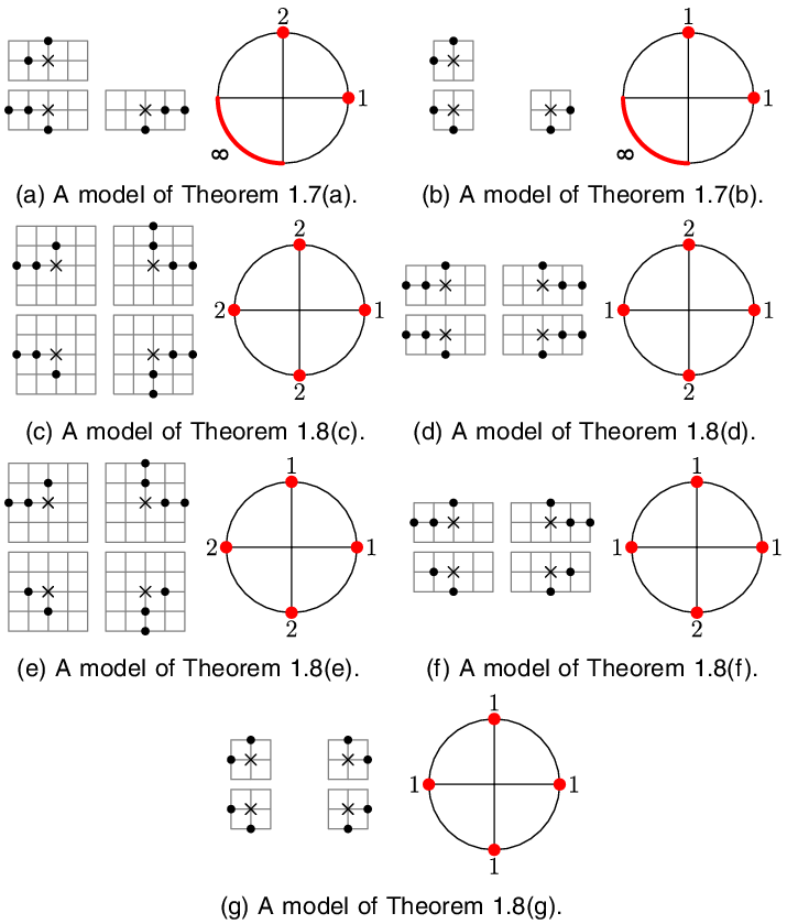
Representative models of each of the seven refined universality classes of critical
 $\,\mathcal{U}$
-KCM. For each one the update rules are depicted on the left with 0 marked by a cross and the sites of the rule denoted by dots. The figure on the right gives the stable directions, which are thickened and have their difficulties next to them. The isolated stable directions are marked by dots. In all cases the difficulty
 $\alpha$
of the model is 1, as witnessed by the right-hand open semicircle.

The upper bounds are proved in [Reference Martinelli, Morris and Toninelli27, Theorem 2(a)] and [Reference Hartarsky17, Theorem 1(b)] respectively. Furthermore, for one specific model of the class (a), the Duarte model, this result was known from [Reference Marêché, Martinelli and Toninelli26]. A different proof of the lower bound for case (b) was given in [Reference Hartarsky, Marêché and Toninelli19].
Theorem 1.8 Let
 $\mathcal{U}$
be a critical update family with difficulty
 $\alpha$
and finite number of stable directions. We have the following alternatives as
 $q\rightarrow0$
.
-
(c) If
$\,\mathcal{U}$
is unbalanced rooted, that is there exist at least three directions
$u\in S^1$
with
$\alpha(u)>\alpha$
, two of which are opposite, then
\begin{equation*}{{\mathbb{E}}}_\mu[\tau_0]=\exp\Bigg(\frac{\Theta\left(\left(\log (1/q)\right)^3\right)}{q^{\alpha}}\Bigg).\end{equation*}
-
(d) If
$\,\mathcal{U}$
is unbalanced unrooted, that is there exist exactly two directions
$u\in S^1$
such that
$\alpha(u)>\alpha$
and they are opposite, then
\begin{equation*}{{\mathbb{E}}}_\mu[\tau_0]=\exp\left(\frac{\Theta\left(\left(\log(1/q)\right)^2\right)}{q^{\alpha}}\right)\!.\end{equation*}
-
(e) If
$\,\mathcal{U}$
is balanced rooted, that is there exist at least two directions
$u\in S^1$
with
$\alpha(u)>\alpha$
, but not two opposite ones, then
\begin{equation*}{{\mathbb{E}}}_\mu[\tau_0]=\exp\left(\frac{\Theta\left(\log (1/q)\right)}{q^{\alpha}}\right)\!.\end{equation*}
-
(f) If
$\,\mathcal{U}$
is semi-directed, that is there exists exactly one direction
$u\in S^1$
such that
$\alpha(u)>\alpha$
, then
\begin{equation*}{{\mathbb{E}}}_\mu[\tau_0]=\exp\left(\frac{\Theta\left(\log\log (1/q)\right)}{q^{\alpha}}\right)\!.\end{equation*}
-
(g) If
$\,\mathcal{U}$
is isotropic, that is there exists no direction
$u\in S^1$
such that
$\alpha(u)>\alpha$
, then
\begin{equation*}{{\mathbb{E}}}_\mu[\tau_0]=\exp\left(\frac{\Theta(1)}{q^{\alpha}}\right)\!.\end{equation*}


The upper bound in (c) was proved in [Reference Hartarsky, Martinelli and Toninelli21, Theorem 1], while the remaining upper bounds are from [Reference Hartarsky17, Theorem 1]. The lower bounds for cases (d) and (g) follow automatically from bootstrap percolation results and [Reference Martinelli and Toninelli28, Lemma 4.3] as discussed in the previous section.
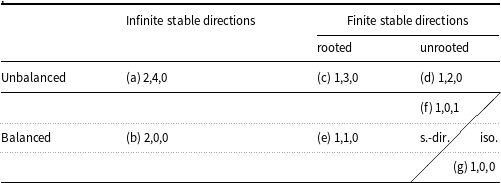
The classification results, assuming the remaining matching bounds of [Reference Hartarsky17], are summarised in Table 1. In addition, a simple representative of each class is given in Figure 1 for the reader’s convenience.
Classification of critical
 $\mathcal{U}$
-KCM with difficulty
 $\alpha$
. Assuming [Reference Hartarsky17], for each class
 ${{\mathbb{E}}}_\mu[\tau_0]=\exp\big(\Theta(1)\big(\frac{1}{q^\alpha}\big)^{\beta}\left(\log \frac{1}{q}\right)^\gamma \big(\log\log\frac{1}{q}\big)^\delta\big)$
as
 $q \rightarrow 0$
. The label of the class and the exponents
 $\beta,\gamma,\delta$
are indicated in that order

Remark 1.9 The lower bounds we prove in Theorems 1.7 and 1.8 for
 ${{\mathbb{E}}}_\mu[\tau_0]$
also hold for another important characteristic timescale of the corresponding
 $\mathcal{U}$
-KCM, the relaxation time
 ${T_{\textrm{rel}}}$
(see e.g. [Reference Hartarsky, Marêché and Toninelli19, Definition 2.5]), which is another measure of the speed at which the memory of the initial state is lost. Indeed, [Reference Martinelli, Morris and Toninelli27, Equation (2.8)] yields
 ${T_{\textrm{rel}}} \geqslant q{{\mathbb{E}}}_\mu[\tau_0]$
.
1.5 Comments
Let us emphasise that, contrary to what is the case in bootstrap percolation, where the exact asymptotics and corrective terms of
 $\log \tau_0$
are sometimes known, for KCM there exists only one model (the Duarte model treated by Martinelli, Toninelli and the second author [Reference Marêché, Martinelli and Toninelli26]) for which
 $\log{{\mathbb{E}}}_\mu[\tau_0]$
is determined up to a constant factor and none for which the exact asymptotics is known. Thereby, the combined results of [Reference Hartarsky17, Reference Hartarsky, Martinelli and Toninelli21, Reference Martinelli, Morris and Toninelli27] and the present work improve the best known results for all critical
 $\mathcal{U}$
-KCM except the Duarte-KCM and give a new proof of the best known results for that last model. In view of the state of the art in the simpler setting of
 $\mathcal{U}$
-bootstrap percolation, it does not seem currently feasible to pursue higher precision in full generality for critical
 $\mathcal{U}$
-KCM. Theorem 1.7 establishes the lower bounds of [Reference Hartarsky, Marêché and Toninelli19, Conjecture 7.1], while Theorem 1.8 proves the ones of [Reference Hartarsky, Martinelli and Toninelli21, Conjecture 6.1] (that conjecture was intentionally not as precise concerning the semi-directed case (f), which seemed quite mysterious at the time of writing of the conjecture).
What is more, the present work treats all lower bounds in a systematic and comprehensive way, by showing that the main obstacle for the dynamics in all cases corresponds to a combinatorial bottleneck similar to the one of the two-dimensional East model (see Section 2 for more details). Moreover, the core of our argument carries over to higher dimensions with no further difficulty, thus reducing such lower bounds for higher-dimensional KCM to estimates for their bootstrap percolation counterparts.
1.6 Organisation of the paper
The remainder of the paper is organised as follows. In Section 2 we provide an outline of the ideas of the proof. The core of the proof is Section 3, where we establish the general combinatorial bottleneck for KCM dynamics. In Section 4 we deduce our main results, Theorems 1.7 and 1.8, very directly from Proposition 3.7. It is not until Section 4 that the distinction between the different classes of models becomes relevant. In addition to the central Proposition 3.7, Section 4 requires several estimates regarding bootstrap percolation. These estimates are established in the appendices of the arXiv version of this paper [Reference Hartarsky and Marêché18], which are not included here as they are complex and contain few new ideas. Appendix A is rather standard and provides bounds on the probability of ‘spanning’ by uniting arguments of Bollobás et al. [Reference Bollobás, Duminil-Copin, Morris and Smith4] and of Toninelli and the authors [Reference Hartarsky, Marêché and Toninelli19] without significant new input. This appendix may still be of interest to bootstrap percolation specialists, as it gives a simplification of the most technical part of the proof of the main result of [Reference Bollobás, Duminil-Copin, Morris and Smith4]. In Appendix B we establish bounds on the probability of a notion of ‘crossing’ inspired from [Reference Bollobás, Duminil-Copin, Morris and Smith4] but modified to suit our setting (see Section 2), which are not particularly difficult given Appendix A.
2. Outline of the proof
Let us outline the main highlights of the proof, emphasising new ideas with respect to our main sources of inspiration [Reference Bollobás, Duminil-Copin, Morris and Smith4, Reference Hartarsky17, Reference Hartarsky, Marêché and Toninelli19, Reference Marêché25]. The differences between the various universality classes will be much more apparent in [Reference Hartarsky17], where efficient mechanisms for the infection of the origin are implemented for each class. Since one of the main virtues of our work is that the core argument is independent of the universality class, we invite the reader willing to understand the origin of the choices of length scales appearing in Section 4 to consult [Reference Hartarsky17], which is also our inspiration for choosing them. For the sake of concreteness, unless otherwise indicated, in this section we restrict our attention to the representative of the class (e) of rooted balanced models with finitely many stable directions given in Figure 1e.
The proof relies on the notion of ‘bottleneck’: we show that before the origin can be infected, the dynamics has to go through a set of configurations with a probability small enough so that this does not happen for a very long time.
Morally speaking, in this model the smallest mobile entity (‘droplet’) is an infected square of size roughly
 $1/q$
. Indeed, typically on its right and top sides one can find an infection, which allows it to infect the column of sites on its right and the row of sites above it. However, it is essentially impossible for the infection to grow down or left, as this requires two consecutive infections and those are typically only available at distance
 $1/q^2$
from the droplet. We will only work in a region R of size
 $1/q^{7/4}$
around the droplet, so, morally, such couples of infections are not available. Thus, we can think of the droplet as performing the following simpler dynamics. If there is a droplet present at a certain position, it may create/destroy another one above it and to its right. Therefore, the droplets follow the dynamics of the two-dimensional supercritical rooted KCM called East model.
As mentioned in the introduction, for supercritical rooted models, including the (two-dimensional) East one, the second author established in [Reference Marêché25] the following bottleneck: in order for an infection (representing a droplet in our original model) to reach the centre of a box R of size
 $3^{n}$
initially fully healthy it is necessary to visit a configuration with at least n infections simultaneously present in the box. This was achieved by an inductive argument that we describe next. It is enough to show that if R is initially fully healthy and we can only have strictly less than n infections at the same time in R, we cannot reach a configuration with all infections in the middle of R. Indeed, this implies that there are strictly less than
 $n-1$
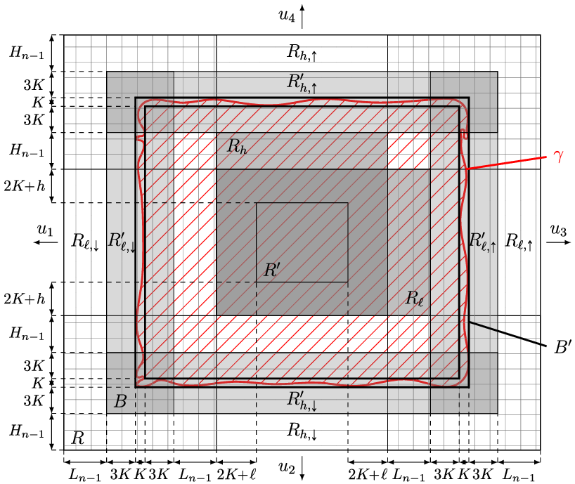
infections at the same time in the middle of R, and one can make an induction on n. To show that we cannot reach a configuration with all infections in the middle of R, by reversibility we may instead prove that if we start with infections only in the middle of R, but we are never allowed to have n infections simultaneously in R, we cannot reach a configuration fully healthy in R. The idea is to ensure that for any path of the dynamics starting with all infections in the middle of R in which we never have n infections at the same time in R, the following two conditions remain true at all times. Firstly, a buffer zone (see the shaded frame B in Figure 2) with no infections remains intact. Secondly, there is always an infection in the internal region encircled by the buffer, so the dynamics cannot reach a configuration completely healthy in R.
In order to achieve that, we use a second induction, on the step of the path. We know that so far an infection remains trapped in the internal region encircled by the buffer, so we only have
 $n-1$
infections available for disrupting the buffer from the outside, which is impossible by induction on n. Therefore, it suffices to show that we may not disrupt the buffer from the inside either. By projecting the two-dimensional East model on each axis it is clear that no infection can enter the left and bottom parts of the buffer from the inside, and the projections of the lowest and leftmost particles in the region inside the buffer need to remain where they were initially. The right part of the buffer (and similarly the top one) cannot be reached from the inside, because at least one infection needs to remain as far left as the leftmost initial one was, so we only have
 $n-1$
infections with which to reach the right part of the buffer, which is impossible by induction on n.
On a very high level we will proceed in the same way for critical models. However, there are several obvious problems in making the above reasoning rigorous for these models (in fact we do not think that a direct mapping to the two-dimensional East model can be made rigorous for our purposes). Firstly, we said above that the smallest mobile entities, ‘droplets,’ were infected squares of size
 $1/q$
, but the smallest mobile entities are actually more complicated. One needs to identify an event, which says whether or not something is a droplet and this event should be both deterministically necessary for infection to spread and sufficiently unlikely, so that having many droplets at the same time has probability small enough to be a good bottleneck. It turns out that the notion of ‘spanning’ introduced in [Reference Bollobás, Duminil-Copin, Morris and Smith4], following [Reference Cerf and Cirillo7] is flexible enough for us. Roughly speaking (see Definition 3.1), a droplet is spanned if the infections present inside it are sufficient to infect a connected set touching all its sides. We call a droplet critical if it has size roughly
 $1/q$
. It is known from [Reference Bollobás, Duminil-Copin, Morris and Smith4] and obtained again in the Appendix A of the arXiv version of this paper [Reference Hartarsky and Marêché18] in a more adapted form that the probability of a specific critical droplet being spanned is roughly
 $\exp(\!-1/q)$
. Unfortunately, given a configuration, spanned critical droplets may overlap, so in order to obtain good bounds on the probability of the configuration, one needs to consider disjointly occurring ones. We may then define the number of spanned critical droplets as the maximal number of disjointly occurring ones.
Having fixed these notions, we encounter a more significant issue—the (spanned critical) droplets may move a bit without creating another droplet, by changing their internal structure. Worse yet, they are not really forbidden to move left or down, but simply are not likely to be able to do so wherever they want: it depends on the dynamic environment. Indeed, being able to move by a single step down is allowed by the presence of a couple of infections on the side of the droplet, which has probability only as small as q and is by far not something we can ensure never happens up to time
 $T=\exp(\log (1/q)/q)$
.
In order to handle these problems we introduce the crucial notion of crossing (not to be confused, e.g. with the one of [Reference Bollobás, Duminil-Copin, Morris and Smith4]). Consider a vertical strip S of width
 $1/q^{3/2}$
of our domain, R, which is a square of size
 $1/q^{7/4}$
. Roughly speaking (see Definition 3.5 for a more precise statement), we say that S has a crossing if the following two events occur. Firstly, the infections in S together with the entire half-plane to the right of S are enough to infect a path from right to left in S (this is essentially the notion of crossing in [Reference Bollobás, Duminil-Copin, Morris and Smith4]). Secondly, S does not contain a spanned critical droplet. Notice that these two events go opposite ways—the former is favoured by infections, while the latter is not. In the Appendix B of the arXiv version of this paper [Reference Hartarsky and Marêché18], we show that the probability of a crossing decays exponentially with the width of S at our scales.
Having established such a bound on the probability of crossings, we may safely assume (it happens with high probability) that they never occur until time T and this is the property we use to formalise the intuition that ‘moving down or left is impossible.’ More precisely, assume that initially the only critical droplet is on the right of S and S never has a crossing. Then, simply because the KCM dynamics can never infect more than what bootstrap percolation can, starting from the same initial condition, the droplet will not be able to reach the left side of S. Indeed, if it could, there would be a ‘trail’ of infectable sites from the right of S to its left, which would imply a crossing.
3. Supercritical rooted dynamics of droplets
3.1 Setting and preliminaries
Let
 $\mathcal{U}$
be an update family. Assuming they exist, we further fix two non-collinear rational stable directions
 $u_1$
and
 $u_2$
. We set
 $u_3=u_1+\pi$
,
 $u_4=u_2+\pi$
and
 $\mathcal{T}=\{u_1,u_2,u_3,u_4\}$
. We will simply call parallelogram a set of the form
 \begin{align*}R(a,b;\ c,d)&=\left\{x\in{{\mathbb{R}}}^2\,|\,\langle x,u_3\rangle\in[a,c],\langle x,u_4\rangle\in[b,d]\right\}\\[3pt] &=\bar{{\mathbb{H}}}_{u_1}(\!-a) \cap \bar{{\mathbb{H}}}_{u_2}(\!-b) \cap \bar{{\mathbb{H}}}_{u_3}(c) \cap \bar{{\mathbb{H}}}_{u_4}(d)\end{align*}
for real numbers
 $a \leqslant b,c \leqslant d$
and denote by
 its topological interior. For parallelograms we will systematically extend definitions by translation and interchange of
 $u_1$
and
 $u_2$
(resp.
 $u_3$
and
 $u_4$
).
Finally,
 \begin{equation*}C_6\gg C_5\gg C_2^{\prime}\gg C_1\gg r=\max\{\|s-s'\| \,|\, s,s' \in U\cup\{0\},U \in \mathcal{U}\}\end{equation*}
are constants not depending on q, but only on
 $\mathcal{U}$
and
 $\mathcal{T}$
, each one sufficiently large with respect to functions of the next.Footnote 3 In addition,
 $K=K(q)$
will be a function such that
 $K \rightarrow +\infty$
when
 $q \rightarrow 0$
, so that
 $K\gg C_6$
. The value of K will depend on the class of models studied, hence will be specified in Section 4. Furthermore, we systematically assume that q is small enough, as we are interested in
 $q\rightarrow0$
.
Definition 3.1 ([Reference Bollobás, Duminil-Copin, Morris and Smith4, Definitions 2.3 and 2.4]) A set
 $Z\subset {{\mathbb{Z}}}^2$
is strongly connected if it is connected in the graph with vertex set
 ${{\mathbb{Z}}}^2$
defined by
 $x\sim y$
if
 $\|x-y\|\leqslant C_2^{\prime}$
.
We say a parallelogram is critical when its diameter is contained between
 $K/C_1$
and K.
A parallelogram D is spanned in
 $\eta$
if there exists a strongly connected set
 $X\subset[D\cap \eta]$
such that the smallest parallelogram containing X is D.
If
 $\eta,\eta'$
are two configurations, we say that
 $\eta\leqslant\eta'$
when
 $\eta_s\leqslant\eta_s^{\prime}$
for all s. For instance, if a parallelogram D is spanned for
 $\eta$
, then it is also spanned for any
 $\eta'\leqslant\eta$
. This order should not be confused with the (inverted) one induced by inclusion when viewing
 $\eta$
as its set of infections.
Notice that the event that a given parallelogram D is spanned depends only on
 $\eta_D$
and does not occur when
 $\eta_D$
contains no infections. We further state two immediate consequences of Definition 3.1 for future reference.
Observation 3.2 Let
 $R\subset{{\mathbb{R}}}^2$
. Then every parallelogram D spanned in
 $\eta_R$
intersects R.
Observation 3.3 Let
 $\eta$
be a configuration and X be a strongly connected component of
 $[\eta]$
. Then
 $X = [\eta \cap X]$
.
Proof. By maximality of a strongly connected component,
 $[\eta\cap X]\subset X$
is at distance at least
 $C_2^{\prime}>2r$
from other strongly connected components X of
 $[\eta]$
. Thus,
 \begin{equation*}[\eta]=\bigsqcup_Y [\eta\cap Y],\end{equation*}
where the union is on all strongly connected components of
 $[\eta]$
.
Another standard fact is the following Aizenman-Lebowitz lemma originating from [Reference Aizenman and Lebowitz1], whose proof can be found in the appendices of the arXiv version of this paper [Reference Hartarsky and Marêché18, Lemma A.9].
Lemma 3.4 Let D be a spanned parallelogram with diameter
 $d \geqslant C_1C_2^{\prime}$
and let
 $C_1d\geqslant k\geqslant C_1C_2^{\prime}$
. Then there exists a spanned parallelogram with diameter d’ such that
 $k/C_1\leqslant d'\leqslant k$
. In particular, if
 $d\geqslant K/C_1$
, then there exists a spanned critical parallelogram.
We next import and adapt the notion of crossing from [Reference Bollobás, Duminil-Copin, Morris and Smith4, Definition 8.16].
Definition 3.5 (Crossing) We say that a parallelogram
 $R=R(a,b;\ 0,d)$
is
 $u_1$
-crossed if there exists a strongly connected set in
 $[{{\mathbb{H}}}_{u_1}\cup (R\cap\eta)]$
intersecting both
 ${{\mathbb{H}}}_{u_1}$
and
 $\bar{{\mathbb{H}}}_{u_3}(a)$
.
Let
 $C_R^{u_1}$
denote the event that there exists
 $\eta'\geqslant \eta$
such that R is
 $u_1$
-crossed for
 $\eta'$
, but there is no spanned critical parallelogram for
 $\eta^{\prime}_R$
.
We say that a parallelogram
 $\Lambda=R(0,0;\ L,H)$
has no
 $(\ell,h)$
-crossing (or simply crossing) if the event
 $C_R^{u_1}$
does not occur for any
 $R\subset\Lambda$
of the form
 $R(a,0;\ a+\ell,H)$
and the event
 $C_R^{u_2}$
does not occur for any
 $R\subset\Lambda$
of the form
 $R(0,b;\ L,b+h)$
.
In words, a parallelogram is
 $u_1$
-crossed if, given an infected boundary condition on its side opposite to direction
 $u_1$
, the infections inside it are sufficient to infect a ‘path’ reaching its side in direction
 $u_1$
. Thus, a
 $u_1$
-crossing corresponds to the propagation of infection across the parallelogram in the direction
 $u_1$
. The event
 $C_R^{u_1}$
further demands that this crossing is achieved without the help of large spanned parallelograms (in view of Lemma 3.4). We should note that, while parallelograms smaller than critical are increasingly unlikely as their size grows, parallelograms larger than critical ones roughly become more likely with their size (hence the name of critical ones), so
 $C_R^{u_1}$
forces us to use only small unlikely parallelograms all along the crossing. Relying on this fact, it will be possible to establish very strong bounds on the probability of
 $C_R^{u_1}$
. This leads to the notion of a
 $(\ell,h)$
-crossing, which will one of the ‘good’ properties we will require the dynamics to satisfy.
Finally, we say that a site
 $s \in {{\mathbb{Z}}}^2$
is locally infectable in a configuration
 $\eta$
if
 $s \in [\eta \cap$
 $(s+R(\!-2K,-2K;\ 2K,2K))]$
. We also denote by
 $\eta^s$
the configuration equal to
 $\eta$
everywhere except at s, that is
 $\eta^s_{s}=1-\eta_s$
and
 $\eta^s_{s'}=\eta_{s'}$
for any
 $s' \neq s$
. We then have the following property, originating from [Reference Hartarsky, Martinelli and Toninelli20, Section 2].
Lemma 3.6 Let
 $\eta\in\{0,1\}^{{{\mathbb{Z}}}^2}$
,
 $s\in {{\mathbb{Z}}}^2$
,
 $U\in\mathcal{U}$
be such that
 $s+U\subset\eta$
and let
 $R=R(\!-2K,-2K;$
 $2K,2K)$
. Assume that the origin is not locally infectable in
 $\eta$
, but is locally infectable in
 $\eta^s$
. Then there exists a critical parallelogram D spanned in
 $\eta^s_{R}$
such that
 $D\subset R(\!-3K,-3K;\ 3K,3K)$
.
Proof. By definition,
 $0 \in [\eta^s\cap R]\backslash [\eta \cap R]$
. Therefore,
 $s \in R$
and
 $s+U\not\subset R$
. In particular,
 $d(s,0)> K$
. Let X be the strongly connected component of 0 in
 $[\eta^s\cap R]$
. We claim that
 $s\in X$
. Indeed, by Observation 3.3 we have
 $0\in X=[\eta^s\cap R \cap X]$
, so if
 $s\not\in X$
, we have
 $0\in [\eta\cap R]$
which is not the case.
Let
 $D_0$
be the smallest parallelogram containing X. Since
 $D_0$
contains 0 and s, its diameter is at least K. Moreover,
 $X=[\eta^s\cap R \cap X]\subset[\eta_R^s \cap D_0]$
, so X is a strongly connected set in
 $[\eta_R^s \cap D_0]$
. Therefore,
 $D_0$
is spanned in
 $\eta_R^s$
and has diameter at least K. In particular, by Lemma 3.4 there exists a critical parallelogram D spanned in
 $\eta^s_{R}$
. By Observation 3.2, D intersects R, and by Definition 3.1
 ${{\textrm{diam}}}(D)\leqslant K$
. Thus, we have
 $D\subset R(\!-3K,-3K;\ 3K,3K)$
, which ends the proof of the lemma.
3.2 The combinatorial bottleneck
With the notation above we are ready to prove a very general deterministic bottleneck (Lemma 3.10 below), constituting the core of our work, which relatively straightforwardly translates into the following bound on
 ${{\mathbb{E}}}_{\mu}[\tau_0]$
.
The idea behind it is that for the centre of a parallelogram of size roughly
 $3^n$
to become infected, either an
 $(\ell,h)$
-crossing should occur or we should witness
 $n+1$
spanned critical parallelograms simultaneously. Assuming upper bounds on the probabilities of these two events, we deduce a lower bound on
 ${{\mathbb{E}}}_\mu[\tau_0]$
.
Proposition 3.7 Let
 $T,L,H,K,\ell,h$
be positive real numbers sufficiently large with respect to
 $C_2^{\prime}$
. Denote
 \begin{equation*}\rho=\max_D\mu(D\text{ is spanned}),\end{equation*}
where the max is over all critical parallelograms. Also set
 \begin{align*}{p_{\leftarrow}}&{}=\max_{a,b\in{{\mathbb{R}}}}\mu\left(C_{R(a,b;\ a+\ell,b+H)}^{u_1}\right)\\[3pt] {p_{\downarrow}}&{}=\max_{a,b\in{{\mathbb{R}}}}\mu\left(C_{R(a,b;\ a+L,b+h)}^{u_2}\right)\!.\end{align*}
Assume that for some integer
 $n\geqslant0$
we have the following inequalities on geometry:
 \begin{align}L&{}\geqslant 3^{n}(11K+\ell)&H&{}\geqslant 3^n(11K+h),\end{align}
and probability:
 \begin{align}1/8&{}\geqslant \mu(0\text{ is locally infectable})\end{align}
 \begin{align}1&{}\geqslant T(LH)^2\max({p_{\downarrow}},{p_{\leftarrow}})\end{align}
 \begin{align}1&{}\geqslant TLH(LHK^3\rho)^{n+1}.\end{align}
Then the
 $\mathcal{U}$
-KCM on
 ${{\mathbb{Z}}}^2$
satisfies
 ${{\mathbb{E}}}_\mu[\tau_0]\geqslant T$
.
Remark 3.8 Although the boostrap percolation estimates needed to make use of this statement in higher dimensions are not yet available, let us mention that our argument is not dimension sensitive.
The proof of Proposition 3.7 will occupy the rest of the present section. We start by fixing
 $T,L,H,K,\ell,h$
as in the statement and introducing the following definitions.
Recall that for any
 $R \subset {{\mathbb{Z}}}^2$
, we identify configurations
 $\eta\in\{0,1\}^R$
with their zero set
 $\{x\,{\in}\, R,\eta_x\,{=}\,0\}$
. Unless otherwise specified, configurations
 $\eta\in\{0,1\}^R$
are extended to
 $\{0,1\}^{{{\mathbb{Z}}}^2}$
by keeping the same zero set.
Definition 3.9 (Good paths and configurations) For any parallelogram
 $R \subset {{\mathbb{R}}}^2$
, configuration
 $\eta \in \{0,1\}^{R \cap {{\mathbb{Z}}}^2}$
and integer
 $n\geqslant0$
, we say that
 $\eta$
is n-good when the maximum number of critical parallelograms that are disjointlyFootnote 4 spanned in
 $\eta$
is at most n and R has no crossing for
 $\eta$
.
A legal path in R is a sequence
 $(\eta^{(j)})_{0 \leqslant j \leqslant m}$
of configurations in
 $\{0,1\}^{R \cap {{\mathbb{Z}}}^2}$
such that for every
 $j \in \{0,\dots,m-1\}$
, there exists
 $s\in R\cap{{\mathbb{Z}}}^2$
such that
 $\eta^{(j+1)}=(\eta^{(j)})^s$
and
 $(s+U)\cap R\subset \eta^{(j)}$
for some
 $U \in \mathcal{U}$
. For any integer
 $n\geqslant 0$
, the path is n-good if for every
 $j \in\{0,\dots,m\}$
,
 $\eta^{(j)}$
is n-good. For any
 $A,B \subset \{0,1\}^{R \cap {{\mathbb{Z}}}^2}$
, we say
 $(\eta^{(j)})_{0 \leqslant j \leqslant m}$
is a path from A to B when
 $\eta^{(0)} \in A$
and
 $\eta^{(m)} \in B$
(if A or
 $B=\{\eta\}$
, we will write
 $\eta$
to simplify).
We denote by G(R) the set of configurations in
 $\{0,1\}^{R \cap {{\mathbb{Z}}}^2}$
that contain no spanned critical parallelogram and such that R contains no crossing, that is the 0-good configurations. For any
 $n \in \mathbb{N}$
, we define
 \begin{equation*}V(n,R) = \left\{\eta \in \{0,1\}^{R \cap {{\mathbb{Z}}}^2} \,|\text{ there is an {n}-good legal path from {G}{R} to $\eta$}\right\}.\end{equation*}
Finally, we define our domain sizes for the induction to come:
 \begin{align}L_n &{}= \frac{3^n-1}{2}\left(9K+\ell\right)+3^nK&H_n &{}= \frac{3^n-1}{2}\left(9K+h\right)+3^nK,\end{align}
so that
 $L_n-L_{n-1}=2L_{n-1}+9K+\ell$
and
 $H_{n}-H_{n-1}=2H_{n-1}+9K+h$
.
Lemma 3.10 For any non-negative integer n, for any parallelogram
 $R=R(a,b;\ c,d)$
such that
 $c-a \geqslant 2L_n$
and
 $d-b \geqslant 2H_n$
, we have that for all
 $\eta \in V(n,R)$
, there is no spanned critical parallelogram in
 $\eta$
intersecting
 $R(a+L_n,b+H_n;\ c-L_n,d-H_n)$
.
We first deduce Proposition 3.7 from Lemma 3.10.
Proof of Proposition 3.7, assuming Lemma 3.10. Clearly, it suffices to prove that
 ${{\mathbb{P}}}_{\mu}(\tau_0> 2T)\geqslant 1/2$
. Let
 $\tau'=\inf\{t\geqslant 0,0$
is locally infectable in
 $\eta(\textrm{t})\}$
. Clearly,
 $\tau'\leqslant \tau_0$
. We denote
 $R=R(\!-L/2,-H/2;\ L/2,H/2)$
and define the following events.
-
E 1:
$\tau'>0$
, that is 0 is not locally infectable in
$\eta(0)$
. -
E 2: There is no critical parallelogram spanned in
$(\eta(0))_R$
. -
E 3: For all
$0\leqslant t\leqslant 2T$
, no
$n+1$
critical parallelograms are disjointly spanned in
$(\eta(t))_R$
. -
E 4: For all
$0\leqslant t\leqslant 2T$
, R has no crossing for
$(\eta(t))_R$
.


We claim that
 $\bigcap_{i=1}^4E_i\subset \{\tau'>2T\}$
. Indeed, let us assume
 $\bigcap_{i=1}^4E_i$
occurs. By Definition 3.9,
 $E_2$
and
 $E_4$
imply
 $(\eta(0))_R\in G(R)$
. Moreover,
 $E_3$
and
 $E_4$
give that
 $(\eta(t))_R$
is n-good for all
 $t\leqslant 2T$
. Thus, for all
 $t\leqslant 2T$
, the sequence of configurations
 $(\eta(t'))_R$
for
 $t'\in[0,t]$
yields a n-good legal path from
 $(\eta(0))_R\in G(R)$
to
 $(\eta(t))_R$
, therefore
 $(\eta(t))_R\in V(n,R)$
. Applying Lemma 3.10, this yields that for all
 $t\in[0,2T]$
there is no critical parallelogram spanned in
 $(\eta(t))_R$
intersecting
 \begin{align*}&R(\!-L/2+L_n,-H/2+H_n;\ L/2-L_n,H/2-H_n)\\[3pt] &\quad \supset R\left(\!-\frac{9K+\ell}{2},-\frac{9K+h}{2};\ \frac{9K+\ell}{2},\frac{9K+h}{2}\right)\supset R(\!-\!3K,-3K;\ 3K,3K),\end{align*}
recalling (4) and (8). Finally, notice that 0 being locally infectable depends only on the configuration in
 $R(\!-2K,-2K;\ 2K,2K)$
. Thus, if
 $E_1$
occurs, we can apply Lemma 3.6 with
 $\eta^s\,{:\!=}\,(\eta(\tau'))_R$
and
 $\eta\,{:\!=}\,\lim_{t\rightarrow\tau',t<\tau'}(\eta(t))_R$
, to deduce that there is a critical parallelogram spanned in
 $(\eta(\tau'))_R$
and contained in
 $R(\!-3K,-3K;\ 3K,3K)$
. Hence,
 $\tau'>2T$
, as claimed.
We next brutally bound the probability of
 $E_1,\dots,E_4$
. By (5),
 $1-{{\mathbb{P}}}_{\mu}(E_1)\leqslant 1/8$
. By the union bound on all (discrete) critical parallelograms intersecting R (recall Observation 3.2) and (7) we have
 \begin{equation*}1-{{\mathbb{P}}}_{\mu}(E_2)\leqslant O(LHK^2)\rho\leqslant \frac{LHK^3\rho}{8}\leqslant\frac{1}{8(TLH)^{1/(n+1)}}\leqslant \frac 1 8.\end{equation*}
In order to treat
 $E_3$
and
 $E_4$
, recall from Section 1.1 that the
 $\mathcal{U}$
-KCM may be constructed by associating to each site
 $x\in{{\mathbb{Z}}}^2$
a standard Possion process and attempting to update
 $\eta_x$
at the times given by its Poisson process. We will refer to these times as clock rings. Let N denote the number of clock rings in R between 0 and 2T. Since N is a Poisson random variable with parameter
 $2T|R|=\Theta(TLH)>1$
, we have
 ${{\mathbb{P}}}_{\mu}(N\geqslant C_1TLH)\leqslant 1/16$
(e.g. by the Bienaymé–Chebyshev inequality).
Let
 $\eta^{(j)}$
denote the restriction of the configuration to
 $R \cap{{\mathbb{Z}}}^2$
after the j-th clock ring in R. We next claim that
 $\eta^{(j)}$
is at equilibrium, the formal proof being postponed for the moment.
Claim 3.11 With the above notation,
 $\eta^{(j)}$
has the product Bernoulli distribution with parameter
 $1-q$
for all j.
For any
 $\eta \in \{0,1\}^{R \cap {{\mathbb{Z}}}^2}$
we write
 $\mathcal{D}_{n+1}(\eta) = \{$
there are
 $n+1$
critical parallelograms disjointly spanned in
 $\eta\}$
, so that
 $E_3$
does not occur iff
 $\bigcup_{j=0}^N\mathcal{D}_{n+1}(\eta^{(j)})$
does not. Then the union bound and Claim 3.11 give
 \begin{align}1-{{\mathbb{P}}}_{\mu}(E_3)\leqslant{}& {{\mathbb{P}}}_{\mu}(N\geqslant C_1TLH)+\sum_{j=0}^{C_1TLH}{{\mathbb{P}}}_{\mu}\left(\mathcal{D}_{n+1}\left(\eta^{(j)}\right)\right)\nonumber\\{}\leqslant{}& \frac{1}{16}+2C_1TLH\mu(\mathcal{D}_{n+1}(\eta_R)).\end{align}
In order to bound
 $\mu(\mathcal{D}_{n+1}(\eta_R))$
, we use the union bound on all
 $(O(LHK^2))^{n+1}$
possible choices of
 $n+1$
critical parallelograms intersecting R (by Observation 3.2, a parallelogram spanned in
 $\eta_R$
intersects R) together with the BK inequality [Reference van den Berg and Kesten33] to get that (9) is at most
 \begin{equation*}\frac{1}{16}+2C_1TLH(O(LHK^2)\rho)^{n+1}\leqslant \frac{1}{8},\end{equation*}
using (7) in the last inequality.
Similarly, using (6), we have
 \begin{equation*}1-{{\mathbb{P}}}_{\mu}(E_4)\leqslant \frac{1}{16}+2C_1TLH\cdot O(L+H)\max({p_{\downarrow}},{p_{\leftarrow}}) \leqslant \frac{1}{8}.\end{equation*}
Putting the bounds
 $1-{{\mathbb{P}}}_\mu(E_i)\leqslant 1/8$
for all i together and recalling that
 $\bigcap_{i=1}^4E_i\subset \{\tau'>2T\}$
, we conclude that
 \begin{align*}{{\mathbb{P}}}_{\mu}(\tau_0> 2T)\geqslant {{\mathbb{P}}}_\mu(\tau'>2T)\geqslant {{\mathbb{P}}}_\mu\left(\bigcap_{i=1}^4E_i\right)\geqslant 1- \sum_{i=1}^4(1-{{\mathbb{P}}}_{\mu}(E_i))\geqslant \frac{1}{2}.\\[-40pt]\end{align*}
Proof of Claim 3.11. We fix j, and denote by t the time of the j-th clock ring in R. For all
 $s\in[0,t]$
, we will construct a (random) set of sites
 $X_s$
such that the configuration in R at time t can be reconstructed from the configuration in
 $X_s$
at time s and the updates since time s. The construction is as follows. For all
 $s\in[0,t]$
,
 $X_s$
contains all sites in R. Moreover, for any
 $x_0\in R$
which had a clock ring before time t, for any s before this clock ring we add to
 $X_s$
the sites
 $x_1$
such that
 $x_1-x_0\in{{\mathbb{U}}}$
, where
 ${{\mathbb{U}}}=\bigcup_{U\in\mathcal{U}}U$
. Now, for any of these
 $x_1$
that had a clock ring before the clock ring at
 $x_0$
, for any s before this clock ring at
 $x_1$
we add the sites
 $x_2$
such that
 $x_2-x_1\in{{\mathbb{U}}}$
, etc. It is classical to see that the
 $X_s$
are a.s. finite. For example, one can see there are exactly j clock rings in R before time t, so clock rings in R may add at most
 $j|{{\mathbb{U}}}|$
sites to the
 $X_s$
. Now, for any of these sites that is not in R, the number of sites it brings can be bounded from above by a continuous time branching process with reproduction law
 $\delta_{|{{\mathbb{U}}}|+1}$
, so stays finite.
We now consider all the clock rings such that there exists
 $s\in[0,t]$
such that the clock ring occurs in
 $X_s$
at time at most s, and order them chronologically. If s is the time of the j
 $^{\prime}$
-th such clock ring,
 $\bar\eta^{(j')}$
will denote the configuration in
 $X_s$
at time s. Let us denote by
 $\mathcal{F}$
the sigma-algebra generated by all clock rings in
 ${{\mathbb{Z}}}^2$
. In particular, for any
 $s\in[0,t]$
,
 $X_s$
is
 $\mathcal{F}$
-measurable. By induction on j
 $^{\prime}$
, one can prove that conditionally to
 $\mathcal{F}$
,
 $\bar\eta^{(j')}$
has law
 $\mu$
. Now, the j
 $^{\prime}$
corresponding to j depends only on
 $\mathcal{F}$
, hence
 $\eta^{(j)}$
has law
 $\mu$
, which proves the claim.
Proof of Lemma 3.10. We will prove the lemma by induction on n. For any n let us call
 $\mathcal{H}_n$
the statement of the lemma for n.
 $\mathcal{H}_0$
holds by definition. Let
 $n \geqslant 1$
and assume that
 $\mathcal{H}_{n-1}$
holds. Let
 $R=R(a,b;\ c,d)$
be such that
 $c-a \geqslant 2L_n$
and
 $d-b \geqslant 2H_n$
. We define a smaller parallelogram R
 $^{\prime}$
in the middle of R:
 \begin{equation*}R'=R(a+L_n-L_{n-1},b+H_n-H_{n-1};\ c-(L_n-L_{n-1}),d-(H_n-H_{n-1}))\end{equation*}
(see Figure 2). We will prove Lemma 3.10 by showing
 $\mathcal{H}_{n}$
, using the following result, whose proof we postpone for the moment.
Lemma 3.12 For all
 $\eta \in V(n,R)\backslash G(R)$
(recall Definition 3.9), there exists a critical parallelogram not intersecting R’ that is spanned in
 $\eta$
.
Let
 $\eta \in V(n,R)$
. The idea is that since
 $\eta$
is n-good, there are at most n spanned critical parallelograms in
 $\eta$
, and Lemma 3.12 implies one of them has to be outside R
 $^{\prime}$
. Thus, there can only be
 $n-1$
such parallelograms in R
 $^{\prime}$
. This will allow us to use
 $\mathcal{H}_{n-1}$
in R
 $^{\prime}$
, which will prevent the existence of a spanned critical parallelogram intersecting
 $R(a+L_n,b+H_n;\ c-L_n,d-H_n)$
.
We now give the rigorous argument. Since
 $\eta \in V(n,R)$
, there exists an n-good legal path from G(R) to
 $\eta$
, denoted by
 $(\eta^{(j)})_{0 \leqslant j \leqslant m}$
. For any
 $j\in\{0,\dots,m\}$
, we have
 $\eta^{(j)}\in V(n,R)$
. Let us prove that there are at most
 $n-1$
critical parallelograms disjointly spanned in
 $\eta^{(j)}_{R'}$
. If
 $\eta^{(j)}\in G(R)$
, it is clear. If
 $\eta^{(j)}\not\in G(R)$
, Lemma 3.12 guarantees the existence of a critical parallelogram D spanned in
 $\eta^{(j)}$
that does not intersect R
 $^{\prime}$
. Now, let k be the maximal number of critical parallelograms disjointly spanned in
 $\eta^{(j)}_{R'}$
, and
 $D_1,\dots,D_k$
be such parallelograms. Since D does not intersect R
 $^{\prime}$
, we have that
 $D,D_1,\dots,D_k$
are critical parallelograms disjointly spanned in
 $\eta^{(j)}$
. Since
 $\eta^{(j)}$
is n-good, it contains at most n disjointly spanned critical parallelograms, so
 $k\leqslant n-1$
. Furthermore, if R
 $^{\prime}$
had a crossing for
 $\eta^{(j)}_{R'}$
, R would have a crossing for
 $\eta^{(j)}$
, which is not the case, as
 $\eta^{(j)}$
is n-good. Hence, R
 $^{\prime}$
has no crossing for
 $\eta^{(j)}_{R'}$
. We deduce that
 $\eta^{(j)}_{R'}$
is
 $(n-1)$
-good in the parallelogram R
 $^{\prime}$
. Thus, if we consider the path
 $(\eta^{(j)}_{R'})_{0 \leqslant j \leqslant m}$
and keep only the steps
 $\eta^{(j)}_{R'}$
that differ from
 $\eta^{(j-1)}_{R'}$
, we obtain a
 $(n-1)$
-good legal path, going from G(R
 $^{\prime}$
) to
 $\eta_{R'}$
. This implies
 $\eta_{R'}\in V(n-1,R')$
. Therefore, we can apply
 $\mathcal{H}_{n-1}$
to
 $\eta_{R'}$
, which yields that there is no spanned critical parallelogram in
 $\eta_{R'}$
intersecting
 $R(a+L_n,b+H_n;\ c-L_n,d-H_n)$
. This implies
 $\mathcal{H}_n$
and concludes the proof of Lemma 3.10.
Consequently, it remains to prove Lemma 3.12.
Proof of Lemma 3.12. Another way to state Lemma 3.12 is to say that if we start a n-good legal path from G(R), we cannot reach a configuration in which all spanned critical parallelograms intersect R
 $^{\prime}$
. As legal paths are reversible, we will prove that if we start an n-good legal path from a configuration in which all spanned critical parallelograms intersect R
 $^{\prime}$
, it is impossible to reach G(R), because there will always be a spanned critical parallelogram ‘near’ R
 $^{\prime}$
.
The setting of the proof of Lemma 3.12. For the figure we assume that
 $u_3=0$
and
 $u_4=\pi/2$
. B
 $^{\prime}$
is the frame with thickened boundary,
 $R_\ell$
and
 $R_h$
are the overlapping regions in dark grey. The regions
 $R_{\ell,\downarrow}^{\prime}$
,
 $R_{h,\downarrow}^{\prime}$
,
 $R_{\ell,\uparrow}^{\prime}$
and
 $R_{h,\uparrow}^{\prime}$
are in lighter grey and the frame formed by their union is B. The horizontally (resp. vertically) hatched regions are
 $R_{h,\downarrow}$
and
 $R_{h,\uparrow}$
(resp.
 $R_{\ell,\downarrow}$
and
 $R_{\ell,\uparrow}$
). The contour inside B
 $^{\prime}$
is
 $\gamma$
and its diagonally hatched interior is
 . All the regions drawn are closed subsets of
 ${{\mathbb{R}}}^2$
with the exception of
 $R_\ell$
,
 $R_h$
and
 , which are open. The thicker version,
 $\bar\gamma$
, of
 $\gamma$
and the set
 $F\subset{{\mathbb{Z}}}^2$
defined in (10) are not drawn.

In order to do that, we start by introducing the following geometric regions, represented in Figure 2.

 $R_\ell$
will contain the aforementioned spanned critical parallelogram ‘near’ R
 $^{\prime}$
. In the parallelograms
 $R_{\ell,\downarrow}$
and
 $R_{\ell,\uparrow}$
, we will use
 $\mathcal{H}_{n-1}$
, and
 $R^{\prime}_{\ell,\downarrow}$
,
 $R^{\prime}_{\ell,\uparrow}$
are the respective ‘central’ parallelograms inside that will not be intersected by spanned critical parallelograms. We also define similar regions with index h instead of
 $\ell$
.
We further define the two frames (see Figure 2)

As the union of
 $R^{\prime}_{\ell,\downarrow}$
,
 $R^{\prime}_{\ell,\uparrow}$
,
 $R^{\prime}_{h,\downarrow}$
,
 $R^{\prime}_{h,\uparrow}$
, the frame B will not be intersected by spanned critical parallelograms. B will be a ‘buffer’ between the inner and outer parts of R, and B
 $^{\prime}$
its central part. We will be able to find a contour
 $\gamma$
contained in B
 $^{\prime}$
such that the dynamics in the interior of the contour is ‘isolated’ from the dynamics outside in a specific way. This is the goal of the following claim.
Claim 3.13 Let
 $\eta\in\{0,1\}^{R \cap {{\mathbb{Z}}}^2}$
be such that every critical parallelogram spanned in
 $\eta$
intersects R’. Then there exists a closed contour
 $\gamma\subset {{\mathbb{R}}}^2$
(that is, a self-avoiding and closed path obtained by connecting sites of
 ${{\mathbb{Z}}}^2$
by straight lines linking a site to its left, top, right or bottom neighbour) satisfying the following properties:
-
•
$\gamma\subset B'$
. -
•
$d(\gamma,R\backslash B')\geqslant C_1^2$
. -
• Every
$s\in\bar\gamma$
is not locally infectable in
$\eta$
, where
\begin{equation*}\bar\gamma=\{s\in{{\mathbb{Z}}}^2|d(s,\gamma)\leqslant C_1\}.\end{equation*}
-
• The (topologically open) interior,
, defined by
$\gamma$
contains R
$^{\prime}$
.


Proof. We proceed by renormalisation. Let H denote the regular hexagon centred at the origin with diameter
 $C_1^3$
and having two horizontal sides. Consider the tiling of the plane with translates of H and denote by
 ${{\mathbb{T}}}$
the triangular lattice formed by their centres. Let
 $T=\{t\in{{\mathbb{T}}}|H+t\subset B'\}$
be the sites of
 ${{\mathbb{T}}}$
corresponding to B
 $^{\prime}$
. We say that a site
 $t\in T$
is open if no site in
 $(t+H)\cap{{\mathbb{Z}}}^2$
is locally infectable in
 $\eta$
.
If there exists a contour of open sites in T surrounding R
 $^{\prime}$
(where a contour in
 ${{\mathbb{T}}}$
is a self-avoiding and closed path in the graph
 $({{\mathbb{T}}},\{(t,t')\in{{\mathbb{T}}}^2|t+H$
and
 $t'+H$
share a side
 $\}$
), we may choose
 $\gamma$
approximating this contour, which clearly satisfies the conditions of the claim. Assume for a contradiction that such a contour does not exist. In this case, there is a path of closed sites in T from the inner to the outer boundary of T. In particular, this path yields a strongly connected (recall Definition 3.1) set X of sites of
 ${{\mathbb{Z}}}^2$
that are locally infectable in
 $\eta$
, with diameter at least
 $K-4C_1^3$
, contained in either the ‘left part’ of the frame B
 $^{\prime}$
, defined as
 \begin{equation*}R^{\prime\prime}_{\ell,\downarrow} = R(a+L_{n-1}+3K,b+H_{n-1}+3K;\ a+L_{n-1}+4K,d-H_{n-1}-3K),\end{equation*}
(see Figure 2) or in the top, right or bottom part of B
 $^{\prime}$
, defined similarly. Without loss of generality, assume that X is contained in
 $R^{\prime\prime}_{\ell,\downarrow}$
. Since the sites of X are locally infectable in
 $\eta$
, they are infectable in
 $\eta_{R^{\prime\prime\prime}_{\ell,\downarrow}}$
, where
 $R^{\prime\prime\prime}_{\ell,\downarrow}$
is ‘
 $R^{\prime\prime}_{\ell,\downarrow}$
enlarged by 2K on each side,’ that is
 \begin{equation*}R^{\prime\prime\prime}_{\ell,\downarrow} = R(a+L_{n-1}+K,b+H_{n-1}+K;\ a+L_{n-1}+6K,d-H_{n-1}-K).\end{equation*}
X is then a strongly connected set contained in
 $[\eta_{R^{\prime\prime\prime}_{\ell,\downarrow}}]$
.
We denote by X
 $^{\prime}$
the strongly connected component of
 $[\eta_{R^{\prime\prime\prime}_{\ell,\downarrow}}]$
containing X, and we consider the smallest parallelogram D containing X
 $^{\prime}$
. We claim that D is spanned in
 $\eta_{R^{\prime\prime\prime}_{\ell,\downarrow}}$
. Indeed, Observation 3.3 yields
 $X'=[\eta_{R^{\prime\prime\prime}_{\ell,\downarrow}} \cap X'] \subset [\eta_{R^{\prime\prime\prime}_{\ell,\downarrow}} \cap D]$
, so X
 $^{\prime}$
is a strongly connected set in
 $[\eta_{R^{\prime\prime\prime}_{\ell,\downarrow}} \cap D]$
such that the smallest parallelogram containing X
 $^{\prime}$
is D, which means that D is spanned in
 $\eta_{R^{\prime\prime\prime}_{\ell,\downarrow}}$
. Furthermore, D contains X, which has diameter at least
 $K-4C_1^3$
. Therefore, by Lemma 3.4 there exists a critical parallelogram D
 $^{\prime}$
spanned in
 $\eta_{R^{\prime\prime\prime}_{\ell,\downarrow}}$
. D
 $^{\prime}$
is then spanned in
 $\eta$
. Moreover, by Observation 3.2, D
 $^{\prime}$
intersects
 $R^{\prime\prime\prime}_{\ell,\downarrow}$
, and, since D
 $^{\prime}$
is critical, it has diameter at most K. Hence, D
 $^{\prime}$
is contained in
 $R^{\prime}_{\ell,\downarrow}$
. We deduce the existence of a critical parallelogram spanned in
 $\eta$
not intersecting R
 $^{\prime}$
, hence a contradiction.
Now that most of the needed geometric regions are defined, we may start the proof of Lemma 3.12 itself. We fix
 $\eta \in \{0,1\}^{R \cap {{\mathbb{Z}}}^2} \backslash G(R)$
such that every critical parallelogram spanned in
 $\eta$
intersects R
 $^{\prime}$
. We will prove that there is no n-good legal path from
 $\eta$
to G(R). Since legal paths can be reversed, this implies
 $\eta \not\in V(n,R)$
, which proves Lemma 3.12.
We fix a contour
 $\gamma$
as provided by Claim 3.13 for the configuration
 $\eta$
(see Figure 2), as well as its thickened version
 $\bar\gamma$
and its interior
 . In order to isolate the dynamics in
 from the dynamics outside, we need to define
 \begin{equation}F=\{s\in B'\cap{{\mathbb{Z}}}^2|s\text{ is not locally infectable in }\eta\}.\end{equation}
We then have
 $\bar\gamma\subset F$
. F will ‘shield
 from outside interference.’
Let
 $(\eta^{(j)})_{0 \leqslant j \leqslant m}$
be an n-good legal path with
 $\eta^{(0)}=\eta$
. We will use an induction on
 $j \in \{0,\dots,m\}$
to prove that
 $\eta^{(m)} \not\in G(R)$
. More precisely, we will prove by induction on j that the following properties hold for
 $j \in \{0,\dots,m\}$
.
-
$\mathcal{P}_j^1$
For every
$\zeta \in \{\ell,h\}$
, there exists a critical parallelogram contained in
$R_\zeta$
spanned in
$\eta^{(j)}$
.
-
$\mathcal{P}_j^2$
The sites of F are not locally infectable in
$\eta^{(j)}$
.
-
$\mathcal{P}_j^3$
For every
$(\zeta,\xi) \in \{\ell,h\}\times\{\downarrow,\uparrow\}$
,
$\eta^{(j)}_{R_{\zeta,\xi}} \in V(n-1,R_{\zeta,\xi})$
.
-
$\mathcal{P}_j^4$
.


 $\mathcal{P}_j^4$
is what we mean by ‘the dynamics inside
 is isolated from the outside’: from time 0 to time j, the sites infectable by the configuration in
 have not changed.
 $\mathcal{P}_j^2$
is necessary for F to play its role as a shield throughout the path.
 $\mathcal{P}_j^3$
, along with
 $\mathcal{H}_{n-1}$
, will ensure that there are no spanned critical parallelograms at the centre of the
 $R_{\zeta,\xi}$
, which will help to preserve the shield. Finally, if
 $\mathcal{P}^1_m$
is satisfied, then there exists a critical parallelogram spanned in
 $\eta^{(m)}$
, so
 $\eta^{(m)} \not \in G(R)$
, which proves Lemma 3.12, so it suffices to establish the induction.
We begin with a quick claim.
Claim 3.14 There exists a critical parallelogram spanned in
 $\eta$
intersecting R
 $^{\prime}$
.
Proof. Since
 $\eta$
belongs to an n-good legal path, R has no crossing for
 $\eta$
, but by the definition of
 $\eta$
,
 $\eta\not\in G(R)$
, hence there exists a critical parallelogram spanned in
 $\eta$
. Moreover, by assumption, every critical parallelogram spanned in
 $\eta$
intersects R
 $^{\prime}$
, hence the claim.
With this, we can start work on the induction.
Base: j = 0.
 $\mathcal{P}_0^4$
is trivial, and the definition (10) of F implies
 $\mathcal{P}_0^2$
. For
 $\mathcal{P}_0^1$
, Claim 3.14 gives the existence of a critical parallelogram spanned in
 $\eta$
intersecting R
 $^{\prime}$
, hence contained in
 $R_\ell\cap R_h$
, which yields
 $\mathcal{P}_0^1$
.
We now show
 $\mathcal{P}_0^3$
. Let
 $(\zeta,\xi) \in \{\ell,h\}\times\{\downarrow,\uparrow\}$
. We claim that there is no critical parallelogram spanned in
 $\eta_{R_{\zeta,\xi}}$
. Indeed, by Observation 3.2 such a parallelogram would have to intersect
 $R_{\zeta,\xi}$
so could not intersect R
 $^{\prime}$
, which would contradict the definition of
 $\eta$
. Moreover, R has no crossing for
 $\eta$
since
 $\eta$
is n-good, so
 $R_{\zeta,\xi}$
has no crossing for
 $\eta_{R_{\zeta,\xi}}$
. Thus,
 $\eta_{R_{\zeta,\xi}} \in G(R_{\zeta,\xi})$
, hence
 $\eta_{R_{\zeta,\xi}} \in V(n-1,R_{\zeta,\xi})$
, so
 $\mathcal{P}_0^3$
holds.
Induction step. Let
 $j \in \{0,\dots,m-1\}$
, and suppose that
 $\mathcal{P}^1_{j}$
,
 $\mathcal{P}^2_{j}$
,
 $\mathcal{P}^3_{j}$
and
 $\mathcal{P}_j^4$
hold. Since
 $(\eta^{(k)})_{0 \leqslant k \leqslant m}$
is a legal path, we have
 $\eta^{(j+1)}=(\eta^{(j)})^s$
and
 $(s+U)\cap R\subset \eta^{(j)}$
for some
 $s\in R \cap {{\mathbb{Z}}}^2$
and
 $U\in\mathcal{U}$
.
We first prove
 $\mathcal{P}^4_{j+1}$
, that is
 , using that ‘F shields
 from the influence of the exterior.’
Claim 3.15
 $\mathcal{P}^4_{j+1}$
holds.
Proof. If
 , then
 , so
 by
 $\mathcal{P}_j^4$
. Moreover, if
 , then
 . Furthermore, the sites of
 $\bar \gamma$
are in F, so by
 $\mathcal{P}_{j}^2$
they are not locally infectable in
 $\eta^{(j)}$
and, in particular
 $s'\not\in \eta^{(j)}$
for all
 $s'\in\bar\gamma$
. Since
 $(s+U)\cap R\subset \eta^{(j)}$
, this implies
 and so
 by
 $\mathcal{P}_j^4$
.
We cannot prove
 $\mathcal{P}^1_{j+1}$
yet, which would be that
 $R_\ell$
and
 $R_h$
contain a critical parallelogram spanned in
 $\eta^{(j+1)}$
. Instead, we establish a weaker result, that there exists at least one spanned critical parallelogram of
 ‘to the left’ of
 $R_{\ell,\uparrow}$
(see Figure 2), as well as one ‘below’
 $R_{h,\uparrow}$
(these two parallelograms may be the same). The idea of the proof is that since at the beginning of the path all spanned critical parallelograms intersect R
 $^{\prime}$
, if at step
 $j+1$
they have moved too much to the right, then they must have left a trail of infectable sites behind them, which constitutes a crossing.
Claim 3.16 There exists a critical parallelogram contained in
 ${{\mathbb{H}}}_{u_3}(c-2L_{n-1}-7K)$
that is spanned in
 and similarly for
 ${{\mathbb{H}}}_{u_4}(d-2H_{n-1}-7K)$
(recall from Section 1.2 that
 ${{\mathbb{H}}}_u(x)$
is the open half-plane directed by u translated by a distance x and
 $\bar{{\mathbb{H}}}_u(x)$
is its closure).
Proof. We will only treat
 $H={{\mathbb{H}}}_{u_3}(c-2L_{n-1}-7K)$
as the argument for the other half-plane is the same. Assume for a contradiction that there is no critical parallelogram contained in H that is spanned in
 . We will construct a crossing for
 $\eta^{(j+1)}$
, which contradicts the fact that
 $\eta^{(j+1)}$
is n-good.
By Claim 3.14, there exists a critical parallelogram D spanned in
 $\eta^{(0)}$
intersecting R
 $^{\prime}$
. D is then contained in
 (see Figure 2), hence spanned in
 . Let X be a strongly connected set of
 such that the smallest parallelogram containing X is D. Then, since D is ‘sufficiently to the left’ to intersect R
 $^{\prime}$
, X intersects
 $\bar{{\mathbb{H}}}_{u_3}(c-2L_{n-1}-9K-\ell)$
(see Figure 2). By Claim 3.15 we have
 , and
 , so we can consider X
 $^{\prime}$
the strongly connected component of
 containing X. Then X
 $^{\prime}$
intersects
 $\bar{{\mathbb{H}}}_{u_3}(c-2L_{n-1}-9K-\ell)$
.
We will now prove that X
 $^{\prime}$
also intersects
 $\bar{{\mathbb{H}}}_{u_1}(\!-(c-2L_{n-1}-8K))$
. The smallest parallelogram D
 $^{\prime}$
containing X
 $^{\prime}$
contains X, thus it contains D, so it has diameter at least
 $K/C_1$
, since D is critical (recall Definition 3.1). By Observation 3.3,
 , so D
 $^{\prime}$
is spanned in
 . Hence, by Lemma 3.4, there exists a critical parallelogram D
 $^{\prime\prime}$
spanned for
 . By the assumption made at the beginning of the proof of the claim, D
 $^{\prime\prime}$
cannot be contained in H, so D
 $^{\prime\prime}$
intersects
 $\bar{{\mathbb{H}}}_{u_1}(\!-(c-2L_{n-1}-7K))$
. Furthermore, D
 $^{\prime\prime}$
is critical, so its diameter is at most K. Thus, D
 $^{\prime\prime}$
is contained in
 $\bar{{\mathbb{H}}}_{u_1}(\!-(c-2L_{n-1}-8K))$
. In addition, since D
 $^{\prime\prime}$
is spanned for
 , by Observation 3.2 D
 $^{\prime\prime}$
intersects X
 $^{\prime}$
, so X
 $^{\prime}$
intersects
 $\bar{{\mathbb{H}}}_{u_1}(\!-(c-2L_{n-1}-8K))$
.
We now construct the rectangle in which the crossing will take place. We denote
 $a_0=\max\{a'\,|\,X' \subset \bar{{\mathbb{H}}}_{u_1}(\!-a')\}$
(the ‘left end’ of X
 $^{\prime}$
). We claim
 $a_0 \geqslant a$
. Indeed,
 , and since we have
 and
 $u_1$
is a stable direction, we have
 , so
 $X' \subset {{\mathbb{H}}}_{u_1}(\!-a)$
. Moreover,
 $a_0 \leqslant c-2L_{n-1}-9K-\ell$
, since we proved that X
 $^{\prime}$
intersects
 $\bar{{\mathbb{H}}}_{u_3}(c-2L_{n-1}-9K-\ell)$
. Furthermore, we saw that by Observation 3.3,
 , so if we denote
 $R_{X'}=R(a_0,b;a_0+\ell,d)$
, then
 . Together with the fact that X
 $^{\prime}$
intersects
 $\bar{{\mathbb{H}}}_{u_1}(\!-(c-2L_{n-1}-8K)) \subset {{\mathbb{H}}}_{u_1}(\!-(a_0+\ell))$
, this yields that
 $R_{X'}$
is
 $u_1$
-crossed for
 (recall Definition 3.5).
Moreover, since critical parallelograms have diameter at most K and
 $a_0 \leqslant c\,{-}\,2L_{n-1}\,{-}\,9K\,{-}\,\ell$
, any critical parallelogram intersecting
 $R_{X'}$
is contained in H. This will imply that there is no critical parallelogram spanned for
 , as by Observation 3.2 such a parallelogram would intersect
 $R_{X'}$
, thus would be contained in H, which is impossible by the assumption made at the beginning of the proof of the claim. Since
 $R_{X'}$
is
 $u_1$
-crossed for
 and there is no critical parallelogram spanned for
 , the event
 $C_{R_{X'}}^{u_1}$
occurs for
 $\eta^{(j+1)}$
(recall Definition 3.5). But this is a contradiction with the fact that R has no crossing for
 $\eta^{(j+1)}$
, as it is a configuration in a n-good legal path. This contradiction concludes the proof of the claim.
Claim 3.16 will allow us to prove half of
 $\mathcal{P}_{j+1}^3$
, more precisely
 $\eta^{(j+1)}_{R_{\ell,\uparrow}} \in V(n-1,R_{\ell,\uparrow})$
and
 $\eta^{(j+1)}_{R_{h,\uparrow}} \in V(n-1,R_{h,\uparrow})$
. The idea of the proof is that since Claim 3.16 yields that at least one spanned critical parallelogram is to the left of
 $R_{\ell,\uparrow}$
, and as the configurations are n-good, there are at most n spanned critical parallelograms in total, this implies there are at most
 $n-1$
spanned critical parallelograms inside
 $R_{\ell,\uparrow}$
(and similarly for
 $R_{h,\uparrow}$
).
Claim 3.17
 $\eta^{(j+1)}_{R_{\ell,\uparrow}} \in V(n-1,R_{\ell,\uparrow})$
and
 $\eta^{(j+1)}_{R_{h,\uparrow}} \in V(n-1,R_{h,\uparrow})$
.
Proof. We will only prove
 $\eta^{(j+1)}_{R_{\ell,\uparrow}} \in V(n-1,R_{\ell,\uparrow})$
, as the other proof is similar. It will suffice to prove that
 $\eta^{(j+1)}_{R_{\ell,\uparrow}}$
is
 $(n-1)$
-good. Indeed, by
 $\mathcal{P}^3_j$
we have
 $\eta^{(j)}_{R_{\ell,\uparrow}} \in V(n-1,R_{\ell,\uparrow})$
, hence in the case
 $\eta^{(j+1)}_{R_{\ell,\uparrow}}\neq\eta^{(j)}_{R_{\ell,\uparrow}}$
we can say that there exists an
 $(n-1)$
-good legal path from
 $G(R_{\ell,\uparrow})$
to
 $\eta^{(j)}_{R_{\ell,\uparrow}}$
. If we add
 $\eta^{(j+1)}_{R_{\ell,\uparrow}}$
to this path, we then obtain an
 $(n-1)$
-good legal path from
 $G(R_{\ell,\uparrow})$
to
 $\eta^{(j+1)}_{R_{\ell,\uparrow}}$
, hence
 $\eta^{(j+1)}_{R_{\ell,\uparrow}} \in V(n-1,R_{\ell,\uparrow})$
.
We now prove that
 $\eta^{(j+1)}_{R_{\ell,\uparrow}}$
is
 $(n-1)$
-good. Firstly,
 $R_{\ell,\uparrow}$
has no crossing for
 $\eta^{(j+1)}_{R_{\ell,\uparrow}}$
because R has no crossing for
 $\eta^{(j+1)}$
. It remains only to show that the maximal number k of critical parallelograms that are disjointly spanned in
 $\eta^{(j+1)}_{R_{\ell,\uparrow}}$
is at most
 $n-1$
. Let
 $D_1,\dots,D_k$
be critical parallelograms that are disjointly spanned in
 $\eta^{(j+1)}_{R_{\ell,\uparrow}}$
. By Claim 3.16, there exists a critical parallelogram
 $D\subset {{\mathbb{H}}}_{u_3}(c-2L_{n-1}-7K)$
that is spanned in
 and, therefore, also in
 $\eta^{(j+1)}_D$
. D is then disjoint from
 $R_{\ell,\uparrow}$
(see Figure 2), so we deduce that
 $D_1,\dots,D_k,D$
are disjointly spanned in
 $\eta^{(j+1)}$
, so
 $\eta^{(j+1)}$
contains
 $k+1$
disjointly spanned critical parallelograms. Since
 $\eta^{(j+1)}$
is n-good, we get
 $k \leqslant n-1$
, which ends the proof.
We are now ready to prove
 $\mathcal{P}_{j+1}^1$
, that is,
 $R_\ell$
and
 $R_h$
contain a critical parallelogram spanned in
 $\eta^{(j+1)}$
. To do that, we will prove that a spanned critical parallelogram in
 ${{\mathbb{H}}}_{u_4}(d-2H_{n-1}-7K)$
provided by Claim 3.16 is in fact in
 $R_\ell$
(and similarly for
 $R_h$
). The idea of the proof is that Claim 3.16 prevents the parallelogram from being ‘too far up,’ being ‘too far left or down’ would induce a crossing, so will be impossible, and being ‘too far right’ will be prevented because Claim 3.17 will allow us to use
 $\mathcal{H}_{n-1}$
in
 $R_{\ell,\uparrow}$
.
Claim 3.18
 $\mathcal{P}_{j+1}^1$
holds.
Proof. We only treat
 $R_\ell$
, as
 $R_h$
is similar. Assume for a contradiction that there is no critical parallelogram contained in
 $R_\ell$
spanned in
 $\eta^{(j+1)}$
.
By Claim 3.16, there exists a critical parallelogram D contained in
 ${{\mathbb{H}}}_{u_4}(d-2H_{n-1}-7K)$
that is spanned in
 . By assumption
 $D\not\subset R_\ell$
. There are three possibilities (see Figure 2):
-
(a)
$D\cap R_{\ell,\downarrow}\neq\varnothing$
, that is D is ‘too far left;’ -
(b)
$D\cap R_{h,\downarrow}\neq \varnothing$
, that is D is ‘too far down;’ -
(c)
$D \cap \bar{{\mathbb{H}}}_{u_1}(\!-(c-L_{n-1}-7K))\neq\varnothing$
, that is D is ‘too far right.’


We first assume case (c) occurs. Since D is spanned in
 , by Observation 3.2, D intersects
 . In addition, since D is critical it has diameter at most K. This yields that the intersection of D and
 $\bar{{\mathbb{H}}}_{u_1}(\!-(c-L_{n-1}-7K))$
is in
 $R^{\prime}_{\ell,\uparrow}$
(see Figure 2). Since D intersects
 $R^{\prime}_{\ell,\uparrow}$
and has diameter at most K, it is contained in
 $R_{\ell,\uparrow}$
, hence spanned in
 $\eta_{R_{\ell,\uparrow}}^{(j+1)}$
. However, by Claim 3.17 we have
 $\eta^{(j+1)}_{R_{\ell,\uparrow}}\in V(n-1,R_{\ell,\uparrow})$
, so
 $\mathcal{H}_{n-1}$
implies there is no critical parallelogram intersecting
 $R^{\prime}_{\ell,\uparrow}$
spanned in
 $\eta_{R_{\ell,\uparrow}}^{(j+1)}$
, so we get a contradiction.
Cases (a) and (b) being analogous, we only treat case (a). Assume case (a) occurs. The argument will resemble the one in the proof of Claim 3.16. Since D is spanned in
 , there exists a strongly connected set
 such that D is the smallest parallelogram containing X. Let X
 $^{\prime}$
be the strongly connected component of
 containing X, and D
 $^{\prime}$
be the smallest parallelogram containing X
 $^{\prime}$
. Then D
 $^{\prime}$
contains X, hence it contains D and, since D is critical,
 ${{\textrm{diam}}}(D')\geqslant{{\textrm{diam}}}(D)\geqslant K/C_1$
. Furthermore, X
 $^{\prime}$
is a strongly connected component of
 by Claim 3.15, so
 by Observation 3.3. This implies
 , hence D
 $^{\prime}$
is spanned in
 .
Since
 ${{\textrm{diam}}}(D')\geqslant K/C_1$
, Lemma 3.4 implies that there exists a critical parallelogram D
 $^{\prime\prime}$
that is spanned in
 . Then D
 $^{\prime\prime}$
is spanned in
 $\eta^{(0)}=\eta$
and therefore intersects R
 $^{\prime}$
by the definition of
 $\eta$
. Since D
 $^{\prime\prime}$
is critical, its diameter is at most K, so, since D
 $^{\prime\prime}$
intersects R
 $^{\prime}$
, it is contained in
 $\bar{{\mathbb{H}}}_{u_1}(\!-a-2L_{n-1}-8K-\ell)$
(see Figure 2). Moreover, since D
 $^{\prime\prime}$
is spanned in
 , by Observation 3.2, X
 $^{\prime}$
intersects D
 $^{\prime\prime}$
hence X
 $^{\prime}$
intersects
 $\bar{{\mathbb{H}}}_{u_1}(\!-a-2L_{n-1}-8K-\ell)$
. In addition, since D intersects
 $R_{\ell,\downarrow}$
by assumption a) and is the smallest parallelogram containing X, then X intersects
 $\bar{{\mathbb{H}}}_{u_3}(a+2L_{n-1}+7K)$
, thus X
 $^{\prime}$
intersects this half-plane as well.
Denote
 $a_0=\max\{a'\,|\,X' \subset \bar{{\mathbb{H}}}_{u_1}(\!-a')\}$
(the ‘left end’ of X
 $^{\prime}$
). Then
 $a_0 \geqslant a$
, since
 as
 $u_1$
is a stable direction, and
 $a_0 \leqslant a+2L_{n-1}+7K$
, as X
 $^{\prime}$
intersects
 $\bar{{\mathbb{H}}}_{u_3}(a+2L_{n-1}+7K)$
. As in Claim 3.16 (recalling that X
 $^{\prime}$
intersects
 $\bar{{\mathbb{H}}}_{u_1}(\!-a-2L_{n-1}-8K-\ell)$
), this entails that
 $R_{X'}=R(a_0,b;\ a_0+\ell,d)$
is
 $u_1$
-crossed for
 $\eta^{(0)}$
(recall Definition 3.5). However, R has no crossing for
 $\eta^{(0)}$
as
 $\eta^{(0)}$
is n-good, so
 $C_{R_{X'}}^{u_1}$
does not occur for
 $\eta^{(0)}$
. Consequently, there exists a critical parallelogram spanned for
 $\eta^{(0)}_{R_{X'}}$
, hence for
 $\eta^{(0)}$
. By Observation 3.2 this parallelogram intersects
 $R_{X'}$
, so since critical parallelograms have diameter at most K and
 $a_0 \leqslant a+2L_{n-1}+7K$
it does not intersect R
 $^{\prime}$
, which contradicts the fact that all critical parallelograms spanned in
 $\eta^{(0)}=\eta$
intersect R
 $^{\prime}$
.
The previous claim will allow us to complete the proof of
 $\mathcal{P}_{j+1}^3$
. We already proved in Claim 3.17 that
 $\eta^{(j+1)}_{R_{\ell,\uparrow}} \in V(n-1,R_{\ell,\uparrow})$
and
 $\eta^{(j+1)}_{R_{h,\uparrow}} \in V(n-1,R_{h,\uparrow})$
, so we need
 $\eta^{(j+1)}_{R_{\ell,\downarrow}} \in V(n-1,R_{\ell,\downarrow})$
and
 $\eta^{(j+1)}_{R_{h,\downarrow}} \in V(n-1,R_{h,\downarrow})$
. The argument is identical to that of Claim 3.17: by Claim 3.18 we have a spanned critical parallelogram in
 $R_\ell$
, which entails that there are at most
 $n-1$
critical spanned parallelograms in
 $R_{\ell,\downarrow}$
(and similarly for
 $R_{h,\downarrow}$
), hence the result.
Claim 3.19
 $\mathcal{P}_{j+1}^3$
holds.
Proof. The proof is actually the same as in Claim 3.17, replacing
 ${{\mathbb{H}}}_{u_3}(c-2L_{n-1}-7K)$
by
 $R_\ell$
or
 $R_h$
and Claim 3.16 by Claim 3.18.
It remains only to prove
 $\mathcal{P}_{j+1}^2$
, that is that the sites of F are not locally infectable in
 $\eta^{(j+1)}$
.
Claim 3.20
 $\mathcal{P}_{j+1}^2$
holds.
Proof. Assume for a contradiction that there exists
 $s' \in F\subset B'$
that is locally infectable in
 $\eta^{(j+1)}$
. By
 $\mathcal{P}_j^2$
, s
 $^{\prime}$
is not locally infectable in
 $\eta^{(j)}$
. Therefore, by Lemma 3.6, there exist
 $\zeta\in\{\ell,h\}$
,
 $\xi\in\{\downarrow,\uparrow\}$
and a critical parallelogram
 $D\subset R^{\prime}_{\zeta,\xi}$
spanned in
 $\eta^{(j+1)}_{R_{\zeta,\xi}}$
. However, by Claim 3.19
 $\eta^{(j+1)}_{R_{\zeta,\xi}}\,{\in}\, V(n\,{-}\,1,R_{\zeta,\xi})$
, so
 $\mathcal{H}_{n-1}$
yields the desired contradiction.
Claims 3.15, 3.18, 3.19 and 3.20 together establish the induction step, which completes the proof of Lemma 3.12.
4. Application of Proposition 3.7
In this section we derive Theorems 1.7 and 1.8 from Proposition 3.7. For that purpose we require some estimates on the probabilities appearing in the statement of the proposition, which are mostly proved in the appendices of the arXiv version of this paper [Reference Hartarsky and Marêché18]. We restate those results below as needed. Throughout the section
 $\mathcal{U}$
is a critical update family with difficulty
 $\alpha$
subject to further assumptions recalled in each subsection. Such a family admits two non-collinear rational stable directions. We set
 $u_1$
and
 $u_2$
to be two arbitrary such directions, which will be chosen differently for each class of update families. We will use the definitions of Section 3 with
 $u_1$
and
 $u_2$
.
Let us start with the easiest estimate.
Lemma 4.1 Let
 $K\leqslant q^{-2\alpha}$
. Then,
 \begin{equation*}\mu(0\text{ is locally infectable})\leqslant 1/8.\end{equation*}
Proof. Let
 $R=R(\!-2K,-2K;\ 2K,2K)$
. Since
 $\mathcal{U}$
is critical,
 ${{\textrm{diam}}}([\eta_{R}])\leqslant C_1K$
, so, starting the bootstrap percolation dynamics with
 $\eta_R$
, the origin is either infected in time at most
 $C_1^3K^2$
or not at all. We conclude using for example [Reference Bollobás, Smith and Uzzell5, Theorem 1.4], which gives that with probability tending to 1 as
 $q\rightarrow0$
, the infection time is
 $\exp(q^{-\Theta(1)})$
.
Turning to the probability of spanning there are two cases to consider. For unbalanced models the following is essentially a reformulation of the most difficult result of [Reference Bollobás, Duminil-Copin, Morris and Smith4].
Lemma 4.2 Assume that
 $\mathcal{U}$
is unbalanced and
 $K=q^{-\alpha-1/4}$
. Then, for any critical parallelogram D we have
 \begin{equation*}\mu(D\text{ is spanned})\leqslant\exp\left(\!-\frac{(\log(1/q))^2}{C_5q^\alpha}\right)\!.\end{equation*}
Proof. By definition if D is a spanned critical parallelogram, then there exists a strongly connected set
 $X \subset [\eta \cap D]$
with diameter at least
 ${{\textrm{diam}}}(D)/C_1$
. If X
 $^{\prime}$
is the strongly connected component of X in
 $\ [\eta \cap D]\ $
, then by Observation 3.3,
 $X' = [\eta \cap D \cap X']$
. Therefore, if D
 $^{\prime}$
is the smallest
 $S_U$
-droplet in the sense of [Reference Bollobás, Duminil-Copin, Morris and Smith4, Definition 2.1] with the
 $S_U$
defined in [Reference Bollobás, Duminil-Copin, Morris and Smith4, Lemma 6.2] such that D
 $^{\prime}$
contains X
 $^{\prime}$
, then D
 $^{\prime}$
is internally spanned by
 $\eta \cap D$
(in the sense of [Reference Bollobás, Duminil-Copin, Morris and Smith4, Definition 2.4]Footnote 5), and
 ${{\textrm{diam}}}(D')\geqslant{{\textrm{diam}}}(D)/C_1\geqslant K/C_1^2$
. Repeating the proof of [Reference Bollobás, Duminil-Copin, Morris and Smith4, Lemma 8.37], we get that there is a critical droplet in the sense of [Reference Bollobás, Duminil-Copin, Morris and Smith4, Definition 2.5] internally spanned by
 $\eta\cap D$
. Then the union bound over such droplets and [Reference Bollobás, Duminil-Copin, Morris and Smith4, Lemma 8.36] yield the desired result.
Concerning balanced models, in the appendices of the arXiv version of this paper, we establish the following [Reference Hartarsky and Marêché18, Corollary A.11] by combining the techniques of [Reference Bollobás, Duminil-Copin, Morris and Smith4, Reference Hartarsky, Marêché and Toninelli19]
Lemma 4.3 Assume that
 $\mathcal{U}$
is balanced and
 $q^{-\alpha}/C_5\leqslant K\leqslant q^{-2\alpha}$
. Then for any critical parallelogram D we have
 \begin{equation*}\mu(D\text{ is spanned})\leqslant \exp\left(\!-\frac{1}{C_5q^{\alpha}}\right)\!.\end{equation*}
For the remaining conditions of Proposition 3.7 we need to distinguish the different classes of models.
4.1 Proof of Theorem 1.7
In this section we assume that
 $\mathcal{U}$
has an infinite number of stable directions. We then choose two rational directions
 $u_1<u_2<u_1+\pi$
sufficiently close to each other, such that all directions in
 $[2u_1-u_2,2u_2-u_1]$
are stable and
 $u_1$
,
 $u_2$
satisfy a technical condition which the reader is advised to ignore, namely that
 $u_1$
and
 $u_2$
are constructed like the eponymous directions in the proof of [Reference Hartarsky, Marêché and Toninelli19, Lemma 4.1].
4.1.1 Proof of Theorem 1.7(a)
For this section we further assume that
 $\mathcal{U}$
is unbalanced. We fix the values of the parameters of Proposition 3.7 as follows.
 \begin{align*}K&{}=q^{-\alpha-1/4}&\ell&{}=q^{-4\alpha}&L&{}=\exp\left(\frac{(\log(1/q))^2}{C_6q^{\alpha}}\right)\\T&{}=\exp\left(\frac{(\log (1/q))^4}{C_6^2q^{2\alpha}}\right)&h&{}=q^{-4\alpha}&H&{}=\exp\left(\frac{(\log(1/q))^2}{C_6q^{\alpha}}\right)\!.\end{align*}
Proof of Theorem 1.7(a). The upper bound was proved in [Reference Martinelli, Morris and Toninelli27, Theorem 2(a)], so we focus on the lower one. We will apply Proposition 3.7 with the above choice of parameters, so that we obtain the desired conclusion:
 ${{\mathbb{E}}}_\mu[\tau_0]\geqslant T$
. Hence, it suffices to verify the hypotheses of the proposition. Indeed, setting
 $n=(\log(1/q))^2/(2C_6q^\alpha)$
, we have
 \begin{equation*}L=\exp\left(\frac{(\log(1/q))^2}{C_6q^{\alpha}}\right)\geqslant 3^n\cdot2q^{-4\alpha}\geqslant 3^n(11K+\ell)\end{equation*}
and similarly for H. By Lemma 4.1 we do have
 $\mu(0\text{ is locally infectable})\leqslant 1/8$
. Moreover, recalling that
 $\rho\leqslant \exp(\!-(\log(1/q))^2/(C_5q^\alpha))$
by Lemma 4.2, we obtain
 \begin{align*}TLH(LHK^3\rho)^{n+1}\leqslant{}& \exp\left(\frac{2(\log(1/q))^4}{C_6^2q^{2\alpha}}+n\left(\frac{3(\log(1/q))^2}{C_6q^\alpha}-\frac{(\log(1/q))^2}{C_5q^\alpha}\right)\right)\\\leqslant{}&\exp\left(\frac{(\log(1/q))^4}{C_6q^{2\alpha}}\left(\frac{2}{C_6}+\frac{3}{2C_6}-\frac{1}{2C_5}\right)\right)\leqslant 1.\end{align*}
Finally,
 \begin{equation*}T(LH)^2\leqslant \exp\left(\frac{2(\log(1/q))^4}{C_6^2q^{2\alpha}}\right)\leqslant \exp\left(q^{-3\alpha}\right)\end{equation*}
and Lemma 4.4 below yields
 $\max({p_{\leftarrow}},{p_{\downarrow}})\leqslant \exp(\!-q^{-3\alpha})$
. Therefore, we obtain
 $T(LH)^2\max({p_{\leftarrow}},{p_{\downarrow}})\leqslant 1$
and all the hypotheses of Proposition 3.7 are verified once we establish Lemma 4.4.
Lemma 4.4 With the notation and assumptions above we have
 \begin{equation*}\max({p_{\leftarrow}},{p_{\downarrow}})\leqslant \exp\left(\!-q^{-3\alpha}\right)\!.\end{equation*}
This bound is proved in the appendices of the arXiv version of this paper [Reference Hartarsky and Marêché18, Lemma B.4], but let us provide a rough sketch for the reader’s convenience.
Sketch of the proof of Lemma 4.4. The proof is based on the concept of hierarchies introduced by Holroyd in [Reference Holroyd23] and extensively studied since then.
Consider the rectangle
 $R=R(\!-\ell,0;\ 0,H)$
and assume that
 $C_R^{u_1}$
occurs with
 $\eta'=\eta$
in Definition 3.5. Fix some
 $u_1$
-crossing
 $X\subset[{{\mathbb{H}}}_{u_1}\cup(R\cap\eta)]$
of R. One can retrace how X becomes infected by the bootstrap percolation process by a method known as a spanning algorithm as follows. Starting from single infections, we lump them into groups of infections by progressively merging two groups if their closures are close to each other. Since X has diameter at least
 $\ell$
, this process will eventually produce a set of infections of diameter roughly
 $\ell$
. We associate to each set of infections a droplet (appropriately shaped polygon) containing its closure.
We can then view the spanning algorithm run backwards as a progressive shattering of the initial droplet of size
 $\ell$
and record its history. However, we do not wish to register the entire history of all splittings. When a droplet splits into two large droplets, we study the subsequent splittings of both droplets, but when a large droplet splits into a large one plus a small one, we ignore the small one. Still, if there are many successive such small splittings, we occasionally write down one of the resulting large droplets. We stop studying the splitting when the droplets are of size roughly K. We then call these droplets of size K seeds. In total, this gives us a tree of large droplets called hierarchy recording how the droplet of size
 $\ell$
is produced.
Recall that the event
 $C_R^{u_1}$
requires the absence of spanned critical parallelograms, which prevents the existence of clusters of infectable sites of size at least K, hence of droplets of size at least K. This seemingly forbids the hierarchy to exist. However, in the above we overlooked the presence of the infected boundary
 ${{\mathbb{H}}}_{u_1}$
. To take it into account, we actually consider hierarchies of cut droplets which are ‘very flat triangles sticking out of the boundary.’
To bound the probability of
 $C_R^{u_1}$
, we bound the probability that such a hierarchy occurs. There are two possibilities: either there are many splittings into two large droplets, or much of the splitting is done into a large and a small droplet. In the first case, there will be many seeds. We establish a preliminary upper bound on the probability of occurrence of a seed of order
 $\exp(\!-\!q^{-\alpha})$
. Since each seed should be contained in the original droplet of size
 $\ell$
, there are few possible choices for them. We deduce an appropriate bound on the probability of such a hierarchy.
Assuming that most of the size
 $\ell$
of the initial droplet is gained by splittings into a large and a small droplet, let us consider one such step. This means that in the spanning algorithm, when we add to the infections of a large (cut) droplet the few infections contained in a small droplet, we get to infect a slightly larger droplet. This essentially implies the existence of an infectable set going from the boundary of the large droplet to that of the larger one. This in turn yields the occurrence of another cut droplet of size at least K. Hence, the preliminary bound on the probability of occurrence of a seed allows us to bound the probability of such a splitting, concluding the proof.
4.1.2 Proof of Theorem 1.7(b)
For this section we further assume that
 $\mathcal{U}$
is balanced. We fix the values of the parameters of Proposition 3.7 as follows.
 \begin{align*}K&{}=q^{-\alpha}&\ell&{}=q^{-4\alpha}&L&{}=\exp\left(\frac{1}{C_6q^{\alpha}}\right)\\T&{}=\exp\left(\frac{1}{C_6^2q^{2\alpha}}\right)&h&{}=q^{-4\alpha}&H&{}=\exp\left(\frac{1}{C_6q^{\alpha}}\right)\!.\end{align*}
Then Theorem 1.7(b) follows directly from Proposition 3.7 and the upper bound from [Reference Hartarsky17, Theorem 1(b)]. Setting
 $n=1/(2C_6q^\alpha)$
, the hypotheses of the proposition follow like in Section 4.1.1 from the choice of parameters, Lemmas 4.1 and 4.3, and Lemma 4.4, which still applies.
4.2 Proof of Theorem 1.8
4.2.1 Proof of Theorem 1.8(c)
In this section we assume that
 $\mathcal{U}$
is unbalanced, rooted and has a finite number of stable directions. Therefore, we can find rational directions
 $u_1,u_2,u_3$
such that
 $u_1+\pi=u_3$
,
 $u_2\in(u_1,u_3)$
and
 $\alpha(u_i)\geqslant\alpha+1$
for all
 $i\in\{1,2,3\}$
.
We fix the values of the parameters of Proposition 3.7 as follows.
 \begin{align*}K&{}=q^{-\alpha-1/4}&\ell&{}=q^{-\alpha-5/8}&L&{}=q^{-\alpha-3/4}\\T&{}=\exp\left(\frac{(\log (1/q))^3}{C_6q^{\alpha}}\right)&h&{}=q^{-\alpha-5/8}&H&{}=q^{-\alpha-3/4}.\end{align*}
Proof of Theorem 1.7(c). The upper bound was proved in [Reference Hartarsky, Martinelli and Toninelli21, Theorem 1], so we focus on the lower one. As previously, it suffices to verify the hypotheses of Proposition 3.7 with the above choice of parameters. Indeed, setting
 $n=\log (1/q)/C_1$
, we have
 \begin{equation*}L=q^{-\alpha-3/4}\geqslant 3^n\cdot2q^{-\alpha-5/8}\geqslant 3^n(11K+\ell)\end{equation*}
and similarly for H. By Lemma 4.1 we do have
 $\mu(0\text{ is locally infectable})\leqslant 1/8$
. Moreover, recalling that
 $\rho\leqslant \exp(\!-(\log(1/q))^2/(C_5q^\alpha))$
by Lemma 4.2, we obtain
 \begin{align*}TLH(LHK^3\rho)^{n+1}\leqslant{}&\exp\left(\frac{2(\log(1/q))^3}{C_6q^{\alpha}}-\frac{n(\log(1/q))^2}{2C_5q^\alpha}\right)\\[3pt] \leqslant{}&\exp\left(\frac{(\log(1/q))^3}{q^{\alpha}}\left(\frac{2}{C_6}-\frac{1}{2C_1C_5}\right)\right)\leqslant 1.\end{align*}
Finally,
 \begin{equation*}T(LH)^2\leqslant \exp\left(\frac{2(\log(1/q))^3}{C_6q^{\alpha}}\right)\leqslant \exp\left(q^{-\alpha-1/4}\right)\!.\end{equation*}
Thus, once we establish Lemma 4.5 below, all the hypotheses of Proposition 3.7 are verified.
Lemma 4.5 With the notation and assumptions above we have
 \begin{equation*}\max({p_{\leftarrow}},{p_{\downarrow}})\leqslant \exp\left(\!-q^{-\alpha-1/4}\right)\!.\end{equation*}
This bound is proved in the appendices of the arXiv version of this paper [Reference Hartarsky and Marêché18, Lemma B.3]. Since the proof is quite different from the one of Lemma 4.4, we also provide a sketch.
Sketch of the proof of Lemma 4.5. Consider
 $R=R(\!-\ell,0;\ 0,H)$
. Our goal is essentially to prove that
 $\mu(C_R^{u_1})\leqslant e^{-\ell}$
. To do this, we use an improvement of the partition method of [Reference Bollobás, Duminil-Copin, Morris and Smith4, Section 8.3]. We cut the rectangle into strips of a large constant width and lump the strips together into groups crossed by a spanned parallelogram. We establish that it is deterministically necessary for all strips to either be intersected by a spanned parallelogram as above or to contain a set of
 $\alpha(u_1)\geqslant \alpha+1$
infections. Yet, H is much smaller than
 $q^{-\alpha-1}$
, so it is unlikely that a strip contains
 $\alpha+1$
infections. As for the strips intersected by spanned parallelograms, since
 $C_R^{u_1}$
assumes that no critical parallelogram is spanned, we only need to care about smaller spanned parallelograms, for which one may prove a preliminary probability bound exponentially small in their size. Combining these facts and taking into account that the size of R is only polynomial in
 $1/q$
, we can control the entropy and conclude that the probability of a crossing is indeed exponentially small in its width.
4.2.2 Proof of Theorem 1.8(e)
In this section we assume that
 $\mathcal{U}$
is balanced, rooted and with a finite number of stable directions. Therefore, we can find non-opposite rational directions
 $u_1,u_2$
such that
 $\alpha(u_1)\geqslant\alpha+1$
and
 $\alpha(u_2)\geqslant \alpha+1$
. We fix the values of the parameters of Proposition 3.7 as follows.
 \begin{align*}K&{}=1/(C_5q^{\alpha})&\ell&{}=q^{-\alpha-1/2}&L&{}=q^{-\alpha-3/4}\\[3pt]T&{}=\exp\left(\frac{\log (1/q)}{C_6q^{\alpha}}\right)&h&{}=q^{-\alpha-1/2}&H&{}=q^{-\alpha-3/4}.\end{align*}
Then Theorem 1.8(e) follows directly from Proposition 3.7 and the upper bound in [Reference Hartarsky17, Theorem 1(e)]. Setting
 $n=\log (1/q)/C_1$
, the hypotheses of the proposition follow like in Section 4.2.1 from the choice of parameters, Lemmas 4.1 and 4.3, and Lemma 4.5, which still holds.
4.2.3 Proof of Theorem 1.8(f)
In this section we assume that
 $\mathcal{U}$
is semi-directed. Therefore, we can find non-opposite rational directions
 $u_1,u_2$
such that
 $\alpha(u_1)=\alpha$
and
 $\alpha(u_2)\geqslant \alpha+1$
. We fix the values of the parameters of Proposition 3.7 as follows.
 \begin{align*}K&{}=1/(C_5q^{\alpha})&\ell&{}=q^{-\alpha-1/2}&L&{}=q^{-\alpha-3/4}\\[3pt]T&{}=\exp\left(\frac{\log\log(1/q)}{C_6^3q^{\alpha}}\right)&h&{}=\frac{\log\log (1/q)}{q^{\alpha}}&H&{}=\frac{(\log (1/q))^{1/4}}{q^{\alpha}}.\end{align*}
Proof of Theorem 1.7(f). The upper bound is proved in [Reference Hartarsky17, Theorem 1(f)], so we focus on the lower one. As previously, it suffices to verify the hypotheses of Proposition 3.7 with the above choice of parameters. Indeed, setting
 $n=\log\log(1/q)/C_1$
, we have
 \begin{align*}L={}&q^{-\alpha-3/4}\geqslant 3^n\cdot 2q^{-\alpha-1/2}\geqslant 3^n(11K+\ell),\\[3pt]H={}&\frac{(\log(1/q))^{1/4}}{q^\alpha}\geqslant 3^n\frac{2\log\log(1/q)}{q^\alpha}\geqslant 3^n(11K+h).\end{align*}
By Lemma 4.1 we do have
 $\mu(0\text{ is locally infectable})\leqslant 1/8$
. Moreover, recalling that
 $\rho\leqslant \exp(\!-1/(C_5q^\alpha))$
by Lemma 4.3, we obtain
 \begin{align*}TLH(LHK^3\rho)^{n+1}\leqslant{}&\exp\left(\frac{2\log\log(1/q)}{C_6^3q^{\alpha}}-\frac{n}{2C_5q^\alpha}\right)\\[3pt]\leqslant{}&\exp\left(\frac{\log\log(1/q)}{q^{\alpha}}\left(\frac{2}{C_6^3}-\frac{1}{2C_1C_5}\right)\right)\leqslant 1.\end{align*}
Finally,
 \begin{equation*}T(LH)^2\leqslant \exp\left(\frac{2\log\log(1/q)}{C_6^3q^{\alpha}}\right)\leqslant \exp\left(\frac{\log\log(1/q)}{2C_6^2q^\alpha}\right)\leqslant \exp(q^{-\alpha-1/4}).\end{equation*}
Thus, once we establish Lemma 4.6 below, all the hypotheses of Proposition 3.7 are verified.
Lemma 4.6 With the notation and assumptions above we have
 \begin{align*} {p_{\leftarrow}}&{}\leqslant\exp\left(\!-q^{-\alpha-1/4}\right)& {p_{\downarrow}}&{}\leqslant\exp\left(\!-\frac{\log\log(1/q)}{2C_6^2q^\alpha}\right)\!.\end{align*}
This bound is proved in the appendices of the arXiv version of this paper [Reference Hartarsky and Marêché18, Lemma B.3] like Lemma 4.5.
Acknowledgements
This work has been supported by ERC Starting Grant 680275 MALIG. We wish to thank Cristina Toninelli and Fabio Martinelli for enlightening discussions on the universality of
 $\mathcal{U}$
-KCM. Most of this work was done when the second author was affiliated to the École Polytechnique Fédérale de Lausanne, Switzerland. The first author would also like to thank ÉPFL for the hospitality during his visit. We thank the anonymous referee for helpful comments on the presentation of the paper.