

1 Introduction
A key feature of Social Security that has garnered substantial recent attention is the retirement earnings test, which determines how work affects the time pattern of when benefits are received once one has claimed benefits. Prior to 2000, the earnings test reduced benefits $1 for each $2 of earnings above an exempt amount for beneficiaries under the full retirement age, and $1 for each $3 of earnings above an exempt amount for those above the full retirement age but less than 70. Although any such benefit reductions are returned in later years in a manner that is actuarially fair for the population as a whole, there has been concern that the earnings test, in combination with payroll and income taxes, places very high marginal tax rates on the earnings of older workers and provides a substantial disincentive for work at older ages.
Despite a body of research on the United States that has focused primarily on older men and used both structural and reduced-form methods, Krueger and Meyer (Reference Krueger, Meyer, Auerbach and Feldstein2002) concluded in a review of the literature that the specific impact of the earnings test on work and earnings remains unclear. Some studies, such as Friedberg (Reference Friedberg2000), have found large effects, while others, such as Burtless and Moffitt (Reference Burtless and Moffitt1985), Gruber and Orszag (Reference Gruber and Peter2003), and Gustman and Steinmeier (Reference Gustman and Steinmeier1985), have found small effects.Footnote 1 One characteristic of many previous studies is that they have exploited arguably modest variation in incentives from legislative changes in earnings-test parameters.
There is much firmer evidence from Canada and the United Kingdom, both of which abolished the earnings test at different points in the past. In particular, Baker and Benjamin (Reference Baker and Benjamin1999) compared the labor supply of residents of Quebec versus those of other provinces from the repeal of the earnings test for 65–69 year olds in the Canada Pension Plan (CPP) in 1975, as well as the subsequent repeal in 1977 of the test in the Quebec Pension Plan (QPP), which generated variation in work incentives by both year of birth and province. These reforms resulted in a relatively large labor supply response in weeks, manifested primarily as a shift from part-year full-time to full-year full-time work. Disney and Smith (Reference Disney and Sarah2002) used year-of-birth variation in incentives to work from the repeal of the earnings test in the United Kingdom in 1989 for 65–69 year old men and 60–64 year old women. They found an almost 20% increase in hours worked among older men, again primarily due to a shift from part-time to full-time work.
In the current paper, we examine the impact on labor supply in the United States from the most sweeping change in the earnings test in the last two decades: the Senior Citizens Freedom to Work Act of 2000, which repealed the earnings test for beneficiaries between the full retirement age and age 70 beginning in 2000. Indeed, there have been a number of recent, independent studies of benefits claiming behavior and earnings responses to the 2000 Act, including Haider and Loughran (Reference Haider and Loughran2008), who used Current Population Survey (CPS) data, Tran (Reference Tran2004), who used Survey of Income and Program Participation (SIPP) data, and Song (Reference Song2004) and Song and Manchester (Reference Song and Joyce2007), who used Social Security Administration (SSA) earnings records. Friedberg and Webb (Reference Friedberg and Anthony2006) and Michaud and van Soest (Reference Michaud and Arthur2008) also examined intertemporal responses.
We complement these studies and make two contributions to the literature. First, some recent studies, such as Gruber and Orszag (Reference Gruber and Peter2003) and Haider and Loughran (Reference Haider and Loughran2008) have used variation in exposure to the earnings test based just on the year of birth in their analyses. Instead, we use panel data on men ages 62–72 from the 1996 to 2004 waves of the Health and Retirement Study (HRS) and the fine structure of the 2000 Act to develop a new measure of exposure to the earnings test that varies across calendar years both by month and year of birth. This measure is then the key explanatory variable in our reduced-form econometric specifications and allows us to control for year-of-birth-specific effects and trends in labor supply that might otherwise confound estimates of the impact of the earnings test. To the best of our knowledge, we are the first to exploit month-of-birth variation to estimate the impact of the earnings test on labor supply.
Second, we examine the labor supply response for sub-groups of men who, either because of high mortality risk, high rates of pure time preference, or liquidity constraints may have found the actuarial adjustment built into the earnings test relatively disadvantageous: minorities, smokers, and the lesser educated. Upon repeal, these individuals should have found additional work especially attractive.
We find evidence broadly consistent with this prediction: the hours', full-time work, and labor-force participation responses we identify for all older men are concentrated mostly in these groups. For example, for high school graduates, annual hours rose 24% with the repeal. Based on sample mean hours and the number of men in each of these groups, essentially all (100%) of the total change in hours for men from the repeal originates from lesser educated men. To the best of our knowledge, we are the first to document these differential impacts of the repeal on labor supply.
In addition, when we use our new measure of exposure that uses variation both by month and year of birth, and we explicitly control for year-of-birth effects and trends, the increase in annual hours associated with the repeal is much smaller than when using variation based on year of birth alone. This suggests that omitted year-of-birth-specific effects and trends in labor supply may have imparted substantial bias to previous estimates of the impact of the earnings test.
Finally, we corroborate our labor-supply findings by examining earnings, where there is evidence of bunching of earnings at the exempt amount between the full retirement age and age 70 prior to the 2000 Act that then disappeared upon repeal. In addition, the repeal increased labor force participation, and much of the increase in labor supply was associated with a rise in the incidence of full-time work.
Overall, our findings are qualitatively consistent with those of Haider and Loughran (Reference Haider and Loughran2008), Tran (Reference Tran2004), Song (Reference Song2004), and Song and Manchester (Reference Song and Joyce2007). In combination, these studies suggest an important labor supply response from the 2000 Act.
The remainder of the paper is organized as follows. The next section gives background on the retirement earnings test. Section 3 describes the regression framework and identification strategy. Section 4 discusses the labor-supply estimates for all men, whereas Section 5 discusses those for the subgroups of workers based on education, race, and smoking status. There is a brief conclusion.
2 Background on the earnings test
We begin with the basic rules for Social Security benefit computation that are relevant for the earnings test. First, in each year, earnings in covered employment up to the taxable maximum ($90,000 in 2005) are recorded by the Social Security Administration (SSA), and then at the time the individual claims benefits, the worker's Average Indexed Monthly Earnings (AIME) are computed. The AIME is 1/12th of the average of the individual's annual covered earnings, indexed by a national wage index, where only the 35 highest years of earnings count in the average. Second, the AIME is converted into the primary insurance amount (PIA), which is a basic monthly benefit, according to a progressive, three-tier benefit schedule. Third, and importantly for the earnings test, the PIA is adjusted for the age at which the benefits are claimed. In particular, if benefits are claimed at the full retirement age (FRA), the monthly Social Security benefit equals the PIA.Footnote 2 If benefits are claimed prior to the FRA, they are decreased by an actuarial adjustment factor of 5/9th of 1% per month for the first 36 months prior to the FRA and 5/12th of 1% per month for any months earlier than 36 months, where the earliest age at which benefits can be claimed is age 62, the early retirement age (ERA). If benefits are claimed after the FRA, they are increased according to the delayed retirement credit.
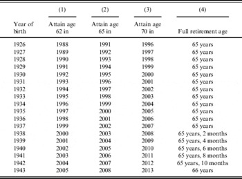
Table 1 shows the FRA for individuals born 1926–43, who will form the sample used in the estimation below. Traditionally, the FRA was 65, so that the month in which an individual attained the FRA always occurred in the calendar year in which the individual turned 65. However, as a result of the 1983 Amendments to the Social Security Act, the FRA was increased by two months for each year of birth from 1938 to 1943 and 1955 to 1960. For those born in the former group, this means that the month in which the individual attains the FRA may fall either in the calendar year in which the individual turns 65 or in the calendar year in which the individual turns 66, depending on the month of birth, which will generate an important source of identifying variation for the earnings-test analysis below.
Full retirement age for individuals born 1926–43

Note: Taken from the 2005 Annual Statistical Supplement, Table 2.A17.1.
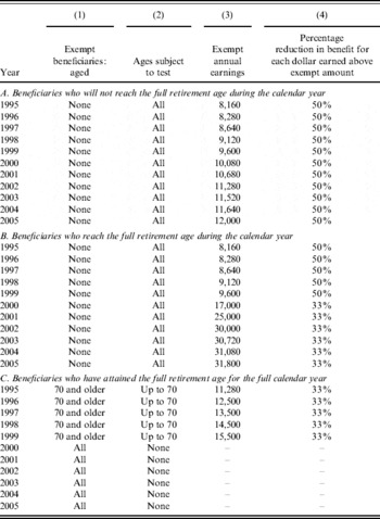
Under the earnings test, reductions in benefits are made in relation to the FRA. As shown in Table 2, prior to 2000, the earnings test reduced benefits $1 for each $2 of annual earnings above an exempt amount, which, for example, was $8,640 in 1997, for beneficiaries under the FRA. For those who had reached the FRA, the earnings test reduced benefits $1 for each $3 of annual earnings above a somewhat higher exempt amount (e.g., $13,500 in 1997).Footnote 3 In addition, there was no earnings test for those who were 70 and older. The 2000 Act abolished the earnings test for those between the FRA and age 70. Any lost benefits are returned to the beneficiary in later years in accordance with the actuarial adjustment and delayed retirement credit, so that, for the population overall, the earnings test is designed to be actuarially fair.
Key earnings – test features, 1995–2005

Note: Taken from the 2005 Annual Statistical Supplement, Table 2.A29.
There are four additional rules that substantially complicate the analysis of the earnings test. First, in the calendar year in which benefits are initially claimed, the earnings test is applied on a month-by-month basis – for the months in which the individual receives benefits – and depends on whether monthly earnings after claiming exceed the monthly exempt amount, which is 1/12th of the annual exempt amount.Footnote 4 If earnings exceed the monthly limit, then benefits are not paid for that month. Second, in the calendar year in which the beneficiary turns 70, the earnings test is applied only to earnings in the months the beneficiary was 69. Third, the 2000 Act created a separate earnings-test category for the calendar year in which the individual attains the FRA. This test applies until the month in which the FRA is reached, after which earnings no longer affect benefit receipt. Each of these special rules implies that even individuals who have the same birth year will be exposed to the earnings test for different lengths of time, according to their month of birth. This generates important sources of variation that are exploited below in the identification strategy. Finally, income from self-employment, though subject to the test, is treated differently than wage income. In particular, self-employment income is counted in the year it is received, rather than the year it is earned. This means the self-employed have the ability to smooth earnings across years, potentially to lessen the burden of the earnings test, in a way that those with wage income cannot.
3 Regression framework and identification strategy
As has been long understood in the literature, there are three broad theoretical partial-equilibrium responses that could have been expected from the repeal of the earnings test from standard models of labor supply when the test is considered a pure tax on earnings. First, there should have been intratemporal, intensive-margin responses for beneficiaries already in the labor force at the time of the law change due to income and substitution effects induced by the repeal. Second, there could have been an extensive-margin (participation) response if there were fixed costs to working, minimum hours' constraints, or other labor-market rigidities that affected older workers.Footnote 5 Finally, there could have been an intertemporal response if individuals shifted their labor supply from years of high to years of low taxation.
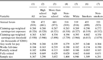
To analyze the overall labor-supply response, we use a sample that consists of all men age 62–72, born between 1926 and 1943, from the 1996, 1998, 2000, 2002, and 2004 waves of the HRS. We exclude two types of person-year observations: those with self-employment income, because of the earnings test rules for such income differ from wage income, and those based on proxy interviews. Overall, this sample consists of 8,367 person-year observations based on 3,765 men. Selected descriptive statistics are shown in Table 3.
Means of selected variables for the sample of men aged 62–72, based on the 1996–2004 waves of the HRS, standard deviations in parentheses

Note: Authors' calculations.
We begin with a basic empirical model that is similar to reduced-form specifications estimated in some previous studies, such as Gruber and Orszag (Reference Gruber and Peter2003)

where i and t index the individual and calendar year, respectively, Y represents a measure of labor supply, κ is a constant, MarStat controls for marital status, Age is measured in years, Interview is the number of months (since January, 1960) in which that HRS wave's interview took place, τ is a set of year effects, and Z is a vector of time-invariant characteristics that includes race, educational attainment, and veteran status.
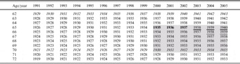
The key explanatory variables are X and T. X is the fraction of the calendar year that the individual was exposed to the earnings test based on the year and month of birth. Specifically, because the repeal treated the earnings of individuals of the same ages (65–70) differently in different calendar years, the 2000 Act induced age-by-time, or year-of-birth, variation in exposure to the earnings test. This is illustrated in Table 4, which depicts the sources of variation due to the repeal for the calendar years covered by the HRS and the years of birth used in this study for a man who claims benefits on his 62nd birthday. Beneficiaries who fall into un-shaded cells were unaffected by the law change. For years of birth in un-shaded cells in italics, the beneficiary was subject to the earnings test for only part of the year, for example, only beginning with the month of birth in the year he turns 62 and ending in the month of birth in the year he turns 70. The year-of-birth variation from the repeal is shown by the shaded rectangle – men aged 65–70 after the law change. For example, beneficiaries in the 1929 cohort were subject to the earnings test every year from ages 62 to 70 under the pre-2000 law. Beneficiaries born five years later, in 1934, were subject to the earnings test in the same manner up through age 65, but not for ages 66–70 because of the repeal.
Illustration of the variation in exposure to the earnings test induced by the repeal for a man who claimed benefits on his 62nd birthday

Notes: Authors' calculations based on the retirement earnings test rules. Each cell shows the year of birth associated with that age and calendar year. Beneficiaries who fall into cells that are not shaded were unaffected by the 2000 Act. Those in un-shaded cells with years of birth in italics indicate that the beneficiary was subject to the earnings test for only part of the year. Beneficiaries affected by the Act are in shaded cells: those affected according to month of birth from the enactment of the new rules for the year in which the full retirement age is attained are shown in bold; those underlined were affected according to month of birth both from the enactment of the new rules for the year in which the full retirement age is attained and the increase in the full retirement age; those in normal font were affected by year of birth; and those in italics were affected according to the month of birth from the abolition of the age-70 rules.
The table also illustrates the variation in exposure due to the month of birth, which has three sources. First, prior to the repeal, beneficiaries who turned 70 were subject to the earnings test for only part of the year, ending in the month of birth in the year they turned 70. For example, those born in April were subject to the test for three months, while those born in October were subject to the test for nine months. After the repeal, beneficiaries who turned 70 were not subject to the test in any month of that year. These are shaded cells in italics in the table. Second, prior to the repeal, all beneficiaries in the year they turned 65 were subject to the earnings test for the entire year, regardless of month of birth, but, after the repeal, similar beneficiaries were subject to the earnings test only until their birth month, generating within-year-of-birth variation in exposure. These are shaded cells in bold in the table. Finally, after the repeal, the earnings test is applied until the beneficiary reaches the full retirement age, but, as documented in Table 1, that age has been increased two months per birth year, for each birth year beginning with 1938. This means that, beginning with that cohort, beneficiaries born in later months of the year were exposed to the earnings test for the entire calendar year they turn 65 and part of the calendar year they turn 66. For example, someone born in December 1937 was exposed for all of year turning age 65, but none of the year turning age 66, while someone born in December 1938 was exposed all of the year turning age 65 and the first two months of the year turning age 66. These cells are shaded cells with underlines. To summarize, the repeal induced across-calendar-year variation in exposure to the earnings test that varied by year of birth, the impact of which was differential by month of birth as well.
We construct the exposure variable, X, to capture these sources of variation. Specifically, let x cmkt be the fraction of the calendar year t a beneficiary who was born in year c, month m, and who claimed benefits at age k was exposed to the earnings test based solely on the legislative variation in earnings-test rules. Because the earnings test may have affected claiming behavior, we do not want to use the value of x associated with the individual's actual claiming age.Footnote 6 Instead, we take a weighted average of x, weighting the claiming-age-specific exposure by the distribution of claiming ages for the 1926 cohort taken from the various issues of the Annual Statistical Supplement to yield a claiming-age-weighted exposure, X. That is, let Pr(R 1926k) be the probability of claiming retirement benefits at age k for the 1926 cohort; then the key explanatory variable is
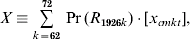
and ranges from zero to one.Footnote 7
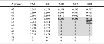
Table 5 shows the sample mean of X and illustrates the age-by-calendar-year, or year-of-birth, variation in exposure to the earnings test for the years covered in our HRS sample. Prior to the 2000 Act, X rises with age. For 1996, it peaks at 0.983 for age 69 and does not attain 1, because there is some positive probability the worker will claim after age 69. There is no earnings test for those older than 70, so X is zero for those ages. The impact of the repeal is apparent, as exposure falls to zero for 66–70 year olds starting in 2000. For 65 year olds, X falls from 0.8 in 1998 to 0.3 in 2000, i.e. half a year less exposure, but then rises in 2004 to 0.5 because the increase in the full retirement age raises the number of months in the year some individuals are subject to the test. Overall, there is substantial variation in exposure to the earnings test induced by the 2000 Act.
Sample mean claiming-age-weighted exposure to the earnings test by age and calendar year

Notes: Authors' calculations based on the retirement earnings test rules and the analysis sample. Each cell shows the mean of the claiming-age-weighted exposure variable described in the text. Beneficiaries who fall into un-shaded cells were unaffected by the 2000 Act. Those in un-shaded cells in italics were subject to the earnings test for only part of the year. Beneficiaries affected by the Act are in the shaded cells: in bold are those affected according to month of birth from the enactment of the new rules for the year in which the full retirement age is attained; underlined are those affected according to month of birth both from the enactment of the new rules for the year in which the full retirement age is attained and the increase in the full retirement age; those affected by year of birth only are shown in normal font; and those affected according to the month of birth from the abolition of the age-70 rules are shown in italics.
Similarly, T is the claiming-age-weighted real earnings-test threshold, based on the thresholds given in Table 2, but expressed in thousands of $2001. It is positive for years for which the individual faced the earnings test and is zero for years in which the individual was exempted from the test. Hence, there is an implicit interaction between X and T.
Recent studies that have focused on labor supply, such as Gruber and Orszag (Reference Gruber and Peter2003), Friedberg and Webb (Reference Friedberg and Anthony2006), and Haider and Loughran (Reference Haider and Loughran2008), have used just the year-of-birth variation in their analyses. Using either individual data or age-by-year cell-level data, they have estimated specifications like (1), employing a dummy variable that takes on a value of one if subject to the earnings test and zero otherwise and the real value of the threshold as the key explanatory variables, but without accounting for potentially finer differences in incentives associated with different claiming ages.
In contrast, because we exploit both the year- and month-of-birth variation, and the HRS provides panel data on individuals two years apart, we estimate our model on individual data in first differences

where the dependent variable, ΔY it≡Y it−Y it−2, measures the change in the labor-supply outcome in the last two years, α≡2δ, υ≡Δu, γ≡Δτ is a set of calendar-year effects, ΔMarStat indicates a change in marital status in the last two years, and ΔInterview indicates the number of months elapsed since the last interview. The key identifying assumption is that the variation in ΔX and ΔT induced by the repeal of the earnings test is plausibly exogenous with respect to the trajectory of the unobserved variable(s), including any measurement error, embodied in υ. Because of the implicit interaction between the threshold variable, T, and the exposure variable, X, the key parameters that measure the average effect of the repeal on labor supply are β1 and β2. The focal statistical test is of the null hypothesis that the repeal had no impact on labor supply: β1=β2=0. Furthermore, we calculate the marginal effect of the repeal on labor supply as −β1−β2⋅ , where =16.841, the 1999 (pre-repeal) nominal threshold of $15,500 from Table 2 for those who had attained the FRA, which was $16,841 in real terms (and expressed in thousands).
4 Estimation results for all men
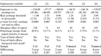
The first two rows in Table 6 show the ordinary least squares (OLS) estimates of β1 and β2 in (3) for annual hours, respectively. Column 1 shows estimates for the baseline model:  and
 . As the exposure measure varies by year and month of birth and calendar year, and the HRS panel yields multiple observations on the same individual, the standard errors (in parentheses) are calculated using the robust multi-way cluster variance-covariance estimator of Cameron et al. (Reference Cameron, Gelbach and Miller2006). Because of the prospect of temporal and across-year-of-birth correlation in outcomes (Bertrand et al., Reference Bertrand, Esther and Sendhil2003), we cluster only on the month of birth and the individual. Based on the p-value of 0.0001 shown in the third row, the null hypothesis that the earnings test had no effect on labor supply can be rejected. The estimated marginal effect of the repeal was to raise labor supply by 228 hours, which, when compared to mean hours, represented a 43.8% increase in hours supplied.Footnote 8
OLS parameter estimates of the repeal of the retirement earnings test on the annual hours of all men aged 62–72, based on the 1996–2004 waves of the HRS, standard errors in parentheses

Notes: Each column gives selected results from a separate OLS estimation of equation (3) in the text when the labor-supply outcome (dependent variable) is annual hours. Standard errors are in parentheses and are calculated using the robust multi-way cluster variance-covariance estimator of Cameron et al. (Reference Cameron, Gelbach and Miller2006), clustered on the month of birth and the individual.
One factor that could confound the baseline estimates is the presence of year-of-birth-specific heterogeneity in dynamic patterns of work behavior that were changing over time and just happened to be correlated with the variation in incentives from the repeal of the earnings test. Friedberg and Webb (Reference Friedberg and Anthony2006) offer an example of this. In particular, they argue that part of the variation in labor-market behavior of older individuals from 1996–1999 – the pre-repeal period in the current paper – was an intertemporal response to actual and anticipated changes in the earnings-test threshold enacted in the 1996, which would have raised the exempt amount to $17,000, $25,000, $30,000, $30,720, in 2000–2003 in nominal terms, respectively, but were never put into place because the 2000 Act superseded the 1996 changes. To account for this, column 2 presents estimates from the preferred specification: equation (3) with a full set of year-of-birth dummies included, which allows changes in hours to vary systematically across years of birth, but in a way that is constant across calendar years.Footnote 9 In so doing, the estimates of β1 and β2 are identified off of the differential variation across periods in the year-of-birth-specific incentives from the repeal, as well as the differential month-of-birth variation. This greatly reduces the estimated impact of the repeal. Now, the repeal increased annual hours by an estimated 71 hours, which represented a 13.7% increase.
Column 3 pushes this robustness check further by adding interactions of year-of-birth effects with a linear time trend. This allows changes in hours to vary systematically across years of birth, but in a way that is changing (smoothly) across calendar years. In so doing, much of the legislative variation is no longer used, and the estimates of β1 and β2 now are identified primarily off of the differential month-of-birth variation and, to a much lesser extent, variation in the year-of-birth-specific incentives from the repeal that is non-linear across time. A comparison of columns 2 and 3 show that the addition of trend interactions changes the parameter estimates very little. This suggests that any time-trending omitted year-of-birth factors are not imparting bias to the estimates. As expected, though, the precision falls, because we have parsed out much of the legislative variation. Now, the repeal increased annual hours by an estimated 85 hours, which represented a 16.3% increase.
The remaining results in the table are additional robustness checks. In column 4, 2% of the sample has been trimmed from each tail of the change-in-hours' distribution in order to reduce the potential impact of measurement error. This has the effect of reducing the estimated labor supply response: hours rose 8.1% with the repeal. The results in columns 5 and 6 further check the robustness of the findings to both measurement error and longer-run trends in labor supply employing four-year rather than two-year differencing to the specifications (Griliches and Hausman, Reference Griliches and Hausman1986). These specifications indicate that the earnings-test repeal raised labor supply by 92–107 hours per year, or 17.9–21.1%.Footnote 10
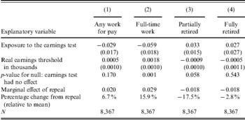
Because some of the response could have occurred on the extensive (participation) margin and there are a variety of ways in which older individuals characterize their labor-market attachment (Gustman et al., Reference Gustman, Mitchell and Steinmeier1995), we present estimates in Table 7 for four alternative measures of labor supply: whether the individual does any work for pay, works full-time, and whether the individual reports in the survey that he is partially and fully retired, respectively. In column 1, those who reported working for pay rose by 2 percentage points, or 6.7% (relative to the mean participation rate of 29.9%). However, based on the p-value of 0.17, there is no statistically significant evidence that labor-force participation rose with the repeal. Instead, from column 2, it appears that the response was associated with an increase in full-time work: those engaged in full-time work rose by 2.9 percentage points, or 16%. Similarly, those who reported being partially retired fell 1.8 percentage points, or 17.5%.
OLS parameter estimates of the impact of the repeal of the retirement earnings test on various measures of labor force participation of men aged 62–72, based on the 1996–2004 waves of the HRS and two-year differencing, standard errors in parentheses

Notes: Each column gives selected results from a separate OLS estimation of equation (3) in the text when the labor-supply outcome (dependent variable) is that shown in the column heading. Standard errors are in parentheses and are calculated using the robust multi-way cluster variance–covariance estimator of Cameron et al. (Reference Cameron, Gelbach and Miller2006), clustered on the month of birth and the individual.
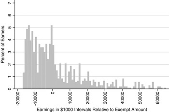
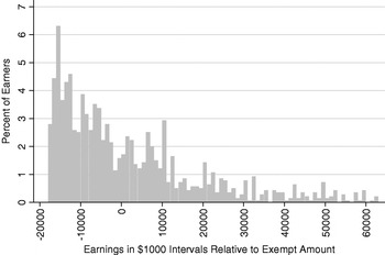
To help corroborate these initial labor-supply findings, Figure 1A shows the distribution of real earnings (in $2001) taken from the income section of the HRS survey relative to the exempt amount in intervals of $1,000 for men 65–70 years old and in the labor force prior to the repeal.Footnote 11 The value of zero on the horizontal axis indicates that annual earnings equaled the exempt amount; a negative value means that earnings were less than the exempt amount; a positive value means that earnings were greater than the exempt amount. The figure shows that the bulk of earnings were below the exempt amount, and, more specifically, bunching at the exempt amount.
Earnings Distribution of 65–70 Year Olds Before 2000

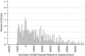
In comparison, Figure 1B shows the real earnings distribution after the repeal. For this figure, earnings are shown relative to a counterfactual exempt amount, namely the nominal 1999 exempt amount ($15,500) indexed by the national wage index for the years 2000–2003 and then deflated into real terms. There is no evidence of bunching after the repeal. The p-value for the Kolmogorov–Smirnov test of the equality of the earnings distributions in these figures is 0.001. This suggests that the earnings test for those above the FRA was binding prior to the repeal.Footnote 12
Earnings Distribution of 65–70 Year Olds After 2000

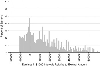
This conclusion is bolstered by Figures 2A and 2B, which show the real earnings distributions for a comparison group of men – those in the labor force, aged 62–64, for whom the earnings test was unchanged – before and after 2000, respectively. For this younger group of men, the real earnings distributions are very similar before and after the law change, both showing evidence of bunching at the exempt amount.Footnote 13 The p-value for the Kolmogorov–Smirnov test of the equality of the earnings distributions in Figures 2A and 2B is 0.751.
Earnings Distribution of 62–64 Year Olds Before 2000

Earnings Distribution of 62–64 Year Olds After 2000

5 Estimates for sub-groups based on correlates with discount rates
One well-known theoretical prediction is that the repeal should have had a differential impact on labor supply based on individual discount rates. Specifically, under the test, any lost benefits are returned to the beneficiary in later years in accordance with the actuarial adjustment and delayed retirement credit, both of which are designed to be ‘actuarially fair’ for the older population as a whole. However, as long as individual discount rates vary substantially, the test will not necessarily be actuarially fair for sub-groups of the older population.
To see this, consider a simple two-period framework for someone who has claimed benefits. In the first period, the individual can work H hours at the gross wage rate, w, and receive benefits, B, but is subject to the test; in the second period, the individual only receives benefits. The present value of total income, Y, to the individual is
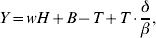
where T is the amount of benefits that are clawed back (taxed) by the test and will be a function of earnings, wH. Those lost benefits are returned in the next period at a rate of adjustment of δ⩾1, but are discounted back to the present by the individual's discount rate, including mortality risk, of β⩾1. For the purposes of illustration, let T be a twice continuously differentiable function of earnings, then the return from an additional hour of work is
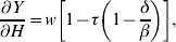
where τ is the claw-back (tax) rate.
For individuals whose discount rate equals the adjustment rate, β=δ, the return is just the gross wage. They are indifferent between additional earnings in the present and additional benefits in the future. For those whose discount rate is greater than the adjustment rate, β>δ, the earnings test reduces the return to work, and, conversely, the return to work rises with the repeal. Therefore, empirically we should expect to see differential labor-supply responses according to discount rates, which will vary across individuals due to differences in mortality risk, the pure rate of time preference, and liquidity constraints.
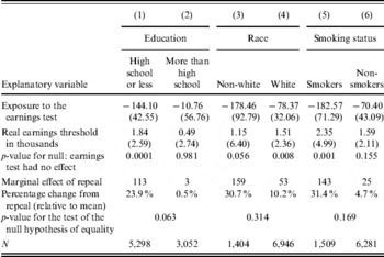
Table 8 presents estimates for annual hours that test this theoretical prediction. Although we do not have direct measures of mortality risk, pure rates of time preference, and liquidity constraints, for the purposes of the test, we split the sample according to exogenous proxy variables. Specifically, in columns 1–2 of the table, we split the sample by education (high school or less and more than high school) and estimate the response to the repeal in each sub-sample separately. Similarly, we do this by race (white and non-white) and smoking status (smoker and non-smoker) in columns 3–6, repsectively. Race and education are correlated with mortality risk (Hurd and McGarry, Reference Hurd and Kathleen1995; Kitigawa and Hauser, Reference Kitagawa and Hauser1973); race and education are correlated with liquidity constraints (Jappelli, Reference Jappelli1990; Hurst and Charles, Reference Hurst and Kofi2002); and education and smoking status are correlated with time preference (Grossman, Reference Grossman, Cuyler and Newhouse2000).
OLS parameter estimates for sub-groups by education, race, and smoking status of the impact of the repeal of the retirement earnings test on the annual hours of men aged 62–72, based on the 1996–2004 waves of the HRS, two-year differencing on the untrimmed sample, standard errors in parentheses

Notes: Each column gives selected results from a separate OLS estimation of equation (3) in the text when the labor-supply outcome (dependent variable) is annual hours for the sub-sample shown in the column heading. Standard errors are in parentheses and are calculated using the robust multi-way cluster variance-covariance estimator of Cameron et al. (Reference Cameron, Gelbach and Miller2006), clustered on the month of birth and the individual.
Broadly speaking, the results in the table are consistent with the prediction. Much of the labor-supply response is centered on those with high discount rates – the lesser educated, non-whites, and smokers – who find the deferral of benefits under the earnings test relatively disadvantageous. Specifically, the estimated marginal effect of the repeal was an increase in labor supply of an estimated 113 hours, or 23.9%, for those with a high school degree or less, but only three hours (0.5%) for those with more than a high school degree. This is significant at the 6.3% level, based on the next-to-last row in the table, which shows the p-value for the test of the null hypothesis of equality between the two groups. Based on sample mean hours and the number of men in each of these groups, essentially all (100%) of the total change in hours from the repeal originates from lesser educated men.
Non-whites increased hours by an estimated 159 hours (30.7%), compared to only 53 hours (10.2%) for whites. Annual hours rose by an estimated 143 hours (31.4%) for smokers, but only 25 hours (4.7%) for non-smokers. These are economically large differences in response between groups, generally consistent with the theoretical prediction; however, the precision of the estimation is such that the null of equality cannot be rejected at conventional significance levels.
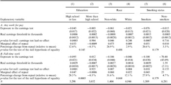
Table 9 repeats this analysis for two of the alternative labor-supply measures from Table 7, work for pay and full-time work. In panel A, there were economically substantial increases in the fraction of older men who reported working for pay after the repeal of the earnings test for the lesser educated, non-whites, and smokers, but no such responses for the other groups. The fact that labor-force participation responded to the repeal suggests that there are significant labor-market rigidities for older men, consistent with the findings of Baker and Benjamin (Reference Baker and Benjamin1999) and Haider and Loughran (Reference Haider and Loughran2008), among others. However, the estimates are not precise enough to reject the null of equality, based on the p-values in the last row of the panel. In panel B, there were economically and statistically significant increases in the fraction of older men working full-time after the repeal that again were concentrated among older men who were the lesser educated and non-whites.
OLS parameter estimates for sub-groups by education, race, and smoking status of the impact of the repeal of the retirement earnings test on various measures of labor force participation of men aged 62–72, based on the 1996–2004 waves of the HRS with two-year differencing, standard errors in parentheses
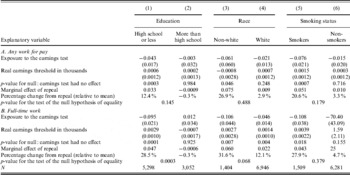
Notes: Each column of each panel gives selected results from a separate OLS estimation of equation (3) in the text when the labor-supply outcome (dependent variable) is that shown in the panel heading for the sub-sample shown in the column heading. Standard errors are in parentheses and are calculated using the robust multi-way cluster variance–covariance estimator of Cameron et al. (Reference Cameron, Gelbach and Miller2006), clustered on the month of birth and the individual.
6 Conclusion
In summary, the repeal of the earnings test was associated with a substantial increase in the labor supply of older men. Our estimates based on variation in exposure to the earnings test that includes year of birth, as previous studies have done, suggest a substantial increase in annual hours associated with the repeal: pooled over all men, hours rose by about 44%. However, when we use our new measure of exposure that uses variation both by month and year of birth, and we explicitly control for year-of-birth effects and trends, the increase in annual hours associated with the repeal is much smaller: pooled over all men, hours rose by about 15%. This suggests that omitted year-of-birth-specific effects and trends in labor supply may have imparted substantial bias to previous estimates of the impact of the earnings test.
In other results, we found that the repeal increased labor force participation, and much of the increase in labor supply was associated with a rise in the incidence of full-time work. Although the estimation results were not always very precise, the broad pattern of estimates suggest that much of the labor-supply response was concentrated among men with characteristics correlated with high discount rates – the lesser educated, non-whites, and smokers – who may have found the incentives to work under the earnings test particularly disadvantageous. These individuals greatly increased their labor supply after the repeal, between 25 and 30%.
In comparison to structural approaches, our results are larger than the labor-supply increase of 5% from the repeal of the earnings test for 65–70 year olds simulated based on the structural estimates of Friedberg (Reference Friedberg2000), who used CPS data on earlier earnings-test reforms and non-linear budget-set techniques to model the earnings test as a pure tax on earnings, but much smaller than the simulated effects in French (Reference French2005), whose estimates based on earlier PSID data predicted an increase of 400 hours per year from the repeal. Overall, our findings are qualitatively consistent with those of Haider and Loughran (Reference Haider and Loughran2008), Tran (Reference Tran2004), Song (Reference Song2004), and Song and Manchester (Reference Song and Joyce2007). In combination, these studies suggest an important labor supply response from the 2000 Act.