





1. Introduction
Dense suspensions of Brownian and non-Brownian solid particles in viscous liquid present intriguing flow properties, and understanding their rheology is a subject of both fundamental and technological relevance (Stickel & Powell Reference Stickel and Powell2005; Ness, Seto & Mari Reference Ness, Seto and Mari2022). Of particular interest are suspensions comprising particles with radius  $a\approx 1$
 $\mathrm {\mu }$m, or more broadly in the range 0.1–10
 $\mathrm {\mu }$m. These are present in numerous applications, in all areas of food science (Jambrak et al. Reference Jambrak, Herceg, Šubarić, Babić, Brnčić, Brnčić, Bosiljkov, Čvek, Tripalo and Gelo2010) and consumer products, as well as across the manufacturing and construction sectors (Roussel et al. Reference Roussel, Lemaître, Flatt and Coussot2010) and indeed in many geophysical contexts (Kostynick et al. Reference Kostynick, Matinpour, Pradeep, Haber, Sauret, Meiburg, Dunne, Arratia and Jerolmack2022). Often their physics are challenging because their Brownian diffusion time may be comparable to the processing or macroscopic time scales involved in their use, so that they sit at the boundary of colloidal and granular systems (Guy, Hermes & Poon Reference Guy, Hermes and Poon2015).
Particle-based simulation offers a promising route to better understand the physics of these materials, providing highly resolved information complementary to what can be obtained by experiment. With simultaneous access to particle trajectories and bulk rheology, one might devise new micromechanical constitutive equations (Gillissen et al. Reference Gillissen, Ness, Peterson, Wilson and Cates2020) or develop microstructural insight that could guide the future analysis of experimental data. Numerical models might also be useful for exploring the parameter space and systematically linking aspects of particle-level physics (friction (Seto et al. Reference Seto, Mari, Morris and Denn2013), adhesion (Richards et al. Reference Richards, Guy, Blanco, Hermes, Poy and Poon2020) and roughness (Lobry et al. Reference Lobry, Lemaire, Blanc, Gallier and Peters2019)) to the bulk flow behaviour. As a result, one might aim to optimise industrial processes such as mixing and extrusion, or indeed to optimise the design of the materials themselves through additives, using insight gained through particle-based simulation.
Stokesian dynamics (SD) (Brady & Bossis Reference Brady and Bossis1988; Banchio & Brady Reference Banchio and Brady2003) is a computational method used to simulate the rheological behaviour of colloidal and granular particles suspended in a viscous fluid, addressing the special case of inertia-free flow where the Stokes number is zero (Ermak & McCammon Reference Ermak and McCammon1978). The latter quantity is similar to a Reynolds number, and is defined as the ratio between the shearing time scale  $1/\dot {\gamma }$ and
 $\rho a^2/\eta$, with
 $\dot{\gamma}$ the shear rate,
 $\rho$ the particle density (assumed equal to that of the fluid in the remainder of this article),
 $a$ the particle size and
 $\eta$ the liquid viscosity. Other forms of Reynolds number may be defined, for instance based on the fluid density (if it differs from that of the particles) or on another length scale. In the limit of zero Stokes number, analytical solutions of the Stokes equation of motion can be used to derive particle-scale hydrodynamic interactions. The SD method involves balancing all of the forces and torques on each particle by evaluating their velocities via a grand mobility matrix containing information on the relative positions of every particle in the system, ensuring conservation of translational and angular momentum. Despite accurately capturing the long- and short-range hydrodynamic interactions between particles, SD has not been adopted widely as a predictive tool in applied and industrial settings in the same way as other particle-based simulation methods have, due to the complexity of its implementation and its computational expense (notwithstanding recent developments that significantly speed it up (Sierou & Brady Reference Sierou and Brady2001; Fiore & Swan Reference Fiore and Swan2019)).
The discrete element method (DEM) (Cundall & Strack Reference Cundall and Strack1979), on the other hand, is a particle-based computational method (a variant of molecular dynamics) that is used widely to simulate the behaviour of granular materials including powders, particles and grains, taking into account their pairwise interactions. In contrast to SD, DEM does not explicitly balance the forces on each particle. Instead, inertia is present, and one simply sums the forces and torques and the resultant leads to linear and rotational accelerations that can be realised through a conventional timestepping algorithm such as velocity-Verlet. This approach has proven to be useful for studying overdamped suspensions under shear flow (Trulsson, Andreotti & Claudin Reference Trulsson, Andreotti and Claudin2012; Ness & Sun Reference Ness and Sun2015), where one introduces short-ranged lubrication forces and sets the Stokes number to be  $O(10^{-2})$ or smaller (assuming that hydrodynamic force and torque interactions derived in the limit of zero Stokes number still apply). Moreover, it is pragmatic in the sense that the physics associated with flowing dense suspensions can be implemented in existing, widely used codes with large user bases, so that they have a clear path to adoption in engineering and other applied contexts. To date, there is not, to our knowledge, an open-source DEM simulation that includes the relevant physics of dense suspensions at the colloidal-to-granular interface, accounting for short-ranged hydrodynamics, Brownian forces and (frictional) particle–particle contacts.
Here, we present a minimal particle-based simulation model for predicting the rheology of dense Brownian and non-Brownian suspensions. Our model comprises hydrodynamic lubrication, particle–particle contacts and Brownian forces. After first describing the model in detail, we present some aspects of the effective interactions and diffusion that arise, before giving a detailed account of the rheological predictions of the model. The model reproduces well the main features of the experimentally observed rheology of dense suspensions, namely a low shear rate plateau that gives way to shear thinning and later shear thickening as the shear rate is increased, with the relative viscosity of the suspension increasing sharply with solid volume fraction and particle–particle friction coefficient.
2. Methodology
We consider a model system of nearly monodisperse solid spheres, dispersed at high solids volume fraction  $\phi$ in a density-matched Newtonian liquid. The microscopic physics included in our model represents a minimal set of ingredients necessary to make useful predictions of the rheology of suspensions comprising particles with radius in the range
 $10^{-7}$ to
 $10^{-4}$ m. The trajectories of individual particles with translational and rotational motion are governed by Langevin equations that comprise three force (
 $\boldsymbol {F}$) and torque (
 $\boldsymbol {T}$) contributions: direct particle contacts (
 $\boldsymbol {F}^{C}$,
 $\boldsymbol {T}^{C}$), hydrodynamics (
 $\boldsymbol {F}^{H}$,
 $\boldsymbol {T}^{H}$) and Brownian noise (
 $\boldsymbol {F}^{B}$,
 $\boldsymbol {T}^{B}$). The equations of motion for the translation and rotation of the particles are written, respectively, as
 $$\begin{gather} m_i\frac{{\rm d}^2\boldsymbol{x}_i}{{\rm d}t^2} = \sum_j\boldsymbol{F}_{i,\,j}^{C} + \boldsymbol{F}_{i}^{H,D} + \sum_j\boldsymbol{F}_{i,\,j}^{H,L} + \boldsymbol{F}_{i}^{B,D} + \sum_j\boldsymbol{F}_{i,\,j}^{B,L}, \end{gather}$$
 $$\begin{gather}\frac{2}{5}m_ia_i^2\frac{{\rm d}\boldsymbol{\varOmega}_i}{{\rm d}t} = \sum_j\boldsymbol{T}_{i,\,j}^{C} + \boldsymbol{T}_{i,\,j}^{H,D} + \sum_j\boldsymbol{T}_{i,\,j}^{H,L} + \boldsymbol{T}_{i,\,j}^{B,D} + \sum_j\boldsymbol{T}_{i,\,j}^{B,L} , \end{gather}$$
where  $\boldsymbol {x}_i$ represents the position of particle
 $i$,
 $\boldsymbol {\varOmega }_i$ represents its rotational velocity and
 $a_i$ and
 $m_i$ are its radius and mass, respectively. The subscript
 $i$ represents single-body forces and torques acting on particle
 $i$, while the subscript
 $i,\,j$ represents pairwise forces and torques acting between particles labelled
 $i$ and
 $j$. The superscripts C, H, B, D and L refer to the force and torque components arising due to contacts (C), hydrodynamics (H) and Brownian (B) effects, with the latter two acting both through drag (D) and lubrication (L). Each of these force and torque terms is described in detail below. These equations of motion can be understood as Langevin equations in which the
 $\langle {\cdot }\rangle ^C$ terms represent particle–particle interactions; the
 $\langle {\cdot }\rangle ^H$ terms represent configuration-dependent viscous friction (i.e. dissipative forces linear in the particle velocities); and the
 $\langle {\cdot }\rangle ^B$ terms represent configuration-dependent (multiplicative) noise. Although particle inertia is present in the model, we omit fluid inertia (Hinch Reference Hinch1975), arguing that, for the regimes of interest, the principal contributions to the overall bulk rheology will come from particle–particle contact and hydrodynamic lubrication interactions. Particles are subjected to a liquid flow field given by
 $\boldsymbol {U}^\infty$ (acting through the body force
 $\boldsymbol {F}^{H,D}_i$ as described below), leading to a rate of strain tensor
 $\mathbb {E}=\frac {1}{2}(\boldsymbol {\nabla }\boldsymbol {U}^\infty + (\boldsymbol {\nabla }\boldsymbol {U}^\infty )^{T})$. Pairwise forces and torques are summed over the neighbours
 $j$ of each particle
 $i$, and the positions, velocities and acceleration are updated in a stepwise manner following the velocity-Verlet algorithm (Swope et al. Reference Swope, Andersen, Berens and Wilson1982; Frenkel & Smit Reference Frenkel and Smit2023). Below, we describe each of the force and torque contributions in detail; shown in figure 1 are illustrative schematics of each of the forces.
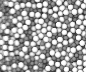
Snapshot of simulation box, and schematics of the leading pairwise force terms present in the model. In all cases, the leading component of the pairwise force acts along the (positive or negative) direction of the unit vector  $\boldsymbol {n}_{i,\,j}$ pointing from the centre of particle
 $i$ to the centre of particle
 $j$. (a) Snapshot of the simulation box showing particles of radii
 $a$ (blue) and
 $1.4a$ (red), and the cubic domain length
 $L$. Particles are mixed in approximately equal volume. We used a minimum particle number
 $N=1000$ (
 $L\approx 25a$) to ensure statistically significant results. (b) Contact force, with force acting along
 $\boldsymbol {n}_{i,\,j}$; shown from left to right are (i) sketch of contacting particles
 $i$ and
 $j$, with the overlap
 $\delta _{i,\,j}$ shown in green; (ii) the unit vector
 $\boldsymbol {n}_{i,\,j}$ pointing from the centre of particle
 $i$ to
 $j$; (iii) repulsive contact
 $F^C$ forces acting along the positive and negative directions of
 $\boldsymbol {n}_{i,\,j}$. (c) Pairwise hydrodynamic lubrication force, with force set by the component of the relative particle velocity acting along
 $\boldsymbol {n}_{i,\,j}$; shown from left to right are (i) sketch showing the velocity vectors
 $\boldsymbol {U}$ of neighbouring particles
 $i$ and
 $j$; (ii) the relative velocity
 $U_j-U_i$ breaks down into tangential (blue) and normal (red) components, with the latter pointing along
 $\boldsymbol {n}_{i,\,j}$; (iii) lubrication forces act along the positive and negative directions of
 $\boldsymbol {n}_{i,\,j}$, proportional to the normal part of the relative velocity. (d) Pairwise Brownian lubrication force with a random pairwise vector
 $\boldsymbol {\theta }_{i,\,j}$ projected onto
 $\boldsymbol {n}_{i,\,j}$. Shown from left to right are (i) neighbouring particles with centre-to-centre unit vector
 $\boldsymbol {n}_{i,\,j}$; (ii) random vectors
 $\boldsymbol {\theta }_{i,\,j}$ drawn from a Gaussian distribution (green) are projected onto
 $\boldsymbol {n}_{i,\,j}$ by the tangential (blue) and normal (red) operators; (iii) Brownian forces act along the positive and negative directions of
 $\boldsymbol {n}_{i,\,j}$, proportional to the normal part of the random vector.

2.1. Contact forces and torques
The particle–particle contact force  $\boldsymbol {F}^C$ follows a conventional granular-type interaction (Cundall & Strack Reference Cundall and Strack1979), and is activated for any two particles
 $i$ and
 $j$ for which the centre-to-centre distance
 $|\boldsymbol {r}_{i,\,j}|$ is smaller than the sum of the radii
 $a_i + a_j$. Contact forces include a repulsive part acting normal to the pairwise centre-to-centre vector
 $\boldsymbol {r}_{i,\,j}$ (we define a unit vector
 $\boldsymbol {n}_{i,\,j} = \boldsymbol {r}_{i,\,j}/|\boldsymbol {r}_{i,\,j}|$), and a tangential part. For simplicity, we model contacts as linear springs, so that particle pairs experience repulsive contact forces proportional to their scalar overlap, defined once in contact as
 $\delta _{i,\,j} = (a_i+a_j)-|\boldsymbol {r}_{i,\,j}|$. The implementation of our model within LAMMPS (Plimpton Reference Plimpton1995) nonetheless allows straightforward deployment of more complex
 $\delta _{i,\,j}$ dependence (we note that, in LAMMPS, the skin argument of the neighbour command has units of (length)). Tangential forces are linear in
 $\boldsymbol {\xi }_{i,\,j}$, a vector describing the accumulated displacement of the particle pair perpendicular to
 $\boldsymbol {n}_{i,\,j}$ since the initiation of the contact. Contact force and torque magnitudes are controlled by normal and tangential stiffness constants
 $k_n$ and
 $k_t$ that set the hardness of the particles. The force and torque are given, respectively, by
 $$\begin{gather} \boldsymbol{F}_{i,\,j}^{C}=k_n\delta_{i,\,j} \boldsymbol{n}_{i,\,j}-k_t\boldsymbol{\xi}_{i,\,j}, \end{gather}$$
 $$\begin{gather}\boldsymbol{T}_{i,\,j}^{C}=a_i(\boldsymbol{n}_{i,\,j} \times k_t\boldsymbol{\xi}_{i,\,j}) . \end{gather}$$
We additionally introduce a static friction coefficient  $\mu$ that constrains the tangential force to
 $|k_t\boldsymbol {\xi }_{i,\,j}|\leq \mu k_n\delta _{i,\,j}$. For larger values of
 $k_t\boldsymbol {\xi }_{i,\,j}$, the tangential part of the force and the torque are truncated, and particle contacts transition from a rolling to a sliding regime. We present data for
 $\mu =0$ throughout, except in figure 6, where we explore the role of contact friction. Damping is not included in
 $\boldsymbol {F}_{i,\,j}^{C}$ or
 $\boldsymbol {T}_{i,\,j}^{C}$ as the lubrication forces and torques described below already render particle–particle contacts well within the overdamped regime. Each pairwise contact between particles
 $i$ and
 $j$ contributes to the overall contact stress of the system with a tensorial stresslet given by the outer product
 $-\boldsymbol {F}^{C}_{i,\,j} \otimes \boldsymbol {r}_{i,\,j}$. The contact stress
 $\unicode{x2140}^C$ is obtained by summing this quantity over all contacting particle pairs and dividing by the system volume and dimension.
Contact forces of this kind have successfully been deployed in numerical models for rate-independent granular suspension rheology (Boyer, Guazzelli & Pouliquen Reference Boyer, Guazzelli and Pouliquen2011; Trulsson et al. Reference Trulsson, Andreotti and Claudin2012; Cheal & Ness Reference Cheal and Ness2018; Ge & Brandt Reference Ge and Brandt2020) and for models of shear thickening suspensions (Seto et al. Reference Seto, Mari, Morris and Denn2013) (in the latter case, rate dependence arises from a ‘critical load’ that the contact force must exceed before static friction is activated).
2.2. Hydrodynamic forces and torques
In general, hydrodynamic interactions in suspensions appear as single-particle drag forces  $\boldsymbol {F}^{H,D}$, pairwise near-contact lubrication forces
 $\boldsymbol {F}^{H,L}$ and many-body long-range forces. In high volume fraction dense suspensions, however, it is argued by many authors that the hydrodynamic interactions are dominated by near-contact lubrication interactions (Ball & Melrose Reference Ball and Melrose1997) (which diverge on close approach) and that long-range interactions are effectively screened by intervening particles (Seto et al. Reference Seto, Mari, Morris and Denn2013; More & Ardekani Reference More and Ardekani2020). We follow this reasoning and therefore omit long-range hydrodynamics from our model, although we note there exist several implementations of coupling schemes between LAMMPS and fluid solvers that extend the capability down to dilute and semi-dilute regimes (see e.g. Sun & Xiao Reference Sun and Xiao2016). Below, we describe in detail the drag and lubrication forces deployed in the model. Single-particle drag forces and torques are given by
 $$\begin{gather} \boldsymbol{F}^{H,D}_{i}=6{\rm \pi}\eta a_i (\boldsymbol{U}^\infty(\boldsymbol{x}_i)-\boldsymbol{U}_i), \end{gather}$$
 $$\begin{gather}\boldsymbol{T}^{H,D}_{i}=8{\rm \pi}\eta a^3_i (\boldsymbol{\varOmega}^\infty-\boldsymbol{\varOmega}_i) , \end{gather}$$
where we use the isolated-particle Stokes terms and, for simplicity, do not introduce volume-fraction-dependent hindrance functions. Here,  $\eta$ is the liquid viscosity,
 $\boldsymbol {U}^\infty (\boldsymbol {x}_i)$ is the value of the liquid streaming velocity at the position of the centre of mass of particle
 $i$, and
 $\boldsymbol {\varOmega }^\infty = \frac {1}{2}(\boldsymbol {\nabla }\times \boldsymbol {U}^\infty )$ (spatially uniform assuming
 $\boldsymbol {U}^\infty$ varies linearly in space). The drag forces lead to a per particle stress given by
 $\unicode{x2140}^{H,D}_i = \frac {20}{3}{\rm \pi} \eta a_i^3\mathbb {E}$.
For pairwise lubrication forces and torques acting between interacting particles  $i$ and
 $j$ we start from the conventional representation given by Kim & Karrila (Reference Kim and Karrila2013) as
 \begin{equation} \begin{pmatrix}
\boldsymbol{F}_{i,\,j}^{H,L} \\ \boldsymbol{F}_{j,i}^{H,L} \\
\boldsymbol{T}_{i,\,j}^{H,L} \\ \boldsymbol{T}_{j,i}^{H,L}\\
\unicode{x2140}_{i,\,j}^{H,L}\\ \unicode{x2140}_{j,i}^{H,L}
\end{pmatrix} =\eta{\mathbb{R}} \begin{pmatrix}
\boldsymbol{U}^\infty(\boldsymbol{x}_i)-\boldsymbol{U}_i \\
\boldsymbol{U}^\infty(\boldsymbol{x}_j)-\boldsymbol{U}_j \\
\boldsymbol{\varOmega}^\infty-\boldsymbol{\varOmega}_i \\
\boldsymbol{\varOmega}^\infty-\boldsymbol{\varOmega}_j \\
\mathbb{E}\\ \mathbb{E} \end{pmatrix},
\end{equation}
where  ${\mathbb {R}}$ is the resistance matrix containing tensorial operations that linearly couple pairwise particle forces (torques) to velocities (rotational velocities), taking into account relative particle positions. After some algebra and omitting terms that vanish with the size of the interparticle gap (see Radhakrishnan Reference Radhakrishnan2018 for details) one can obtain the forces in a simplified pairwise form as
 \begin{align} \boldsymbol{F}_{i,\,j}^{H,L}=-\boldsymbol{F}_{j,i}^{H,L}&= ( X^A_{11}\mathbb{N}_{i,\,j}+Y^A_{11}\mathbb{T}_{i,\,j})(\boldsymbol{U}_j-\boldsymbol{U}_i)\nonumber\\ &\quad +Y^B_{11}(\boldsymbol{\varOmega}_i\times\boldsymbol{n}_{i,\,j})\nonumber\\ &\quad +Y^B_{21}(\boldsymbol{\varOmega}_j\times\boldsymbol{n}_{i,\,j}), \end{align}
where  $\boldsymbol {F}_{i,\,j}^{H,L}$ is the force acting on particle
 $i$ by particle
 $j$;
 $\mathbb {N}=\boldsymbol {n}_{i,\,j}\otimes \boldsymbol {n}_{i,\,j}$ is a tensorial normal operator;
 $\mathbb {T}=\mathbb {I} - \boldsymbol {n}_{i,\,j}\otimes \boldsymbol {n}_{i,\,j}$ is a tensorial projection operator;
 $\boldsymbol {n}_{i,\,j}$ is the unit vector pointing from particle
 $i$ to particle
 $j$;
 $\boldsymbol {U}_i$ is the velocity of particle
 $i$;
 $\boldsymbol {\varOmega }_i$ is the rotational velocity of particle
 $i$; and
 $\mathbb {I}$ is the identity tensor in three dimensions. The scalar prefactors
 $X$ and
 $Y$ encode the geometry of the interacting pair, namely the size of the interparticle gap and the size ratio of the interacting particles. Their superscripts
 $A$,
 $B$ and subscripts
 $11$,
 $22$ are more appropriate to the labelling convention used by Kim & Karrila (Reference Kim and Karrila2013) but nonetheless we retain them here for ease of referencing to that work. The particle size ratio is written as
 $\beta =a_j/a_i$ and the dimensionless interparticle gap is
 $\xi = 2(|\boldsymbol {r}_{i,\,j}|-(a_i+a_j))/(a_i+a_j)$. The scalar prefactors are given by
 $$\begin{gather} X^A_{11} = 6{\rm \pi}\eta a_i\left(\frac{2\beta^2}{(1+\beta)^3}\frac{1}{\xi} + \frac{\beta(1+7\beta+\beta^2)}{(5(1+\beta)^3)}\ln\left(\frac{1}{\xi}\right) \right)\!, \end{gather}$$
 $$\begin{gather}Y^A_{11} = 6{\rm \pi}\eta a_i\left(\frac{4\beta(2+\beta+2\beta^2)}{15(1+\beta)^3}\ln\left(\frac{1}{\xi}\right) \right)\!, \end{gather}$$
 $$\begin{gather}Y^B_{11} =-4{\rm \pi}\eta a_i^2\left(\frac{\beta(4+\beta)}{5(1+\beta)^2}\ln\left(\frac{1}{\xi}\right)\right)\!, \end{gather}$$
 $$\begin{gather}Y^B_{21} =-4{\rm \pi}\eta a_j^2\left(\frac{\beta^{-1}(4+\beta^{-1})}{5(1+\beta^{-1})^2}\ln\left(\frac{1}{\xi}\right)\right)\!. \end{gather}$$
Meanwhile, the torques on particles  $i$ and
 $j$ as a result of their interaction with particles
 $j$ and
 $i$, respectively, are written as
 $$\begin{gather} \boldsymbol{T}_{i,\,j}^{H,L} = Y^B_{11}(\boldsymbol{U}_j-\boldsymbol{U}_i)\times\boldsymbol{n}_{i,\,j}-\mathbb{T}_{i,\,j}(Y^C_{11}\boldsymbol{\varOmega}_i+Y^C_{12}\boldsymbol{\varOmega}_j), \end{gather}$$
 $$\begin{gather}\boldsymbol{T}_{j,i}^{H,L} = Y^B_{21}(\boldsymbol{U}_j-\boldsymbol{U}_i)\times\boldsymbol{n}_{i,\,j}-\mathbb{T}_{i,\,j}(Y^C_{21}\boldsymbol{\varOmega}_i+Y^C_{22}\boldsymbol{\varOmega}_j), \end{gather}$$
with scalar prefactors given by
 $$\begin{gather} Y^C_{11} = 8{\rm \pi} \eta a_i^3\left(\frac{2\beta}{5(1+\beta)}\ln\left(\frac{1}{\xi}\right)\right)\!, \end{gather}$$
 $$\begin{gather}Y^C_{12} = 8{\rm \pi} \eta a_i^3\left(\frac{\beta^2}{10(1+\beta)}\ln\left(\frac{1}{\xi}\right)\right)\!, \end{gather}$$
 $$\begin{gather}Y^C_{22} = 8{\rm \pi}\eta a_j^3\left(\frac{2\beta^{-1}}{5(1+\beta^{-1})}\ln\left(\frac{1}{\xi}\right)\right)\!, \end{gather}$$
 $$\begin{gather}Y^C_{21} = 8{\rm \pi}\eta a_j^3\left(\frac{\beta^{-2}}{10(1+\beta^{-1})}\ln\left(\frac{1}{\xi}\right)\right)\!. \end{gather}$$
Similar expressions may be obtained for the elements of the hydrodynamic lubrication stress tensor, although these can be shown to be equivalent (up to an order- $\xi$ term in the normal stresses) to the form used for the contact forces. The contribution to the hydrodynamic stress coming from each pairwise interaction is thus given by
 $\unicode{x2140}^{H,L}_{i,\,j} = -\boldsymbol {F}^{H,L}_{i,\,j} \otimes \boldsymbol {r}_{i,\,j}$. To mitigate against divergence in the scalar prefactors at particle contacts (that is, where
 $\xi \to 0$) we use
 $\xi _{min}=10^{-3}$ in the calculation whenever
 $\xi < \xi _{min}$. We do not calculate pairwise lubrication forces when particles are separated by gaps
 $\xi >\xi _{max}$, with
 $\xi _{max}=0.05$. This choice does not influence the overall effective potential between interacting pairs (see figure 2a,b), but it does have a quantitative effect on the reported viscosities as described by Mari et al. (Reference Mari, Seto, Morris and Denn2014) (see also figure 5e).
Evaluating the potential of mean force and the diffusion properties that arise from the particle-level forces described above, in the absence of shear flow. (a) The radial distribution function  $g(r)$ (with
 $r = |\boldsymbol {r}_{i,\,j}|$) computed from a two-particle simulation (inset: snapshot of simulation). (b) Potential of mean force
 $U(r)$, showing measured result (points) and the input particle stiffness (solid line). (c,d) Mean squared displacement as a function of elapsed time for (c) three values of the time scale ratio
 $\tau _I/\tau _B$ at
 $\phi =0.001$. (d) Three values of
 $\phi$ at
 $\tau _I/\tau _B=1.7$. (e) Diffusion coefficient as a function of elapsed time for a range of
 $\phi$ at
 $\tau _I/\tau _B=1.7$. The solid line in (c-e) represents the predictions of (3.1). (f) Long-time diffusion coefficient at a broad range of
 $\phi$ and
 $\tau _I/\tau _B$.

2.3. Brownian forces and torques
To satisfy fluctuation–dissipation theorem, we must produce Brownian forces that follow
 $$\begin{gather} \langle \mathcal{F}_B\otimes\mathcal{F}_B \rangle= \frac{2 k_b T}{\Delta t}{\mathcal{R}}, \end{gather}$$
 $$\begin{gather}\langle \mathcal{F}_B\rangle= 0, \end{gather}$$
where  $\mathcal {F}_B$ is a list of the Brownian forces and torques,
 $\mathcal {R}$ is the overall resistance operator for the system (taking into account both one-body and pairwise hydrodynamic dissipation that we describe separately below). Here,
 $k_b$ is the Boltzmann constant and
 $T$ is the temperature, so that
 $k_bT$ is the thermal energy, and
 $\Delta t$ is the computational timestep (discussed in more detail below).
For one-body Brownian forces we need 6 random numbers (i.e. two vectors in three-dimensional space  $\boldsymbol {\psi }_i$ and
 $\boldsymbol {\varphi }_i$) to satisfy the translational and rotational degrees of freedom of each particle
 $i$. The elements of the random vectors
 $\boldsymbol {\psi }_i$,
 $\boldsymbol {\varphi }_i$ are drawn from a Gaussian distribution and satisfy
 $\langle \varphi _\alpha \varphi _\beta \rangle = \langle \psi _\alpha \psi _\beta \rangle = \delta _{\alpha \beta }$ and they are uncorrelated with each other so that
 $\langle \varphi _\alpha \psi _\beta \rangle =0$. The following forces and torques satisfy fluctuation–dissipation theorem (we label them as Brownian drag ‘B,D’ to align with the hydrodynamic drag forces and torques defined above). The one-body Brownian force and torque on particle
 $i$ are given by
 $$\begin{gather} \boldsymbol{F}_i^{B,D} = \sqrt{\frac{2k_bT}{\Delta t}}\sqrt{6{\rm \pi} \eta a_i}\boldsymbol{\psi}_i , \end{gather}$$
 $$\begin{gather}\boldsymbol{T}_i^{B,D} = \sqrt{\frac{2k_bT}{\Delta t}}\sqrt{8{\rm \pi} \eta a_i^3}\boldsymbol{\varphi}_i. \end{gather}$$
Averaging  $\langle \boldsymbol {F}_i^{B,D}\otimes \boldsymbol {F}_i^{B,D}\rangle$ and
 $\langle \boldsymbol {T}_i^{B,D}\otimes \boldsymbol {T}_i^{B,D}\rangle$ over many realisations of the vectors
 $\boldsymbol {\psi }_i$ and
 $\boldsymbol {\varphi }_i$ leads, respectively, to
 $({2k_bT}/{\Delta t})6{\rm \pi} \eta a_i \mathbb {I}$ and
 $({2k_bT}/{\Delta t})8{\rm \pi} \eta a_i^3 \mathbb {I}$ as required (with
 $\mathbb {I}$ the identity matrix in three dimensions).
Pairwise Brownian forces and torques similarly require two random vectors  $\boldsymbol {\theta }_{i,\,j}$ and
 $\boldsymbol {\chi }_{i,\,j}$ (independent of
 $\boldsymbol {\psi }_i$ and
 $\boldsymbol {\varphi }_i$ but with the same properties) to satisfy the relative translational and rotational motion of two interacting particles (see also Kumar & Higdon Reference Kumar and Higdon2010). The pairwise forces and torques must be constructed in such a way that, for particles
 $i$ and
 $j$, averaging
 $\langle \boldsymbol {F}_{i,\,j}^{B,L} \otimes \boldsymbol {F}_{i,\,j}^{B,L} \rangle$ and
 $\langle \boldsymbol {T}_{i,\,j}^{B,L} \otimes \boldsymbol {T}_{i,\,j}^{B,L} \rangle$ over many realisations of
 $\boldsymbol {\theta }_{i,\,j}$ and
 $\boldsymbol {\chi }_{i,\,j}$ recovers the form of the pairwise hydrodynamic lubrication forces and torques described above. Doing so (see Appendix A for details), which involves exploiting the fact that the normal and projection operators present in the definition of the lubrication forces and torques are idempotent (i.e.
 $\langle (\mathbb {N}_{i,\,j}\boldsymbol {\theta }_{i,\,j})\otimes (\mathbb {N}_{i,\,j}\boldsymbol {\theta }_{i,\,j})\rangle = \mathbb {N}_{i,\,j}$) and orthogonal (i.e.
 $\langle (\mathbb {N}_{i,\,j}\boldsymbol {\theta }_{i,\,j})\otimes (\mathbb {T}_{i,\,j}\boldsymbol {\theta }_{i,\,j})\rangle = 0$), one obtains the following expressions for the pairwise Brownian force and torque (calculated when
 $\xi <\xi _{max}$):
 $$\begin{gather} \boldsymbol{F}_{i,\,j}^{B,L}=-\boldsymbol{F}_{j,i}^{B,L}= \sqrt{\frac{2k_bT}{\Delta t}} \left( \sqrt{X^A_{11}} \mathbb{N}_{i,\,j}+\sqrt{Y^A_{11}}\mathbb{T}_{i,\,j}\right) \boldsymbol{\theta}_{i,\,j}, \end{gather}$$
 $$\begin{gather}\boldsymbol{T}_{i,\,j}^{B,L} = \sqrt{\frac{2k_bT}{\Delta t}}\left(\frac{Y_B^{11}}{\sqrt{Y_A^{11}}}\boldsymbol{\theta}_{i,\,j}\times \boldsymbol{n}_{i,\,j} + \sqrt{Y_C^{11}-\frac{(Y_B^{11})^2}{Y_A^{11}}}\mathbb{T}\boldsymbol{\chi}_{i,\,j} \right)\!, \end{gather}$$
 $$\begin{gather}\boldsymbol{T}_{j,i}^{B,L} = \sqrt{\frac{2k_bT}{\Delta t}}\left(\frac{Y_B^{21}}{\sqrt{Y_A^{11}}}\boldsymbol{\theta}_{i,\,j}\times \boldsymbol{n}_{i,\,j} - \sqrt{Y_C^{22}-\frac{(Y_B^{21})^2}{Y_A^{11}}}\mathbb{T}\boldsymbol{\chi}_{i,\,j} \right)\!. \end{gather}$$
Our model thus involves computing (2.1) and (2.2) to evaluate the trajectory of each particle, subject to imposed forces given by (2.3), (2.5), (2.8), (2.21) and (2.23), and torques given by (2.4), (2.6), (2.13), (2.14), (2.22), (2.24) and (2.25). Our model is similar to that of Mari et al. (Reference Mari, Seto, Morris and Denn2015), seeking to examine aspects of the same physics (albeit with inertia present in our model) but using an alternative integration scheme.
2.4. Brownian stress calculation
One can similarly obtain from fluctuation–dissipation theorem an expression for the Brownian stress resulting from the pairwise interaction between particles  $i$ and
 $j$ that averages over many realisations so that
 $\langle \unicode{x2140}^{B,L}_{i,\,j}\otimes \unicode{x2140}^{B,L}_{i,\,j} \rangle$ recovers the form of the hydrodynamic lubrication stress, but as described above, this can similarly be shown to be equivalent to
 $\unicode{x2140}^{B,L}_{i,\,j} = -\boldsymbol {F}^{B,L}_{i,\,j} \otimes \boldsymbol {r}_{i,\,j}$. Since the pairwise Brownian force term contains the normal operator
 $\mathbb {N}_{i,\,j}$ acting on the random vector
 $\boldsymbol {\theta }_{i,\,j}$, one obtains a prefactor in the stress containing the dot product
 $\boldsymbol {n}_{i,\,j}\boldsymbol{\cdot }\boldsymbol {\theta }_{i,\,j}$. This quantity will always approach zero when averaged over many realisations of
 $\boldsymbol {\theta }_{i,\,j}$, so that the Brownian stress computed in this way averages to zero. Nonetheless, particle pairs do experience non-zero Brownian forces acting at all timesteps that will influence their trajectories so that the resulting contact and lubrication stresses will be altered by the presence of the Brownian forces. Below, we describe a method that allows us to estimate the contribution of Brownian motion to the overall stress.
It is important to note here that our method, in which particle inertia is accounted for, is fundamentally different to other computational approaches, notably SD (Ermak & McCammon Reference Ermak and McCammon1978; Brady & Bossis Reference Brady and Bossis1988; Bossis & Brady Reference Bossis and Brady1989), in which the trajectories are evolved with a timestep longer than the inertial one. In the latter methods (see in particular Banchio & Brady (Reference Banchio and Brady2003)) the Brownian stress for the overall system is obtained as  $\unicode{x2140}^B = k_bT\boldsymbol {\nabla }\boldsymbol{\cdot }(\mathcal {R}_{SU}\boldsymbol{\cdot } \mathcal {R}_{FU}^{-1})$, in practice using a midpoint scheme in which the positions and velocities of every particle are sampled at some increment of the overall timestep. Here,
 $\mathcal {R}_{SU}$ and
 $\mathcal {R}_{FU}$ represent parts of the overall resistance matrix that couple, respectively, stresses to velocities and forces to velocities. Our method described above is based on the Langevin equation so that particle inertia is small but present, and force balance is not strictly achieved at each timestep. In order to obtain an estimate of the Brownian contribution to the stress, we deploy a structural method that exploits the anisotropy of the radial distribution function, using the approach described by Brady (Reference Brady1993). The Brownian stress attributable to the pair
 $i,\,j$ can be written as
 \begin{equation} \unicode{x2140}^B_{i,\,j} =-n k_bT a \int_{S_2} (\boldsymbol{n}_{i,\,j}\otimes \boldsymbol{n}_{i,\,j}) p_{1/1}(\boldsymbol{x}_j| \boldsymbol{x}_i) \,{\rm d}\boldsymbol{S}_2 , \end{equation}
where  $p_{1/1}(\boldsymbol {x}_j\,| \,\boldsymbol {x}_i)$ is the probability density for finding a particle at
 $\boldsymbol {x}_j$ given that there is a particle at
 $\boldsymbol {x}_i$, and
 $n=N/V$ is the number density of particles in the suspension (where
 $V$ and
 $N$ are the system volume and particle number, respectively). The integral is over the surface of contact
 $S_2$ of two touching particles.
To compute this function we sum for each particle the dyadic product of its unit vector with each of its neighbours within a thin shell  $\varDelta = 0.05a_i$, so that, for a given configuration, the Brownian contribution to the stress is (Lin et al. Reference Lin, Bierbaum, Schall, Sethna and Cohen2016)
 \begin{equation} \unicode{x2140}^{B} =-\frac{k_bT}{V}\sum_i \frac{a_i}{\varDelta} \sum_{j \in \varDelta}(\boldsymbol{n}_{i,\,j} \otimes \boldsymbol{n}_{i,\,j}). \end{equation}
The stress obtained by this approach is not added to the hydrodynamic and contact stresses computed in our model, but rather it measures what fraction of the total stress (the sum of hydrodynamic and contacts stresses) is attributable to Brownian motion. It is thus available to provide insight into the role of Brownian motion in setting the overall material response.
2.5. Additional simulation details
We simulate  $N=1000$ spherical particles of radius
 $a$ and
 $1.4a$ (mixed approximately equally by volume) in a cubic periodic simulation box of length
 $L$. For each set of flow conditions we carried out between 10 and 800 realisations (dependent on the Péclet number, see figure 3a) in order to obtain satisfactory ensemble averages.
Computing the suspension viscosity  $\eta _r$ under sheared and non-sheared conditions, and the scaling of computational run time with system size. Shown in (a) is the convergence of the measured
 $\eta _r$ as a function of the number of snapshots averaged over, for
 $Pe=0.01$ (red),
 $1$ (green) and
 $10^4$ (blue). The noisy stress signal when Brownian motion dominates necessitates large numbers of realisations (we take
 $10^6$ samples per realisation). In (b) is
 $\eta _{B,GK}$ measured via the Green–Kubo relation taking the autocorrelation of the Brownian shear stress as input, plotted as a function of the correlation time. (c) Simulation run time vs number of particles for
 $\phi =0.5$,
 $Pe=1$, when running a serial compilation of LAMMPS on a single processor. We show data for a short simulation comprising
 $10^7$ timesteps.

The principal particle properties (these set the length, mass and time scales) are the characteristic particle radius  $a$ (length), the particle density
 $\rho$ (mass length
 $^{-3}$) (taken throughout to be equal to the fluid density so that the particles are neutrally buoyant) and the particle normal stiffness
 $k_n$ (mass time
 $^{-2}$) (this has a tangential counterpart
 $k_t$). The remaining material properties to be defined are the fluid viscosity
 $\eta$ (mass (length
 $\,\times\,$time)
 $^{-1}$) and the particle–particle friction coefficient
 $\mu$ (dimensionless), relevant for micron sized (and larger) particles. The thermal energy scale in the system is set by the product of the Boltzmann constant
 $k_b$ (held constant in the simulation) and the temperature
 $T$. In what follows we write this as
 $k_bT$. As described below, we vary
 $k_n$ from unity on physical grounds, and we provide a full list of parameter values in table 1.
The parameters used to generate each data point in figure 5(a). Shown in the second row are the dimensions of each quantity in terms of mass (M), length (L) and time (T), with (–) representing a dimensionless quantity.

The simulation box is deformed according to a specified  $\boldsymbol {\nabla }\boldsymbol {U}^\infty$. For instance, when the only non-zero element of
 $\boldsymbol {\nabla }\boldsymbol {U}^\infty$ is an off diagonal (say
 $\dot {\gamma }$), shearing is applied by tilting the triclinic box (at fixed volume) according to
 $L_{xy}(t) = L_{xy}(t_0) + L\dot {\gamma }t$, where
 $L_{xy}$ is the displacement along
 $x$ of the uppermost surface of the box. When the strain (
 $\gamma =\dot {\gamma }t$, with
 $t$ the time for which the simulation has run) reaches 0.5 in this example, the system is remapped to a strain of
 $-$0.5. This has no effect on the particle–particle forces or on the stress, and is simply a numerical tool to permit unbounded shear deformation while preventing the domain from becoming elongated in one axis (Ness Reference Ness2023). The system is initialised in a randomised, non-overlapping configuration, and before all rheology measurements we shear the system to steady state such that its initial arrangement has been forgotten. Reported in the following is the relative viscosity of the suspension
 $\eta _r=\varSigma _{xy}/\eta \dot {\gamma }$, with
 $\varSigma _{xy}$ the shear component of the stress tensor,
 $\dot {\gamma }$ the shear rate and
 $\eta$ the fluid viscosity.
2.6. The time scales that appear in the simulation
The full list of dimensional parameters taken as inputs to the model is then  $a$,
 $L$,
 $t$,
 $\rho$,
 $k_n$,
 $k_bT$,
 $\eta$ and
 $\dot {\gamma }$. Taking
 $a/L\ll 1$ and
 $\dot {\gamma }t\gg 1$, dimensional analysis dictates that we require three non-dimensional groups to fully characterise this system. In other words, a measured non-dimensional quantity e.g. the reduced viscosity
 $\eta _r = \varSigma _{xy}/\eta \dot {\gamma }$, can be a function of at most three non-dimensional control parameters. This is in addition to non-dimensional inputs viz. the volume fraction
 $\phi$ and the friction coefficient
 $\mu$. Central to our work will be the study of viscosities as a function of Péclet number, since this latter quantity will control the colloidal to granular cross-over. It is desirous to choose the remaining two non-dimensional control parameters such that particles are effectively hard and non-inertial. To obtain an appropriate set of non-dimensional control parameters, we consider the following list of time scales present in the model (in which we only include dimensional elements for simplicity):
 $$\begin{gather} \tau_{C}=\sqrt{\frac{\rho a^3}{k_n}}, \end{gather}$$
 $$\begin{gather}\tau_{I}=\frac{\rho a^2}{\eta}, \end{gather}$$
 $$\begin{gather}\tau_{B}=\frac{\eta a^3}{k_bT}, \end{gather}$$
 $$\begin{gather}\tau_{S}=\frac{1}{\dot\gamma}. \end{gather}$$
The contact time  $\tau _C$ is a characteristic time spent by two particles in contact (assuming contacts are describable as linear springs), in the absence of other forces playing a role. It is obtained by solving the following equation of motion for the overlap
 $\delta$ between contacting particles:
 $\rho a^3({\rm d}^2\delta /{\rm d}t^2)=k_n\delta$. In practice, we adjust
 $k_n$ to approximate the hard-sphere limit, so that
 $\tau _C$ does not compare with any other time scale in the system under any conditions. Here, the lubrication and Brownian contributions to the final viscosity become independent of
 $k_n$ (see figure 5b below). We note that other authors (Mari et al. Reference Mari, Seto, Morris and Denn2014) have used a less stringent criterion for
 $k_n$, so that there may be weak dependence of the rheology on this quantity under some flow conditions. The inertial relaxation time
 $\tau _I$ is the characteristic time taken for the velocity of a particle to reach that of the background fluid in the absence of other forces. It is obtained by solving the following equation of motion for the velocity
 $v$ of a particle:
 $\rho a^3 ({\rm d}v/{\rm d}t) = \eta a v$. The Brownian time
 $\tau _B$ is the characteristic time take for a particle to diffuse by a distance equal to its own radius under thermal motion in the absence of other forces. The convective time scale
 $\tau _S$ is simply the inverse of the shear rate. To resolve each of these time scales accurately within the simulation we chose the numerical timestep to be substantially smaller than the smallest of the time scales listed above. The Péclet number (
 $Pe$) described above is given by
 $6{\rm \pi} \tau _B/\tau _S = 6{\rm \pi} \eta a^3\dot {\gamma }/k_bT$, and we vary this quantity across a broad range from 0.01 to 100 000, aiming to explore the colloidal to granular transition.
The contact time  $\tau _C$ should be chosen to be sufficiently small that overlaps between particles are orders of magnitude smaller than the particle radii, such that particles be considered hard spheres. To do this, we ensure throughout that
 $\tau _c$ is at least an order of magnitude smaller than the next smallest time scale. The role of particle inertia can be expressed via (i) a Stokes number
 $\tau _I/\tau _S=\rho a^2\dot {\gamma }/\eta$, and (ii) an inertia–diffusion ratio
 $\tau _I/\tau _B = \rho k_bT/\eta ^2 a$. Below, we explore how small each of these quantities needs to be set in order to ensure inertia plays no significant role in the measured results.
3. Results: interactions and diffusion
3.1. Two-particle simulations measuring the effective potential
To evaluate the net pairwise potential resulting from the particle-level forces described above, we carried out simulations of two particles with radius  $a$ in a cubic periodic box of length
 $4.1a$ (see snapshot in figure 2a Inset) subject to all of the forces described above, and with
 $\boldsymbol {U}^\infty =0$. We calculate the radial distribution function
 $g(r)$ with
 $r=|\boldsymbol {r}_{i,\,j}|$ and averaged this across timesteps in the steady state and across all realisations (figure 2a), then obtained the potential of mean force as
 $U(r)/k_bT = -\ln (g(r))$, figure 2(b). The result confirms that there is no net potential acting between particles when they are not in contact (i.e. when
 $r>2a$), so the lubrication and Brownian forces do not introduce an overall repulsion or attraction. When particles are in contact (
 $r/(a_i+a_j)<1$) there is a steep repulsive potential that, as expected, is related to the stiffness of our contacts defined above as
 $U(r)/k_bT = 0.5 k_n \delta _{i,\,j}^2$. The model thus approximates a suspension of colloidal hard spheres, in which the particle–particle interaction is zero and infinite for non-contacts and contacts, respectively.
3.2. Mean squared displacement
We next verify that our simulated particles follow statistically the anticipated trajectories by computing their mean squared displacement (MSD) under various conditions. An isolated particle with motion governed by the single-body drag and Brownian forces described above is expected to follow a trajectory with a short-time ballistic part and a long-time diffusive part that leads to an overall MSD given by Lemons & Gythiel (Reference Lemons and Gythiel1997) and Hammond & Corwin (Reference Hammond and Corwin2017) as
 \begin{equation} \langle x^2\rangle =2k_bT\frac{m}{\gamma^2}\left(\frac{\gamma}{m}t-1+{\rm e}^{-({\gamma}/{m})t}\right)\!, \end{equation}
with  $m=(4/3){\rm \pi} \rho a^3$ and
 $\gamma =6{\rm \pi} \eta a$. This expression gives
 $\langle x^2\rangle \sim t^2$ and
 $\langle x^2\rangle \sim t$ at small and large times, respectively. It can equivalently be written in terms of our characteristic time scales defined above as
 \begin{equation} \langle x^2\rangle/a^2 =\frac{2}{27{\rm \pi} }\frac{\tau_I}{\tau_B} \left( 4.5\frac{t}{\tau_I} -1 +{\rm e}^{-4.5({t}/{\tau_I})}\right)\!. \end{equation}
Shown in figure 2(c) are MSDs for a dilute sample of monodisperse particles with  $\phi =0.001$ in which pairwise particle–particle interactions are absent. In terms of our model time scales, we set
 $\tau _S=\infty$ (i.e. no shear);
 $\tau _C=10^{-3}$;
 $\tau _I=10^{-1}$; and we vary
 $\tau _B$ to explore the behaviour at different temperatures. We measure the elapsed time in units of
 $\tau _I$, so that the cross-over from ballistic to diffusive behaviour begins in each case at
 $t/\tau _I\sim 1$. As expected, based on the expression above, increasing temperature (which decreases
 $\tau _B$) while keeping all other variables constant simply shifts the MSD result vertically with
 $\langle x^2\rangle \sim k_bT$.
We next calculate the MSD for a series of larger  $\phi$, with results shown in figure 2(d,e). In all cases the particles follow a ballistic trajectory at short times that is roughly independent of
 $\phi$. The longer time behaviour shows a decreasing diffusion coefficient (
 $\mathcal {D}={\rm d}/{\rm d}t(\langle x^2 \rangle$)) with increasing
 $\phi$, a consequence of pairwise hydrodynamic and contact interactions resisting particle motion. For all volume fractions below jamming,
 $\mathcal {D}$ approaches a constant at long time scales, confirming the presence of a diffusive regime.
In order for inertia to play a negligible role in our model, it is important for the diffusive time scale to be longer than the inertial relaxation one. In other words, the time taken for a particle velocity to relax to that of the background fluid should be much shorter than the time taken for the particle to diffuse by its own radius. To understand quantitatively how to achieve this, we measured  $\mathcal {D}$ for varying
 $\tau _I/\tau _B$ across a broad range of
 $\phi$. The normalised long time diffusion coefficient (
 $\mathcal {D}(\phi )/\mathcal {D}_0$) is shown in figure 2(f), with
 $\mathcal {D}_0=k_bT/{\rm \pi} \eta a (=a^2/\tau _B)$. Our result shows that, when
 $\tau _I/\tau _B$ is smaller than
 $0.17$,
 $D(\phi )/D_0$ becomes independent of temperature and follows a linearly decreasing trend. This suggests a criterion for the maximum value of
 $\tau _I/\tau _B$, which we check under shearing conditions in the following.
4. Results: rheology
In the following we first describe the need for substantial ensemble averaging, especially when Brownian motion dominates, and we demonstrate the convergence of the measured rheology with the size of the sampling window. We next go on to expose the role of particle inertia in our model under shear, and establish the parameter range in which it can be assumed negligible. We then present rheology data showing  $\eta _r$ as a function of
 $Pe$, highlighting the breakdown of the individual contributions (hydrodynamic, contact and Brownian) and their variation with volume fraction. We finally demonstrate the role of particle contact friction and a short-ranged repulsive potential.
4.1. Averaging method
All of the rheology simulations described in the following were carried out with  $N=1000$ particles, comprising an approximately equi-volume mixture of those with radii
 $a$ and
 $1.4a$. Given the comparatively small number of particles (compared with a real experimental system, for instance) and the random nature of the Brownian forces added to the system, the stress signals output by a single simulation are extremely noisy, especially at low
 $Pe$. (The same is true for inertia-free simulations (Mari et al. Reference Mari, Seto, Morris and Denn2015), although the error bars are rarely reported.) Thus, the number of realisations that must be averaged over to obtain smooth data and reliable estimates of the true rheology increases as
 $Pe$ is reduced.
Shown in figure 3(a) is the range of measured  $\eta _r$ as a function of the number of steady-state snapshots averaged over, for 3 different
 $Pe$. At low
 $Pe$ one must sample the system
 $\approx 10^8$ times to obtain a measurement of
 $\eta _r$ with standard deviation less than 10 %, whereas, for large
 $Pe$,
 $10^5$ samples are sufficient. Importantly, the time taken to reach steady state also differs drastically with
 $Pe$. For systems dominated by thermal fluctuation (i.e. low
 $Pe$) the approach to steady state is set by the passage of Brownian time as opposed to the accumulated strain, with systems at
 $\phi =0.54$ and below taking 3–4 Brownian times to reach steady state at
 $Pe=0.01$. For larger
 $\phi$ this time scale is stretched rapidly, likely due to the proximity of glassy physics. At very large
 $Pe$, meanwhile, steady states are reached for strains
 $\dot {\gamma }t$ of 1–2 (Ness & Sun Reference Ness and Sun2016).
4.2. Brownian stress at zero shear rate
To obtain the Brownian contribution to the viscosity in the limit of zero shear rate, we apply the Green–Kubo method (Hansen & McDonald Reference Hansen and McDonald2013) by calculating the time autocorrelation function of the shear stress, taking as input the Brownian stress computed as described above, for unsheared simulations. The Brownian viscosity is written as
 \begin{equation} \eta_{B,GK} = \frac{V}{k_bT} \int_0^\infty \langle {\varSigma}^B_{xy} (t+\Delta t){\varSigma}^B_{xy}(t)\rangle \,{\rm d}\Delta t , \end{equation}
where  ${\varSigma }^B_{xy}$ is the shear component of the Brownian stress tensor. The stress correlation decreases exponentially with increasing
 $\Delta t$ so that the Brownian viscosity can be modelled as
 $\eta _{B,GK}(t) = \eta _{\phi } (1- {\rm e}^{-\Delta t/\tau _{\phi }})$. As shown in figure 3(b), the correlation time
 $\tau _{\phi }$ is short and weakly varying for
 $\phi <0.5$, so that
 $\eta _\phi$ can be measured using readily accessible data for which
 $\Delta t/\tau _\phi$ is large. For
 $\phi >0.5$, however,
 $\tau _\phi$ grows quickly and we estimate
 $\eta _\phi$ by extrapolation. The rapid growth of the correlation time
 $\tau _\phi$ is likely indicative of a nearby glass transition (as is the evidence of the onset of caging demonstrated by the overshoots visible in figure 2e), although we defer detailed analysis of this behaviour to future work. By this approach we obtain an estimate of the Brownian contribution to the viscosity at zero shear rate, which we discuss further in the following.
Given the large quantity of data required for obtaining smooth results, it is worth considering the scaling of the simulation run time with the system size. To estimate the scaling of the run time, we carried out simulations with  $N=10^1$,
 $10^2$,
 $10^3$,
 $10^4$ particles with
 $\phi =0.5$, running a serial build of LAMMPS on one core for
 $10^7$ timesteps. The result shown in figure 3(c) confirms that our simulation has complexity
 $O$(N).
4.3. The role of inertia
It is crucial that, in varying  $Pe$, one maintains acceptable values of
 $\tau _I/\tau _S$ and
 $\tau _I/\tau _B$. To determine sufficiently small values of these two ratios so that inertia may be neglected, we carried out two sets of simulations. In the first we simulate shear flow with
 $\phi =0.55$ and
 $k_bT=0$ (so we do not need to consider the Brownian time scale
 $\tau _B$), while varying the dimensionless shear rate
 $\tau _I/\tau _S$ from
 $5\times 10^{-3}$ to
 $10$. To be in the limit in which inertia is negligible, we require a linear relation between the shear stress and the shear rate i.e. a Stokes flow. In other words, we are correctly simulating an inertia-free flow if
 $\eta _r$ is independent of
 $\tau _I/\tau _S$. From figure 4(a) we can observe that this holds for
 $\tau _I/\tau _S\lessapprox 10^{-1}$. In what follows, we therefore ensure that this inequality holds for all parameter sets. Our result here is qualitatively consistent with prior simulations (Trulsson et al. Reference Trulsson, Andreotti and Claudin2012) and experiments (Madraki et al. Reference Madraki, Oakley, Nguyen Le, Colin, Ovarlez and Hormozi2020; Tapia et al. Reference Tapia, Ichihara, Pouliquen and Guazzelli2022), although the value of the Stokes number at the cross-over is apparently highly sensitive to system details.
Establishing the parameter range in which particle inertia can be neglected. (a) Suspension viscosity  $\eta _r$ (rescaled by the low
 $\tau _I/\tau _S$ value) plotted against the time scale ratio
 $\tau _I/\tau _S = \rho \dot {\gamma }a^2/\eta$ (the Stokes number) for
 $k_bT=0$ (so that
 $\tau _B=\infty$) and
 $\phi =0.55$, showing that our rheology results are rate independent and therefore inertia free for
 $\tau _I/\tau _S\lessapprox 0.1$; (b)
 $\eta _r$ (rescaled by the low
 $\tau _I/\tau _B$ value) plotted against the time scale ratio
 $\tau _I/\tau _B=\rho k_bT/\eta ^2a$ for
 $\tau _I/\tau _S<0.01$ and
 $\phi =0.45$. Shown are various values of
 $Pe$.

In the second we simulate shear flow with  $\tau _I/\tau _S<0.01$,
 $\phi =0.45$ and at a range of
 $Pe$, exploring the relative importance of inertia by varying the time scale ratio
 $\tau _I/\tau _B$. This control parameter essentially sets the distance a particle will typically cover under ballistic motion. In order for inertia to be negligible in the model, we expect that this distance should be at least an order of magnitude smaller than the particle size, so that a typical Brownian kick to a particle does not lead it to collide with a distant neighbour. From our result in figure 2(b) we find that a ballistic to diffusive cross-over occurs at
 $\langle x^2 \rangle /a^2=0.01$ for
 $\tau _I/\tau _B=O(10^{-2})$. Our shear simulations (figure 4b) similarly show that
 $\eta _r$ is a function of
 $\tau _I/\tau _B$ only when the latter quantity is
 $>0.01$. Therefore, in what follows we carry out simulations with
 $\tau _I/\tau _B<0.01$ and
 $\tau _I/\tau _S<0.1$.
Rheology and microstructure of dense suspensions at the transition from Brownian to non-Brownian flow. Shown in (a–c) are the suspension viscosity  $\eta _r$ as functions of
 $Pe$, for frictionless particles with (a)
 $\phi =0.45$; (b)
 $\phi =0.5$ (shown also are results for two additional values of
 $k_n$); (c)
 $\phi =0.55$, showing the contributions from contacts, hydrodynamics and Brownian forces. In (d) is the total viscosity as a function of
 $Pe$ and
 $\phi$. In (e) is the total viscosity as a function of
 $Pe$ for
 $\mu =1$ and two values of
 $\xi _{max}$, comparing our results with those of Mari et al. (Reference Mari, Seto, Morris and Denn2015) (who also used
 $\xi _{max}=0.5$) and Foss & Brady (Reference Foss and Brady2000b) (whose model contains full (long- and short-ranged) hydrodynamics). In (f–h) are slices through the three-dimensional radial distribution function
 $g(\boldsymbol {r}_{i,\,j})$ showing the flow–gradient (
 $xy$) plane under steady-state simple shearing conditions for
 $\phi =0.5$ and (f)
 $Pe=0.01$; (g)
 $Pe=1$; (h)
 $Pe=10\,000$.

4.4. Flow curves
Our main rheology results are presented in figure 5. We simulated a broad range of  $Pe$ (
 $10^{-2}$–
 $10^{4}$), focussing on three different volume fractions
 $\phi$ (figure 5a–c) and adhering to the constraints on
 $\tau _I$ obtained above. To achieve this range of
 $Pe$ it was necessary to vary both the shear rate
 $\dot {\gamma }$ and the thermal energy
 $k_bT$. We present in table 1 a full list of the parameters used to generate the result in figure 5(a). In each rheology figure we break the overall viscosity down into its contributions from hydrodynamic, contact and Brownian stresses. The stresses obtained by taking the outer product of the pairwise vectors and forces evaluated during the simulation run are the hydrodynamic one, the contact one and the ‘instantaneous’ Brownian stress. The latter (not shown in figure 5), as described earlier, averages to zero so does not lead to a viscosity contribution. The total stress (shown in black in figure 5a–c) is therefore just the sum of the hydrodynamic and contact parts.
As a post-processing step we make an estimate of the effective Brownian stress (approximating the one that would be measured in a SD simulation), following the calculation based on structural anisotropy described earlier. This gives us the red lines in figure 5(a–c). Interestingly the Brownian stress maps quite closely to the contact stress for low  $Pe$, indicating that the surge in contact stress observed in this range may be due to short-lived contacts induced by the Brownian kicks. Indeed, the formulation of the Brownian stress is similar to that of the contact stress, differing only in the presence of the contact overlap
 $\delta _{i,\,j}$ appearing in the latter. In figure 5(d) are the total viscosities at each measured
 $\phi$, while in figure 5(e) we compare our results (using two values of
 $\xi _{max}$) with literature data. The invariance of
 $\eta _r$ with
 $k_n$ demonstrated in figure 5(b) suggests that the difference in the value of this quantity when comparing the present work with that of e.g. Seto et al. (Reference Seto, Mari, Morris and Denn2013) does not have a significant influence on the predicted rheology. Meanwhile, in figure 5(e) we show the extent to which our results depend quantitatively on
 $\xi _{max}$, and indeed that our data agree qualitatively with Mari et al. (Reference Mari, Seto, Morris and Denn2015) when choosing the same value of this cutoff.
Overall, we find that the predicted rheology corresponds well with canonical results, both in the experimental literature (Laun Reference Laun1984; de Kruif et al. Reference de Kruif, van Iersel, Vrij and Russel1985) and those obtained by SD simulation (Foss & Brady Reference Foss and Brady2000b) and similar numerical methods (Mari et al. Reference Mari, Seto, Morris and Denn2015). At all volume fractions there is a shear thinning region for  $Pe<1$ that gives way to shear thickening beyond
 $Pe>1$, with the
 $\eta _r$ values at large
 $Pe$ tending towards those reported for non-Brownian suspensions under a very similar numerical framework (Cheal & Ness Reference Cheal and Ness2018). For
 $\phi =0.45$ and
 $\phi =0.5$ we observe a low
 $Pe$ plateau, whereas, at
 $\phi =0.55$ (figure 5c),
 $\eta _r$ apparently continues to increase with decreasing
 $Pe$. The latter effect is perhaps an artefact of proximity to a glass transition, although we defer a more detailed study of this effect to future work due to the diverging time scales involved. The hydrodynamic stress increases weakly with increasing
 $Pe$, whereas the contact stress qualitatively follows the overall stress in its shape. The increase in contact viscosity at high
 $Pe$ may be attributed to the onset of contact force chains as the system approaches the non-Brownian limit and can be considered granular (Lin et al. Reference Lin, Guy, Hermes, Ness, Sun, Poon and Cohen2015), while at low
 $Pe$ it is related to the Brownian forces as described above.
Shown in figure 5(f–h) are slices through the three-dimensional radial distribution function  $g(\boldsymbol {r}_{i,\,j})$, showing the flow–gradient (
 $xy$) plane at
 $Pe=0.01$,
 $Pe=1$ and
 $Pe=10^4$. The general shape of the pairwise distributions is consistent with literature data (Foss & Brady Reference Foss and Brady2000a), showing increased anisotropy with increasing
 $Pe$ and a sharpening of the peaks at
 $a + a$,
 $a+1.4a$ and
 $1.4a + 1.4a$.
4.5. Viscosity variation with volume fraction
In order to understand better the limiting behaviour at small  $Pe$, we determine the behaviour of
 $\eta _r$ as a function of
 $\phi$. To do so, we first evaluate the Brownian contribution to the zero shear viscosity using the Green–Kubo method described above. To obtain an estimate of the full viscosity, we take the value of the hydrodynamic viscosity at the smallest (non-zero) measured
 $Pe$, and add this to the Green–Kubo prediction of the Brownian stress (assuming the latter to be a good proxy for the contact stress, as was assumed by Brady (Reference Brady1993) and is supported by our simulation data in figure 5). Doing so at a range of
 $\phi$, and comparing the result with the minimum
 $\eta _r$ measured at
 $Pe=4.6$ for each
 $\phi$ as well as the large
 $Pe$ limit, we obtain figure 6(a).
The viscosity variation with volume fraction and particle–particle contact friction. (a) Variation of  $\eta _r$ with volume fraction
 $\phi$ at three
 $Pe$, showing fits to
 $\eta _r=(1-\phi /\phi _J)^{-\lambda }$; (b)
 $\eta _r$ as a function of
 $Pe$ for several particle–particle friction coefficients
 $\mu$ and repulsive force magnitudes
 $A/k_bT$ at a volume fraction of
 $\phi =0.5$. The line and marker colour represents the value of
 $A/k_bT$ as shown in the legend, whereas the markers represent the value of
 $\mu$. Thus each of the blue lines have a common value of
 $A/k_bT$ but differing
 $\mu$; (c)
 $\eta _r$ as a function of
 $Pe$ for several
 $\phi$ and
 $A/k_bT$, with
 $\mu = 0.5$; (d)
 $\eta _r$ as a function of the shear stress
 $\varSigma _{xy}$ rescaled by a characteristic stress scale
 $\varSigma _0$, for
 $\phi =0.5$ and
 $\mu =1$. The colour legend in (b) refers also to (c) and (d).

In both the low and high  $Pe$ limits, we find that
 $\eta _r$, particularly at large
 $\phi$, can be fit relatively well with a simple relation as
 $\eta _r\approx (1-\phi /\phi _J)^{-\lambda }$, with
 $\phi _J(Pe\to 0)=0.587$ and
 $\phi _J(Pe=10^4)=0.642$ (and
 $\lambda \approx 1.5$, similar to Mari et al. Reference Mari, Seto, Morris and Denn2014). At intermediate
 $Pe$,
 $\eta _r$ is reduced relative to its value in the non-Brownian limit. The large
 $Pe$ value of
 $\phi _J$ will be highly sensitive to details of the particle–particle contact interaction, especially the presence of a static friction coefficient, as we have reported elsewhere (Cheal & Ness Reference Cheal and Ness2018; Singh et al. Reference Singh, Ness, Seto, de Pablo and Jaeger2020). In particular, for large friction coefficients, the large
 $Pe$ value of
 $\phi _J$ (usually denoted
 $\phi _m$) will likely drop below the low
 $Pe$ value. In this scenario, one expects flow curves near jamming to be diverging at both low and high
 $Pe$, with finite
 $\eta _r$ at intermediate
 $Pe$. We leave this complexity to be explored in future work, and in the following we examine the role of friction for a small range of
 $\phi$.
4.6. Role of particle–particle friction and short-ranged repulsion
In the context of experimental work by Guy et al. (Reference Guy, Hermes and Poon2015), it is important to consider the role of particle friction at the colloidal-to-granular transition. Since granular particles are large, micron size objects they will likely have a static friction coefficient, which may constitute both sliding and rolling components (Singh et al. Reference Singh, Ness, Seto, de Pablo and Jaeger2020; Blair & Ness Reference Blair and Ness2022). So far we have only considered a model system of frictionless particles. It is well established that the presence of static sliding friction means that each particle–particle contact will constrain more than one degree of freedom of each particle, so that, for large friction coefficients (in practice  $\mu \gtrapprox 0.5$), a rigid packing can be obtained with a per particle contact number of
 $\approx 4$ (as opposed to 6 for frictionless spheres), with limiting volume fraction
 $\phi _m\approx 0.57$. In figure 6(b) we report rheology predictions from simulations of suspensions with a range of particle–particle friction coefficients
 $\mu$ (black data), demonstrating that the presence of friction leads to a dramatic increase in
 $\eta _r$ at large
 $Pe$. This behaviour, and its sensitivity to
 $\phi$ demonstrated in figure 6(c) (black data), is qualitatively consistent with the large literature on friction-driven shear thickening (see, most importantly, Mari et al. Reference Mari, Seto, Morris and Denn2014, and the review in Ness et al. Reference Ness, Seto and Mari2022). Notably,
 $\eta _r$ at lower
 $Pe$ is unaffected by friction, suggesting that Brownian forces suppress the mobilisation of static friction for all
 $\mu$, at least at
 $\phi =0.5$. In this respect, the Brownian forces act analogously to a weak repulsive potential, inhibiting the formation of sustained particle contacts and rendering the suspension effectively frictionless even when
 $\mu >0$ (see also Goyal et al. Reference Goyal, Del Gado, Jones and Martys2022). This leads to a bulk viscosity with rate dependence qualitatively similar to that of shear thickening suspensions with load-activated friction describable by the canonical model of Wyart & Cates (Reference Wyart and Cates2014).
Importantly, however, is it not clear that the shear thickening transition, when controlled by Brownian motion, is governed by a single stress scale. In particular, the range of  $Pe$ over which the transition happens in figure 6(b) (black data) is rather broad (occurring over 4–5 orders of magnitude in
 $Pe$), especially when compared with Mari et al. (Reference Mari, Seto, Morris and Denn2015) in which the transition takes at most 2 orders of magnitude in shear rate. To explore this we introduce a short-ranged repulsive force defined by
 \begin{equation} \boldsymbol{F}_{i,\,j}^{R}=\frac{A}{\kappa}\exp\left(\frac{(a_i+a_j)-|\boldsymbol{r}_{i,\,j}|}{\kappa}\right) \boldsymbol{n}_{i,\,j} , \end{equation}
with  $\kappa =0.01(a_i+a_j)$. We show results of this model for
 $A/k_bT=0, 1, 10^2, 10^3$ in figure 6(b) and for several
 $\phi$ at
 $\mu =0.5$ in figure 6(c). Introducing a sufficiently large repulsive force scale (in practice we required
 $A/k_bT\approx 100$) narrows the range of
 $Pe$ over which shear thickening occurs, and shifts the transition to larger
 $Pe$. This result suggests not only an additive effect of Brownian and repulsive forces as reported by Mari et al. (Reference Mari, Seto, Morris and Denn2015), but rather a qualitative change in the functionality of
 $\eta _r$ with
 $Pe$ when the onset of contacts is set by the magnitude of Brownian or repulsive forces. The qualitative change is made clear in figure 6(d), in which we plot the viscosity as a function of stress, with the latter rescaled by an additive combination of the Brownian and repulsive stress scales (with prefactors chosen to best collapse the data). Beyond
 $A/k_bT=1$ there is a clear qualitative change in the stress dependence. Examining this subtlety in more detail is a promising area in which our model might be deployed. Thus, with the introduction of particle–particle friction and a short-ranged repulsive force, we can control in our model the position and extent of shear thickening, providing a flexible starting point from which to make predictions of the rheology in more specific contexts.
5. Concluding remarks
In conclusion, we have implemented a minimal numerical model for the rheology of dense suspensions that incorporates sufficient microscopic physics to predict the colloidal to granular cross-over as a function of  $Pe$. The model is implemented in LAMMPS (Plimpton Reference Plimpton1995) so that its run time scales linearly with the number of particles. The Brownian component of our model differs from that in SD in that we resolve the fluctuations at a much shorter, inertial time scale. The naively calculated Brownian stress therefore averages to zero over realisations and instead we compute an estimation of the Brownian contribution to the stress based on the structural statistics measured from the simulation. This stress follows closely the contact stress that we measure directly from the pairwise forces and relative positions. The model predicts shear thinning at low
 $Pe$, with a low
 $Pe$ plateau (in some cases) that increases with volume fraction. At larger
 $Pe$ a Brownian regime gives way to a contact dominated regime in which particle–particle interactions proliferate and friction (if present) becomes important. In this latter regime shear thickening is observed even for zero particle friction, although its extent increases with increasing friction coefficient. We finally introduced into our model a short-range repulsive force, a crucial prerequisite for shear thickening in the paradigmatic model of non-Brownian suspensions (Mari et al. Reference Mari, Seto, Morris and Denn2014). This keeps particles separated and inhibits the contact contribution to the stress, thus broadening the intermediate
 $Pe$ viscosity plateau (as observed by Cwalina & Wagner Reference Cwalina and Wagner2016) or equivalently shifting the value of
 $Pe$ at which particle contacts become important.
We have focussed in this article on steady, simple shear rheology. Broadening the work to inhomogeneous conditions (such as those described by Gillissen & Ness Reference Gillissen and Ness2020) and to dynamic simple shear to measure the frequency-dependent (and indeed amplitude-dependent (Ness, Xing & Eiser Reference Ness, Xing and Eiser2017)) response are promising lines of future research that will provide additional scope for constitutive model development and for validation against experimental data.
In the future we anticipate deploying our code in mixed systems, in which one population of particles are Brownian and another non-Brownian (Cwalina & Wagner Reference Cwalina and Wagner2016). This is motivated by numerous real world examples such as geophysical flows and many scenarios in chemical engineering and manufacturing. In such systems the small, Brownian particles (in some contexts these are referred to as superplasticisers) will simultaneously contribute a Brownian stress but improve the efficiency of packing, so that their overall effect on the rheology is non-trivial and likely to be non-monotonic and  $Pe$ dependent. Mapping out this complexity as functions of the small and large particle sizes and their relative numbers requires a tractable numerical model, and will likely rely on the implementation of more advanced neighbour listing algorithms such as those by Shire, Hanley & Stratford (Reference Shire, Hanley and Stratford2021). Extending this further to systems with continuous, broad size distributions remains on open challenge (Mwasame, Wagner & Beris Reference Mwasame, Wagner and Beris2016).
Acknowledgements
We thank J. Brady, J. Morris, A. Donev, E. Del Gado, A. Goyal, A. Ge, R. Mari and R. Seto for useful discussions.
Funding
C.N. acknowledges support from the Royal Academy of Engineering under the Research Fellowship scheme and from the Leverhulme Trust under Research Project Grant RPG-2022-095.
Declaration of interests
The authors report no conflict of interest.
Data availability statement
Codes and scripts necessary to reproduce the results reported in this article are available on request.
Appendix A. Demonstration that the Brownian forces and torques satisfy fluctuation–dissipation theorem
Here, we demonstrate that our pairwise Brownian forces and torques adhere to fluctuation–dissipation theorem. To do so they must obey the following two equations:
 $$\begin{gather} \langle \mathcal{F}_B\otimes\mathcal{F}_B \rangle= \frac{2 k_B T}{\Delta t}{\mathcal{R}}, \end{gather}$$
 $$\begin{gather}\langle \mathcal{F}_B\rangle=0, \end{gather}$$
where  $\mathcal {R}$ contains both the pairwise and single-body contributions. It is trivial to demonstrate that the single-body parts ((2.21) and (2.22)) are satisfactory, so in the following we consider only the pairwise terms. We define the pairwise Brownian force (and torque) as the 12 element vector
 $\mathcal {F}_B = (\boldsymbol {F}_{i,\,j}^{B,L}, \boldsymbol {F}_{j,i}^{B,L},\boldsymbol {T}_{i,\,j}^{B,L}, \boldsymbol {T}_{j,i}^{B,L})$, before cleaning up the notation by writing
 \begin{equation} \begin{pmatrix}
\boldsymbol{f}_1 \\ \boldsymbol{f}_2 \\ \boldsymbol{g}_1 \\
\boldsymbol{g}_2 \end{pmatrix}= \sqrt{\frac{\Delta t }{2
k_B T \eta}} \begin{pmatrix} \boldsymbol{F}_{i,\,j}^{B,L}
\\ \boldsymbol{F}_{j,i}^{B,L} \\
\boldsymbol{T}_{i,\,j}^{B,L} \\ \boldsymbol{T}_{j,i}^{B,L}
\end{pmatrix}.
\end{equation}
We take the following ansatz:
 \begin{equation} \begin{pmatrix}
\boldsymbol{f}_1 \\ \boldsymbol{f}_2 \\ \boldsymbol{g}_1 \\
\boldsymbol{g}_2 \end{pmatrix}=\begin{pmatrix}
\displaystyle \left( \sqrt{X_A^{11}}\mathbb{N}+
\sqrt{Y_A^{11}}\mathbb{T} \right)\boldsymbol{\psi} \\
\displaystyle \left(-\sqrt{X_A^{11}}\mathbb{N}-
\sqrt{Y_A^{11}}\mathbb{T} \right)\boldsymbol{\psi} \\
\displaystyle
Y_B^{11}/\sqrt{Y_A^{11}}\mathbb{E}\boldsymbol{\psi} +
\sqrt{Y_C^{11}- (Y_B^{11})^2/Y_A^{11}
}\mathbb{T}\boldsymbol{\phi} \\ \displaystyle
Y_B^{21}/\sqrt{Y_A^{11}}\mathbb{E}\boldsymbol{\psi}
-\sqrt{Y_C^{22} - (Y_B^{21})^2/Y_A^{11}
}\mathbb{T}\boldsymbol{\phi} \end{pmatrix},
\end{equation}
where the elements of the random vectors  $\boldsymbol {\psi }, \boldsymbol {\phi }$ satisfy
 $\langle \phi _i\phi _j \rangle = \langle \psi _i \psi _j \rangle = \delta _{ij}$ and
 $\langle \psi _i\rangle =\langle \phi _i\rangle =\langle \phi _i \psi _j \rangle =0$, and the tensorial operations are defined as
 $\mathbb {N}_{ij} = n_i n_j$,
 $\mathbb {T}_{ij} = \delta _{ij} -n_i n_j$ ,
 $\mathbb {E}_{ij} = \epsilon _{ijk} n_k$. Here, angled brackets denote averages over realisations of the random vectors. Since
 $\langle \psi _i\rangle =\langle \phi _i\rangle =0$, it is clear by inspection that our ansatz satisfies (A2). To satisfy (A1), we need to verify that
 \begin{align} &\left\langle
\left(\begin{matrix} \boldsymbol{f}_1 \,\boldsymbol{f}_1^T &
\boldsymbol{f}_1 \,\boldsymbol{f}_2^T & \boldsymbol{f}_1
\boldsymbol{g}_1^T & \boldsymbol{f}_1 \boldsymbol{g}_2^T\\
\boldsymbol{f}_2 \,\boldsymbol{f}_1^T & \boldsymbol{f}_2
\,\boldsymbol{f}_2^T & \boldsymbol{f}_2 \boldsymbol{g}_1^T &
\boldsymbol{f}_2 \boldsymbol{g}_2^T \\ \boldsymbol{g}_1
\,\boldsymbol{f}_1^T & \boldsymbol{g}_1 \,\boldsymbol{f}_2^T &
\boldsymbol{g}_1 \boldsymbol{g}_1^T & \boldsymbol{g}_1
\boldsymbol{g}_2^T \\ \boldsymbol{g}_2 \,\boldsymbol{f}_1^T &
\boldsymbol{g}_2 \,\boldsymbol{f}_2^T & \boldsymbol{g}_2
\boldsymbol{g}_1^T & \boldsymbol{g}_2 \boldsymbol{g}_2^T
\end{matrix}\right) \right\rangle\nonumber\\ &\quad
=\begin{pmatrix} X_A^{11} \mathbb{N} + Y_A^{11} \mathbb{T}
& -X_A^{11} \mathbb{N} - Y_A^{11} \mathbb{T} & -Y_B^{11}
\mathbb{E} & -Y_B^{21} \mathbb{E}\\ -X_A^{11} \mathbb{N} -
Y_A^{11} \mathbb{T} & X_A^{11} \mathbb{N} + Y_A^{11}
\mathbb{T} & Y_B^{11} \mathbb{E} & Y_B^{21} \mathbb{E}\\
Y_B^{11} \mathbb{E} & -Y_B^{11} \mathbb{E} & Y_C^{11}
\mathbb{T} & Y_C^{12} \mathbb{T} \\ Y_B^{21} \mathbb{E} &
-Y_B^{21} \mathbb{E} & Y_C^{12} \mathbb{T} & Y_C^{22}
\mathbb{T} \end{pmatrix}.
\end{align}
To do so it is helpful to first establish some useful identities relating the tensorial operations. Operating on these random vectors, the normal and projection operators are idempotent
 \begin{align} \langle ( \mathbb{N}\boldsymbol{\psi} )_i ( \mathbb{N}\boldsymbol{\psi} )^T_k \rangle &= n_i n_j n_k n_m \langle \psi_j \psi_m \rangle = n_i n_k n_j n_m \delta_{jm} = n_i n_k = \mathbb{N}, \end{align}
 \begin{align} \langle ( \mathbb{T}\boldsymbol{\psi} )_i ( \mathbb{T}\boldsymbol{\psi} )^T_k \rangle &= (\delta_{ij} -n_i n_j) (\delta_{km} -n_k n_m) \delta_{jm} = \delta_{ik} -n_i n_k - n_i n_k +n_i n_k n_j^2 \nonumber\\ &= \delta_{ik} -n_i n_k = \mathbb{T}, \end{align}
and orthogonal
 \begin{equation} \left.\begin{array}{c@{}} \langle ( \mathbb{T}\boldsymbol{\psi} )_i ( \mathbb{N}\boldsymbol{\psi} )^T_k \rangle = (\delta_{ij} -n_i n_j) n_k n_m \delta_{jm} = \delta_{ij}n_k n_j - n_i n_k =0 ,\\ \langle ( \mathbb{N}\boldsymbol{\psi} ) ( \mathbb{T}\boldsymbol{\psi} )^T \rangle = 0. \end{array}\right\} \end{equation}
Similarly, we obtain the following:
 $$\begin{gather} \langle ( \mathbb{N}\boldsymbol{\psi} ) ( \mathbb{E}\boldsymbol{\psi} )^T \rangle = \langle ( \mathbb{E}\boldsymbol{\psi} ) ( \mathbb{N}\boldsymbol{\psi} )^T \rangle =0, \end{gather}$$
 $$\begin{gather}\langle ( \mathbb{T}\boldsymbol{\psi} ) ( \mathbb{E}\boldsymbol{\psi} )^T \rangle =-\mathbb{E}, \end{gather}$$
 $$\begin{gather}\langle ( \mathbb{E}\boldsymbol{\psi} ) ( \mathbb{T}\boldsymbol{\psi} )^T \rangle = \mathbb{E}, \end{gather}$$
 $$\begin{gather}\langle ( \mathbb{E}\boldsymbol{\psi} ) ( \mathbb{E}\boldsymbol{\psi} )^T \rangle = \mathbb{T}. \end{gather}$$
These relations similarly hold for  $\boldsymbol {\phi }$, but any mixed
 $\boldsymbol {\phi }$ and
 $\boldsymbol {\psi }$ terms average to zero. To verify our ansatz we systematically examine each element of the tensors given in (A5) to verify that the equality holds.
A.1.  $\mathbb {N} + \mathbb {T}$ terms

Using the above identities, it is straightforward to demonstrate that
 $$\begin{gather} \langle \,\boldsymbol{f}_1 \,\boldsymbol{f}_1^T \rangle = \langle \,\boldsymbol{f}_2 \,\boldsymbol{f}_2^T \rangle = X_A^{11} \mathbb{N} + Y_A^{11} \mathbb{T}, \end{gather}$$
 $$\begin{gather}\langle \,\boldsymbol{f}_1 \,\boldsymbol{f}_2^T \rangle = \langle \,\boldsymbol{f}_2 \,\boldsymbol{f}_1^T \rangle =-X_A^{11} \mathbb{N} - Y_A^{11} \mathbb{T} , \end{gather}$$
as required for the top left corner blocks of (A5).
A.2. $\mathbb {E}$ terms

Since the mixed  $\boldsymbol {\phi }$ and
 $\boldsymbol {\psi }$ terms average to zero, we obtain the following:
 $$\begin{gather} \langle \boldsymbol{g}_1 \,\boldsymbol{f}_1^T \rangle = Y_B^{11} \langle ( \mathbb{E}\boldsymbol{\psi} ) ( \mathbb{T}\boldsymbol{\psi} )^T \rangle = Y_B^{11} \mathbb{E}, \end{gather}$$
 $$\begin{gather}\langle \,\boldsymbol{f}_2 \boldsymbol{g}_1^T \rangle =-Y_B^{11} \langle ( \mathbb{T}\boldsymbol{\psi} ) ( \mathbb{E}\boldsymbol{\psi} )^T \rangle = Y_B^{11} \mathbb{E}, \end{gather}$$
and similarly
 $$\begin{gather} \langle \,\boldsymbol{f}_2 \boldsymbol{g}_1^T \rangle = \langle \boldsymbol{g}_1 \,\boldsymbol{f}_2^T \rangle =-Y_B^{11} \mathbb{E}, \end{gather}$$
 $$\begin{gather}\langle \,\boldsymbol{f}_1 \boldsymbol{g}_2^T \rangle = \langle \boldsymbol{g}_2 \,\boldsymbol{f}_2^T \rangle =-\langle \,\boldsymbol{f}_1 \boldsymbol{g}_2^T \rangle =-\langle \boldsymbol{g}_2 \,\boldsymbol{f}_2^T \rangle =-Y_B^{21} \mathbb{E}, \end{gather}$$
as required for the top right and bottom left blocks of (A5).
A.3. $\mathbb {T}$ terms

The bottom right terms of (A5) are rather more involved in their algebra. We approach the diagonal terms first, which, since only cross-product and tangential terms contribute with no mixed terms, readily simplify to
 \begin{equation} \langle \boldsymbol{g}_1 \boldsymbol{g}_1^T \rangle = Y_C^{11} \mathbb{T} ,\quad \langle \boldsymbol{g}_2 \boldsymbol{g}_2^T \rangle = Y_C^{22} \mathbb{T}. \end{equation}
For the remaining terms, we need to check that
 \begin{equation} \langle \boldsymbol{g}_2 \boldsymbol{g}_1^T \rangle = \langle \boldsymbol{g}_1 \boldsymbol{g}_2^T \rangle =Y_C^{12}\mathbb{T}. \end{equation}
Expanding  $\langle \boldsymbol {g}_2 \boldsymbol {g}_1^T \rangle$ we obtain the following expression:
 \begin{equation} \langle \boldsymbol{g}_2 \boldsymbol{g}_1^T \rangle =\left( \underbrace{\frac{Y_B^{21} Y_B^{11}}{Y_A^{11}}}_{\bigcirc{\kern-6pt 1}} -\sqrt{ \underbrace{Y_C^{11}Y_C^{22}}_{\bigcirc{\kern-6pt 2}} - \underbrace{Y_C^{22}\frac{(Y_B^{11})^2}{Y_A^{11} }}_{\bigcirc{\kern-6pt 3}} - \underbrace{Y_C^{11}\frac{(Y_B^{21})^2}{Y_A^{11} }}_{\bigcirc{\kern-6pt 4}} + \underbrace{\frac{(Y_B^{21})^2 (Y_B^{11})^2}{(Y_A^{11})^2} }_{\bigcirc{\kern-6pt 5}} } \right) \mathbb{T} , \end{equation}
where we have labelled the terms  ${\bigcirc{\kern-6pt 1}}$–
 ${\bigcirc{\kern-6pt 5}}$ to be addressed in what follows. In the first term
 ${\bigcirc{\kern-6pt 1}}$ we have
 \begin{align} \frac{Y_B^{21}
Y_B^{11}}{Y_A^{11}} &= \frac{\left(-4{\rm \pi}
a_j^2\left(\dfrac{\beta^{-1}(4+\beta^{-1})}{5(1+\beta^{-1})^2}\ln\left(\dfrac{1}{\xi}\right)\right)\right)\left(-4{\rm \pi}
a_i^2\left(\dfrac{\beta(4+\beta)}{5(1+\beta)^2}\ln\left(\dfrac{1}{\xi}\right)\right)\right)}{6{\rm \pi}
a_i\left(\dfrac{4\beta(2+\beta+2\beta^2)}{15(1+\beta)^3}\ln\left(\dfrac{1}{\xi}\right)
\right)}\nonumber\\ & =\frac{2}{5}a_ia_j^2{\rm \pi}
\frac{\beta(4+\beta^{-1})(4+\beta)}{(2+\beta+2\beta^2)(1+\beta)}\ln\left(\frac{1}{\xi}\right)\!.
\end{align}
Second term  ${\bigcirc{\kern-6pt 2}}$
 \begin{align} {Y_C^{11} Y_C^{22}} &= 8{\rm \pi} a_i^3\left(\frac{2\beta}{5(1+\beta)}\ln\left(\frac{1}{\xi}\right)\right) 8{\rm \pi} a_j^3\left(\frac{2\beta^{-1}}{5(1+\beta^{-1})}\ln\left(\frac{1}{\xi}\right)\right)\nonumber\\ &=\frac{256}{25}{\rm \pi}^2 a_i^2a_j^4 \frac{1}{(1+\beta)^2} \left(\ln\left(\frac{1}{\xi}\right)\right)^2. \end{align}
Third term  ${\bigcirc{\kern-6pt 3}}$
 \begin{align}
Y_C^{22}\frac{(Y_B^{11})^2}{Y_A^{11} } &= 8{\rm \pi}
a_j^3\left(\frac{2\beta^{-1}}{5(1+\beta^{-1})}\ln\left(\frac{1}{\xi}\right)\right)\frac{\left(-4{\rm \pi}
a_i^2\left(\dfrac{\beta(4+\beta)}{5(1+\beta)^2}\ln\left(\dfrac{1}{\xi}\right)\right)\right)^2}{6{\rm \pi}
a_i\left(\dfrac{4\beta(2+\beta+2\beta^2)}{15(1+\beta)^3}\ln\left(\dfrac{1}{\xi}\right)
\right)}\nonumber\\ &=\frac{32}{25}{\rm \pi}^2
a_i^2a_j^4\frac{(4+\beta)^2}{(2+\beta+2\beta^2)(1+\beta)^2}\left(\ln\left(\frac{1}{\xi}\right)\right)^2.
\end{align}
Fourth term  ${\bigcirc{\kern-6pt 4}}$
 \begin{align}
Y_C^{11}\frac{(Y_B^{21})^2}{Y_A^{11}} &= 8{\rm \pi}
a_i^3\left(\frac{2\beta}{5(1+\beta)}\ln\left(\frac{1}{\xi}\right)\right)\frac{\left(-4{\rm \pi}
a_j^2\left(\dfrac{\beta^{-1}(4+\beta^{-1})}{5(1+\beta^{-1})^2}\ln\left(\dfrac{1}{\xi}\right)\right)\right)^2}{6{\rm \pi}
a_i\left(\dfrac{4\beta(2+\beta+2\beta^2)}{15(1+\beta)^3}\ln\left(\dfrac{1}{\xi}\right)
\right)}\nonumber\\ &= \frac{32}{25}{\rm \pi}^2
a_i^2a_j^4\frac{(4+\beta^{-1})^2\beta^2}{(2+\beta+2\beta^2)(1+\beta)^2}
\left(\ln\left(\frac{1}{\xi}\right)\right)^2.
\end{align}
Fifth term  ${\bigcirc{\kern-6pt 5}}$
 \begin{align}
\frac{(Y_B^{21})^2(Y_B^{11})^2}{(Y_A^{11})^2} &=
\frac{\left(-4{\rm \pi}
a_j^2\left(\dfrac{\beta^{-1}(4+\beta^{-1})}{5(1+\beta^{-1})^2}\ln\left(\dfrac{1}{\xi}\right)\right)\right)^2\left(-4{\rm \pi}
a_i^2\left(\dfrac{\beta(4+\beta)}{5(1+\beta)^2}\ln\left(\dfrac{1}{\xi}\right)\right)\right)^2}{\left(6{\rm \pi}
a_i\left(\dfrac{4\beta(2+\beta+2\beta^2)}{15(1+\beta)^3}\ln\left(\dfrac{1}{\xi}\right)
\right)\right)^2}\nonumber\\ &= \frac{4}{25}{\rm \pi}^2a_i^2a_j^4
\frac{(4+\beta^{-1})^2\beta^2(4+\beta)^2}{(1+\beta)^2(2+\beta+2\beta^2)^2}\left(\ln\left(\frac{1}{\xi}\right)\right)^2.
\end{align}
Collecting terms under the square root gives
 \begin{equation} =\frac{4}{25}{\rm \pi}^2a_i^2a_j^4\frac{1}{(1+\beta)^2(2+\beta+2\beta^2)^2}225\beta^2 \left(\ln\left(\frac{1}{\xi}\right)\right)^2. \end{equation}
Therefore
 \begin{align} \langle \boldsymbol{g}_2\boldsymbol{g}_1^T\rangle&=\left( \frac{2}{5}a_ia_j^2{\rm \pi} \frac{\beta(4+\beta^{-1})(4+\beta)}{(2+\beta+2\beta^2)(1+\beta)}\ln\left(\frac{1}{\xi}\right) \vphantom{\sqrt{\left(\ln\left(\frac{1}{\xi}\right)\right)^2}}\right.\nonumber\\ &\quad \left.-\sqrt{\frac{4}{25}{\rm \pi}^2a_i^2a_j^4\frac{1}{(1+\beta)^2(2+\beta+2\beta^2)^2}225\beta^2 \left(\ln\left(\frac{1}{\xi}\right)\right)^2}\,\right)\mathbb{T}\nonumber\\ &=\left( \frac{2}{5}a_ia_j^2{\rm \pi} \frac{\beta(4+\beta^{-1})(4+\beta)}{(2+\beta+2\beta^2)(1+\beta)}\ln\left(\frac{1}{\xi}\right)\right.\nonumber\\ &\quad \left.- 6{\rm \pi} a_ia_j^2\frac{1}{(1+\beta)(2+\beta+2\beta^2)}\beta\ln\left(\frac{1}{\xi}\right)\right)\mathbb{T}\nonumber\\ &=\frac{4}{5}{\rm \pi} a_i ^3\frac{\beta^2}{(1+\beta)}\ln\left(\frac{1}{\xi}\right)\mathbb{T}\nonumber\\ &=Y_C^{12}\mathbb{T}. \end{align}
We have thus demonstrated that the equality in (A5) holds, so that the forces and torques given in our ansatz satisfy fluctuation–dissipation.


 Open access

